a simulation study on modified weibull distribution for

PREPRINT

ISSN: 0128-7680e-ISSN: 2231-8526

Journal homepage: http://www.pertanika.upm.edu.my/

© Universiti Putra Malaysia Press

Article history:Received: 25 April 2021Accepted: 05 July 2021Published: 18 October 2021

ARTICLE INFO

DOI: https://doi.org/10.47836/pjst.29.4.29

SCIENCE & TECHNOLOGY

E-mail addresses:[email protected] (Hamza Abubakar)[email protected] (Shamsul Rijal Muhammad Sabri)* Corresponding author

A Simulation Study on Modified Weibull Distribution for Modelling of Investment Return

Hamza Abubakar* and Shamsul Rijal Muhammad SabriSchoolof Mathematical Sciences, Universiti Sains Malaysia, 11800 USM, Pulau Pinang, Malaysia

ABSTRACTThe Weibull distribution is one of the most popular statistical models extensively applied to lifetime data analysis such as survival data, reliability data, wind speed, and recently in financial data, due to itsts flexibility to adaptably imitate different families of statistical distributions. This study proposed a modified version of the two-parameter Weibull distribution by incorporating additional parameters in the internal rate of return and insurance claims data. The objective is to examine the behaviour of investment return on the assumption of the proposed model. The proposed and the existing Weibull distribution parameters have been estimated via a simulated annealing algorithm. Experimental simulations have been conducted mimicking the internal rate of return (IRR) data for both short time (small sample) and long-term investment periods (large samples). The performance of the proposed model has been compared with the existing two-parameter Weibull distribution model in terms of their R-square (R2), mean absolute error (MAE), root mean squared error (RMSE), Akaike’s information criterion (AIC), and the Kolmogorov-Smirnov test (KS). The numerical simulation revealed that the proposed model outperformed the existing two-parameter Weibull distribution model in terms of accuracy, robustness, and sensitivity. Therefore, it can be concluded that the proposed model is entirely suitable for the long-term investment period. The study will be extended using the internal rate of return real data set. Furthermore, a comparison of the various Weibull distribution parameter estimators such as metaheuristics or evolutionary algorithms based on the proposed model will be carried out.

Keywords: Extended Weibull distribution, investment growth rate, maximum likelihood, simulated annealing

INTRODUCTION

Many physical systems have been observed to generate data that follow the statistical distributions, such as Weibull distribution (Datsiou & Overend, 2018). Real-world

Hamza Abubakar and Shamsul Rijal Muhammad Sabri

PREPRINT

phenomena are often defined using statistical distributions. Since statistical distributions are useful, their principles are extensively studied, and new distributions are created. However, there is still much interest in creating more flexible statistical distribution models to address different types of real-life data (Liao et al., 2020). Recently, researchers in statistical modelling have proposed different model approaches for generating new distributions data analysis. The purpose was to improve the ability to match complex phenomena in the data with high skewness and kurtosis. These extensions allow for greater flexibility when modelling specific data applications. Some studies are conducted on the generalised distribution classes in describing various phenomena (Elmahdy & Aboutahoun, 2013; Alzaatreh et al., 2013; Chauhan & Malik, 2017; Hashmi et al., 2019). It is simple and flexible in handling problems involving computing the modified or extended statistical distributions due to the computational and analytical resources provided in various programming software such as Python, Matlab, R, and Mathematica. A thorough review of methods for generating distributions was conducted by Lee et al. (2013).

Various researchers have developed new families of distributions for different reasons by incorporating one or more parameters into existing distributions. Adding extra parameter(s) to the current probability distribution has been shown to increase the distribution’s versatility and goodness of fit. Several studies were carried out by scholars on the modification or extension of the existing Weibull model. This extension and modifications are well documented in the extant literature. A study by Phani (1987) has often been considered as one of the pioneering studies. The effort of his study was to find a match between two groups of fused silica optical fibres in terms of tensile strength. Following the work of Phani was the study by Marshall and Olkin (1997), who extended the Weibull distribution model by introducing additional parameters to the existing standard Weibull distributions.

Finally, Hirose (2002) proposed another extended Weibull distribution. The aim was to avoid the difficulties which appear in the conventional Weibull distribution models. Another study by Sarhan and Zaindin (2009) was proposed on the new version distribution named modified Weibull distribution. The study was a generalisation of exponential, Rayleigh, linear failure rate, and Weibull. A five-parameter distribution model named a beta modified Weibull distribution was studied by Bidrama et al. (2013). Wang and Elbatal (2015) proposed a new class of lifetime distributions by compounding the modified Weibull, and geometric distributions called the modified Weibull geometric distribution. Another three-parameter Weibull moment exponential (WME) distribution was proposed by (Hashmi et al., 2019). The proposed distribution is flexible because of various shapes of hazard rate functions. Finally, Guerra et al. (2020) proposed two new general families of statistical distributions model based on the unit interval system. A lifetime distributions model, called Marshall-Olkin extended inverse Weibull (MOEIW) distribution was proposed by Okasha and Basheer (2020). The reliability analysis of the new model is examined by employing

Weibull Distribution for Investment Return Modelling

PREPRINT

various functions, including a compound of survival function, reversed hazard rate function, mean inactivity time and strong mean inactivity time. Recently, another suitable distribution for modelling the carbon fibres data was proposed by Almetwally (2021). The proposed distribution combined the inverse Rayleigh distribution and the extended odd Weibull family to formulate the extended odd Weibull inverse Rayleigh (EOWIR) distribution with three parameters. Abubakari et al. (2021) proposed a distribution-based model based on five parameters named the modified beta flexible Weibull extension distribution (MBFWED). The extended version of the Weibull distribution is increasingly becoming an effective tool for modelling lifetime data. The modification is useful in lifetime analysis (reliability analysis), insurance, economy, finance, and engineering (Almazah et al., 2021).

However, there are a plethora of studies on the application of applications and uses of metaheuristics algorithm (MA) and artificial intelligence (AI) based techniques. These studies include a simulated algorithm (Abbasi et al. 2006), genetic algorithm (Alzaeemi & Sathasivam 2020) and election algorithm (EA) (Sathasivam et al., 2020; Abubakar et al., 2020a; Abubakar Danrimi, 2021) and artificial dragonfly algorithm (Abubakar et al., 2020b). One of the purposes of incorporating MA was to maximise the fitness function for optimal representation. Studies on metaheuristics algorithms in parameters estimation include the earlier work (Thomas, 1995). Genetics algorithms (GAS) was used to determine the parameters of Weibull distribution. Abbasi et al. (2006) proposed estimation of Weibull distribution parameters using simulated annealing for failure distribution modelling in reliability studies. Okafor et al. (2018) proposed metaheuristics named Particle Swarm Optimisation Algorithm (PSOA) in estimating the Weibull distribution parameters for failure distributive analysis. Freitas de Andrade et al. (2019) proposed the use of heuristic optimisation search algorithms such as Cuckoo Search Optimisation (CSO), Harmony Search (HS), Ant Colony Optimisation (ACO) and Particle Swarm Optimisation (PSO) in estimating the parameters of Weibull distribution. Recently, a new metaheuristics optimisation algorithm method, Social Spider Optimisation (SSO), was used in (Alrashidi et al., 2020) to estimate Weibull distribution parameters. Artificial bee colony (ABC) was by Yonar and Pehlivan (2020) based on the ML estimation of the 3-p Weibull distribution. Guedes et al. (2020) compared the performance of four metaheuristic optimisation algorithms; Migrating Birds Optimisation (MBO), Cuckoo Search (CS), Harmony Search (HS) and Imperialist Competitive Algorithm (ICA). Furthermore, a genetic algorithm (GA) with particle swarm optimisation (PSO) was recently used by Kaba and Suzer (2021) in searching for the root-mean-square error using the cumulative distribution function, and many more are increasingly becoming effective tools for optimisation and parameter estimation problem.

With the aim of extending the existing Weibull distribution model, this study proposes another modified version of the model by incorporating the growth rate parameter on the


PREPRINT

original two-parameter. To the best of the author’s knowledge, no study has been conducted on modifying the two-parameter Weibull distribution by imposing a growth rate on the original version. In our work, Simulated annealing (SA) based on Abbasi et al. (2006) will be utilised in estimating the parameters of the modified Weibull distribution based on simulated data set mimicking the internal rate return (IRR). However, simulated data based on internal rate return (IRR) has never been analysed based on the new version Weibull distribution (WD) assumption. Therefore, this study is brand-new, focusing on the stock investment modelling on the assumption of the modified Weibull distribution model. The present work aims to evaluate the potentiality of investment return distributed based on the proposed Weibull distribution model. The contributions of the present work include (i) modification of the existing Weibull distribution by imposing growth rate parameters and (ii) estimating the parameters of the proposed Weibull distribution model using a simulated annealing algorithm. This study will benefit investment decision-makers in making appropriate investment decisions with minimum risk and higher investment returns to the insurance company for evaluating investment claims and setting premiums at a level that will cover these claims, and leave an ample profit for shareholders.

MATERIALS AND METHODS

Weibull Distribution Model

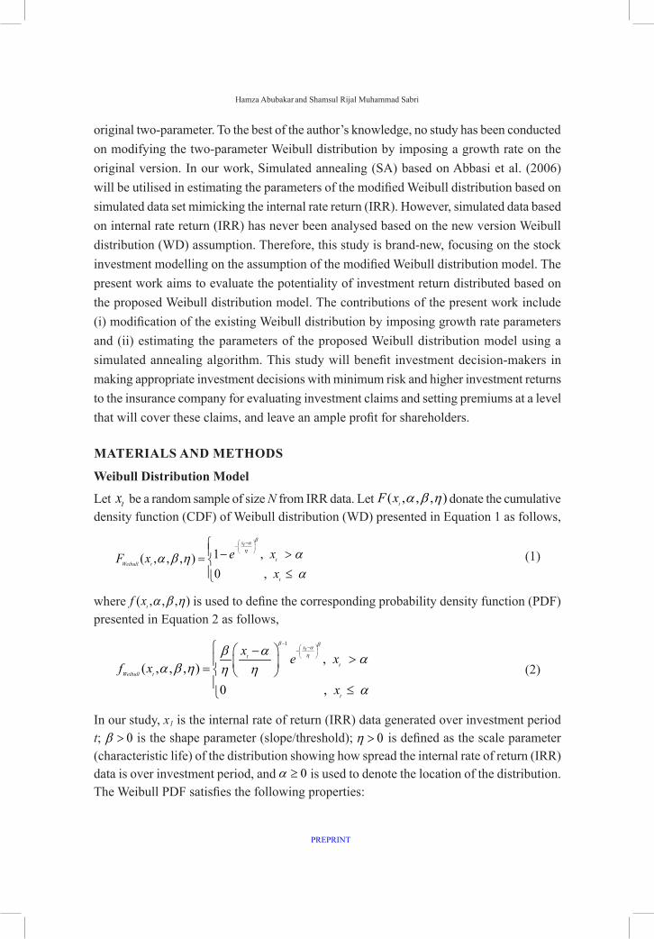
Let tx be a random sample of size N from IRR data. Let ( , , , )tF x α β η donate the cumulative density function (CDF) of Weibull distribution (WD) presented in Equation 1 as follows,

1 ,( , , , )0 ,

xt

tWeibull t

t

e xF xx

βαη αα β η

α

−−

− >= ≤

(1)

where ( , , , )tf x α β η is used to define the corresponding probability density function (PDF) presented in Equation 2 as follows,

1

,( , , , )

0 ,

xtt

t

Weibull t

t

x e xf x

x

β βαηαβ α

α β η η ηα

− −−

−> =

≤

(2)

In our study, x1 is the internal rate of return (IRR) data generated over investment period t; 0β > is the shape parameter (slope/threshold); 0η > is defined as the scale parameter (characteristic life) of the distribution showing how spread the internal rate of return (IRR) data is over investment period, and 0α ≥ is used to denote the location of the distribution. The Weibull PDF satisfies the following properties:


PREPRINT

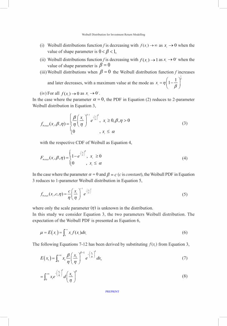
(i) Weibull distributions function f is decreasing with ( )tf x →∞ as 0tx +→ when the value of shape parameter is 0 1,β< <

(ii) Weibull distributions function f is decreasing with ( ) 1tf x → as 0tx +→ when the value of shape parameter is 0β =

(iii) Weibull distributions when 0β = the Weibull distribution function f increases

and later decreases, with a maximum value at the mode as 1

11txβ

ηβ

= −

(iv) For all ( ) 0tf x → as 0tx +→ .

In the case where the parameter 0α = , the PDF in Equation (2) reduces to 2-parameter Weibull distribution in Equation 3,

1

, 0, , 0( , , )

0 ,

xt

t

Weibull t

t

x e xf x

x

β β

ηβ β ηβ η η η

α

− −

≥ > =

≤

(3)

with the respective CDF of Weibull as Equation 4,

1 , 0( , , )0 ,

xt

tWeibull t

t

e xF xx

β

η

β ηα

−

− ≥= ≤

(4)

In the case where the parameter 0α = and cβ = (c is constant), the Weibull PDF in Equation 3 reduces to 1-parameter Weibull distribution in Equation 5,

1

( , , )c cxt

tWeibull t

xcf x c e ηηη η

− −

=

(5)

where only the scale parameter ( )η is unknown in the distribution.In this study we consider Equation 3, the two parameters Weibull distribution. The expectation of the Weibull PDF is presented as Equation 6,

( )0

( )t t t tE x x f x dxµ+∞

= = ∫ (6)

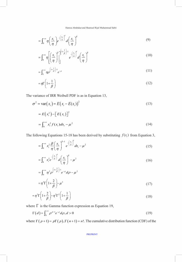
The following Equations 7-12 has been derived by substituting ( )tf x from Equation 3,

( )1

0

txt

t t txE x x e dx

ββηβ

η η

− − +∞

=

∫ (7)

0

txt

txx e d

β βη

η

− +∞

=

∫ (8)


PREPRINT

0

txt tx xe d

β βηη

η η

− +∞

=

∫ (9)

11 1

0

txt tx xe d

ββ ββηη

η η

+ − − +∞

=

∫ (10)

11 1

0eβ ρηρ

+ − +∞ − = ∫ (11)

11ηβ

= Γ +

(12)

The variance of IRR Weibull PDF is as in Equation 13,

( ) ( )22 var ( )t t tx E x E xσ = = − (13)

( ) ( ) 22t tE x E x= −

2 2

0( )t t tx f x dx µ

+∞= −∫ (14)

The following Equations 15-18 has been derived by substituting ( )tf x from Equation 3,1

2 2

0

txt

t txx e dx

ββηβ µ

η η

− − +∞

= −

∫ (15)

2 2

0

txt

txx e d

β βη µ

η

− +∞

= −

∫ (16)

21 12 2

0e dβ ρη ρ ρ µ

+ − +∞ − = −∫

2 221η µβ

= Γ + −

(17)

2 2 22 11 1η ηβ β

= Γ + − Γ +

(18)

where Γ is the Gamma function expression as Equation 19,

( ) 1

0, 0dd e d dρρ ρ

+∞ − −Γ = >∫ (19)

where ( ) ( ) ( )1 , 1 !p p p n nΓ + = Γ Γ + = . The cumulative distribution function (CDF) of the


PREPRINT

Weibull distribution can be obtained by integrating Equation 3 expressed as Equation 20,

( )0

( ) ( ) 1 exp tt t

xF x P x f d

ββ

ρ ρ ρη

= ≤ = = − −

∫ (20)

Weibull distribution interpolates between the standard exponential distribution when 1η = . It can be reduced to another special distribution called the Rayleigh distribution by setting the shape parameter 2β = . Several techniques have been used in estimating the unknown value of the Weibull distribution. In this study, a simulated annealing algorithm (SAA) incorporated in (MLE) has been utilised to maximise the Weibull distribution’s fitness function. To the best of the author’s knowledge, a simulated annealing algorithm (SAA) was not utilised to estimate the parameters of the modified version of Weibull distribution.

Mathematical Formulation of the Modified Internal Rate of Return Modelling

The investment strategy for holding the stock is allocating a level amount of contribution for K years at the beginning of the year. If we wish to hold the stock for the company chosen in the long term period, the stock valuation can also be seen by computing the (modified) internal rate of return (M)IRR). At the same time, if the company declares dividends yearly, the cash dividends are reinvested and together deposited with the level contribution to enlarging the share units. We let all our share units earn the share capital at the end of K years, indicating our investment profit. If our share capital is less than our total contribution, we may expect our MIRR to be in a negative form. The detailed procedure of the investment return was documented in Sabri and Sarsour (2019) is presented as Equations 21 and 22,

( ) ( )1,2

11,1 1,1 1,1 1,1(2)

11 1

365 365K

KK k

K u K K kk

u u u uNPV S P B r C rδ µ

+

++ +

=

− − = + + + − − + − ∑ (21)

( ) ( )1

1,1 1,1 1,1 1,1*

1( ) 1 1

365 365

KK k

kk

u u u uF K r C r

++ +

=

− −≡ + − − + −∑ (22)

where [ ]1,2,...,k K∈ is defined as the Net Present Value (NPV) of stock investment, computed at time zero. (2)

kS is accumulated share unit after share issuance at the end of the year k, which can be computed as Equation 23,

(2) (1)k k kS Sψ= × (23)

where kψ is the function of share issuance, k is the share units at the beginning of the year k, and F(K) is the terminal value investment fund to be let at the end of the year K K , which can be computed as Equation 24,

( 2)

1,2( ) K u K KK

F K S P B δ+

= × + + (24)


PREPRINT

where ,1ku represent the date of share purchased and sold, ,2ku , is the date of dividend and share issued based on the stock reported on year k,

,2kuP defined the stock price at the date ,2ku , kB represents the cash balance at the year k , Kδ defined as a cash dividend at year k, r represents the modified internal rate of return (MIRR) of the Malaysian property development companies (MPDS), C is the yearly fixed contribution which can be computed as Equation 25,

*

1k

k

CC

µ= (25)

It is very important to choose the best potential stocks to hold in the long term (long term investment). Furthermore, holding a stock for a K-years period of the investment may vary in terms of MIRR. For example, some might choose the best time to start investing, but it is tough to identify it as the MIRR measure can only be observed yearly. Therefore, assuming the MIRR for all starting times to invest is common, we may define the MIRR, denoted as tiKR , as a random variable having the mean and variance ( )KE R and ( )KVar Raccording to MIRR distribution.

Modified Internal Rate of Return on the assumption of Weibull Distribution

After acquiring the Weibull distribution parameters, a rate of return of the Malaysian property development sector (MPDS) can be observed for both short and long-term investment periods. In investment, we may obtain a positive value of profit (or even be greater than our capital investment) as well as poorly earn nothing. It indicates our capital of investment K could be infinite or even zero value. For some time K, our terminal investment ( )1 K

KC R+ is in between 0 to infinity Equation 26,

( )0 1 1K

tiK tiKC R R< + < ∞→ − < < ∞ (26)

since the rate of return is non-negative ( ). 1tiKi e R > − , we transformed the rate of return,

iKX τ according to Equation 27 as follows,

1iT iTX Rτ τ= + (27)

The Weibull distribution (WD) is flexible and easily applied in modelling many different forms of data (Thomas, 1995). The MIRR data will be modelled on the modified Weibull distribution (WD) assumption but the shape and scale parameters are unknown. The transformed MIRR data (X tiK) is assumed to come from the Weibull distribution (WD) in this study. A continuous random variable X tiK is said to follow Weibull distribution with parameters 0, 0K Kα β> > and 0Kη > to be estimated as follows ( ), ,tiK K K KX Weibull α β η�

if its PDF is given by Equation 28,


PREPRINT

1

,( , , , )

0 ,

KK XtiK K

tiK KK KtiK

X tiK K K KtiK K K

tiK

X e Xf X

X

ββ αηαβ αα β η η η

α

− − −

− > =

≤

(28)

From Equation (27), the mean of the three parameters WD is defined as Equation 29,

( ) 11tiK K K

K

E X η αβ

= Γ + +

(29)

where Γ signifies a gamma function of the parenthetic expression, defined as Equation 30,

1

0( ) x nn e x dx

∞− −Γ = ∫ (30)

The variance of the three parameters WD is a function of the shape ( )Kβ and scale parameters ( )Kη deduced as Equation 31,

( ) 2 22 11 1tiK

K K

Var X ηβ β

= Γ + −Γ +

` (31)

A higher variance would generally provide a lower investment return at the same point in time. If we wish to re-write the MIRR based on the Weibull distribution in Equation 28, we may have the following Equation 32,

( )( 1)1

( 1); , , , 1

KtiK KK

K

tiK

rtiK KK

r tiK K K K tiKK K

rf r e r

βαβ

ηαβα β ηη η

+ −− − + −

= > −

(32)

this will also indicate that mean and variance in Equations 29 and 31 can be re-written in terms of the transformed MIRR in Equations 33 and 34, respectively,

( ) 11tiK K K

K

E r η αβ

= Γ + +

(33)

( ) 2 22 11 1tiK K

K K

var r ηβ β

= Γ + −Γ +

(34)

Incorporating Growth Rate Parameter on Weibull distribution

The Internal rate of investment return (IRR) is usually used as a tool capable of evaluating


PREPRINT

the behaviour of cash flows (Sabri & Sarsour, 2019; Sarsour & Sabri, 2020a; Sarsour & Sabri, 2020b). Investigating the behaviour of investment return can be a challenging task due to its non-linearity, non-stationary, and high uncertainty. The Weibull distribution model is flexible in estimating components exhibiting increasing, constant and decreasing failure rate functions; however, it cannot directly fit those products with bathtub shapes or other non-monotonic failure rates functions such as internal rate of return and insurance claims data (Tang et al. 2002; Boonta & Boonthiem, 2019). The importance of such an extension has been proved in recent years on various problems. Many standard distributions have been generalised (Pobočíková et al., 2018). A list of well-being indicators may include profit, risk and uncertainly and failure rate (Boonta & Boonthiem, 2019). Those indicators also represent essential aspects of the investment return. In this context, it is necessary to modify the existing Weibull distribution that takes those characteristics into account. Parameters are added as viable alternatives to deal with the complexity and the multiple objectives that financial decisions can possess. The model considers the dynamic nature and uncertainty involved in the rate of return in taken investment decision which is assumed to undergo growth or decay according to some rate of investment return over the investment period (Kellison, 2009). We imposed a growth rate ( )ω for the investment period 2K ≥ that follows Equation 35,

( ) 1

11 K

tiK tiX Xω −

= + (35)

For 2 year investment period, the value 2,K = we have Equation 36,

( )2 11ti tiX Xω= + (36)

with the mean ( )tiKE X and the variance ( )tiKVar X in Equations 37 and 38, respectively as follows,

( ) ( ) ( )111 K

tiK tiE X E Xω −= + (37)

( ) ( ) ( )( )2111 K

tiK tiVar X Var Xω −= + (38)

Substituting Equations 35 and 36 into Equations 37 and 38, respectively yields Equations 39 and 40,

( ) ( ) 1 11 1KtiK K K

K

E X ω η αβ

− = + Γ + +

(39)

( ) ( )2

1 2 22 11 1 1KtiK K

K K

Var X ω ηβ β

− = + Γ + −Γ +

(40)


PREPRINT

For example, if 5K = , then the transformed MIRR of 5R based on Weibull distribution with PDF of three parameters will be Equation 41,

( )( )( )

( )( )

55 55

45

5

1115 55

545 5 5 5 5 5

1, 1; , , , 1

0

ti

ti

r

titiX ti

re rf X

Otherwise

βαβ

ω ηαβα β η ω η ω η

+ −− − +

+ − > −= +

(41)

According to Equation 32, the mean ( )tiKE X and the variance ( )tiKVar X of Equation 41 will be Equations 42 and 43,

( ) ( ) ( )45 51ti tiE X E Xω= + (42)

( ) ( )2

4 2 25

2 1var 1 1 1ti KK K

X ω ηβ β

= + Γ + −Γ +

(43)

By setting 0Kα = , Equation (41) is transformed into three-parameter Weibull distribution with ω a growth rate as Equation 44,

( ) ( )( )

5

5 54

5

5

115 5

545 5 5 5 5

, 0; , , 1

0

ti

ti

X

titiX ti

X e Xf X

Otherwise

ββ

ω ηββ η ω η ω η

− − +

>= +

(44)

If we consider the period of investment to be studied until K* years, for the sample size n and the maximum of the years that the data has been collected is T. We re-write Equation 44 in general form as Equation 45,

( ) ( )( ) 1

11

1 , 0; , , 1

0

K

K tiKK

K

tiK

X

tiKKtiKKX tiK K K K K

X e Xf X

Otherwise

ββ

ω ηββ η ω η ω η

−

− − +

−

>= +

(45)

For a period of investment, K, the ML of a random sample of 1 2 3 *, , ,..., Kx x x x size K*, where *K K∈ has been considered and the maximum investment period that MIRR data have been collected is T. The likelihood function of Weibull PDF in Equation 45 is presented as Equation 46,


PREPRINT

( )( )

( ) 1

1*

11

1 1

| , , 01

KK tiK

KK

tiK

Xn K

tiKKR tiK K K tiKK

i K K K

XL f X e X

ββ

ω ηββ η ωη ω η

−

− − +

−= =

= = >

+ ∏ ∏

(46)

The likelihood function of Weibull PDF in Equation 46 can be simplified to factor tiK KX and η and tiK KX and η as Equation 47,

( )( ) 1

1*

111

1

11

KK tiK

KKK

tiKK

XK

KK

K K

X e

ββ

ω ηββ

βη ω

−

− − +−

−=

=

+ ∏ (47)

The likelihood function of Weibull PDF is presented in Equation 47 can be simplified as Equation 48,

( )( )

( ) ( )( )

( )

( )( 1)*

1( 1) 1 1

1 1 1

1 1* *1*

11 1 1 1 1

1 1; 1X

n T KK nK n

tiK tiKT t i

T K T KK K nT KK tiK

KK t K t i

K tL X X eβ

η ωβ β

β

ξ βη ω − − − +− − − −

= = =

− − − −− −

−= = = = =

= =

∑ ∑ ∑ ∑ ∑∑ ∑ = × + × × ∏∏∏

(48)

The Log-likelihood function of Equation 48 is presented as Equation 49,

( ) ( ) ( ) ( )( )

( )( )

( )( )

( )

*

1

1 1* *

11 1 1 1 1 1

* * 1| * 1 ( ) ( ) 1 ( 1)

2

( 1) 1 11

K

tiKK

T K T KK n K ntiK

KtiKK t i K t i

K KInL X n K T In In n K T K

XIn Xβ

ξ β η β

β ω βη ω

=

− − − −

−= = = = = =

+ = − + − + − − − −

− + + − − +

∑

∑ ∑ ∑ ∑ ∑ ∑

(49)

where a vector ( ), ,K Kξ β η ω∈

is described as model parameters to be estimated. The vector ( )L ξ

is considered as a non-linear objective function and ξ

is taken as a decision

variable, the problem can be taken as an unrestricted nonlinear optimisation problem that could then be computed by maximising the Weibull distribution based on the simulated annealing (SAA) procedure proposed by Abbasi et al. (2006) presented in the next section.

( ) ( ) ( ) ( )( )

( )( )

( )( )

( )

*

1

1 1* *

11 1 1 1 1 1

* * 1| * 1 ( ) ( ) 1 ( 1)

2

( 1) 1 11

K

tiKK

T K T KK n K ntiK

KtiKK t i K t i

K TInL X n K T In In n K T K

XIn X

ξ β η β

β ω βη ω

=

− − − −

−= = = = = =

+ = − + − + − − − − − + + − − +

∑

∑ ∑ ∑ ∑ ∑ ∑

(50)

It is quite difficult and exhaustive to search the parameters of Equation 50 to attain the


PREPRINT

complicated objectives function as observed by Abbasi et al. (2006), Abbasi et al. (2011), and Yonar and Pehlivan (2020). Metaheuristics algorithms have been incorporated to reduce the complication involved in estimating the parameters,

Simulated Annealing Algorithm (SAA)

Simulated annealing (SAA) is one of the first single-based stochastic metaheuristics optimisation algorithms. It is inspired by the simulated thermodynamic process used in metallurgic for solidification studied in statistical mechanics, in which a material changes state while reducing its energy state to the lowest level (Kirkpatrick et al., 1983). Simulated annealing is considered one of the most powerful computation methods applied in solving the optimisation problem in almost every area. This physical process occurs after the metal is removed from the heat source. When the molten material is physically rinsed, the temperatures are decreased very slowly as heat passes to the surrounding environment to crystallise into one large crystalline lattice structure, and metal becomes solid at this stage. The energy has reached its minimum level. The SAA can be slow in reaching the optimal solution because optimal results require a very slow lowering of the temperature with control from iteration to iteration (well organised and perfect structure). The resulting lattice structure is probably not ideal if the crystallisation is too fast (imperfect structure). The advantages SAA possessed over other metaheuristics include; easy implementation, finding a globally optimal solution that is feasible even after finding a locally optimal solution, and satisfactory results are guaranteed with a relatively low number of iterations.

Generally, the SAA algorithm is based on the stochastic search technique, which generates perturbation of the current state at a random instance that make up the solution area which later undertakes series of operations such as initialisation, measure the quality of the solution, and if it is better than the new one, accept the solution that could lead a better searching technique of the SAA, to escape from local optima and to be in close vicinity of the region where the optimal solution could be located quickly. Since its implementation, SAA has been updated and extended to many mathematical and engineering domains. In this work, a robust and powerful heuristics search technique known as SAA has been established for effectively searching the MLE fitness function for Weibull Distribution based on simulated data set mimicking the internal rate of return. In this regard, the steps of the SAA implementation is presented in the next section.

SAA Implementation

A simulated annealing algorithm (SAA) is a two-step search process that includes perturbing the solution and evaluating its quality. Usually, to decide about the acceptance of the new solution, the algorithm uses the solution error. It is a stochastic method design to solve


PREPRINT

multidimensional global optimisation, i.e. problems with the following Equation 51,

( ) ( ) ( ) ( )min maxi i

opt optX Xf f or f f

ξ ξξ ξ ξ ξ

∈ ∈= =

(51)

where the variable i Xξ ∈ is variable to be estimated via SAA. This representation is common to most optimisation algorithms. However, SAA is a temperature-dependent search procedure and the process temperature. Let iτ be represented as the process temperature as Equation 52,

( )min max min1i T T Tτ λ τ λ λ= + ∗ − (52)

where min

Tλ and maxTλ are defined as the initial and final temperatures, N is the number of

temperatures, and the values of 1 [0, ]Nτ ∈ are chosen based on a specific cooling schedule considered problem-dependent. It is advisable to repeat a fixed number of iterations at each temperature before the temperature drops to enhance the performance of SAA.

There are some specific criteria to accept a solution once it has been perturbed. One obvious requirement is to accept a solution whenever there is less error than the previous solution. The metropolis algorithm has been used in SAA to compute the probability of acceptance for a perturbed solution. During the annealing process, each new solution ix was accepted with a temperature-dependent probability TP given by Equation 53,

( ) ( )( ) ( )

( ) ( ),

1

j i

T

j i

f x f xTk

j i

if f x f xP

e if f x f x≤

≤

= ≥

(53)

where T is the current temperature, and ( ) ( )i jf x and f x and ( ) ( )i jf x and f x are the fitness scores of the worst vertex ix and new vertex of the simplex, respectively.

Performance Evaluation

Several tests were carried out to examine the suitability of the proposed modified Weibull distribution in describing the behaviour of investment return in terms of the accuracy and error accumulations during the parameter estimation process. The performance of the proposed model has been evaluated in terms of their R-square(R2), mean absolute error (MAE), root means squared error (RMSE), Akaike’s information criterion (AIC), and the Kolmogorov-Smirnov test (KS) to ascertain the difference between the true and estimated distribution functions. The formulation of the statistical test used is presented in Equations 54-58, respectively,


PREPRINT

�( )�( ) �( )

2

2 12 2

1 1

( )

( ) ( ) ( )

n

tiKi

n n

tiK n tiK tiKi i

F X FR

F X F F X F X

=

= =

− = − + −

∑

∑ ∑ (54)

�( )2

1

1 ( )n

tiKi

RMSE F X Fn =

= − ∑ (55)

�

1

1 ( )n

tiKi

MAE F X Fn =

= −∑ (56)

( )2 2AIC k InL ξ= − (57)

� ( ) ( ) � ( )1 1

max maxtiK tiK tiK ii n i n

KS F X F X F X P≤ ≤ ≤ ≤

= − = − (58)

where � ( )tiKF X and F described the observed and the estimated parameters respectively, n defined as the total number.

Simulation Study

This section extends the two-parameters Weibull distribution to three Weibull distributions by imposing growth rate parameters on the existing Weibull model. The purpose is to investigate the long-term investment return that allows for identifying and forecasting company performance. Forecasting business return is necessary to properly analyse the business performance in either short-term or long-term periods. The analysis was conducted based on simulated data mimicking the internal rate of return (IRR). The parameters have been estimated for every sample size. We set the proposed Weibull distribution on the random variable X to mimic the simulation experiment’s internal rate returns (IRR). The samples of different sizes [10,100]n∈ were generated using Microsoft Excel 365. The parameters have been estimated via a programme executed on a Python programming language. Finally, the performance has been computed based on the goodness of fit using Microsoft Excel 365 for transparency.

Experimental Study

This section presents the experimental study used to analyse and compare the simulated data’s fitness on the proposed model. First, the experimental methodology applied in this study, the definition of the algorithm and parameters are presented. Then, the experimental results and the statistical tests carried out to evaluate these results are outlined. Finally, a

m a x m a x


PREPRINT

discussion based on the performance of the proposed methodology is provided. A dataset randomly generated were used in conducting the statistical analysis and evaluating the proposed Weibull model performance. The following procedures are adopted to generate random samples on the assumption of both the proposed and the existing models;

(i) choose starting values for the scale, shape, and growth rate parameters and determine the sample size n;

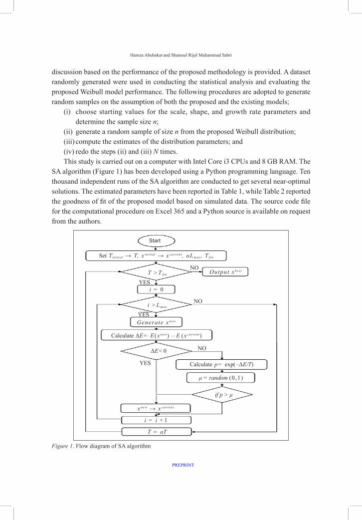
(ii) generate a random sample of size n from the proposed Weibull distribution;(iii) compute the estimates of the distribution parameters; and(iv) redo the steps (ii) and (iii) N times.This study is carried out on a computer with Intel Core i3 CPUs and 8 GB RAM. The

SA algorithm (Figure 1) has been developed using a Python programming language. Ten thousand independent runs of the SA algorithm are conducted to get several near-optimal solutions. The estimated parameters have been reported in Table 1, while Table 2 reported the goodness of fit of the proposed model based on simulated data. The source code file for the computational procedure on Excel 365 and a Python source is available on request from the authors.

Figure 1. Flow diagram of SA algorithm

Start

Set Tinit ial → T, x ini t ial → x current, αL max, T fin

T >T fin

i >L max

NO

NO

YES

Output x best

Generate x new

i = 0

YES

Calculate ΔE= E(x new) – E (x current)

YES

NO

Calculate p= exp(–ΔE/T)

ΔE<0

if p > μ

μ = random (0 ,1)

x new → x current

i = i +1

T = αT


PREPRINT

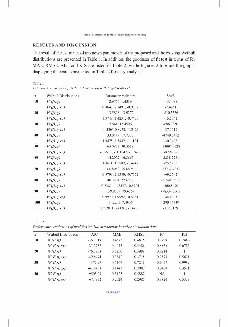
Table 2Performance evaluation of modified Weibull distribution based on simulation data

n Weibull Distribution AIC MAE RMSE R2 KS10 W(β,η) -36.0919 0.4375 0.4815 0.9799 0.7466

W(β,η,ω) -21.7737 0.4045 0.4486 0.8856 0.678520 W(β,η) -76.1838 0.5250 0.5989 0.3214 1

W(β,η,ω) -49.5474 0.3342 0.3718 0.9578 0.563130 W(β,η) -1377.97 0.5167 0.7248 0.7077 0.9999

W(β,η,ω) -61.0438 0.1443 0.2083 0.8400 0.351140 W(β,η) -9503.09 0.5125 0.5882 NA 1

W(β,η,ω) -67.4992 0.2624 0.2985 0.9820 0.5339

RESULTS AND DISCUSSION

The result of the estimates of unknown parameters of the proposed and the existing Weibull distributions are presented in Table 1. In addition, the goodness of fit test in terms of R2, MAE, RMSE, AIC, and K-S are listed in Table 2, while Figures 2 to 6 are the graphs displaying the results presented in Table 2 for easy analysis.

Table 1Estimated parameter of Weibull distribution with Log-likelihood

n Weibull Distributions Parameter estimates LogL 10 W(β,η) 2.9756, 1.4319 -13.7038

W(β,η,ω) 0.8647, 2.1491, -0.9832 -7.425120 W(β,η) 13.5808, 13.9272 -810.5536

W(β,η,ω) 1.3748, 1.4231, -0.7430 -15.534230 W(β,η) 7.644, 12.4506 -686.9850

W(β,η,ω) -0.5301,0.8923, -1.2423 -27.521940 W(β,η) 33.0149, 17.7373 -4749.5452

W(β,η,ω) 1.0475, 1.5442, -1.1191 -30.749650 W(β,η) 65.0825, 39.5618 -14997.9228

W(β,η,ω) -0.2513, -11.1642, -1.2499 -82.676560 W(β,η) 14.2972, 16.3663 -2238.2231

W(β,η,ω) 1.0611, 1.5789, -1.4742 -25.520170 W(β,η) 66.8042, 65.6898 -23732.7831

W(β,η,ω) 0.9798, 2.1389, -0.7372 -69.354280 W(β,η) 48.3294, 22.6938 -15548.6651

W(β,η,ω) 0.8383, 46.8547, -0.9204 -260.867090 W(β,η) 159.9159, 79.6757 -78334.6861

W(β,η,ω) 0.9979, 1.9992, -0.5261 -84.0295100 W(β,η) 11.2265, 7.4906 -2904.6339

W(β,η,ω) 0.92011, 2.6081, -1.4491 -112.6159


PREPRINT

Figure 2. MEA Evaluation of models performance

10 20 30 40 50 60 70 80 90 100SAMPLE SIZE

0.1

0.2

0.3

0.4

0.5

0.6

ME

AN

AB

SO

LU

TE

ER

RO

RS

Proposed method Existing method

Figure 3. RMSE Evaluation of models performance

Table 2 (continue)

n Weibull Distribution AIC MAE RMSE R2 KS50 W(β,η) -19010.2 0.51000 0.5860 N A 1

W(β,η,ω) -171.3530 0.2298 0.2838 0.8752 0.580260 W(β,η) -4480.45 0.5083 0.5845 NA 1

W(β,η,ω) -57.0402 0.2666 0.3100 0.9922 0.547270 W(β,η) -47469.6 0.5071 0.5835 NA 1

W(β,η,ω) -144.7083 0.2965 0.3508 0.9849 0.622280 W(β,η) -31101.3 0.5062 0.5828 NA 1

W(β,η,ω) -527.7340 0.4853 0.5590 0.9977 0.961590 W(β,η) -62206.7 0.5055 0.5822 NA 1

W(β,η,ω) -174.0589 0.2987 0.3451 0.9845 0.6076100 W(β,η) -124417 0.505 0.5082 0.5082 1

W(β,η,ω) -231.2317 0.3052 0.3618 0.9831 0.6631

10 20 30 40 50 60 70 80 90 100SAMPLE SIZE

0.2

0.4

0.6

0.8

RO

OT

ME

AN

SQ

UA

RE

ER

RO

RS


SAMPLE SIZE

MEA

N A

BSO

LUTE

ER

RO

RS

SAMPLE SIZE

RO

OT

MEA

N S

QU

ARE

ERR

OR

S


PREPRINT

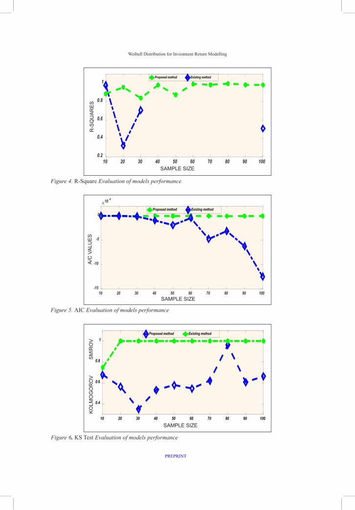
Figure 4. R-Square Evaluation of models performance

Figure 5. AIC Evaluation of models performance

Figure 6. KS Test Evaluation of models performance

10 20 30 40 50 60 70 80 90 100SAMPLE SIZE

0.2

0.4

0.6

0.8

1

R-S

QU

AR

ES


10 20 30 40 50 60 70 80 90 100SAMPLE SIZE

-15

-10

-5

0

AIC

VA

LU

ES

10 4


10 20 30 40 50 60 70 80 90 100SAMPLE SIZE

0.4

0.6

0.8

1

KO

LM

OG

OR

OV

–S

MIR

NO

V


SAMPLE SIZE

R-S

QU

ARES

SAMPLE SIZE

A/C

VAL

UES

SAMPLE SIZE

KOLM

OG

OR

OV

S

MIR

OV


PREPRINT

The estimated parameters and loglikelihood values of the proposed and the existing Weibull model have been reported in Table 1. It could be observed that all the estimated values showed a proper consistency based on the MAE and RMSE, which seem to decrease as the sample size increases in both models. Comparing the proposed model with the existing two parameters Weibull distribution, the results revealed that the proposed method produces the best-fit results in terms of MAE, RMSE, and R-square statistics in most of the cases. Therefore, according to the AIC value, the existing Weibull model is the better choice. The results in Table 2 have been displayed in Figures 1 to 5 for better analysis.

The results in Table 2 have been displayed in Figures 2-6 in evaluating the suitability of the proposed model in fitting the simulated data using MAE, RMSE, R-square, AIC, and KS test throughout the optimisation process. The best model was evaluated according to minimum MAE, RMSE, AIC, KS values, and high R-square values. Figures 2 and 3 displayed the MAE and RMSE of the simulated data from n = 10 to 100 sample size, mimicking IRR data on the assumption of the proposed model. It is observed that the error accumulation in the existing two-parameter Weibull distribution is constantly high with the increase in sample size for different values of the parameters. On the other hand, the errors decrease slightly with the increase in sample size. For example, at a sample of size 80, the MAE and RMSE increase but decrease as the sample size increases. In Figure 4, the R-square statistics have been displayed.

According to the R-square value of the Weibull models, the proposed model displayed high value through the simulation than the existing model. It is noticed that the existing Weibull model is found more complex in calculating the R-square value based on simulated data. It might be due to a large amount of error accumulation as the sample size increases. The R-square value cannot be computed when the sample size is high ( ). 20i e n > . R-square exceeds the threshold with the increase in sample size in the existing model. It reveals that the simulated data does not follow the model closely enough to make predictions confidently and that the data does not appear to follow a specific pattern. In Figure 4, Akaike’s information criterion (AIC) has been displayed based on Table 3. According to AIC values, the existing model is the better choice. The “best” model will be the one that neither under-fits nor over-fits. Although the AIC will choose the best model from a set of models, it will not say anything about the absolute quality of the model.

However, the existing model is still as good as the proposed one according to the AIC value. It shows that the existing model is nearly as good as the proposed model. The KS result in Table 2 has been displayed in Figure 5, showing the KS test of the proposed model as was less than that of the existing methods throughout the simulations experiments. The KS test of the existing Weibull distribution is 1 in some instances, especially as the


PREPRINT

sample size increases. It is an indication that the accumulation of the error is increasing as the sample size increases. It revealed that the CDF of the proposed model comes from the sample values that are equal to or less than x (i.e. sample data) (Dodge, 2008). Therefore, the proposed model is more accurate based on the simulated data used in this study. Consequently, the simulated data accepts the Weibull distribution at 95% confidence. The finding reveals that the existing two-parameter Weibull best fits a small sample size, while the accuracy of the proposed model increases as the sample size increases. The p-values are not that different for the smaller sample data. The proposed distribution model has the lowest values for all goodness-of-fit statistics among all fitted models. The analysis reveals that the proposed modified Weibull distribution provides a good fit to the simulated data sets by mimicking the internal rate of return (IRR).

CONCLUSION

A new distribution based on Weibull distributions has been proposed. Weibull distribution is used in modelling a wide variety of data, including wind speed, patient survival, and product lifetime. There has been an increasing interest in developing tractable lifetime models which fit financial data flexibly. This research proposed a new three-parameter Weibull distribution by imposing a growth rate parameter on the existing two parameters Weibull distribution model. Some of its characteristics include maximum likelihood function along with its characterisations. The estimation of the model parameters is obtained using the simulated annealing algorithm approach proposed by Abbasi et al. (2006). The experimental study was based on a simulated data set that mimicked the internal return rate for sample sizes 10 to 100. Based on the result presented in Tables 1 and 2, we presume that the proposed modified Weibull distribution will better fit IRR data when compared with the existing model. We have shown that the new modified Weibull distribution fits certain well-known data sets better than the existing Weibull distribution. Adding growth rate parameters by fixing one of the parameters still provides a better fit than existing models. Our future work is to extend the proposed model for the internal rate of return real-life data set. Statistical distributions such as gamma distribution, an exponentiated family of distribution, Pareto distribution and Rayleigh distribution can be modified to accommodate growth rate parameters to achieve better financial data fitting. Furthermore, the research will further explore various evolutionary computations and other metaheuristic algorithms to estimate the parameters of the proposed model.

ACKNOWLEDGEMENT

The authors would like to thank anonymous referees for their constructive comments on this manuscript. Special thanks to my humble supervisor for his helpful suggestions.


PREPRINT

REFERENCESAbbasi, B., Jahromi, A. H. E., Arkat, J., & Hosseinkouchack, M. (2006). Estimating the parameters of Weibull

distribution using a simulated annealing algorithm. Applied Mathematics and Computation, 183(1), 85-93. https://doi.org/10.1016/j.amc.2006.05.063

Abbasi, B., Niaki, S. T. A., Khalife, M. A., & Faize, Y. (2011). A hybrid variable neighborhood search and simulated annealing algorithm to estimate the three parameters of the Weibull distribution. Expert Systems with Applications, 38(1), 700-708. https://doi.org/10.1016/j.eswa.2010.07.022

Abubakar, H., & Danrimi, M. L. (2021). Hopfield type of artificial neural network via election algorithm as heuristic search method for random boolean ksatisfiability. International Journal of Computing and Digital System, 10(2), 660-673. http://dx.doi.org/10.12785/ijcds/100163

Abubakar, H., Rijal, S., Sabri, S. R. M., Masanawa, S. A., & Yusuf, S. (2020a). Modified election algorithm in hopfield neural network for optimal random k satisfiability representation. International Journal for Simulation and Multidisciplinary Design Optimization, 16(11), 1–13. https://doi.org/10.1051/smdo/2020008

Abubakar, H., M, S. A., Yusuf, S., & Abdurrahman, Y. (2020b). Discrete artificial dragonflies algorithm in agent based modelling for exact boolean k satisfiability problem. Journal of Advances in Mathematics and Computer Science, 35(4), 115-134. https://doi.org/10.9734/JAMCS/2020/v35i430275

Abubakari, A. G., Kandza-Tadi, C. C., & Moyo, E. (2021). Modified Beta Inverse Flexible Weibull Extension Distribution. Annals of Data Science, 1-29. https://doi.org/10.1007/s40745-021-00330-3

Almazah, M. M. A., Erbayram, T., Akdoğan, Y., AL Sobhi, M. M., & Afify, A. Z. (2021). A new extended geometric distribution: Properties, regression model, and actuarial applications. Mathematics, 9(12), 1336. https://doi.org/10.3390/math9121336

Almetwally, E. M. (2021). Extended odd weibull inverse rayleigh distribution with application on carbon fibres. Mathematical Sciences Letters, 10(1), 5-14. https://doi.org/10.18576/msl/100102

Alrashidi, M., Rahman, S., & Pipattanasomporn, M. (2020). Metaheuristic optimization algorithms to estimate statistical distribution parameters for characterizing wind speeds. Renewable Energy, 149, 664-681. https://doi.org/10.1016/j.renene.2019.12.048

Alzaatreh, A., Lee, C., & Famoye, F. (2013). A new method for generating families of continuous distributions. Metron, 71(1), 63-79. https://doi.org/10.1007/s40300-013-0007-y

Alzaeemi, S. A., & Sathasivam, S. (2020). Artificial immune system in doing 2-satisfiability based reverse analysis method via a radial basis function neural network. Processes, 8(10), Article 1295. https://doi.org/10.3390/pr8101295Bidrama, H., Behboodian, J., & Towhidib, M. (2013). The beta weibull-geometric distribution. Journal of Statistical Computation and Simulation, 83(1), 52-67. https://doi.org/10.1080/00949655.2011.603089

Boonta, S., & Boonthiem, S. (2019). An approximation of minimum initial capital of investment discrete time surplus process with Weibull distribution in a reinsurance company. Journal of Applied Mathematics, 2019, Article 2191509. https://doi.org/10.1155/2019/2191509

Chauhan, S. K., & Malik, S. C. (2017). Evaluation of reliability and MTSF of a parallel system with Weibull failure laws. Journal of Reliability and Statistical Studies, 10(1), 137-148.


PREPRINT

Datsiou, K. C., & Overend, M. (2018). Weibull parameter estimation and goodness-of-fit for glass strength data. Structural Safety, 73, 29-41. https://doi.org/10.1016/j.strusafe.2018.02.002

Freitas de Andrade, C., dos Santos, L. F., Macedo, M. V. S., Rocha, P. A. C., & Gomes, F. F. (2019). Four heuristic optimization algorithms applied to wind energy: Determination of Weibull curve parameters for three Brazilian sites. International Journal of Energy and Environmental Engineering, 10, 1-12. https://doi.org/10.1007/s40095-018-0285-5

Dodge, Y. (2008). Kolmogorov–Smirnov test. In The concise encyclopedia of statistics (pp. 283-287). Springer. https://doi.org/10.1007/978-0-387-32833-1_214

Elmahdy, E. E., & Aboutahoun, A. W. (2013). A new approach for parameter estimation of finite Weibull mixture distributions for reliability modeling. Applied Mathematical Modelling, 37(4), 1800-1810. http://doi.org/10.1016/j.apm.2012.04.023

Guedes, K. S., de Andrade, C. F., Rocha, P. A., Mangueira, R. D. S., & de Moura, E. P. (2020). Performance analysis of metaheuristic optimization algorithms in estimating the parameters of several wind speed distributions. Applied Energy, 268, Article 114952. https://doi.org/10.1016/j.apenergy.2020.114952

Guerra, R. R., Peña-Ramírez, F. A., & Bourguignon, M. (2020). The unit extended Weibull families of distributions and its applications. Journal of Applied Statistics, 1-19. https://doi.org/10.1080/02664763.2020.1796936

Hashmi, S., Ahsan, M., Haq, U., Muhammad, R., & Ozel, G. (2019). The Weibull-Moment Exponential Distribution: Properties, Characterizations & applications. Journal of Reliability and Statistical Studies, 12(1), 1-22.

Hirose, H. (2002). Maximum likelihood parameter estimation in the extended Weibull distribution and its applications to breakdown voltage estimation. IEEE Transactions on Dielectrics and Electrical Insulation, 9(4), 524–536. https://doi.org/10.1109/TDEI.2002.1024429

Kaba, A., & Suzer, A. E. (2021). Metaheuristic data fitting methods to estimate Weibull parameters for wind speed data: A case study of Hasan Polatkan Airport. The Aeronautical Journal, 125(1287), 916-948. https://doi.org/10.1017/aer.2020.136

Kellison, S. G. (2009). The theory of interest (3rd Ed.). McGraw-Hill Education.

Kirkpatrick, S., Gelatt, C. D., & Vecchi, M. P. (1983). Optimization by simulated annealing. Science, 220(4598), 671-680. https://doi.org/10.1126/science.220.4598.671

Lee, C., Famoye, F., & Alzaatreh, A. Y. (2013). Methods for generating families of univariate continuous distributions in the recent decades. Wiley Interdisciplinary Reviews: Computational Statistics, 5(3), 219-238. https://doi.org/10.1002/wics.1255

Liao, Q., Ahmad, Z., Mahmoudi, E., & Hamedani, G. G. (2020). A new flexible bathtub-shaped modification of the Weibull model: Properties and applications. Mathematical Problems in Engineering, 2020, Article 3206257. https://doi.org/10.1155/2020/3206257

Okafor, E. G., Ezugwu, O. E., Jemitola, P. O., Sun, Y., & Lu, Z. (2018). Weibull parameter estimation using particle swarm optimization algorithm. International Journal of Engineering and Technology (UAE), 7(3), 7-10. https://doi.org/10.14419/ijet.v7i3.32.18380


PREPRINT

Okasha, H. M., & Basheer, A. M. (2020). On marshall-olkin extended inverse weibull distribution: Properties and estimation using type-II censoring data. Journal of Statistics Applications & Probability Letters, 7(1), 9-21. https://doi.org/10.18576/jsapl/070102

Phani, K.K. (1987). A New Modified Weibull Distribution. Communications of the American Ceramic Society, 184(August), 182-184. https://doi.org/10.1111/j.1151-2916.1987.tb05719.x

Pobočíková, I., Sedliačková, Z., & Michalková, M. (2018). Transmuted Weibull distribution and its applications. MATEC Web of Conferences, 157, 1-11. https://doi.org/10.1051/matecconf/201815708007

Sabri, S. R. M., & Sarsour, W. M. (2019). Modelling on stock investment valuation for long-term strategy. Journal of Investment and Management, 8(3), 60-66. https://doi.org/10.11648/j.jim.20190803.11

Sarhan, A. M., & Zaindin, M. (2009). Modified Weibull distribution. Applied Sciences, 11(January 2000), 123-136. https://doi.org/10.1051/matecconf/201815708007

Sarsour, W. M., & Sabri, S. R. M. (2020a). Evaluating the investment in the Malaysian construction sector in the long-run using the modified internal rate of return: A Markov chain approach. The Journal of Asian Finance, Economics, and Business, 7(8), 281–287. https://doi.org/10.13106/jafeb.2020.vol7.no8.281

Sarsour, W. M., & Sabri, S. R. M. (2020b). Forecasting the long-run behavior of the stock price of some selected companies in the Malaysian construction sector: A Markov chain approach. International Journal of Mathematical, Engineering and Management Sciences, 5(2), 296-308. https://doi.org/10.33889/IJMEMS.2020.5.2.024

Sathasivam, S., Mansor, M., Kasihmuddin, M. S. M., & Abubakar, H. (2020). Election algorithm for random k satisfiability in the Hopfield neural network. Processes, 8(5), Article 568. https://doi.org/10.3390/pr8050568

Tang, Y., Xie, M., Lai, C. D., & Goh, T. N. (2002). Statistical analysis of a Weibull extension model, communications in statistics. Theory and Methods, 32(5), 913-928. https://doi.org/10.1081/STA-120019952

Thomas, G. M. (1995). Weibull parameter estimation using genetic algorithms and a heuristic approach to cut-set analysis (Doctoral dissertation). Ohio University, USA.

Wang, M., & Elbatal, I. (2015). The modified Weibull geometric distribution. Metron, 73(3), 303-315. https://doi.org/10.1007/s40300-014-0052-1

Yonar, A., & Pehlivan, N. Y. (2020). Artificial bee colony with levy flights for parameter estimation of 3-p Weibull distribution. Iranian Journal of Science and Technology, Transactions: Science, 44, 851-864. https://doi.org/10.1007/s40995-020-00886-4

a simulation study on modified weibull distribution for

Documents