a simulation-based serious game in appointment scheduling

A SIMULATION-BASED SERIOUS GAME IN APPOINTMENT

SCHEDULING FOR SERVICE FACILITIES IN HEALTHCARE

Bachelor Thesis Industrial Engineering and Management

8 SEPTEMBER 2021 UNIVERSITY OF TWENTE

Sander van den Berg ADVISORY COMMITTEE:

First supervisor: prof.dr.ir. E. Hans External supervisor Rhythm: ir. R. Vromans

1

Management summary Background

This thesis presents a simulation-based serious game in healthcare. This thesis is

motivated from the observation that stakeholders have little intuition about logistic

processes behind their services. Stakeholder are mostly healthcare professionals in

training. The logistic process that is concerned is appointment scheduling in healthcare

with multiple types of arrivals.

Objective

Stakeholders are educated through active learning by the use of a simulation-based

serious game. The user can manipulate input parameters on a dashboard and see the

influence of their decisions in output parameters. The goal is to understand the relation

between a defined set of input parameters and the output parameters. Additionally,

the user is guided during the game.

Approach

The design of the simulation-based serious game is supported by two methodologies.

One methodology concerns the overall structure from development to

experimentation. The other methodology concerns the conceptualization. The

simulation-based serious game is developed in the R language environment.

The simulation primarily concerns the process of appointment scheduling with three

types of (optional) arrivals: scheduled, unscheduled and emergency patients. The

main outputs are the average waiting and access time. Other input and output

parameters concern no-show probability, balking patients, reneging patients, service

times and utilization/idleness.

Conclusion

The simulation has a value for practice as the simulation-based serious game is

verified, validated and is successfully able to replicate a realistic hospital environment.

The simulation-based serious game is a contribution to the field of serious games and

science as there are only little existing serious games in appointment scheduling. This

contribution is a value for science.

To create a hospital environment the user can alter input parameters and observe

output parameters in a dashboard accessible through the webserver. This active

learning process enables the user to create more intuition in appointment scheduling.

Further work

The simulation-based serious game is still to be put to practice to professional and

experienced user in the field of healthcare. This allows to effectively evaluate the

simulation based serious-game. Also, other operation management concepts in

healthcare (i.e. pooling effect, integral capacity management) can be illustrated in a

similar serious game.

2

Foreword The thesis in front of you concludes my bachelor assignment for the study Industrial

Engineering and Management at the University of Twente. In contrast to many other

theses, our research is not executed at an external organization because of the COVID-

lockdown situation. Hence my thesis tackles an irregular problem. Nevertheless there

is an external problem owner at hand who has a strong interest in the outcome of the

research.

In contribution to the work we provided, I would like to thank the advisory committee

for their support in the establishment of the Thesis. First and foremost I would like to

thank prof.dr.ir. Erwin Hans, who was able to consistently inspire me with his

inexhaustible positivism. He was always available for any type of concerns, he

consistently helped me in the right direction of the thesis by delivering useful feedback

that I could process into content. Also because of him, I was able to significantly

improve my academic writing style. Second, I would like to thank Rob Vromans from

Rhythm B.V. Rob is a consultant in healthcare and was able to transmit his knowledge

and expertise into feedback necessary for the development of the tool. I could not have

(started and) finished my thesis without them.

Finally, I would like to thank many others for their support in my personal and social

circumstances. I would like to thank my roommates, my girlfriend, my family, and

friends for their support in successfully fulfilling my bachelor thesis. Additionally, I

would thank C. ten Napel for his constructive support during all of my bachelor years.

Sander Constantijn Bijn van den Berg

Enschede, September 2021.

3

Table of Contents Management summary ........................................................................................................... 1

Background ........................................................................................................................... 1

Objective ................................................................................................................................ 1

Approach .............................................................................................................................. 1

Conclusion ............................................................................................................................ 1

Further work ......................................................................................................................... 1

Foreword .................................................................................................................................. 2

Glossary of terms ..................................................................................................................... 5

Chapter 1 – Introduction ........................................................................................................ 6

1.1 Motivation of the Research ...................................................................................... 6

1.2 Problem description ................................................................................................. 7

1.3 Objective and approach ................................................................................................ 7

Chapter 2 – Systematic approaches for designing a serious game .................................. 8

2.1 Introduction to serious games ..................................................................................... 8

2.2 Taxonomy of serious games ......................................................................................... 9

2.3 Methodologies .............................................................................................................. 10

2.3.1 Game design. ............................................................................................................. 10

2.3.2 Conceptual framework for simulation-based serious games ............................. 10

Chapter 3 – Application of the conceptual framework for simulation-based serious

games ....................................................................................................................................... 11

3.1 Step 1: Understanding the learning environment ................................................... 11

3.1.1 Mixed appointment scheduling in healthcare .................................................. 11

3.1.2 Discrete-event Simulation .................................................................................... 12

3.1.3 Appropriate game format .................................................................................... 12

3.2 Step 2: Determine objectives ...................................................................................... 12

3.2.1 Pedagogic purpose ................................................................................................ 12

3.2.2 Modeling objectives .............................................................................................. 13

3.2.3 General project objectives .................................................................................... 13

3.3 Step 3: Model outputs ................................................................................................. 13

3.4 Step 4: Model inputs .................................................................................................... 14

3.5 Step 5: Model content .................................................................................................. 14

3.6 Mock-up ........................................................................................................................ 15

Chapter 4 – Construction and modification ...................................................................... 16

4

4.1 Toolbox .......................................................................................................................... 16

R ........................................................................................................................................ 16

Rshiny .............................................................................................................................. 16

4.2 Model development .................................................................................................... 16

4.2.1 Simulation model .................................................................................................. 16

4.2.2 Verification of Parameters ................................................................................... 18

4.3 User Interface ............................................................................................................... 20

4.4 Verification of the Conceptualization ....................................................................... 21

Chapter 5 – Accessibility and validation ........................................................................... 22

5.1 Accessibility .................................................................................................................. 22

5.2 Validation of the model .............................................................................................. 22

5.2.1 Validation of the input parameters .................................................................... 22

5.2.2 Validation of outputs ............................................................................................ 28

5.3 Limitations and assumption of the model ............................................................... 29

5.3.1 Limitations ............................................................................................................. 29

5.3.2 Assumptions: ......................................................................................................... 30

Chapter 6 - Experimentation ................................................................................................ 31

Experimentation ................................................................................................................. 31

Experiment 1: Facility X ................................................................................................ 31

Experiment 2: CT-Scan AMC ....................................................................................... 33

Learning context ................................................................................................................ 35

Chapter 7 - Conclusion & discussion ................................................................................. 36

References ............................................................................................................................... 38

Appendices ............................................................................................................................. 40

Appendix 1: Criteria of the taxonomy ........................................................................ 40

Appendix 2: Outline of the conceptual framework for simulation-based gaming

........................................................................................................................................... 40

Appendix 3: URLs to tools and codes ......................................................................... 42

Appendix 4: Screenshots of UI ..................................................................................... 43

Appendix 5: Operator’s Manual .................................................................................. 44

Additional figures .............................................................................................................. 47

5

Glossary of terms Terms:

Access time The time between the appointment request and appointment time

Waiting time

The time between the arrival at the facility and the start of the activity.

Preemption The act of claiming a resource above others, even if it is in process.

Renege To fall back on a prior state or abandoning the system.

Balk Impossibility to seize a resource and thus leaving.

Abbreviations:

SAR Scheduled Arrival(s) (Rate(s)) / Scheduled patients

UAR Unscheduled Arrival(s) (Rate(s)) / Unscheduled patients

EAR Emergency Arrival(s) (rate(s))/ Emergency patients

OM Operations Management

DES Discrete-event Simulation

6

Chapter 1 – Introduction In this introductory chapter we outline the research motivation and research plan.

Section 1.1 gives a motivation of the research and introduces the problem, section 1.2

describes the problem and section 1.3. elaborates on the objective and approach for this

research.

1.1 Motivation of the Research

No industry can survive without recognizing the importance of reducing costs

wherever it may be possible, the healthcare sector is no exception. It is observed that

inefficiencies in logistics are one of the most significant cost drivers. Optimizing the

logistics within healthcare institutions reduce theses costs and additionally influence

patients satisfaction and decrease serious health risks. Therefore, it is important to

provide a better quality of service.

Figure 1 depicts the problem cluster we have at hand. We can assess that there are

multiple causes influencing the performance (utilization of doctors, waiting time, etc.)

of a healthcare institution. For the purpose and scope of this research, only a small

selection of problems is highlighted. The most important core problem is that

healthcare professionals often have a strong background in medical education but only

rudimentary training in OM. This little intuition that exists is regarded as one of the

reasons why there is a lack of implementation of already existing and proven solutions.

In anticipation of this, we introduce a simulation-based serious game that strives to

educate the concept of appointment scheduling. The use of serious games is chosen as

they encourage learners to learn by doing. It permits the learners to make decisions,

control their own moves, and interpret its influence on their own or by guidance. The

game is meant for a wider range of stakeholders than just healthcare workers.

The concept that we illustrate is inspired by the article “Designing Cyclic Appointment

Scheduled for Outpatient Clinics with Scheduled and Unscheduled Patient Arrivals”

by N. Kortbeek (Kortbeek et al., 2014). This paper developed an appointment schedule

for service facilities that process both scheduled and unscheduled arrivals. Serving

patients with multiple type of arrivals is found challenging as its consequences and

relation between parameters are hard to outweigh.

Figure I Problem cluster

7

1.2 Problem description

Most healthcare institutions only provide the possibility to schedule appointments in

advance on appointment slots, as there are multiple organizational and medical

reasons to give a patient an appointment. However, most institutions do not offer any

service on walk-in basis. To help decision-makers in the visualization of a walk-in and

appointment (mixed) system we design a simulation that incorporates an appointment

schedule system with the possibility to allow multiple types of arrivals: Scheduled

(SAR), Unscheduled (UAR) and Emergency (EAR) patients.

Advantages of allowing UAR and EAR arrivals in the system are a higher level of

accessibility, more freedom for a patient to choose a date and time for their visit and

(potential compensation of utilization loss. Disadvantages are a fluctuating variable

demand, which results in a higher waiting time for all patients, and potentially

neglecting UAR (or EAR).

The advantage of an appointment system (SAR) is that workload can be efficiently

dispersed, while the disadvantage is a longer access time.

Long access times can result in serious health risks due to a delay in treatment.

Allowing UAR & EAR into the system reduces the access time to zero, but increases

waiting time. Also, UAR & EAR can compensate utilization loss from SAR that do not

show up (no-show). The challenge within our game is thus to understand and cope

with a healthy balance between the access and waiting time.

1.3 Objective and approach

We aim to design a simulation that simulates a realistic environment. In this safe

environment the user can freely manipulate input and output parameters to have a

better understanding of appointment scheduling in healthcare, as the objective is to

ultimately create more intuition.

The thesis follows two methodologies that concern game design: the game design

methodology and the conceptual framework for simulation-based serious games. The

application is developed in R.

The outline of this thesis is organized as follows. Chapter 2 discusses systematic

approaches for serious games. In Chapter 3, we conceptualize our serious game.

Chapter 4-5 concerns the construction and modification of the game in terms of

development and implementation. Chapter 6 provides experimentation and puts the

serious game into practice. In chapter 7 we end with a conclusion and discussion.

8

Chapter 2 – Systematic approaches for designing a serious game This chapter elaborates on the systematic approaches for simulation-based serious

games and serious games in general. We start with an introduction to serious game

and its definitions. We continue with taxonomy on serious games. We end with an

elaboration on the methodologies used.

2.1 Introduction to serious games

The origin of games date to the ancient past and is considered an integral part of all

societies. Playing dice appears to be the oldest known example, which set his marks a

3000-year-old game set in south Iran (Laamarti et al., 2014). After which many

adaptations within the definition of gaming were developed. The general definition of

a game is defined as a physical and/or mental contest that is played according to

specific rules, with the sole goal of amusing or entertaining the participant(s). A video

game is a special type of game where the game is played with a computer according

to certain rules with the goal of amusement, recreation, or winning a stake (Laamarti

et al., 2014). Serious games are a combination of both and we distinguish serious games

into their own category.

The distinguishment can be found in the most common definition of serious games:

“games that do not have entertainment, enjoyment, or fun as their primary purpose”

(Laamarti et al., 2014). This does not mean that entertainment is excluded from serious

games. Definitions in literature encountered either in research or industry agree that

serious games include entertainment dimension (Jantke, 2010; Quinn & Neal, 2008;

Zyda, 2005). So does Lamaarti, as he defines a serious game as a game that combines

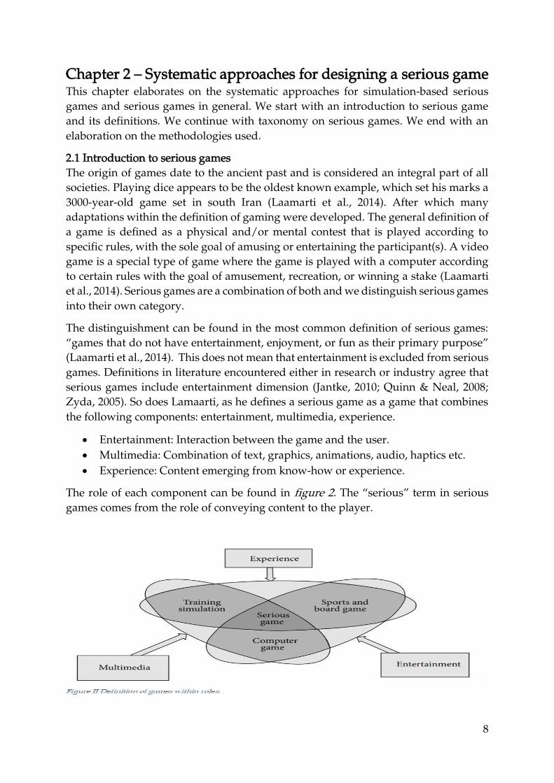
the following components: entertainment, multimedia, experience.

• Entertainment: Interaction between the game and the user.

• Multimedia: Combination of text, graphics, animations, audio, haptics etc.

• Experience: Content emerging from know-how or experience.

The role of each component can be found in figure 2. The “serious” term in serious

games comes from the role of conveying content to the player.

9

As the components that define the serious game are vast, it is important to classify its

existence into a specific domain. In the next section, we discuss the taxonomy of

serious games.

2.2 Taxonomy of serious games

The popularity and importance of serious games have only recently been recognized,

therefore only little research on their classification exists(News, 2015). Though there

are articles that attempt to categorize serious games, they merely explain the features

that are crucial in their design (Lope & Medina-Medina, 2017; Riedel & Hauge, 2011).

We conclude that a general taxonomy within serious games does most likely not exist.

Therefore, we fall back on the overview of a taxonomy discussed by Lamaarti.

Lamaarti defines a taxonomy within serious games that can be assessed by the game’s

characteristics. The criteria of these characteristics have the potential to make a

significant difference in the success of a serious game. The criteria that can be derived

are activity, modality, interaction style, environment, and application area. Figure 3

depicts the taxonomy of Lamaarti and in appendix 1 we summarize this taxonomy.

The taxonomy predicts that our game is most likely a simulation-based serious game.

Examples are Monte-Carlo simulations and Discrete-event Simulations. We reflect on

our game’s taxonomy in section 3.7.

Figure III Taxonomy of serious games

In the next section, we discuss the methodologies used in this thesis.

10

2.3 Methodologies

Our thesis combines two methodologies. “The Game Design” methodology and “The

Conceptual framework for simulation-based serious games”. The structure of the

report is based on these methodologies. The game design accounts the overall

structure and is supported in stage 1 by the methodology steps on the conceptual

framework of simulation-based serious games.

Overview of the approach:

1. Stage 1: Conceptualization

Step 1.1: Understanding the learning environment

Step 1.2: Determine objectives

Step 1.3: Identify the model outputs

Step 1.4: Identify the model inputs

Step 1.5: Determine the model content

2. Stage 2: Construction

3. Stage 3: Modification

4. Stage 4: Experimentation

5. Stage 5: Preparation for use by others

2.3.1 Game design.

The game design is a methodology designed by (Greenblat & Duke, 1981). This

methodology is summarized in figure 4. Greenblat distinguishes five stages in his

game design. The first three aim to address the objectives, model, and representation

of the game. While the latter two are meant to evaluate the use of the game. These steps

are useful in the development of the model by specifying the possibilities for model

pruning.

In the game design methodology “construction & modification” account for the

development and implementation phase, while the latter two account the

experimentation and evaluation phase. The first two stages address game construction

and include a preparatory task for game use. Apart from this methodology a

conceptual framework for simulation-based gaming is used. We follow a conceptual

framework as the concept is one of the most important elements in design writing.

Allowing a structural conceptualization provides guidance to the game designer.

2.3.2 Conceptual framework for simulation-based serious games

The conceptual framework for simulation-based gaming proposed by (Van Der Zee et

al., 2012) extends the Robinson framework (Robinson, 2008). The conceptual modeling

framework for simulation-based serious gaming distinguishes five key modeling

activities as can be seen in figure 5. These activities shape the headers of our sections

in the next chapter. In appendix 2 we outline this conceptual framework by van der

Zee.

11

Chapter 3 – Application of the conceptual framework for

simulation-based serious games This chapter applies the conceptual framework for the simulation based serious

games. The sections are divided according to the steps presented in the is conceptual

framework discussed in section 2.3.

3.1 Step 1: Understanding the learning environment

To understand the learning environment we perform literature research in the

following subject matters: Mixed appointment scheduling and Discrete-Event

Simulations. We end the section by determining the appropriate gaming format.

3.1.1 Mixed appointment scheduling in healthcare

As we all experience, many service facilities request customers to make an

appointment. Healthcare is considered to be the most prevalent application area of

appointment systems (Cayirli & Veral, 2009; Gupta & Denton, 2008). Therefore, we

speak of patients instead of customers. An appointment schedule involves (i) making

an appointment, (ii) accessing the appointment, (iii) waiting for, and (iv) performing

the activity of the appointment. These stages can be regarded as a combination of two

distinct queuing systems. The first queue concerns the patient to make an appointment

and wait until the particular slot (access process and concerning SAR only) and the

second concerns the process of the service once arrived at the institution (waiting and

activity process, concerning all types of patients). Queuing notations are noted as

A/B/c/N/K queues. The A represents the inter-arrival time distribution and the B

represents the service time distribution. The c represents the number of parallel servers

(s in Kendall’s notation). The N represents the system capacity. The K represents the

size of the calling population. Common symbols for A and B are M (exponential or

Markov), D (constant or deterministic), and G (arbitrary or general). Queues mostly

respect the FCFS principle (with possible prioritization). Literature shows that most

queueing systems in healthcare follow the M/M/s principle (Zonderland & Boucherie,

2012).

Most appointment scheduling systems for day appointment schedules have the same

typical objectives: minimizing patient waiting and access time, maximizing resource

(personnel and activity) utilization, minimizing resource idle time. (Kortbeek et al.,

2014). Also, the performance of these schedules is impacted by service and arrival

punctuality (e.g. deviations in activities, arrival rates, and no-shows, and other patient

behavior). Reasons for this punctuality can be that distinct priority levels translate into

patient type differentiation/

A mixed system considers patient tape differentiation. In studies (Borgman et al., 2018;

Holleman et al., 1996; Kortbeek et al., 2014; Sickinger & Kolisch, 2009) differentiation

is mostly made in Scheduled (SAR), Unscheduled (UAR), and Emergency (EAR)

patients. Scheduled patients have the probability to no show up, which leads to

utilization loss. Patients without an appointment are either Emergency patients who

have non-preemptive priority and Unscheduled patients who can walk in freely

12

during the day. Also, queues can generate balking and reneging behavior for

Unscheduled patients, meaning that unscheduled people leave or will not join the

queue if the queue is or takes too long (Shin & Choo, 2009).

3.1.2 Discrete-event Simulation

Different types of simulation can be applied depending on the nature of the system

under consideration. Our purpose is to simulate a real-world system that visualizes

the appointment scheduling process. Discrete-event simulation (DES) enables us to do

so. DES is a technique for modeling stochastic, dynamic, and discretely evolving

systems. There are many examples: Customers arriving at a bank, products being

manipulated in a supply chain, or patients wanting to make an appointment. The

discrete nature of a given system arises as soon as its behavior can be described in

terms of events, which is the most fundamental concept in DES. An event is an

instantaneous occurrence that may change the state of the system, while, between

events, all the state variables remain constant (Günal & Pidd, 2010; Zhang, 2018).

The discrete-event simulation in our case would be to model a certain queue, such as

patients arriving at a facility to be served by a CT-scan. In this example, the system

entities are patient queue (waiting list and waiting room) and CT-Scan. The system

events are patient-arrival and patient-Departure. The system states, which are changed

by these events, are the number of patients in the waiting list or room and CT-scan

status (busy or idle). The random variables that need to be characterized to model this

system are the patient inter-arrival times and CT-scan service times.

3.1.3 Appropriate game format

Game formats take the form of a board game, computer-based game etc. (Laamarti et

al., 2014). In this case, we decide that a computer-based gaming format is appropriate.

This computer-based gaming format runs a simulation in the background that can be

manipulated in the input parameters. These input parameters are synchronized with

according output parameters. The objective is to balance the input parameters to their

best extent. Consequently, the outputs can be observed and evaluated. Because this

system seems subjective, we aim to apply some sort of objective score that determines

the appropriateness of the choices made by the user. Also, the simulation can be

operated by an experienced person (operator, teacher, etc.) who can use the simulation

to support teaching.

3.2 Step 2: Determine objectives

As the framework proposes, we start by identifying the pedagogic purposes, the

modeling objectives, and general project objectives.

3.2.1 Pedagogic purpose

The pedagogic purpose concerns what the player should learn after playing the game.

The main objective is to develop more intuition about a mixed appointment schedule

system. We want the player to realize the potential of this mixed appointment system

in healthcare. As traditional appointment systems are currently regarded as the

13

popular (and in some cases the only) option, we emphasize on its contrast as we

compare it to a mixed system.

3.2.2 Modeling objectives

The player should anticipate by deciding on the implementation and manipulation of

the input parameters. As discussed in the subject matter three objectives are important.

(i) minimizing patient waiting and access time, (ii) maximizing resource utilization,

(iii) minimizing resource idle time. The use of these KPIs will be discussed in section

3.3. These KPIs are influenced by the access and waiting process.

The objective of the serious game is to simulate a hospital by choosing your own input

parameters. Afterward, the user can decide what kind of influence the relation of

certain parameters have on outputs in the simulation. Additionally, it would be of

value to implement some kind of scoring system that allows for an objective

examination or an operator who can elaborate on the process.

3.2.3 General project objectives

The general project objectives clarify the nature of the model and its use with respect

to the visualization, player interaction, responsiveness, and model/component use.

Our interface is inspired by an existing serious game “the Tiox tool” which can be

found in appendix 3. We try to replicate the tool within our own specified boundaries.

Visualization and responsiveness: We develop a dashboard that has sliders, action

buttons, numeric inputs which specify the values of the input parameters. The outputs

can either be schematic (table, graphs), texts and iconic (moving, picture). Regarding

the interface of the game, we want the user to see as much as possible in the main User

Interface (UI). On the other hand, the UI should not be too cluttered with aspects that

deliver relatively low value to the player. To prevent this, we will put extra statistics

that are not directly required for the game to be put in tab panels that are accessible if

necessary.

Player interaction: The player is guided through pop-up messages and/or a help tab

panel. At the beginning of the game, the user has access to clear and concise

instructions and definitions (operator’s manual). In this way, the model is accessible

for various groups of players with different backgrounds.

Model use: The simulation simulates a single a day. Between each day, the player can

alter his input parameters. In this regard, the player has the possibility to respond and

make decisions every time he re-runs the simulation. The duration of the game is

meant to work within a short time frame.

3.3 Step 3: Model outputs

Outputs have two purposes: (i) to indicate player achievements (related to the

pedagogic purposes), (ii) to explain the achievements. Following this purpose, our

output should show the consequences of our user’s choices.

14

The first thing we want as an output is a visualization of the simulation. In this regard,

the player can visualize what is happening inside the simulation. The visualization of

the simulation can be done by a moving animation or an unmoving picture. Also,

printing a logbook can be incorporated. As the simulation runs, we gather data that

will be displayed in data frames and plots. Data frames take the form of a table and

include all data that the simulation produces.

To show the results of the player decision we will show the modeling objectives into

our dashboard (outputs). The interface can be duplicated to ensure that two different

scenarios can be compared.

3.4 Step 4: Model inputs

The model inputs allow the player to intervene in the game set-up and its progress. In

terms of simulation, it enables manipulation in the default values. Inputs inside our

simulation can take extreme and unrealistic values. Therefore we specify the added

value and boundaries of certain input parameter. Inputs are only included if they are

able to influence the modeling objectives. These inputs have different type of

interventions (control widgets) i.e. sliderinput, textinput (an overview can be found in

appendix 4). The chosen inputs are discussed in chapter 4.

3.5 Step 5: Model content

In sections 3.2-3.5, we determined the objectives, the input parameters, and the output

parameters, these allow us to set boundaries to our model. Inside these boundaries,

we include content and details. We distinguish two types in our game. The details in

the simulation model and the details in the User Interface. To better understand how

we visualized our concept, we refer to a digital sketch of the simulation flow that can

be found in figure VI. This sketch is the backbone of the simulation. Again, the TIOX

tool of queuing (appendix 3) is used as an inspiration for the appearance of our UI.

To structure the conceptualization we specify the details to a certain level (table I). This

level is accredited to its priority to reach our learning objective and the difficulty of

implementation. The level ranges from 0-3. The lower the value the higher its priority.

Activity Levels

Generate Scheduled Patients 0

Generate Unscheduled Patients 0

Generate Emergency Patients 1

Allow priority between patients 1

Allow balking behavior 2

Allow for preemptive resource 2

Allow for reneging behavior 2

Apply algorithms for calculation access time 1

Apply algorithms for calculation waiting time 1

Implement Dynamic appointment scheduling 3

Interventions during the simulation 3

15

Table I Activities to implement in our simulation model based on their level. 0 = mandatory 1= high priority 2= medium priority 3= low priority.

Concerning the details of the User Interface we present table II:

Activity Levels

A simulation that can be manipulated 0

Accessibility through webserver 0

Structured user-interface 0

Overview of input Panel 1

Visual outputs (graphs, tables, etc.) 1

Operators manual 1

Example and overview 2

Implementation of a scoring system 2

Visualization by a moving animation 3 Table II Activities to implement in our UI based on their level. 0 = mandatory 1= high priority 2= medium priority 3= low priority.

3.6 Mock-up

In software development, mock-ups are used to show the end-user what the software

will look like without having to build the software or the underlying functionality

(Pohlmann et al., 2012). Figure VII shows a mock-up, which is a sketch of the user

interface and shows some relation to “the Tiox tool”. Duplication is achieved by

opening two UIs next to each other.

In terms of the taxonomy discussed in chapter 2.2 our concept scores in the following

regard on the criteria.

▪ The application area: Education and healthcare.

▪ The main activity: Mental.

▪ The modality: Visual.

▪ The interaction style: keyboard and mouse

▪ The environment: 2D simulation environment.

This taxonomy shows that we have an educative and visual tool. Also, we see that the

simulation-based serious game is not very dynamic. The interaction style and the

environment shows similarities to interactive dashboard, hence it is a 2D simulation

environment.

16

Chapter 4 – Construction and modification This chapter concerns the development of our simulation bases serious game. It

includes the construction and modification in phase 2-3 of the game design.

Additionally, we will verify the input and output parameters. The verification tests

whether the elements meet the specifications and/or requirements intended.

4.1 Toolbox

This section concerns the toolbox used in the development of our simulation.

R

To promote future development and expansion of our serious game we choose for the

open source platform R. R allows to create reactive environments. This reactive

environment can be hosted on a website and allows for input manipulation by the

user. Learning the R language is not included in the Industrial Engineering and

Management bachelor's, we learned it with the use of two online Coursera courses.

These courses provide the basis for our understanding of R.

The R language is optimally used in the environment of Rstudio. RStudio is an

Integrated Development Environment (IDE). Rstudio enables efficient access and use

of packages. A package bundles together code, data, and documentation. This benefits

the efficiency of writing code. Two packages shape the core in the development of our

tool. The first package is simmer, which is discussed in the next section. The second is

Rshiny, which is discussed in the next paragraph.

Rshiny

Rshiny (Shiny) makes it possible to host our model and UI on a webserver. Shiny is

based on a reactive programming model, similar to a spreadsheet. In Excel spreadsheet

cells can contain literal values or formulas that are evaluated based on other cells. The

value of the formula is automatically updated whenever the value of the other cells

changes. Apps in Shiny behave in the same way. A Shiny app, on the other hand, is

simply a web application developed in R, as opposed to a spreadsheet, which requires

a spreadsheet program to utilize reactively. Shiny apps allow this activity without

required skills in web development, as shiny automatically translates the R code into

HTML code and vice versa. In this regard, Shiny is able to make data analysis reactive

and accessible to everyone with a web browser.

4.2 Model development

4.2.1 Simulation model

Our main objective is to implement DES in R. During our literature research we found

a package in R that enables this kind of activity. The package is called “Simmer” and

has the capabilities to model a wide range of applications within simulation. In this

section, the simulation is verified by walking through the code of the simulation. The

syntax can be found in the GitHub repository (appendix 3).

The simulation considers an appointment schedule for a facility with 2 resources: (i) a

waiting list and (ii) a CT-Scan. This appointment schedule is considered a queuing

17

model that simulates in (i) an M/D/s queue and in (ii) an M/M/s queue. (i) enables

the access process and (ii) enables the waiting process. The model is considered to be

a collection of four sections: Constants, trajectories, Simmer environment, and

Outputs.

The constants are predefined objects. The constants contain rendered input parameters

that are synchronized with Shiny. In this regard, the constants can be manipulated by

the user in the application. An example of a constant is enabling UAR into the system,

which is defined as a variable with an underlying “ifelse” statement. This if-else

statement replies to the Boolean values that the user selects in the UI. Constants

contribute to the readability of the code but are not mandatory in the development.

The trajectory defines the pathway that generated patients go through. The trajectories

are different for all three types of patients: Scheduled patients (SAR), Unscheduled

patients (UAR), and Emergency patients (EAR). SAR first seizes a waiting list – to

acquire an appointment – once released it seizes the CT-scan, the other two directly

seize the CT-scan (if possible). The trajectories of all types of patients can be observed

in the flow-charts in figure VIII. Inside the trajectories “log_” is defined, this is used

for displaying messages preceded by the simulation time and the name of the arrival,

also it sets conditional breakpoints. The collection of logs in chronological order is

referred to as the logbook. The logbook does not influence the model as its purpose is

to show what is happening, which is also useful for debugging.

The simmer package allows for patient trajectories and generates arrivals and

resources. The arrivals follow their defined trajectory and inside the trajectory the

patient can seize the resource to perform an activity (timeout) or pre-seize a resource

to get into a queue. For extensive elaboration, we refer to the repository.

The simmer environment enables “get_mon” functions that monitor these resources

and arrivals. The environment runs in units in time – which we define to be minutes –

and is set by the user. The “get_mon” functions pull all data out of the simulation,

consequently we define them into data frames. These data frames are used as the

underlying data of all the outputs we show. Additionally, we include the data frames

as an individual output. The data frames contain the following columns: patient name,

start time, end time, activity time, resource, replication, and access or waiting time.

The graphs are rendered with the help of the ‘ggplot2’ package. This package functions

as a system for declaratively creating graphics. You provide the data, tell 'ggplot2' how

to map variables to aesthetics, what graphical primitives to use, and the package takes

care of the implementation. The output of the Access Time for the SAR throughout the

simulation and the waiting time (in the waiting room) for all three arrivals throughout

the simulation is shown. The horizontal line calculates the mean of all finished

patients, therefore obtaining the average access or waiting time. The three arrivals are

colored on their type of arrival.

The simulation is not replicated, this is because the “log_” will make the system

become cluttered and also the colors of many replication will make the graphs

18

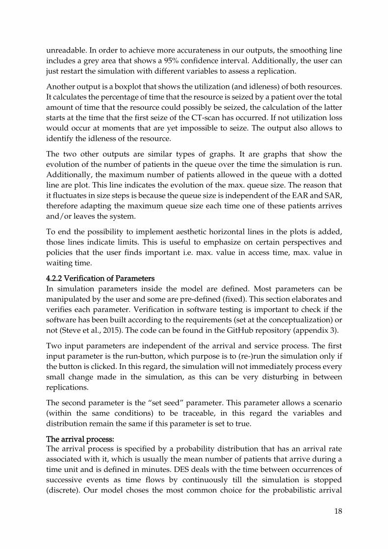
unreadable. In order to achieve more accurateness in our outputs, the smoothing line

includes a grey area that shows a 95% confidence interval. Additionally, the user can

just restart the simulation with different variables to assess a replication.

Another output is a boxplot that shows the utilization (and idleness) of both resources.

It calculates the percentage of time that the resource is seized by a patient over the total

amount of time that the resource could possibly be seized, the calculation of the latter

starts at the time that the first seize of the CT-scan has occurred. If not utilization loss

would occur at moments that are yet impossible to seize. The output also allows to

identify the idleness of the resource.

The two other outputs are similar types of graphs. It are graphs that show the

evolution of the number of patients in the queue over the time the simulation is run.

Additionally, the maximum number of patients allowed in the queue with a dotted

line are plot. This line indicates the evolution of the max. queue size. The reason that

it fluctuates in size steps is because the queue size is independent of the EAR and SAR,

therefore adapting the maximum queue size each time one of these patients arrives

and/or leaves the system.

To end the possibility to implement aesthetic horizontal lines in the plots is added,

those lines indicate limits. This is useful to emphasize on certain perspectives and

policies that the user finds important i.e. max. value in access time, max. value in

waiting time.

4.2.2 Verification of Parameters

In simulation parameters inside the model are defined. Most parameters can be

manipulated by the user and some are pre-defined (fixed). This section elaborates and

verifies each parameter. Verification in software testing is important to check if the

software has been built according to the requirements (set at the conceptualization) or

not (Steve et al., 2015). The code can be found in the GitHub repository (appendix 3).

Two input parameters are independent of the arrival and service process. The first

input parameter is the run-button, which purpose is to (re-)run the simulation only if

the button is clicked. In this regard, the simulation will not immediately process every

small change made in the simulation, as this can be very disturbing in between

replications.

The second parameter is the “set seed” parameter. This parameter allows a scenario

(within the same conditions) to be traceable, in this regard the variables and

distribution remain the same if this parameter is set to true.

The arrival process: The arrival process is specified by a probability distribution that has an arrival rate

associated with it, which is usually the mean number of patients that arrive during a

time unit and is defined in minutes. DES deals with the time between occurrences of

successive events as time flows by continuously till the simulation is stopped

(discrete). Our model choses the most common choice for the probabilistic arrival

19

process: the Poisson process, in which the inter-arrival times of patients are

independent (memoryless) and exponentially distributed with the rate (Zonderland

& Boucherie, 2012). In our simulation, we will let the user switch on/off and

manipulate the inter-arrival time between two patients of the same type. The inter-

arrival times are thus exponentially distributed with = 1/mean inter-arrival time.

As mentioned in the previous section, we consider three types of trajectories. SAR first

seizes a waiting list and then the CT-scan, where UAR and EAR only seize the CT-

scan. The arrival rate of the patients influences the frequency that the patient is

generated, so there is a direct impact at the start of the trajectory. This means that the

inter-arrival times of SAR directly influence the queue (access time) and the seize of

the waiting list. Seizing the waiting list takes a discrete 15 minutes and is fixed for

every SAR, thus the waiting list only releases n amount of appointment slots every 15

minutes. In this regards the number of slots to open influences the arrival rate of SAR

at the CT-scan. The n amount of slots to open equals the amount of SAR (only if enough

SAR are in the system) arriving every 15 minutes. The other arrivals (UAR & EAR) just

arrive according to their inter-arrival times at the CT-scan.

Our model also implements different types of behavior for each type of arrival. We

consider the following phenomena: no-show, balking, and reneging behavior.

SAR have the possibility to not show up. This is indicated by a no-show probability

(uniform distributed) before they seize the CT-Scan. In this regard, the SAR has

successfully finished its place on the waiting list but leaves the system before seizing

the CT-Scan. This means that the appointment slot was reserved for a patient that did

not show up. This utilization loss can be compensated by UAR and EAR who have a

no-show probability fixed at 0%.

Balking behavior refers to UAR patients who will go away (balk) before entering the

queue. Balking only occurs for UAR who decide (for an undefined reason) not to enter

the queue because the queue size in the waiting room is full. Reasons can be that the

facility considers a policy where the max. queue size for unscheduled patients is

defined or that a UAR finds the queue to be too long beforehand.

Reneging behavior refers to UAR patients who will go away (renege) while in queue.

Reasons for reneging behavior can be impatience and/or willingness to wait. Reneging

only occurs if UAR is chosen to be toggled on in the input parameters. To specify the

patience the user can set the reneging behavior in terms of slots. We chose a reneging

distribution that is discrete and occurs after: [𝑖𝑛𝑝𝑢𝑡 𝑛 𝑜𝑓 𝑠𝑙𝑜𝑡𝑠 ∗ 15 𝑚𝑖𝑛𝑢𝑡𝑒𝑠]. We

implement reneging behavior of UAR before seizing the CT-Scan, the behavior is

aborted if the CT-scan has been seized before the selected amount of slots have past.

The service process: The service of the waiting list is fixed at 15 minutes (realizing n scheduled patient

every 15 minutes). The service times of the CT-scan are considered to be normally

distributed. The service times are predefined and therefore the user is unable to

20

manipulate this value. However, the user can manipulate the number of resources

available during the simulation.

The service discipline specifies how incoming patients are served. The discipline we

use for both resources is First Come First Serve (FCFS), where patients are served in

the order of arrival. We do not implement the possibility that SAR can make

appointments at arbitrary moments in time. Therefore we can verify that our

appointment schedule is a combination of two queueing systems for the waiting list

only concerning SAR: M/D/c and for the CT-scan concerning all types: M/M/s/n/∞

Additionally, our model allows for the possibility to include certain policies. By default

SAR and UAR have the same priority while in queue. We implement the possibility to

always help SAR > UAR in the waiting room. By doing so UAR can only be served if

there are no SAR (or EAR) in the waiting room. EAR always has priority over SAR &

UAR, no matter the conditions. Also by default, EAR preempts all current activities,

afterward the preempted activity is restarted. This user can also decide to set

preemption to false.

4.3 User Interface

In this section, we elaborate on the user interface (UI) of the model. The UI allows the

model to be accessible for the user. In chapter 6 we discuss the accessibility of our

application. For reading convenience, we provided a few screenshots in appendix 4.

Our UI interacts from two components. The rendered inputs and the rendered outputs.

For both components, shiny comes with a family of pre-built widgets, each created

with a transparently named R function. Concerning our inputs, we make use of a

function named actionButton that creates an Action Button (run), a function named

NumericInput that creates a numeric input, and a function named sliderInput that

creates a slider bar. Values that are put into these inputs are then sent to the server (the

R model). The R model evaluates the inputs and renders outputs that are consequently

sent to the UI again. The rendered outputs are a family of the following pre-build

widgets. RenderPlots that renders all kinds of plots, renderTables that renders a data

frame, and renderText that renders a print i.e. a summary and/or collection of text

messages.

If we would open all the rendered inputs and outputs into one UI the tool would

become cluttered. Therefore, we adapt and structure the UI. We start by choosing a

neutral background with little variation in colors. From top to bottom we create a UI

with the following elements: title, introduction, inputs, and outputs. To make the user

more aware of the objectives and the inputs we freeze the first three elements. The

output section is divided into a set of tabs (tab panel), the user can click freely through

these tabs. The tabs also include an overview including an example and the operator's

manual.

21

4.4 Verification of the Conceptualization

In the previous chapter, we used the conceptual framework to come up with a

conceptualization. In this section, we will verify to what extent our final model relates

to the desired concept.

Our model successfully verifies and implements all the levels from 0, 1, and the most

of 2. Level 3 was unsuccessfully verified and not implemented. These levels concerned

the following:

▪ Visualization by a moving animation

▪ Implement dynamic appointment scheduling

▪ Interventions during the simulation

▪ Implementation of a scoring system

The visualization of a moving animation is not directly supported in the R language.

Implementing moving objects into our model would require additional programming

language i.e. java. Instead, we choose to include a picture that provides an overview

of the flow of the simulation.

Dynamic appointment scheduling is not implemented. Our simulation supports the

service of arrivals on an FCFS basis. Implementing dynamic appointment scheduling

would require additional literature research and extensive programming adaptations

that we do not consider to be in the scope of our research.

During development, we discovered that simmer only allowed Interventions during

the simulation to be possible if the simulation run was continuous. We choose to

simulate a discrete-event simulation as it allows for a better overview in monitoring

the generated data, which is beneficial for the learning aspect.

We choose not to implement a scoring system. During our development, we decided

that we want to develop a simulation that can be recreated by the user. The purpose is

to see what the influence of selecting certain input parameters have on the outputs.

The consequences can be individually reviewed and outweighed by the user.

Additionally, the operator (who might use the tool during a presentation) could

potentially make it competitive by asking all people in the room to give an estimate.

Therefore we did not include an objective scoring system.

In the next chapter we discuss the accessibility of the tool. Additionally the tool is put

to practice and validated on its input and output parameters.

22

Chapter 5 – Accessibility and validation This section combines steps 2-4 of the game design methodology. It elaborates on the

accessibility of the application and validates the model.

5.1 Accessibility

The user can access the application through the webserver. The website can be visited

under the following URL:

http://sandervandenberg.shinyapps.io/AppointmentScheduler

The website is hosted under a “Free plan” subscription. This comes with some notable

constraints. The ones important for the endurance of our model include:

▪ Active for up to 25 active hours per month. To prevent idle use, we disconnect

the user from our server after not using the application for 5 minutes.

Other functionalities that we cannot include or exclude are:

▪ No password protection on your apps (or other features available only in paid

plans).

▪ Our applications display “Powered by RStudio”.

▪ Up to 5 shiny apps can be hosted – we may archive applications to add new

ones but we will not be able to deploy more than 5. We guarantee that we will

not deploy any other apps at the cost of this application.

5.2 Validation of the model

5.2.1 Validation of the input parameters

We have already verified our parameters in the last chapter. However, we still need to

validate our model. Validation tests how well you addressed the business needs that

caused you to write those requirements. It is also sometimes called acceptance or

business testing. "Did I build what I need?" (Steve et al., 2015).

We validate our model by testing each of the 19 parameters on their extreme (min. and

max.) values and see if the response of the related output is valid. The validation is

traceable (due to parameter 2) and can be checked by any user in the application. It

can also be replicated with other variables to ensure more validity, hence repeating

this scenario is untraceable. The parameter we test is the only parameter that is

manipulated, the others remain their default value. This method can be regarded as a

‘sanity check’ also named a ‘sanity test’. That is a basic test to quickly evaluate whether

a claim or the result of a calculation can be true. In this regard, we quickly check if the

produced material is rational. For reading convenience, we put our results in table III,

as this provides a better overview of the input parameters that are tested.

# Parameter Purpose Use Effect manipulating extreme values

Valid?

1 “run the simulation”.

Running simulation with

Actionbutton that is

The simulation runs accordingly

Yes.

http://sandervandenberg.shinyapps.io/AppointmentScheduler

23

all selected input parameters and producing outputs.

clicked by the user.

and produces different outputs on given inputs as expected.

2 “Play around with the same variables”.

Setting a seed that makes sure that the data and distributions used are traceable.

Checkbox that can be clicked to Boolean values.

If set to true, it remains the same values when re-ran. If false it does not.

Yes.

3 “Allow Unscheduled patients to arrive”

Enables and generates UAR into the system.


If set to true, UAR are found in the plots and tables. False they are not.

Yes.

4 “Allow Emergency patients to arrive”

Enables and generates EAR into the system.


If set to true, EAR are found in the plots and tables. False they are not.

Yes.

5 “Allow for emergency patients to preempt”

Enables EAR to preempt currently used resource.


If set to true EAR do not have a waiting time. If false they do.

Yes.

6 “Allow for priority of Scheduled patients over Unscheduled patients in queue”

Enables SAR to always have priority over UAR in the waiting the room.


If set to true, we find a much higher waiting time for UAR than for SAR. If set to false, it is roughly equal.

Yes.

7 “Allow Unscheduled patients to renege”

Enables UAR to leave the system after n slots.


If set to true (and input slider renege is defined), we see in the ”all patients statistics” that there are UAR in the system with 0 activity time. Which means they left the queueing system without an activity.

Yes.

24

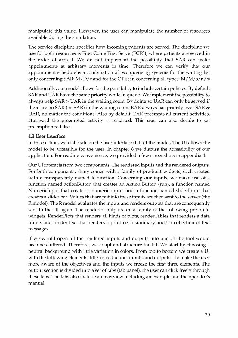
8 “Amount of CT-scan(s)”

Defines the number of resources (servers) that can process an appointment. The more resources, the more patients that can be served.

Sliderbar that can be dragged to a value within a range of selected values.

Min. = 1 leads to an average waiting time of 68. Max. = 3 leads to an average waiting time of 0. Thus there is no queue and always a CT-scan free if n=max.

Yes.

9. “Amount of appointment slots (Scheduled only) to open”

Defines the number of scheduled appointments (only SAR) to open on a single time slot. The more slots to open, the more patients that can make an appointment.


Min = 1 leads to an average access time of 135 and min = 3 leads to an average access time of 50. But waiting time increases. Expected result as more people can make an appointment on a single resource.

Yes.

10. “Amounts of minutes for simulation to Run”

Defines the number of minutes for simulations to run. The longer we run the simulation, the higher the end time will be.


Min = 200 leads to plots with an end time of 200 and if max is 600 leads to plots with end time is 600. The same holds for the logbook and data frames.

Yes.

11 “Inter arrival times Scheduled patients”

Defines the inter-arrival times of SAR. The lower the inter-arrival times the more SAR are generated.


Increasing the inter-arrival times generates less SAR. Min = 2 and generates 172 over 320 min. Max = 8 and generates 42 SAR. Over 320 min. Both are expected values of a Poisson distribution.

Yes.

12 “Inter arrival times

Defines the inter-arrival

Sliderbar that can be

Increasing the inter-arrival times

Yes.

25

Unscheduled patients”

times of UAR. The lower the inter-arrival times the more UAR are generated.

dragged to a value within a range of selected values.

generates less UAR. Min = 5 and generates 59 over 320 min. Max = 55 and generates 7 UAR. Over 320 min. Both are possible values of a Poisson distribution.

13 “Inter arrival times Emergency patients”

Defines the inter-arrival times of EAR. The lower the inter-arrival times the more EAR are generated.


Increasing the inter-arrival times generates less EAR. Min = 50 and generates 6 EAR over 320 min. Max = 150 and generates 4 EAR. Over 320 min. Both are possible values of a Poisson distribution. As the Max is at first sight unlikely we test with parameter 2 disabled, which shows more assumable simulations.

Yes.

14 H-lines in plots Plots a horizontal line for each concerned plot based on a numeric value given by the user. Value of 0 does is expected not to show a line.

Numeric inputbox with a min of 0 (does not show line) and a max of infinite.

We test the three input boxes and see no h-line if the value is 0. If value > 0 a red dotted horizontal line is plotted on the considered plot where the value is provided .

Yes

15 “Amount of Unscheduled patients allowed in queue”

This sets the maximum amount of UAR allowed in the

Sliderbar that can be dragged to a value within a range of

Min = 1. We see that in the All patients stats there is only 1 UAR currently in

Yes.

26

queue to a given value.

selected values.

queue, as it currently has an NA-value in end_time and activity_time. With max=10 there are 3 UAR in the queue as there are no more UAR at the end in the queue (inter arrival times is 25). If we put the parameter at 2. We see a max of 2 again. Balked patients are also not implemented in the graphs and KPI’s (as they should be).

16 “No-show probability of Scheduled patients”

This sets the no show probability of SAR. The appointment slot is reserved for SAR but might they never show up based on a probability given by the user.


If min=0 we find all the 21 finished SAR on the waiting list now either in the waiting room/ at the resource or have successfully finished their appointment. If min=0.25. We find 14 of the total 19 (all patients stats) SAR either in the waiting room/resource or have finished their visit. So 5/19=26% did not show up.

yes

27

No show patients are also not implemented in the graphs and KPIs (as they should be).

17 “Renege of Unscheduled patients after n slots”

If reneging behavior is set to true in 7. We can define the willingness to wait (in terms of slots) of UAR. They leave the system if they cannot seize the resource within the selected number of slots.


We do not test on limits but on a single value. i.e. If we put the input parameter to 2. We expect that the waiting times of UAR that have an activity of 0 (As they reneged) is equal to the amount of slot * duration of slots which is 2*15=30 min. In “all patients stats” we see 10 of these cases. Additionally , UAR with a waiting time of <30 are successfully processed. Thus valid. Reneging patients are also not implemented in the graphs and KPIs (as they should be).

Yes.

Table III Overview of the validation

28

According to our sanity check all of our input parameters are valid. In the next chapter

we validate our outputs. Notice that our outputs are already partly validated in the

current section by testing the input parameters.

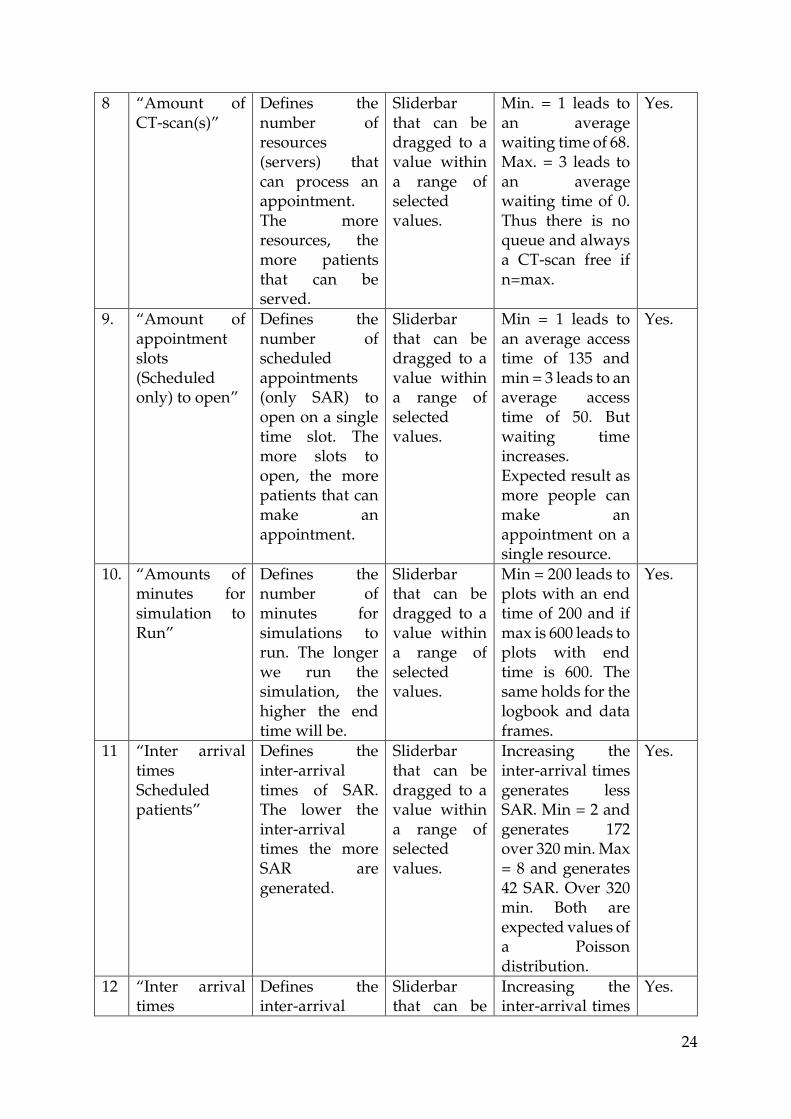
5.2.2 Validation of outputs

We test the outputs with a sanity check. The outputs concern only little variance,

therefore we do not provide an overview in this section.

The main interface consists of 10 outputs. The first output is a graph that shows the

access time of the finished scheduled appointments. This means that it shows the

amount of time that SAR has been on the waiting list before entering the institution.

The graph uses data from the “finished patient statistics”, this data frame is a data

frame that obtains all monitored data (if any) about arrivals and resources. Simmer

does the obtaining for us. Simmer is a valid package in R for simulation. When we

increase the number of appointment slots to open, we see that the average access time

decreases and that the calculations inside that graphs are correctly calculated.

The second graph follows an identical method but this regards the waiting time in the

waiting room before entering the CT-scan and considers all patient types.

Both the first two graphs show a confidence interval – grey area - of 95%, we choose

to implement this because we do not do any replications inside the simulation.

Additionally, the smooth line has a degree of 2 that indicates the degree of the

smoothing line between the points in the plots. If the degree is higher than the number

of unique points, we will get a computation fail. Therefore in some cases, we will not

see a smoothing line including the confidence interval.

The third graph is a boxplot that shows the utilization of both resources. It calculates

the percentage of time that the resource is seized by a patient over the total amount of

time that the resource could possibly be used, the calculation of the latter starts at the

time that the first seize of the CT-scan has occurred. If we would not do this we would

have utilization loss even though that there already are scheduled patients in the

system. We test this by putting all interarrival times at the max. and put the number

of CT-scan at max. In this regard, we have a lesser arrival rate than the service rate and

thus the utilization is disastrously low (42 %). When we put the input parameters to

their min. values the opposite occurs and we find utilization of 100%.

The fourth and the fifth outputs show similar types of graphs. It shows the evolution

of the number of patients in the queue over the time the simulation is run. This graph

is similarly tested as the third graph. As a decreasing service rate (n of CT-scans)

correctly increase the number of patients in queue. Consequently, increasing the

service rate decreases the number of patients. Additionally, it shows a dotted line

indicating the max. amount of patients allowed in the queue. We see that the dotted

line starts at the max amount indicated in the parameter. SAR and EAR both increase

and decrease by 1 depending on the activity (arrival or release). This is indeed the case

at the moments in the time that they arrive and leave the system as can be seen in

“patients stats”.

29

The 6th output is a textbox that is supposed to show the logbook – indicates what is

happening – and the summary of the simulation. Rendering both objects is a valid

function within the simmer package. However, when we run the simulation, the

logbook is not always included. This is concerned to be an unsolved bug within the

interactivity of Rshiny and the Simmer package. As the correct outputs are always

correctly printed in the console of Rstudio but not in our reactive environment. Luckily

the model can still be operationalized without the use of the logbook. Additionally

simmer always generates one “dummy patient”. This “dummy patient” is included in

the summary but not in the plots and data frames. In this regard, the n patient types

generated in our simulation are always 1 less than the summary shows the user.

The other 4 outputs all concern data frames that are gathered through simmer. The

data collected by simmer is not tested since they are already concerned to be valid as

they are part of the simmer package. The only difference in the data frames is that the

“all finished statistics” only concerns finished patients (successfully released patients)

where the “all patient statistics” concerns all patients excluding balked UAR, as they

have never entered the system. We add two columns that calculate the access and

waiting time. Both KPIs are calculated with the following formula: 𝑊𝑎𝑖𝑡𝑖𝑛𝑔 𝑡𝑖𝑚𝑒/

𝑎𝑐𝑐𝑒𝑠𝑠 𝑡𝑖𝑚𝑒 = [𝐸𝑛𝑑 𝑡𝑖𝑚𝑒 – (𝑠𝑡𝑎𝑟𝑡 𝑡𝑖𝑚𝑒 + 𝑎𝑐𝑡𝑖𝑣𝑖𝑡𝑦 𝑡𝑖𝑚𝑒)]. We discover that both

KPIs sometimes have negative values (e-15) that approach 0. The reason is that the

data in the calculation is gathered by simmer and has some rounding errors. As these

values approach 0, the error is negligible.

We can conclude that most outputs are successfully validated. We could not change

the minor invalid aspects in our outputs, the only option was entirely disabling the

output. The minor invalid aspects are not disastrous to the use of our model (as can be

seen in chapter 6), therefore we decided to include them and notify the user.

5.3 Limitations and assumption of the model

5.3.1 Limitations

In our verification and validation, we elaborate on the choices, bugs, and errors of our

model. In this section we summarize the limitations:

▪ Replications: We choose not to implement replications as the logbook and the

readability of the plots would become cluttered. Replications can still be

achieved by re-running the simulation.

▪ Simulation loss at the start: In the first 15 minutes, SAR can not join the CT-scan

as they first need to have an appointment. Simmer did not allow to start the

simulation from 15 seconds. Therefore, we set the calculations of all outputs to

begin when the first patient arrives.

▪ Negative values in calculations access and waiting time: Negative values

approaching 0 are possibly calculated because of rounding errors.

▪ RenderPrint error: Simmer and Rshiny have a bug that at arbitrary moments,

not all printed logs are included.

30

▪ Computation stat smooth failed: If the degree is lower than the number of

unique points. We will not see a smoothing line (and confidence interval)

between the points in the first two plots. The mean is still calculated.

▪ Sum of n_generated: The dummy generated is included in the summary,

therefore there is actually one less patient (of each type) generated as the

summary shows us.

5.3.2 Assumptions:

There assumption that we consider is that the population of potential patients will be

assumed to be infinite, even though in reality the number of potential patients is

actually finite (the K in the queuing notation). The assumption of an infinite population

is such that the rate of arrival of patients is not affected by the number of patients that

have already joined the queuing system. In addition, this will usually entail that the

rate of arrival is constant throughout time.

Also, the resources are identical. They are distributed equally. Patients can be helped

by both resources and join the same queue, hence they do not pool.

31

Chapter 6 - Experimentation This section elaborates on stage IV and V of the game design methodology. This

concerns the prototyping and the operator's manual of the serious game.

Experimentation

In this section, we validate the model on their learning objectives by testing two

scenarios. Scenario (i) is concerned to be a fictional scenario based on our own

assumptions. Scenario (ii) is a case study at the AMC. This case study uses real data

assessed by (Kortbeek et al., 2014) to test his iterative procedure discussed in the

source. In this regard, we try to replicate the institutions their conditions into our

model. The scenarios can be recreated by putting the same parameters into our model.

Experiment 1: Facility X

In experiment 1 we want to test the influence of the amounts of slots open for

appointment scheduling during one day (6 hours) at facility X. We consider facility X

to have the policy to keep the access time as low as possible (patient perspective) while

keeping the utilization of the CT-scan(s) not under 80% (hospital perspective). We

consider the following parameters.

Parameter Description Value

n Number of Resources (CT-Scan) 1

a Appointment slots to open C(1,2,3)

1/SAR Interarrival times of Scheduled patients for waiting list 5 min

1/UAR Interarrival times, if any, of Unscheduled patients for waiting room

15 min

1/EAR Interarrival times, if any, of Emergency patients for waiting room

100 min

P Preemptive priority Emergency patients (boolean) True

R Amount of unscheduled patients allowed in waiting Room 3

q No-show probability of Scheduled patients 0.05 %

Z Allow for priority of Scheduled patients over Unscheduled patients in queue

False

Y Allow Unscheduled patients to renege False

Run Amounts of minutes for simulation to Run 320 min

The fixed parameters are:


S Service times of CT-scan rnorm(15,1)

T Timeslots 15 min

The UI is set to the the parameters above, these parameters influence the simulation

model. Before we run the simulation, we click the option “Play around with same

32

variables”. This “sets a seed” and makes sure that our random generated values are

traceable. Hlines are aesthetic and not of importance.

We test the Parameter “Appointment slots to open” on all three values {1,2,3}. We

hypothesize that the waiting room will become cluttered the more slots are opened.

The reasons are that more fixed appointments are being made on a single resource

with a fixed service time. Consequently, the access time will be decreased as the

number of slots opened increases.

Below the outputs are summarized. Only finished arrivals per resource are taken into

account in the calculation of the KPIs.

1. If only one appointment is made every 15 minutes, we find an average access

time of 119 minutes for 21 SAR. Hence, there are still 36 patients on the waiting

list. The average waiting time in the waiting room is 67 minutes for 19 patients

(of all types). Hence, there are still 13 patients in the waiting room. CT-Scan is

finished by 10 SAR, 6 UAR, and 3 EAR. The utilization of the CT-scan is 100%.

2. If two appointments are made every 15 minutes, we find an average access time

of 90 minutes for 41 SAR. Hence, there are still 26 patients on the waiting list.

The average waiting time in the waiting room is 88 minutes for 19 patients (of

all types). Hence, there are still 34 patients in the waiting room. CT-scan is

finished by 11 SAR, 5 UAR, and 3 EAR. The utilization of the CT-scan is 100%.

3. If three appointments are made every 15 minutes, we find an average waiting

access time of 40 minutes for 59 SAR. Hence, there are still 8 patients on the

waiting list. The average waiting time in the waiting room is 99 minutes for 19

patients (of all types). Hence, there are still 49 patients in the waiting room. The

CT-scan is finished by 12 SAR, 4 UAR, and 3 EAR. The utilization of the CT-

scan is 100%.

Scenario Appointment slot

Avg. access time. (min)

avg. Waiting time (min)

n SAR still on waiting list

n still in waiting room

Utilization in CT(%)

1 1 4179/21=119 1273/19=67 36 13 100

2 2 3690/41=90 1672/19=88 26 34 100

3 3 2360/59=40 1881/19=99 8 49 100

The output shows that the strategy of facility X is to open 3 appointment slots. In this

strategy, the access time is the lowest, while the utilization is at 100%. However, but

not of importance in this policy, this strategy does allow that the waiting room to

become cluttered and accept a higher waiting time. Keep in mind that in this

calculation only the finished patients are taken into account, so the waiting time will

only increase more the longer simulation is run. In this regard, we conclude that our

hypothesis is correct.

33

Experiment 2: CT-Scan AMC

In experiment 2 we are inspired by the Case Study conducted by N. Kortbeek

(Kortbeek et al., 2014). We implement some of the parameters provided (underlined)

in the case and make assumptions where this is not possible. In this scenario, we do

no consider a policy, but we analyze the influence of the no-show probability of SAR

on the service of UAR on the model. We vary the interarrival times of UAR and the

no-show probability.

The following parameters are concerned:


n Number of Resources (CT-scan) 2

a Appointment slots to open 2

1/SAR Interarrival times of Scheduled patients for waiting list 5

1/UAR Interarrival times, if any, of Unscheduled patients for waiting room

C(43,0)

1/EAR Interarrival times, if any, of Emergency patients for waiting room

0 (False)

P Preemptive priority Emergency patients (boolean) False

q No-show probability of Scheduled patients C(0.05, 0.10,0.20)

R Amount of unscheduled patients allowed in waiting Room 5

Y Renege after, if any, amount of slots for Unscheduled patients

c(Null, 2)

Z Allow for priority of Scheduled patients over Unscheduled patients in queue

True

Run Amounts of minutes for simulation to Run 510 min

According to the case, the initial demand for unscheduled services per week is cyclic

and has an average of 11,86 per day over 5 days. In the procedure they consider

reserved time slots for the specific arrivals and their demands, we do not provide this

possibility in our research. Therefore, we say that the interarrival time is 510/11,86=43

min for unscheduled arrivals. The scheduled arrivals (1 every 5 min) are generated so

that there are always enough patients on the waiting list. The queue priority is given

to SAR so that a UAR can only seize the resource when the SAR does not show up. In

the case a survey reveals that patients are willing to wait no more than 2 slots. The

simulation is run from 8:00 to 16:30 (34 slots).

The fixed parameters are:


S Service times of CT-scan rnorm(15,1)

T Timeslots 15 min

We click the option “Play around with same variables” again. The access time is not of

importance in this scenario. Due to the priority, we only consider the waiting time of

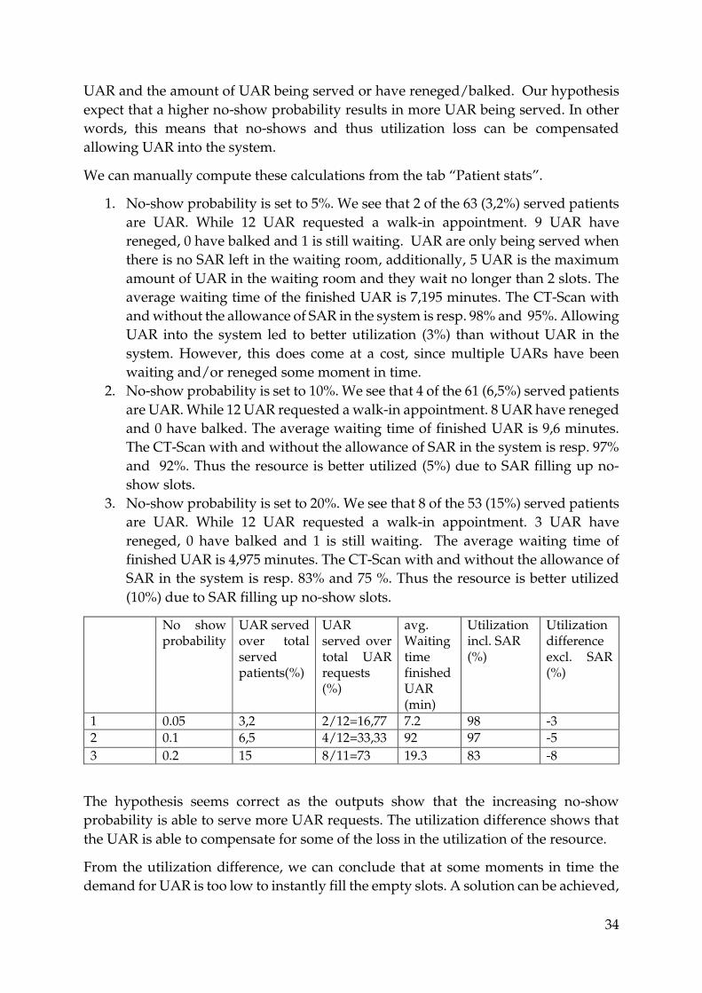
34

UAR and the amount of UAR being served or have reneged/balked. Our hypothesis

expect that a higher no-show probability results in more UAR being served. In other

words, this means that no-shows and thus utilization loss can be compensated

allowing UAR into the system.

We can manually compute these calculations from the tab “Patient stats”.

1. No-show probability is set to 5%. We see that 2 of the 63 (3,2%) served patients

are UAR. While 12 UAR requested a walk-in appointment. 9 UAR have

reneged, 0 have balked and 1 is still waiting. UAR are only being served when

there is no SAR left in the waiting room, additionally, 5 UAR is the maximum

amount of UAR in the waiting room and they wait no longer than 2 slots. The

average waiting time of the finished UAR is 7,195 minutes. The CT-Scan with

and without the allowance of SAR in the system is resp. 98% and 95%. Allowing

UAR into the system led to better utilization (3%) than without UAR in the

system. However, this does come at a cost, since multiple UARs have been

waiting and/or reneged some moment in time.

2. No-show probability is set to 10%. We see that 4 of the 61 (6,5%) served patients

are UAR. While 12 UAR requested a walk-in appointment. 8 UAR have reneged

and 0 have balked. The average waiting time of finished UAR is 9,6 minutes.

The CT-Scan with and without the allowance of SAR in the system is resp. 97%

and 92%. Thus the resource is better utilized (5%) due to SAR filling up no-

show slots.

3. No-show probability is set to 20%. We see that 8 of the 53 (15%) served patients

are UAR. While 12 UAR requested a walk-in appointment. 3 UAR have

reneged, 0 have balked and 1 is still waiting. The average waiting time of

finished UAR is 4,975 minutes. The CT-Scan with and without the allowance of

SAR in the system is resp. 83% and 75 %. Thus the resource is better utilized

(10%) due to SAR filling up no-show slots.

No show probability

UAR served over total served patients(%)

UAR served over total UAR requests (%)

avg. Waiting time finished UAR (min)

Utilization incl. SAR (%)

Utilization difference excl. SAR (%)

1 0.05 3,2 2/12=16,77 7.2 98 -3

2 0.1 6,5 4/12=33,33 92 97 -5

3 0.2 15 8/11=73 19.3 83 -8

The hypothesis seems correct as the outputs show that the increasing no-show

probability is able to serve more UAR requests. The utilization difference shows that

the UAR is able to compensate for some of the loss in the utilization of the resource.

From the utilization difference, we can conclude that at some moments in time the

demand for UAR is too low to instantly fill the empty slots. A solution can be achieved,

35

by generating more UAR (increasing demand) or disabling/increasing the reneging

behavior. However, this comes as at a cost, as manipulating these parameters can lead

to high waiting times for unscheduled patients.

Learning context

This section elaborates on the learning context. In the first experiments we see the

influence of the “appointment slots to open” and in the second we see the influence of

the ”no-show probability” on the simulation. Many other different experiments are

feasible. It depends on what the user find interesting to inspect, hence the goal remains

the same: Use the tool to simulate a hospital environment and adapt input parameters

to enhance the relation between the parameters.

With this goal in mind, the player is challenged to play and understand the following

steps:

1. Create a hospital environment with the input parameters

2. Run the simulation

3. Inspect the output parameters.

4. Decide for goal: what do you want to change in the output parameters?

5. Make a decision: What input parameter do we want to influence?

6. Apply different scenarios to the input parameters

7. Inspect the output parameters

8. Draw conclusions

9. Repeat step 1-6 with a different parameter

By following these steps the user is stimulated to understand the influence of a certain

input parameter on the simulation. If adaptations of this parameter benefit the

intended goal, then measures can be executed to put the adaptation to practice.

36

Chapter 7 - Conclusion & discussion Values for science: In this thesis, we have outlined the development of a serious game. This thesis

concerns a design approach rather than a problem-solving approach. The

development is twofold: developing a serious game and outlining the concept of

appointment scheduling. We successfully combined both elements by following the

combination of two methodologies: the conceptual framework for simulation-based

serious games and the game design methodology.

The first methodology shaped our conceptualization (why, how, what). Where the

other methodology concerned the overall game design (from development to

experimentation). These methodologies have also served as the pillar of the divisions

of chapters, sections, and subsections.

At first sight, our visualization tool looks more like a simulation. However, in our

simulation, the user is able to respond and manipulate the process. In this regards the

user is able to learn more about a particular concept by active learning. Therefore, we

can conclude that our simulation falls into a taxonomy within serious games but only

includes little gaming aspects i.e. no way to obtain a high score, competition with other

players. Our serious game however is more an interactive tool that expresses itself

through active learning with trial and error. As the user can freely play around with

input parameters and see what the influence of his actions are on the output

parameters. In this regard, the user can draw his own conclusions and anticipate them

in the next simulation. Also, an operator (who has experience in using the tool) can

make it competitive by letting an audience decide on an estimate during a presentation

for example.

Concerning the modeling objectives, we find our game to be useful in analyzing the

relationship between parameters. The objective of the serious game is to simulate a

hospital by deciding on the input parameters. Chapter 7 concerns experimentation in

which we explain the potential of the game and where we successfully defend our

hypotheses. Therefore, we also conclude an example of this experimentation into our

model, so that can emphasize the modeling objectives to the user.

The pedagogic purposes concern the main learning objective and that is to create more

intuition about appointment schedule systems. We want the user of the serious game

to realize the potential of this mixed appointment system in healthcare. We emphasize

the contrast as we compare traditional options (scheduled only) to a mixed system.

Values for practice:

We verified and validated the model on its parameters. Together with the conclusion

of our objectives, our serious game offers the possibility to create a better

understanding in appointment scheduling. Only few serious games in healthcare

currently exist and extension to the application are feasible. Extensions can be dynamic

scheduling systems, implementing a scoring aspect. Incorporations as such lead to

37

more dynamic serious games. Also, we successfully applied an existing conceptual

framework for simulation based serious gaming therefore it delivers a contribution in

the field of serious games. However, the application has not yet been tested by

professionals and therefore we cannot determine the value that the tool has in practice.

Further research:

It is still hard to determine if the pedagogic purposes are met. This would require

additional research in the evaluation, which we do not include in the scope of this

research. Also many improvements are possible. Further research can determine if

there are more options within the taxonomy of serious games possible. At last, there

are a lot of similar concepts within OM (i.e. pooling effect, integral capacity

management) that contribute to the same pedagogic purpose, these concepts can also

be visualized.

38

References Allen, M., Spencer, A., Gibson, A., Matthews, J., Allwood, A., Prosser, S., & Pitt, M. (2015).

What is discrete event simulation, and why use it? https://www.ncbi.nlm.nih.gov/books/NBK293948/

Borgman, N. J., Vliegen, I. M. H., Boucherie, R. J., & Hans, E. W. (2018). Appointment scheduling with unscheduled arrivals and reprioritization. Flexible Services and Manufacturing Journal, 30(1), 30–53. https://doi.org/10.1007/s10696-016-9268-0

Cayirli, T., & Veral, E. (2009). Outpatient scheduling in health care: A review of literature. Production and Operations Management, 12, 519–549. https://doi.org/10.1111/j.1937-5956.2003.tb00218.x

DataFlair. (2019). Why Learn R? 10 Handy Reasons to Learn R programming Language. In DataFlair. https://data-flair.training/blogs/why-learn-r/

Greenblat, C. S., & Duke, R. D. (1981). Principles and Practices of Gaming-Simulation. SAGE Publications. https://books.google.nl/books?id=EvVOAAAAMAAJ

Günal, M. M., & Pidd, M. (2010). Discrete event simulation for performance modelling in health care: A review of the literature. Journal of Simulation, 4(1), 42–51. https://doi.org/10.1057/jos.2009.25

Gupta, D., & Denton, B. (2008). Appointment scheduling in health care: Challenges and opportunities. IIE Transactions, 40, 800–819. https://doi.org/10.1080/07408170802165880

Holleman, D. R., Bowling, R. L., & Gathy, C. (1996). Predicting daily visits to a walk-in clinic and emergency department using calendar and weather data. Journal of General Internal Medicine, 11(4), 237–239. https://doi.org/10.1007/BF02642481

Jantke, K. P. (2010). Toward a taxonomy of game based learning. Proceedings of the 2010 IEEE International Conference on Progress in Informatics and Computing, PIC 2010, 2, 858–862. https://doi.org/10.1109/PIC.2010.5687903

Kortbeek, N., Maartje, ;, Zonderland, E., Braaksma, A., Vliegen, I. M., Richard, ;, Boucherie, J., Litvak, N., & Hans, E. W. (2014). Elsevier Editorial System(tm) for Performance Evaluation Manuscript Draft Manuscript Number: PEVA-D-12-00186R2 Title: Designing Cyclic Appointment Schedules for Outpatient Clinics with Scheduled and Unscheduled Patient Arrivals Article Type: SI: Service Science of Queues.

Laamarti, F., Eid, M., & El Saddik, A. (2014). An overview of serious games. International Journal of Computer Games Technology, 2014(May 2016). https://doi.org/10.1155/2014/358152

Lope, R. P. De, & Medina-Medina, N. (2017). A Comprehensive Taxonomy for Serious Games. Journal of Educational Computing Research, 55(5), 629–672. https://doi.org/10.1177/0735633116681301

News, I. (2015). Serious Games A 10 billion euro market in 2015 (Vol. 33, Issue July 2010, pp. 5–7). https://www.seriousgamemarket.com/2010/08/idate-serious-games-10-billion-euro.html

39

Pohlmann, U., Schäfer, W., Reddehase, H., Röckemann, J., & Wagner, R. (2012). Generating Functional Mockup Units from Software Specifications.

Quinn, C., & Neal, L. (2008). Serious games for serious topics. In eLearn (Vol. 2008, Issue 3). https://doi.org/10.1145/1361083.1361093

Riedel, J. C. K. H., & Hauge, J. B. (2011). State of the art of serious games for business and industry. 2011 17th International Conference on Concurrent Enterprising, 1–8.

Robinson, S. (2008). Conceptual modelling for simulation Part I: definition and requirements. Journal of the Operational Research Society, 59(3), 278–290. https://doi.org/10.1057/palgrave.jors.2602368

Shin, Y. W., & Choo, T. S. (2009). M/M/s queue with impatient customers and retrials. Applied Mathematical Modelling, 33(6), 2596–2606. https://doi.org/https://doi.org/10.1016/j.apm.2008.07.018

Sickinger, S., & Kolisch, R. (2009). The performance of a generalized Bailey-Welch rule for outpatient appointment scheduling under inpatient and emergency demand. Health Care Management Science, 12, 408–419. https://doi.org/10.1007/s10729-009-9098-7

Steve, A., Policy, M., & Posts, P. (2015). The difference between Verification and Validation 29. (pp. 11–14). https://smartbear.com/blog/verification-and-validation-the-difference/

Van Der Zee, D. J., Holkenborg, B., & Robinson, S. (2012). Conceptual modeling for simulation-based serious gaming. Decision Support Systems, 54(1), 33–45. https://doi.org/10.1016/j.dss.2012.03.006

Zhang, X. (2018). Application of discrete event simulation in health care: A systematic review. BMC Health Services Research, 18(1), 1–11. https://doi.org/10.1186/s12913-018-3456-4

Zonderland, M. E., & Boucherie, R. J. (2012). Queuing networks in healthcare systems. International Series in Operations Research and Management Science, 168, 201–243. https://doi.org/10.1007/978-1-4614-1734-7_9

Zyda, M. (2005). From visual simulation to virtual reality to games. Computer, 38(9), 25–32. https://doi.org/10.1109/MC.2005.297

40

Appendices Appendix 1: Criteria of the taxonomy

Elaboration of the five criteria in the taxonomy

2.2.1. The first criteria is about the activity performed by the user and is required by

the game. In literature, they define it as the function – physical, mental, etc. - performed

as a response or input to the game. In our case, we will likely focus on the mental

aspect, as we would want to emphasize the learning aspect by education.

2.2.2. Another criterion is the importance of modality, which is the channel by which

information is communicated from the computer to the human(s) participating in the

game. This characterizes the sensory modalities the player experiences in the game.

The most common modalities include visual, auditory, and haptic. In our case, we will

likely focus on the visual aspect.

2.2.3. The criterion of interaction style defines whether the interaction of the player

with the game is done using traditional interfaces such as keyboard, mouse, or

Joystick. But could also be using some intelligent interface such as a brain interface,

eye gaze, movement tracking, and tangible interfaces. In our case, we will likely keep

I t more simplistic and focus on interaction from keyboard and mouse.

2.2.4. This criterion defines the environment of the digital game and can be a

combination of several criteria Considering this theory, the environment that our

application will likely be in includes the following aspects in order of the source:

single/multiplayer, two-dimensional, reality environment, location unawareness,

mobile and online accessible.

2.2.5. The application area refers to the different applications domains relevant to

serious games. There are many possible application areas. In our case, this would be

the application area of education and healthcare.

Appendix 2: Outline of the conceptual framework for simulation-based gaming

This summary is derived from the paper by (Van Der Zee et al., 2012)

2.3.1. Understanding the learning environment

The game designer’s notion and understanding of the learning environment is a

prerequisite for developing an adequate game. This understanding involves subject

matters, client interests, education backgrounds, the interest of the prospective players

and operates, and the context of use.

Therefore we start by researching the subject matters. The subject matters are the core

of the learning environment. An understanding of the learning environment creates

the starting point for determining modeling objectives. The learning environment has

to make an awareness of the learning needs. We relate the notion of computer-based

games to the use of simulation models for representing real-world operations systems.

Simulation tools offer large flexibility in their realistic modeling of operations systems

in various levels of detail, thereby serving the interests of various player groups.

41

However, such flexibility comes at a price – model set-up may involve significant

investments in terms of resources, time, and money.

2.3.2. Determine modeling and general project objectives

The learning environment sets the contours for game and simulation model

development. To start game development, this knowledge needs to be linked to the

game's pedagogic purpose(s)1. Modeling objectives can be expressed in terms of

players' achievements in mastering their decision-making skills. Typically, players'

decision-making skills are linked to their notion and interpretation of system status,

and their maturity in choosing among decision options – given some criteria for

optimization. For example, the simulation model is to facilitate players' learning on

improving to balance the access and waiting within the institution. It is important that

these objectives can be met in resource availability. For example, to cut the expenses

in game development, and to meet the project timeline, decreasing model detail may

seem a viable option. In this manner, you set a limit to the extensive options within

your game. A simpler model does not necessarily mean a bad model as simpler models

may be acceptable in an educational context, where model precision may be varied to

some extent.

It is important to combine these objectives with effective player interaction. Van der

zee mentions 4 points to consider:

▪ Model visualization: how to display model entities and their detail (2D, 3D,

schematic, iconic)?

▪ Model interaction (game interface, simulation model interface): how to facilitate

players'/ operators' interaction with the model (dragging, pop-ups, menus,

error reports, help functions)?

▪ Model responsiveness: what delays (execution times) are acceptable for the

model's responses to players' decisions?

▪ Model reuse: how easily can the model accommodate alternative groups of

players, with possibly different backgrounds?

2.3.3. Identify the model outputs

Model outputs have two purposes. The first is to indicate players' achievements

relative to the pedagogic purposes set and secondly to emphasize the players'

achievements. In most cases, those responses indicating players' achievements can be

derived from the modeling objectives in chapter 4. The output can be seen as the

response that seeks to link system operations and player decision-making with

players' achievements. In simulation, tools do not offer standard features for tracing

player decision-making. As most simulations render outputs from pre-set options.

Once the required model outputs are identified, we decide on the way they are

presented to the player. Formats to present include numerical data (i.e. mean,

1 What a player should have learned after completing the game

42

minimum, maximum, standard deviation) or graphical reports (i.e. time series, bar

charts, Gantt charts). As long as these choices of format are in line with the project

objectives.

2.3.4. Identify the model inputs

Model inputs are linked to operator inputs, allowing the user to intervene in the game

set-up and manipulate the simulation process. The choice of model inputs determines

the way the model may be tailored to reflect alternative system configurations, initial

system status, or assumptions on factors external to the system. Model inputs can be

altered with buttons, sliders, and so forth. In applications, it is not hard to allow

altering of model inputs, with possibly wide ranges. But they should contribute to the

functionality of the game. Therefore we carefully consider the contribution of the

inputs to the game utility (the “right” game settings), and its feasibility (“not too many

games”). A careful choice of inputs is therefore required, starting from the modeling

objectives, player availability, resources, and game format.

2.3.5.

Determining the model its content entails two activities: scope and level of detail. The

scope of the Model identifies the model boundaries in terms of components to be

included in the model, whereas model detail establishes model depth in terms of

components' attributes. To identify the components, a three-step approach is

proposed: (i) Identify the system boundary, (ii) Identify components within the

boundary, and (iii) Assess whether to include/exclude all components identified.

After deciding on the components to include in the model, their detail has to be

determined. The framework suggests that, for model scope, decisions should be

recorded on model detail using tables and/or diaendigrams, characterizing and

justifying the detail for each model component.

Additionally, both activities go together with simplifications assumptions. Here

assumptions follow from uncertainties about the referent system, whereas

simplifications are meant to make model development and use easier.

The Conceptual framework is evaluated and judged on its quality on four different

criteria. Validity, Credibility, utility, and feasibility Following the judgment on the

criteria van der Zee his conceptual framework were determined to be appropriate as a

conceptual model. In this regard, we will apply the modeling framework for the

conceptualization of our model.

Appendix 3: URLs to tools and codes

Tiox tool: https://tiox.org/stable/index.html#que

Control widgets: https://shiny.rstudio.com/tutorial/written-tutorial/lesson3/

Application/Serious game:

https://sandervandenberg.shinyapps.io/AppointmentScheduler/

https://tiox.org/stable/index.html#que

https://shiny.rstudio.com/tutorial/written-tutorial/lesson3/

https://sandervandenberg.shinyapps.io/AppointmentScheduler/

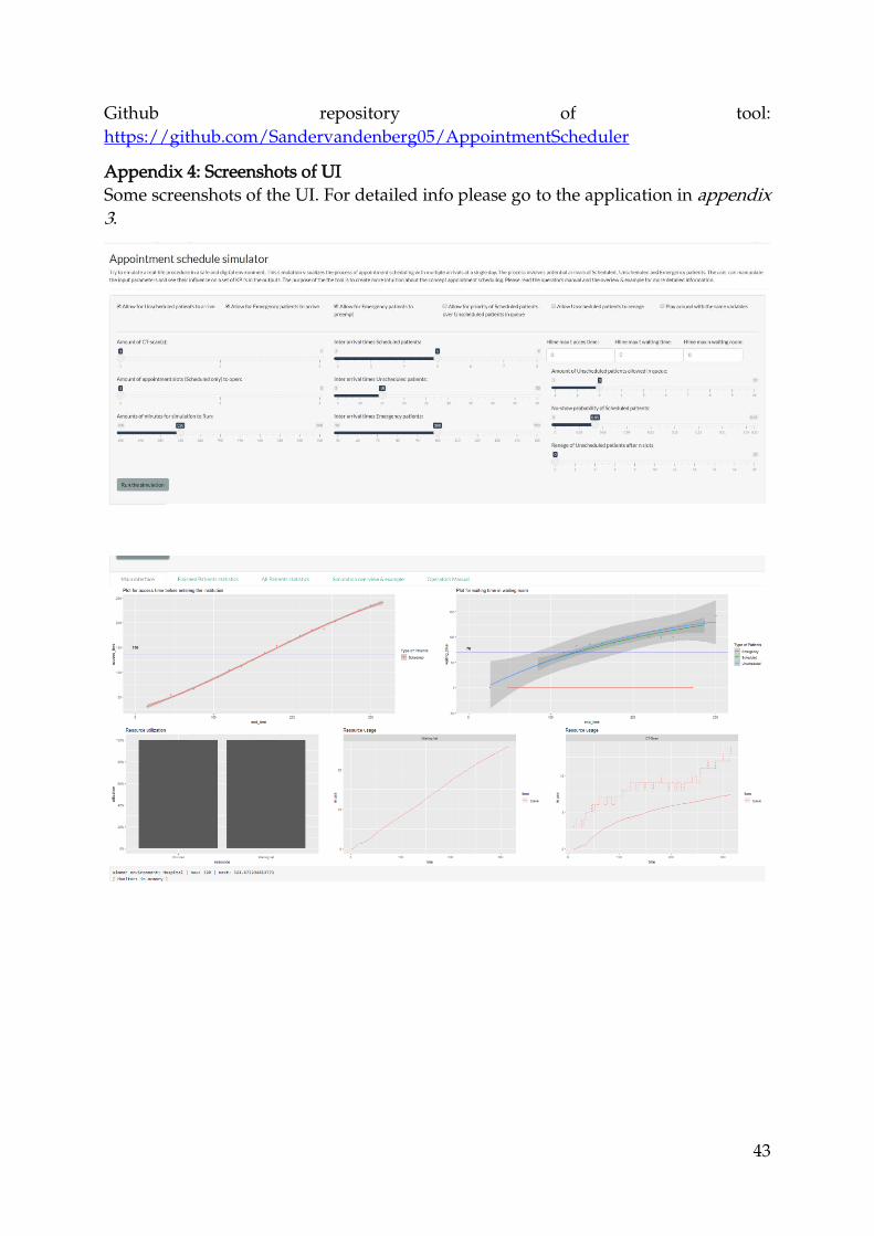
43

Github repository of tool:

https://github.com/Sandervandenberg05/AppointmentScheduler

Appendix 4: Screenshots of UI

Some screenshots of the UI. For detailed info please go to the application in appendix

3.

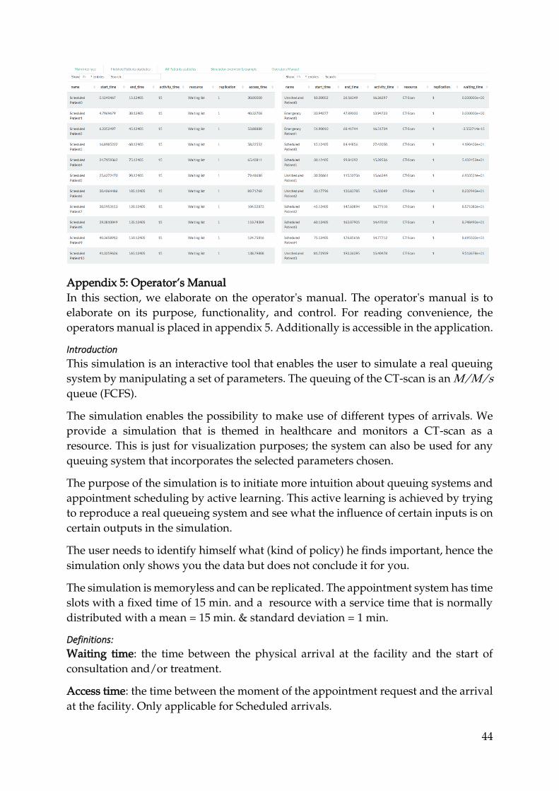
https://github.com/Sandervandenberg05/AppointmentScheduler

44

Appendix 5: Operator’s Manual

In this section, we elaborate on the operator's manual. The operator's manual is to

elaborate on its purpose, functionality, and control. For reading convenience, the

operators manual is placed in appendix 5. Additionally is accessible in the application.

Introduction

This simulation is an interactive tool that enables the user to simulate a real queuing

system by manipulating a set of parameters. The queuing of the CT-scan is an M/M/s

queue (FCFS).

The simulation enables the possibility to make use of different types of arrivals. We

provide a simulation that is themed in healthcare and monitors a CT-scan as a

resource. This is just for visualization purposes; the system can also be used for any

queuing system that incorporates the selected parameters chosen.

The purpose of the simulation is to initiate more intuition about queuing systems and

appointment scheduling by active learning. This active learning is achieved by trying

to reproduce a real queueing system and see what the influence of certain inputs is on

certain outputs in the simulation.

The user needs to identify himself what (kind of policy) he finds important, hence the

simulation only shows you the data but does not conclude it for you.

The simulation is memoryless and can be replicated. The appointment system has time

slots with a fixed time of 15 min. and a resource with a service time that is normally

distributed with a mean = 15 min. & standard deviation = 1 min.

Definitions:

Waiting time: the time between the physical arrival at the facility and the start of

consultation and/or treatment.

Access time: the time between the moment of the appointment request and the arrival

at the facility. Only applicable for Scheduled arrivals.

45

Preemptive: Preempt at true allows for Emergency patients to stop a current activity,

which is later restarted.

Renege: This allows the player to leave while in queue.

Input Parameters

1. Enables and generates Unscheduled arrivals into the system.

2. Enables and generates Emergency arrivals into the system.

3. Enables emergency patient to preempt currently used resources.

4. Enables Scheduled patients to always have priority over unscheduled patients

in the waiting room.

5. Enables Unscheduled patients to leave the system after n slots

6. Setting a seed that make sure that the data and distributions used are traceable..

7. Defines the number of resources (servers) that can process an appointment.

8. Defines the number of scheduled appointments to open on a single time slot.

9. Defines the number of minutes for simulation to run.

10. Define inter-arrival times of patients that are Poisson distributed (exponential

with rate = 1/inter arrival times)

11. Plots a horizontal line for each concerned plot based on a numeric value given

by the user. Value of 0 does is expected not to show a line.

12. This sets the maximum number of Unscheduled patients allowed in the queue

to a given value.

13. This sets the no-show probability of Scheduled arrivals. The appointment slot

is given free to the other two potential arrivals waiting.

14. If reneging behavior is set to true in (5) we can define the willingness to wait (in

terms of slots) of Unscheduled Patients. They leave the system if they cannot

seize the resource within the selected number of slots.

Outputs

Main interface:

1. Access time plot: Graph that shows the access times of all scheduled patients

finished from the waiting list (dots) and calculates the average access time of all

finished patients on the blue horizontal line. Includes a gray area to show a 95%

confidence interval in values.

2. Waiting time plot: Graph that shows the waiting times of all types of patients

(in the waiting room) that have successfully used the CT-Scan. Idem. Visual

aspects idem. as 1.

46

3. Resource utilization: Boxplot that shows the utilization and idleness of both

resources.

4. Resource usage waiting list: This shows the evolution of the number of

scheduled patients on the waiting list.

5. Resource usage CT-scan: This shows the evolution of the number of all patients

inside the waiting room, the dotted line represents the maximum number of

patients allowed in queue at a moment in time.

6. Either provides a summary of the simulation or provides a logbook that shows

what is happening inside the simulation.

Finished Patient statistics:

1. Provides a data frame that collects all the data of the simulation for finished

patients. This data frame is also the underlying data used by the plots in the

main interface.

All Patient statistics:

1. Provides a data frame that collects all the data of the simulation for finished

patients. This data frame can be used to analyze unsuccessfully (balked,

reneged, or waiting) finished patients.

Simulation overview & statistics:

1. Simulation overview that provides a picture of the simulation. It also elaborates

by use of one example. The example contain the default values that are selected

at the initial start of the simulation.

Screenshot of Manual in application

47

Additional figures

These figures are put in the appendix because they are too big or too disturbing in text.

Figure IV Summary of the Game Design (Greenblat & Duke, 1981)

48

Figure V Summary of the adapted Conceptual framework by van der Zee (Van Der Zee et al., 2012)

49

Figure I Final simulation flow. During the conceptualization, the flow was not determined in details yet.

50

Figure VII Sketch/mock-up of the UI (concept)

51

Figure VII Trajectories of all patient types

a simulation-based serious game in appointment scheduling

Documents