a simulation based fault diagnosis strategy using … · the hfm fault detection method works in...

A SIMULATION BASED FAULT DIAGNOSIS STRATEGY USING EXTENDED 1 HEAT FLOW MODELS (HFM) 2

3 Gerhard Zimmermann1, Yan Lu2, and George Lo2 4

1Informatik, University of Kaiserslautern, Germany 5 2Siemens Corporation, Corporate Research, Princeton, USA 6

7 8 9 10

ABSTRACT Because of the complexity and diversification of today’s HVAC systems, Fault Detection and Diagnosis (FDD) systems have become necessary to reduce maintenance cost and to provide building energy efficiency, but with a minimum of engineering cost. Based on a generic method of generating Fault Detection (FD) systems from Building Information Models (BIM), we now propose an extension of the underlying Heat Flow Model (HFM) to implement a diagnosis engine and thus create the complete software system called HFM-FDD. The diagnosis uses an associative network to map the dynamically reported failure rule vectors to a small set of probable faults. The associative network is automatically created at every time-step through fault simulation that takes the current conditions such as outdoor temperature, set-points, and occupancy into account. While keeping the engineering costs low, the shown diagnosis result is very promising.

INTRODUCTION HVAC system Fault Detection and Diagnosis (FDD) is an important topic to both researchers and practitioners. While commercial building HVAC systems become more complex in order to satisfy user requirements on thermal comfort and energy efficiency, maintenance cost is expected to be kept minimal through the building lifecycle. Automated FDD is proposed as a suitable technology to meet these needs. In order to minimize the engineering cost of creating specialized FDD systems for individual HVAC installations, we have proposed an automatic generation process from BIMs to HFM model-based fault detection systems that report failures resulting from faults in the observed mechanical system (Zimmermann et al. 2010, Lu et al. 2010). Here, we report our latest research on extending the Heat Flow Model (HFM) with distributed fault simulation functions and using an associative network for fault diagnosis to map the reported failures back to the most probable faults. This completes the automatically generated FDD system and provides critical support for both finding and locating faults. Using the definition by

Katipamula and Brambley (2005a and b), the HFM-FDD is classified as Quantitative and Simplified Physical Model based approach, using some Rule-Based features.

HFM-FDD BASICS Method overview The HFM fault detection method works in principal as follows: The HFM represents the components (e.g. coils, fans) and mass flow connections (pipes and ducts) of the observed HVAC system as a directed graph of nodes and arcs. Each node estimates valid intervals for local state variables (temperature, flow rate, etc) based on knowledge about the component’s properties, state variables of connected nodes (downstream and upstream) and dynamic inputs from the observed system (sensor values, set-points, control values). The estimated interval can be propagated to both downstream and upstream nodes through the directed arcs. Generic failure rules are designed to compare related intervals from either observations or propagations for overlap. If the intervals do not overlap, a failure value is reported which can be derived from the relative distance of the intervals. Related intervals are for example a sensor value with applied sensor tolerances and the estimated value interval from propagations. A sensor fault will result in nonzero failure values from this and possibly other rules. At every time step, for example 5 minutes, a failure output vector is created for the observed system. This vector needs to be interpreted in the fault diagnosis system to locate the faults. Fault detection typically results in several reported failures. Each of the failures can be caused by different faults. Locating the faults uniquely requires a diagnosis process that will map the reported failures to one or more faults. Among many AI-inspired diagnosis methods to resolve the n-to-m relationship between reported failures and causing faults, associative networks (Baer et al. 1996) represent these relations in a direct form based on first-order physical principals. Traditionally, the relations can be derived offline through exhaustive examination of all the possible failures caused by each fault from a fault list for a given HVAC system.

Proceedings of Building Simulation 2011: 12th Conference of International Building Performance Simulation Association, Sydney, 14-16 November.

- 405 -

A popular way is to insert single or multiple faults into an off-line fault simulation where the failure rules can be exercised, creating the n-to-m relations for the associative network. A problem with this approach is that the fault-failure relations also depend on external influences such as outdoor temperature, manual set-points and space occupancy. With the exhaustive approach, a laborious effort is required to engineer such a fault diagnosis engine to create associative networks for different condition combinations. Instead, we propose to make fault diagnosis based on extended HFM with runtime fault simulation to create the associative networks dynamically. In addition to saving engineering effort, the proposed approach improves the reliability of fault diagnosis since it is based on exact current HVAC system operation mode and weather conditions.

The HFM graph The nodes of the graph can represent both simple and complex HVAC system or building components of the observed system. For example, a valve is a simple, and an AHU is a complex component. It is an engineering decision, at which complexity level nodes are selected. The goal is to keep the number of nodes in a graph small while making the nodes as generic as possible. A good compromise includes nodes such as coils including valves, mixing boxes, ducts with sensors. In some cases such as VAV boxes or spaces as nodes, a higher complexity is acceptable. Pipes or ducts without functionality are only necessary as branches or joins for air or water flows.

Figure 1 Nodes and arcs example of the FD graph As shown in Figure 1, nodes with mass flow connections are connected by anti-parallel arcs. The forward arcs (Fwd) follow the main mass flow direction, the reverse arcs are against the flow. These arcs transmit state vectors at each time step. The additional arcs DataIn transmit data from the observed system, e.g. temperature measurements and control values. The RulesOut arcs transmit the failure rule values to the diagnostic system. Figure 2 shows the fault detection (FD) part of a node that transforms state vector components. For example, a heating coil calculates the FwdIn air temperature increase in the estimator est1 and transmits the result as FwdOut to the next node downstream. In the reverse path, the downstream node sends an air temperature that is RevIn for the heating coil and est2 calculates the corresponding

RevOut temperature for the next upstream node. The two generic rules r1 and r2 compare the temperatures from propagations and estimations, and generate failure values.

Figure 2 Transformation node

To make the nodes as generic as possible, the estimators use the Simplified Model paradigm. In the heating coil example in Figure 2, no water supply data are available for the estimators. The estimation is based on known design data such as maximum and minimum temperature increases in the case of a fully open hot water valve. These two values are called node parameters. The actual air temperature increase after heating coil is assumed to be proportional to the hot water valve control value CtrlIn with some nonlinearity factors between these extremes. The estimation result is a temperature interval. Since all node estimations produce intervals, the state vectors that are transmitted by the anti-parallel arcs have intervals as components. For airflow connections, we us air temperature, flow rate, pressure, and humidity as state vector components. Other node types are sensor ducts, control sensor ducts, and composite nodes. The sensor ducts transmit the DataIn sensor intervals as FwdOut and RevOut. The intervals are calculated as measured value plus/minus sensor tolerance. In the control sensor ducts, set-point intervals are compared to sensor intervals as additional failure rule calculations. In composite nodes such as reheat VAVs, more rules are defined for internal state vectors.

Figure 3 Sensor duct interval overlap cases The interval calculations allow for very generic failure rules. Figure 3 shows an illustrative example for a sensor duct. Temperature intervals are shown as

Node1RevOut RevInFwdIn FwdOut

DataIn

RulesOut

Node2RevOut RevInFwdIn FwdOut

DataIn

RulesOut

FwdOutFwdIn

RevInRevOutest2

est1

r1 r2

CtrlIn

RulesOut

TaFwdIn TsaSens

1

2

3

4

5

Sduct


- 406 -

yellow bars, where TaFwdIn represents propagated interval from upstream node. For measurement interval TsaSens, five possible overlap cases are shown. If the intervals define valid state values, as in cases 2 to 4, no fault is assumed and the corresponding failure rule reports zero. In the cases 1 and 5, faults are assumed and the red bars indicate failure values. The larger the failure value, the higher is the probability that faults exist. In order to make failure values comparable, the values are normalized with a factor that is set to the expected state variable range. The factors are node parameters. The results of all failure rule evaluations create a normalized rule vector at every time step.

The case study The so called Small Bank example was used as case study because a basic IFC building information model existed. This model was compiled and augmented interactively to create an HFM at the required level of detail with features of the experimental HVAC system of the Iowa Energy Center Energy Resource Station (ERS) being introduced as far as possible for comparison of research results with other projects. The Small Bank has three spaces with individually controlled reheat VAVs and one central AHU with economizer. Figure 4 shows the AHU structure.

Figure 4 Small Bank AHU structure

Figure 5 Small Bank total structure

Figure 5 shows the overall system and Figure 6 shows the simplified HFM of the AHU. The mapping is straightforward: Rfan is the return fan in Figure 4. Rduct represents a piece of duct with the return air temperature sensor Tra. The Mixer is the economizer with three coupled dampers and the outdoor air sensor. The Mduct contains the mixed air

temperature sensor. Hcoil and Ccoil are the heating and cooling coil with valves, Sfan is the supply fan and Sduct has two sensors. Sduct also receives the supply air temperature set point. In a similar way the additional components in Figure 5 are mapped into the HFM. The data inputs and the rule outputs are connected with the Building Energy Management and Control System (BEMCS) of the observed system.

Figure 6 HFM of the AHU. Only the air flow arc are

shown

DIAGNOSIS Faults cause failures that are also called symptoms or manifestations. The relations between faults and failures are an m to n relation. In most publications on diagnostics, this relation is assumed binary and logic equations can be applied to express the relation. However, the failure rules as described above result in continuous values that define a failure probability. Therefore, a new interpretation of the relation has been introduced.

The associative network Associative networks express n to m relations. Applied to fault diagnosis, an associative network defines an mxn-matrix D between the fault set

and the symptom set. The elements of matrix D are

either zero (no relation) or represent a positive or negative failure value. Therefore, this is not a binary diagnostic matrix as used by other diagnostic methods.

A column vector j of the diagnostic matrix is called the signature of fault j. With a singular fault assumption, fault diagnosis is the task to find at each time step the signature that best fits the rule vector. Since experience shows that the best fit is not always the signature of the fault that caused the observed failure, a small set of best fitting faults is generated out of fault diagnosis.

M

M

Mh

c

c

c

Tsa

Tra

exhaust

outdoorair

TmaToa psa

Returnfan

Supplyfan

AHU

branch join

bfVAV

vaVAV

brVAV

bfSpace

vaSpace

brSpace

outdoorair

Hcoil Ccoil Sfan Sduct

RfanRductMixerMduct

AHU


- 407 -

Pattern matching Fitting rule vectors and fault signatures is in principle a pattern-matching problem. On one hand, the problem is simple because n and m are no large numbers. Therefore, exhaustive tests are possible. On the other hand, it is not just the problem of the Euclidean distance of two vectors, because the value of the vector component has the meaning of a failure probability. We are still experimenting with different metrics to find the best results for the diagnosis. As a first metric, a sum of products has been chosen to calculate the matching score Cj for each signature at every time step. Experiments with this metric have shown that large failure values carry too much weight. Therefore, as second metric, the square root of the products was chosen, according to equations 2 and 3:

The interpretation of the products is simple: if ri and gi,j are both greater or both less than zero, the rule i score ci,j is positive and contributes positively to the total score Cj. If they have opposite signs, the total score is reduced. If one or both are zero, the contribution is zero. The highest matching score indicates that the corresponding fault has the highest probability of causing the reported failures. Since this relation is not unique, the five highest scores are reported at every time step as an indication of which faults should be further analyzed.

The diagnostic matrix The quality of the fault diagnosis depends on the entries in the diagnostic matrix. The best but also very expensive solution would be to insert the faults of the assumed fault list into the real observed HVAC system and use the fault detection system to generate rule vectors that can be entered as signatures into the matrix. A less expensive solution is the use of a fault simulator that models the observed system. For the latter solution, two options exist: Simulation with a detailed model and Simulation with a simplified physical model. The detailed model requires a big engineering effort and deep knowledge of the observed system structure and parameters. Such a model has been developed by Li (2010) for the experimental HVAC system of Iowa Energy Center ERS that has been used in several FDD studies as well. We have opted for the simplified model which can be, in principle, derived automatically from BIM descriptions if they are created with enough details. Otherwise the BIM can be interactively augmented by additional structural and parametric data. This technique has been used to automatically generate the

HFM-FDD (Lu et al. 2010). The approach of generating rule vectors from inserting faults to a simulator offline still requires engineering effort to run the simulation for all faults and set up the diagnostic matrix. There is an additional problem with all off-line approaches shown so far. The matrix elements are not independent of the environment. Weather conditions, manually controlled set-points, and occupancy for example influence failure rule manifestations strongly. Multiple matrixes have to be generated for a set of external condition combinations, which increases the engineering effort considerably. We have a different approach, also based on fault simulation with a simplified physical model, but executed at runtime of the fault diagnosis. This approach required an extension of the HFM while maintaining its generic features.

Fault simulation The HFM fault simulation is based on the same physical models used for the interval estimation of the fault detection system, but with the difference that average values are computed instead of intervals and only propagated in the mass flow direction. The simulation is distributed to the nodes and creates sensor and actuator values at each time step that replace the data inputs from the EMCS during the diagnosis phase.

Figure 7 Extended transformation node

Figure 7 shows how a transformation node is extended for fault simulation. The FDD is centrally controlled to execute in three different phases: detection phase, simulation phase, and diagnostic phase. In the detection phase at the beginning of each time step, state variables are estimated as before, forward and backward to the flow. The control signal switch is in the shown position. The failure rule

FwdOutFwdIn

RevInRevOutest2

est1

r1 r2

CtrlIn

ScoresOut

fSimSimOutSimIn

SimCtrl

FaultIn


- 408 -

results are stored as local components of the rule vector R in the rule components. Next, if there is any nonzero failure value resulting from the detection phase, fault simulation is triggered followed by a diagnostic phase subsequently. The fSim component reads the SimIn state variable vector, the SimCtrl input, checks the FaultIn fault id and calculates the SimOut vector. A fault is only applied, if the node recognizes its assigned fault id. Otherwise, a normal fault free simulation takes place. The simulation requires iterations because the mass flows form loops and also control values are fed back against the flow. The number of iterations is determined experimentally to guarantee certain stability. A good transformation node example for fault simulation is the heating coil. Considering the air temperature only, the output TSimOut can be calculated as

The air flow rate is assumed to change not very much and therefore the temperature increase is assumed to be independent of the air flow rate. fuhc is in the range 0 … 1. HT is the average of the upper and lower limits of the coil temperature increase parameters that are used for the estimation functions. fuhc is the faulty valve control signal calculated from Eq. 5: (5) where the fault values f is: 0 for no fault, -1 for stuck closed, >0 for leaking, and 1 for stuck open. The limit function limits fuhc between the two parameters, in the above equation between 0 and 1. In the case of the example node, the fault directly influences SimOut, but not the detection part of the node. Indirectly, an influence can be fed back through SimCtrl. SimCtrl is generated by a simulated controller. It is assumed that the supply sensor duct node Sduct receives the supply air temperature set point from the BEMCS and generates control signals for both coils and the economizer. It is also assumed that all control signals are normalized to the range 0 … 1. During the following diagnostic phase the switch is in the dashed line position and the estimations and rule evaluations take place. The components for the signature vector are produced. By applying Eq. 2 and Eq. 3, ScoresOut is created as a partial vector of rule scores that has components ci,j for computing Cj for the fault j in a central diagnosis component. The phases alternate between the simulation and the diagnostic phase for all faults including no fault. The diagnostic matrix D is thus created dynamically exact

to the external conditions that exist at the time step. The matrix is not stored. Finally the scores of all faults are sorted by values and the top scores are reported to the BEMCS for further manual fault localization and repair.

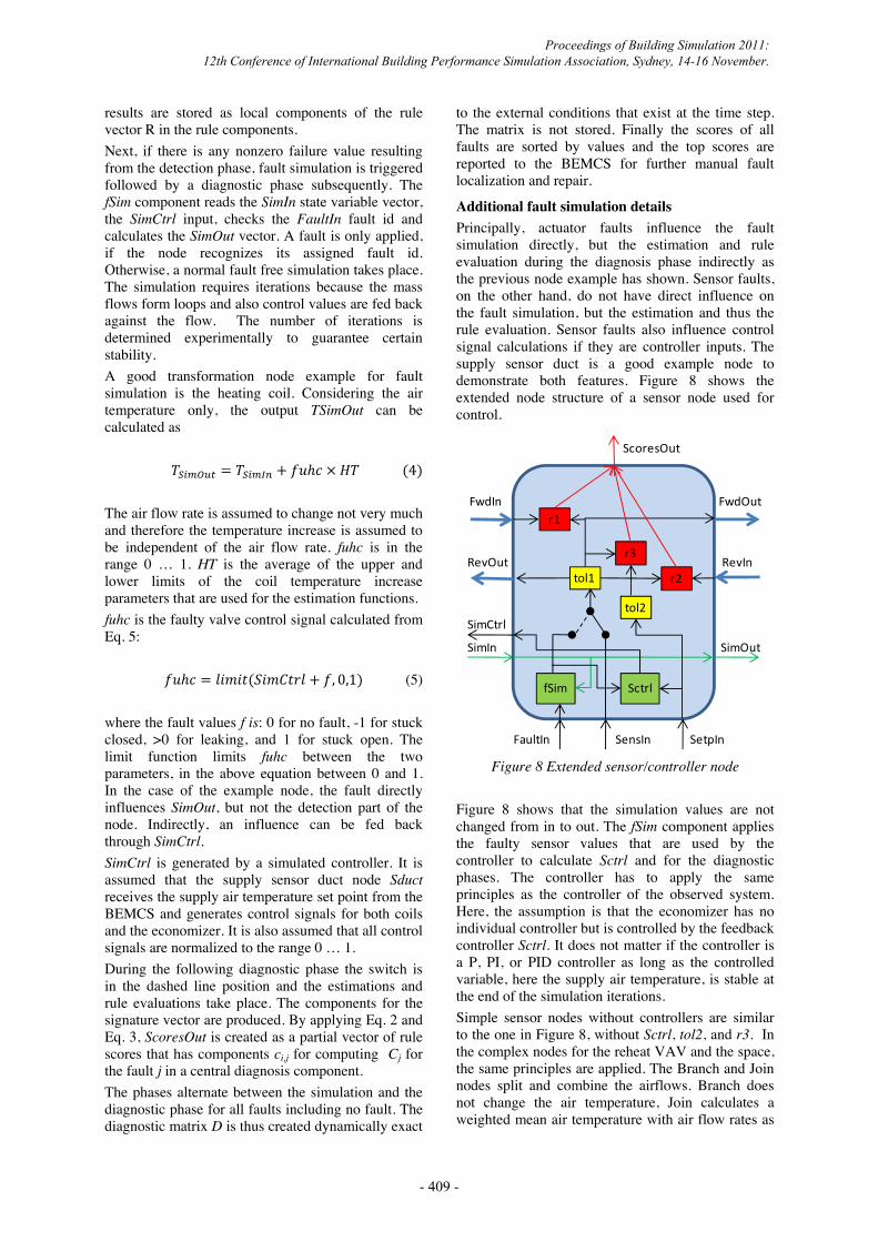
Additional fault simulation details Principally, actuator faults influence the fault simulation directly, but the estimation and rule evaluation during the diagnosis phase indirectly as the previous node example has shown. Sensor faults, on the other hand, do not have direct influence on the fault simulation, but the estimation and thus the rule evaluation. Sensor faults also influence control signal calculations if they are controller inputs. The supply sensor duct is a good example node to demonstrate both features. Figure 8 shows the extended node structure of a sensor node used for control.

Figure 8 Extended sensor/controller node

Figure 8 shows that the simulation values are not changed from in to out. The fSim component applies the faulty sensor values that are used by the controller to calculate Sctrl and for the diagnostic phases. The controller has to apply the same principles as the controller of the observed system. Here, the assumption is that the economizer has no individual controller but is controlled by the feedback controller Sctrl. It does not matter if the controller is a P, PI, or PID controller as long as the controlled variable, here the supply air temperature, is stable at the end of the simulation iterations. Simple sensor nodes without controllers are similar to the one in Figure 8, without Sctrl, tol2, and r3. In the complex nodes for the reheat VAV and the space, the same principles are applied. The Branch and Join nodes split and combine the airflows. Branch does not change the air temperature, Join calculates a weighted mean air temperature with air flow rates as

FwdIn FwdOut

RevInRevOuttol1

r1

r2

r3

ScoresOut

SensIn SetpIn

tol2

fSim

SimCtrl

SimOutSimIn

Sctrl

FaultIn


- 409 -

weights. The rates are calculated in the VAV depending on the supply air pressure, the duct resistance and the VAV damper position. These weights may not be correct because of open doors between the three spaces or open windows, but it is the best assumption we could make for a simplified model.

Fault diagnosis example Figure 9 shows an example for a sensor fault: sensor Tra always shows a temperature that is 5°C too high.

Figure 9 Failure rule and score output example

Figure 9 shows the results of a test run for 5 day or 120 hours with a time resolution of 1 hour. The outdoor temperature and occupancy patterns will be explained in Chapter Results. Here, the four AHU controller modes are shown in the bottom diagram. The nearly perfect match between the two curves shows that the fault simulation generated control and the control values from the normal operation obtained using the Matlab/Simulink generator, are very close. The first diagram from the top shows failure values of three selected rules in the AHU that reach the highest values during the 5 days. There is a time period between Hour 56 and 85 when only one rule shows non zero values. This rule detects the fault at all times. The second diagram shows the simulated failure values for the same rules during the diagnostic phase for the fault that matches the fault in the input data. The rule outputs for all other faults of the list are

generated as well, but not shown here. The diagram is in most parts very similar to the first diagram; only in the time period between 56 and 85 it shows more failures. The third diagram shows the products of three failure values from the two top diagrams. The products promise a high total score for this fault, but do not guarantee it. At least the high score gives a hint where to look for a fault during maintenance.

RESULTS For testing purpose, artificial outdoor air temperature and occupancy pattern time sequences are generated with a time resolution of 0.1h. The total time duration is 5 days with temperatures ranging from -14 to 40°C and a daily sinusoidal variation between 4 am and 4 pm of 14°C. Occupancy is regular between 7 am and 6 pm in all three spaces. The supply air temperature set-point is a function of the outdoor air temperature. Space temperature set-point ranges are (20, 22°C) during occupancy and (17, 25°C) otherwise. Occupancy also determines the heat load in the spaces. Figure 10 shows the outdoor temperature and occupancy of the data files.

Figure 10 Test data outdoor temperature and occupancy

Additional parameters are assumed, for example, space heat gains and losses. A Simulink model has been set up with interactive fault settings to generate data files with fault simulation. The AHU controller model has three PI controllers to generate control signals for the economizer damper and the two coils. All three controllers share the supply air temperature and its set-point as inputs. The controller switches between four modes: heating, swing, cooling with full and with minimal outdoor air. Each of the three VAV controllers has two PI controllers for the damper and the reheat coil. Inputs are the space temperature, the set-point range, and the occupancy. The controller switches between heating and cooling mode. The modes are important for FDD because they determine the observability of faults, especially actuator faults. For example, in the heating mode, the

0 24 48 72 96 120-0.5

0

0.5

1detection phase rule values

0 24 48 72 96 120-1

0

1

2corresponding diagnostic phase rule values

0 24 48 72 96 1200

0.5

1corresponding total scores

0 24 48 72 96 120

1

2

3

4

AHU controller modes

time/hour

-0.2

0

0.2

0.4

0.6

0.8

1

1.2

-20

-10

0

10

20

30

40

50

0 24 48 72 96 120

occupan

cy

Toa/°C

time/h

Toa

occ


- 410 -

outdoor air damper of the mixing box is set at minimum position. The cooling coil valve is closed. Accordingly, stuck closed faults cannot be detected in either node during the heating mode. Therefore, the results have to be interpreted in relation to the modes.

Figure 11 total score result for Tra sensor +5°C

fault

Figure 11 shows the measured total scores for the fault example (Tra +5°C) in Figure 9. Figure 11 shows that the causing fault does not always have the highest rank. The mixing box return air (ra) damper stuck 0 fault reaches the highest total score for low outdoor temperatures (Hours 0 to 55), the outdoor air (oa) damper stuck 1 fault reaches the next highest total score for nearly the same period. This can be understood because both faults have similar effects as the return air +5°C fault. For high outdoor temperatures (Hours 55 to 120) the causing return air temperature sensor fault has the highest total score, followed by the Tma -5 fault. This example shows how difficult fault diagnosis is in detecting the causing fault uniquely. Therefore, it is more realistic to sort the scores and apply ranks from the highest score as rank 1 down and to test, how often the causing fault is one of the top three ranks, as shown in Table 1. Looking at the fifth column of the table, there are several cases with 80 or more % of the time being diagnosed as one of the top three ranks. Some cases such as oad stuck 0 can partly be explained with the modes: in modes 1 and 4 the outdoor air damper is closed anyway and the fault cannot be detected. The same explanation can be applied to the heating and cooling coil valve stuck closed cases because they are also closed during several modes. More problematic are Toa faults. In these cases the generic solution does not work because the result of the outdoor air sensor is one of the external conditions and the fault simulation does not work correctly in this case.

Table 1 Total score ranking results for the AHU faults

rank 1 2 3 1 to 3 fault % Tra sens +5 56 13 29 98 Tra sens -5 69 26 2 97 Toa sens +5 0 0 0 0 Toa sens -5 0 0 2 2 oad stuck 0 6 4 12 22 oad stuck 1 1 51 4 56 oad leak 0 0 6 6 rad stuck 0 72 4 4 80 rad stuck 1 2 7 1 10 rad leak 0 0 0 0 Tma sens +5 76 13 11 100 Tma sens -5 55 36 9 100 hcv stuck 0 9 2 0 11 hcv leak 0.2 0 7 40 47 cv stuck 0 51 1 0 52 cv leak 0.2 34 17 5 56 Tsa sens +5 73 18 1 92 Tsa sens -5 82 2 1 85

Offline tools have been developed to analyze the reasons why the diagnosis does not show better results in some cases. Figures 9 and 10are sample outputs. The HFM-FDD java implementation has several reporting features to provide the necessary data. This is planned as future work, in addition to testing HFM-FDD with different HVAC systems, real or simulated. Future simulations will be based on HVACSim+ models to get more realistic fault simulation data inputs. Li’s work (Li 2010) will be used for this purpose. It is also expected that more detailed BIMs of HVAC systems and related spaces will become available. There are several potential ways to improve the results. Special rules can be introduced; normalization factors can be tuned; fault simulation parameters can be adjusted and so forth. We are currently looking for solutions for such improvements that are generic, can be automated, and do not increase the engineering effort. Such solution will also require additional information about the analyzed HVAC system, defined in the appropriate BIM notation.

CONCLUSION In this paper we report our latest research on extending the Heat Flow Model (HFM) with distributed fault simulation functions and using an associative network for fault diagnosis to map the

0 24 48 72 96 1200

0.25

0.5

0.75

1

1.25

1.5

1.75

2

time/h

tota

l sco

re

Tra +5°C oa damper stuck 1ra Tma -5°C ra damper stuck 0


- 411 -

reported failures back to the most probable faults. The main contribution is the automatic generation of the associative network at run-time and for the current external conditions. This has been achieved by extending the HFM nodes by fault simulation functionality. The diagnosis results are not yet satisfying and will be improved, for example by better similarity metrics. This is ongoing research. A software prototype implementation of the proposed FDD, based on extended HFM, has been performed and tested with a Matlab/Simulink simulated HVAC control system. The implementation uses the java Reflection model to translate the building model based HFM automatically into an executable java program for fault detection and diagnosis, based on a generic java class library for the HFM components. The simulation results demonstrate the effectiveness of our approach. Currently, a test with a real and complex HVAC system with two AHUs and 130 temperature controlled spaces has been started. In addition to the air flow circuit, hot and chilled water supplies will be modelled. 5850 data points can be accessed via BACnet. Due to the generic nature of the FDD-HFM such experiments can be conducted with relatively low effort, based on the automatic generation capabilities of java and the provided node library. Therefore, we mainly use the current implementation as engine to learn from experiments and further develop and improve the field of FDD for HVAC systems. Nevertheless, the implementation can also be used as an application directly or can be treated as specification for an implementation in a different computer language if required.

REFERENCES Baer, K., M. Hinkelmann, M. Schöckle, 1996.

Associative Networks. In Building Optimization and Fault Diagnosis Source Book, IEA Annex 25, p.219-222

Katipamula, S. and M.R. Brambley, 2005a. Methods for fault detection, diagnostics and prognostics for building systems- A review, Part I. IJHVAC&R Research, vol.11 (1):3-25.

Katipamula, S. and M.R. Brambley, 2005b. Methods for fault detection, diagnostics and prognostics for building systems- A review, Part II. IJHVAC&R Research, vol.12 (2):169-187.

Li, S. 2010. A Model-Based Fault Detection and Diagnostics Methodology for Secondary HVAC Systems, PhD Thesis, Drexel University, Philadelphia, USA

Lu, Y., G. Zimmermann, and G. Lo. 2010. Fault Detection and Diagnosis of HVAC Systems Based on a New Heat Flow Model (HFM). Proceedings IAQVEC 2010, The 7th International Conference on Indoor Air Quality,

Ventilation, and Energy Conservation in Buildings, Syracuse, USA

Zimmermann, G., Y. Lu, and G. Lo. 2010. Heat flow modeling of HVAC systems for fault detection and diagnosis. Proceedings SimBuild 2010, Fourth National Conference of IBPSA-USA, New York, p. 215-222.

Lu, Y., G. Zimmermann, and G. Lo. 2010. Fault Detection and Diagnosis of HVAC Systems Based on a New Heat Flow Model (HFM). Proceedings IAQVEC 2010, The 7th International Conference on Indoor Air Quality, Ventilation, and Energy Conservation in Buildings, Syracuse, USA


- 412 -

a simulation based fault diagnosis strategy using … · the hfm fault detection method works in...

Documents