1

A SIMPLIFIED METHOD FOR DYMANIC RESPONSE ANALYSIS OF SOIL-PILE-BUILDING INTERACTION SYSTEM IN LARGE STRAIN LEVELS OF

SOILS

Shin’ichiro TAMORI Shinshu University, Nagano, Japan, snowman@gipwc.shinshu-u.ac.jp

Masanori IIBA Building Research Institute, Min. of Land, Infrastructure and Transport, Tsukuba, Japan

Yoshikazu KITAGAWA Keio University, Yokohama, Japan

ABSTRUCT

A series of shaking-table tests of a scaled soil-pile-building model were performed in order to study the effects of the plastic deformation of soil on dynamic characteristics of the soil-pile-building interaction system. The elasto-plastic material for model ground was made by Plasticine, whose strain dependency of the stiffness and the damping are similar to those of clayey soils. The input motion is 1968 Hachinohe EW and its maximum accelerations were set to be 100, 300 600 cm/s2 at the shaking table. Results show the average value of maximum soil strain became from 0.0018 to 0.018 and the natural frequency and the amplification factor decrease by 28% and 39%, respectively. Dynamic response analyses, which combined the mass-spring model (SR model) having swaying and rocking spring and dashpots located at the foundation of the building and an equivalent linearization method, were carried out. The difference in the natural frequency obtained by the test and analyses were within 5% and those of maximum acceleration at the building are within 10%. KEYWORDS: Soil-pile interaction, Sway-Rocking model, soil non-linearity, equivalent linearization method

1. INTRODUCTION

When designing a building, it is important to evaluate earthquake performance of a building including non-linear soil-building interaction effects during an earthquake. FEM models or Penzien’s models are efficient to do dynamic response analyses for a soil-pile-building interaction system including non-linear soil effects. For FEM models, large calculation time and high computational performance is needed and for Penzien’s models, there are uncertainties in evaluating of virtual mass around the piles or ground springs. So, those methods are not common in practical designing processes. In the practical designing of a building, analytical methods should be simple so that, for example, an equivalent linearization method, like SHAKE, have been used frequently to calculate ground responses. But, in the case of the non-linear soil-building interaction system, the accuracy of the method had not been tested enough. There were several researches using the thin layer element method for having reduced the rigidity of ground around the foundation or piles. That method was applied for analyses of calculating dynamic impedance of a foundation (Miura 1995), or vibration tests of piles (Kusakabe 1994). In the case of vibration tests analysis, an equivalent method was employed, but that was not applied for earthquake response analyses. In this study, a series of shaking table tests were done in order to evaluate the effect of plastic deformation of soils on dynamic characteristics of soil-pile-building interaction system. Dynamic response analyses, which combined Sway-Rocking model and an equivalent linearization method, of the tests were done. Static FEM analyses were also done to estimate effects of soil’s non-linearity around piles, and these results were used in the dynamic analyses.

2. PLASTIC MATERIAL FOR GROUND MODEL Plastic material for the artificial ground model used in this study was made of Plasticine and oil. Plasticine,

2

being a mixture of calcium-carbonate and oil, has been used as a model material for plastic deformation processing of steel, since it has restoring force curves similar to high- temperature steel. Fig. 1 shows the soil characteristics, strain-shear modulus and strain-damping factor relationships for actual clayey soils and Plasticine, which is the plastic soil material used in this shaking table tests. The initial shear modulus, Gt (strain being 1.0 x 10-5), shear modulus at large strain levels, Gs, and damping factors, hg, were obtained by tri-axial compression tests in which ambient stress were kept at 1.0 kg/cm2 and exciting frequency was 1.0Hz. The shear modulus and damping factor of the plastic soil material, Plasticine, has strain dependency similar to those of actual clayey soils.

3. OUTLINE OF SHAKING TABLE TESTS The similarity that proposed by Buckingham was used in modeling the building and the ground soils. The scale factors calculated from this formula are summarized in Table 1. This similarity is applicable to non-linear soil dynamics when the soil model material has a shear modulus-strain and a damping factor-strain relation similar to that of the prototype (Kagawa 1987). Under these conditions the ratio of shear forces in the model and the prototype were kept approximately equal to that of the damping forces for wide strain levels of soil. Fig. 2 shows an outline of the building and the ground model together with the location of the measurement apparatus. Two dwelling units of 11-story buildings were modeled in the transverse direction. Table 2 shows the natural frequency and damping factor of the building model. The building model was made of steel weight and its columns were made of steel plates. The building foundation was made of aluminum and acryl plates. Four pillar-shaped(φ38mm, length is 487mm) pile models were made of steel plate attached with rubber, they were set at the corners of the foundation. The ground model has a block shape and its size is 2x1.46x0.6m. Stainless plates were set at both side ends in transverse direction of the ground to prevent vertical motion of the ground. The central part(φ800mm, depth is 387mm) of the ground model was made from Plasticine and oil. The remaining portions of the model were composed of polyacrylamid and bentnite, and remained elastic throughout the tests. Table 3 shows characteristics of the ground. Damping factors were obtained by a free torsional vibration test and shear wave velocity was obtained by the P-S wave propagation tests. An earthquake records in which the time length was corrected according to the similarity were used for the input ground motion: 1968 Hachinohe EW. Its maximum accelerations were set as 100, 300 and 600 cm/s2 on the shaking table.

4. RESULTS OF THE TESTS Fig. 3 shows the first natural frequencies derived by spectral ratios (BH6/SH5), and average value of maximum soil shear strains. The average value of maximum shear strains shown in Fig. 3 and 4 are calculated as follows: (1) The displacement at SH5, SH4, SH3 and SH2 was calculated after the acceleration records at four points were integrated twice. (2) Maximum relative displacements divided by those distances, and they become maximum strains. (3) The average value of maximum shear strains were average value of the maximum strains between SH5 and SH4, SH4 and SH3, and SH3 and SH2. Fig. 3 shows the average values of maximum strains were about from 0.0018 to 0.018, and the first natural frequencies were from 8.25Hz to 6.0Hz. Fig. 4 shows the amplification factors, those are amplitude of the spectral ratios (BH6/SH5) at the natural frequency, and the average value of maximum strains. The amplification factors are about from 7.1 to 4.3. So, the natural frequency and the amplification factors, when the maximum input motions acceleration was 600 cm/s2, become 72% and 61% of those when it was 300cm/s2.

5. THEORETICAL MODEL 5.1 Outline The theoretical model employed in this study was the Sway-Rocking (SR) model, and an equivalent linearization method was used for non-linear analyses. Dynamic stiffness of the pile foundation were calculated as follows:

3

(a) Dynamic stiffness of piles for horizontal and rocking motion proposed by Novak and Nogami (Novak and Nogami 1977) were employed. Group effects factor, which was 0.72 in this case, were derived by Iiba’s method (Inoue et. al. 1988). (b) Dynamic stiffness of piles for vertical motion was calculated by Novak’s method (Novak 1977). 5.2 Soil Ground Shear modulus, Gs, and damping factor, hg, of the soil were determined by the tri-axial compression tests according to the following equation modified by the Hardin-Drnevich model (Hardin and Drnevich 1972):

(1)

(2)

Where Gt is the initial shear modulus and γs is shear strain of the soil. 5.3 Soil Non-Linearity around Pile Effects on soil non-linearity around piles were evaluated by a static FEM analysis. Fig.5 shows a FEM model, which was1/2 symmetry model, for the static analysis, and its radius was 50cm, depth was 51cm and pile length was 47cm. The lower layer of the ground layer was elastic media and the upper layer elasto-plastic media, which follow the Drucker-Prager’s yield function. Its cohesion was 0.02kgf/cm2 and angle for internal friction was 0°. Boundary conditions for the analyses are follows: (a) Botton and circumference part of the ground was fix. (b) Pile cap had freedom degree in only horizontal direction, so pile cap’s rotation was inhibited. (c) Horizontal force was applied at the pile cap. Fig. 6 shows horizontal stiffness coefficient obtained by the static FEM analysis. kh0 is initial horizontal coefficient of subsoil reaction and khs are those at some strain. khs was calculated by equation (3).

(3)

where, P: applied force, EI: bending stiffness of pile, D: pile diameter, y: pile displacement Fig.7 is also results of the same static FEM analyses in the case for the prototype. In Fig.7, the well-known relation of kh and displacement are also plotted. Those two curves are very close when displacements are from 0.5 cm to 4cm. From the results of the static FEM analyses, we got following relation.

(4)

where kh0:initial horizontal coefficient of subsoil reaction, khs: horizontal coefficient of subsoil reaction when pile cap displacement isδp 5.4 Estimation of soil’s strain Effects on soil non-linearity were evaluated according to soil’s strain. In case of earthquake response of soil-building interaction system, we have to consider soil strain by free filed motion of the ground, γwave in equation (5), and that by foundation displacement, γP in equation (5). In this study, former are measured value, which is the average value of maximum shear strain, shown in Figs. 3 and 4. Later were evaluated as follows: (a) we made response analyses of SR model at initial condition and got maximum relative displacement of pile foundation. (b) we calculated kh0/khs factor by equation (4) from maximum relative displacement. (c) khs should be proportion to shear stuffiness of soil, Gs, so we put kh0/khs into the left term of equation (1), and calculated

sγ . (d) Equivalent strain of soil, γeq ,was calculated by equation (5).

(5)

258.1)002072.0/(96.0101.1

st

s

rGG

+=

)/1(145.0035.0 tsg GGh −+=

yEI

DkEIP hs

3

44

4 ���

����

�=

03741.0)05108.0/(1

03741.014856.1

0

++

−=ph

hs

kk

δ

22pwaveeq γγαγ +=

4

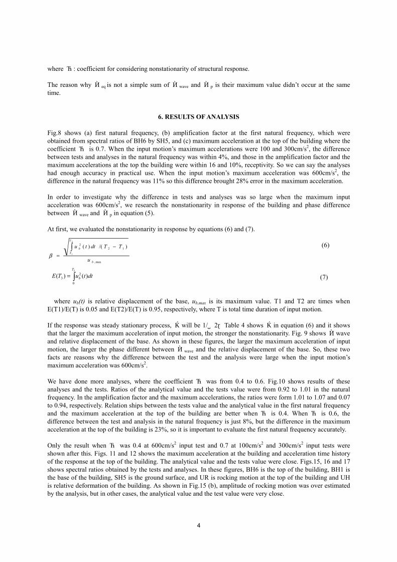
where α: coefficient for considering nonstationarity of structural response. The reason why γeq is not a simple sum of γwave and γp is their maximum value didn’t occur at the same time.

6. RESULTS OF ANALYSIS Fig.8 shows (a) first natural frequency, (b) amplification factor at the first natural frequency, which were obtained from spectral ratios of BH6 by SH5, and (c) maximum acceleration at the top of the building where the coefficient α is 0.7. When the input motion’s maximum accelerations were 100 and 300cm/s2, the difference between tests and analyses in the natural frequency was within 4%, and those in the amplification factor and the maximum accelerations at the top the building were within 16 and 10%, receptivity. So we can say the analyses had enough accuracy in practical use. When the input motion’s maximum acceleration was 600cm/s2, the difference in the natural frequency was 11% so this difference brought 28% error in the maximum acceleration. In order to investigate why the difference in tests and analyses was so large when the maximum input acceleration was 600cm/s2, we research the nonstationarity in response of the building and phase difference between γwave and γp in equation (5). At first, we evaluated the nonstationarity in response by equations (6) and (7).

(6)

(7)

where ub(t) is relative displacement of the base, ub,max is its maximum value. T1 and T2 are times when E(T1)/E(T) is 0.05 and E(T2)/E(T) is 0.95, respectively, where T is total time duration of input motion. If the response was steady stationary process, βwill be 1/√2．Table 4 shows βin equation (6) and it shows that the larger the maximum acceleration of input motion, the stronger the nonstationarity. Fig. 9 shows γwave and relative displacement of the base. As shown in these figures, the larger the maximum acceleration of input motion, the larger the phase different between γwave and the relative displacement of the base. So, these two facts are reasons why the difference between the test and the analysis were large when the input motion’s maximum acceleration was 600cm/s2. We have done more analyses, where the coefficient α was from 0.4 to 0.6. Fig.10 shows results of these analyses and the tests. Ratios of the analytical value and the tests value were from 0.92 to 1.01 in the natural frequency. In the amplification factor and the maximum accelerations, the ratios were form 1.01 to 1.07 and 0.07 to 0.94, respectively. Relation ships between the tests value and the analytical value in the first natural frequency and the maximum acceleration at the top of the building are better when α is 0.4. When α is 0.6, the difference between the test and analysis in the natural frequency is just 8%, but the difference in the maximum acceleration at the top of the building is 23%, so it is important to evaluate the first natural frequency accurately. Only the result when α was 0.4 at 600cm/s2 input test and 0.7 at 100cm/s2 and 300cm/s2 input tests were shown after this. Figs. 11 and 12 shows the maximum acceleration at the building and acceleration time history of the response at the top of the building. The analytical value and the tests value were close. Figs.15, 16 and 17 shows spectral ratios obtained by the tests and analyses. In these figures, BH6 is the top of the building, BH1 is the base of the building, SH5 is the ground surface, and UR is rocking motion at the top of the building and UH is relative deformation of the building. As shown in Fig.15 (b), amplitude of rocking motion was over estimated by the analysis, but in other cases, the analytical value and the test value were very close.

�=3

0

23 )()(

T

b dttuTE

max,

122

2

1

)/()(

b

T

Tb

u

TTdttu� −

=β

5

CONCLUTION We proposed a simplified method for dynamic response analyses, which consisted of Sway-Rocking model and an equivalent linearization method. The accuracy of the method was examined by shaking table tests of elasto-plastic soil-pile-building interaction system. Results of the analyses were as follows: (1) The average value of the maximum strain of soil ground became 0.0018 to 0.018, according to those

changing of the soil condition, the natural frequency of the soil-pile-building system became from 8.25Hz to 6.0Hz and the amplification factor became from 7.1 to 4.3.

(2) Ratios of the tests value and analytical value in the natural frequency, the amplification factor and the maximum acceleration at the top of the building were from 0.99 to 1.04, 0.84 to 1.09 and 0.94 to 1.10, respectively, so, the proposed method had enough accuracy for practical use in designing buildings. But, when the maximum input acceleration was 600cm/s2, the coefficients that considered nonstationarity of the soil and the building response should be smaller than those when the maximum input acceleration was 100 and 300 cm/s2. We pointed the reason why the coefficient should be changed were (a) the lager the amplitude of input motion, the lager the level of nonstationarity in relative displacement of the pile foundation, and (b) the lager the phase difference between strain by the free field motion and that by the pile foundation’s displacement.

REFERENCE Hardin, B. O. and Drnevich, V. P.(1972). “Shear modulus and damping in soils, Design equation and curves”,

Journal of Soil Mech. and Foundation, Div. ASCE, 98(SM7), 667-692. Inoue, Y., Osawa, Y., Matushima, Y, Kitagawa, Y., Yamazaki, Y. and Kawamura, S. (1988).“A Proposal for

Seismic Design Procedure of Apartment Houses Including Soil-Structure Interaction Effect ”, Proc. of Ninth World Conference on Earthquake Engineering, Vol. 8, 365-370.

Kagawa, T. (1987). “On the similitude in model vibration tests on earthquakes.”, Proc. of Japan Society of Civil Engineering, 275, 69-77

Kusakabe, K., Yasuda, T. and Maeda, Y. (1994). “Dynamic Characteristics of Soil-Pile Foundation System in Non-Linear Soil Medium”, Proceedings of The Ninth Japan Earthquake Engineering Symposium, Vol.2, 1219-1224.

Miura, K., Masuda, K., Maeda, T. and Kobori, T. (1995),“Nonlinear Dynamic Impedance of Pile Group Foundation”, Proc. 3rd Int. Conf. On Recent Advances in Geotechnical Earthquake Eng. and Soil Dynamics, 417-422.

Novak, M. and Nogami, T. (1977),“Soil-Pile Interaction in Horizontal Vibration, Earthquake Engineering and Structural Dynamics”, Vol.5, 263-281.

Novak, M. (1977),“Vertical Vibration of Floating Piles”, Proceedings of the American Society of Civil Engineers, Vol.103, EM1, 153-168.

6

Table 1: Similitude Ratios Item Ratio (Model/Prototype)

Soil Density

Length

Acceleration

kgf/cm3

cm

cm/s2

１／η

１／λ

１

1

1/40

1

Displacement

Mass

Shear Modulus

Frequency

Velocity

Stress

Strain

cm

kgf.s2/cm

kgf/cm2

1/s

cm/s

kgf/cm2

１／λ

１／ηλ３

１／ηλ

√λ

１／√λ

１／ηλ

１

1/40

1/6.4×104

1/40

6.325

1/6.325

1/40

1

Table 2: Characteristics of Building Model

Foundation Building Characteristics of Fixed Base

Building Size (cm)

Weight (kgf)

Height (cm)

Weight (kgf)

Natural Freq. (Hz)

DampingFactor

(%)

30 × 30

6.79

78.7

28.4

18.8

0.22

Table 3: Characteristics of Ground Model Upper Layer

(GL～GL-45cm) Item Center Edge

Lower Layer (GL-45～60cm)

Vs(m/s) Damping Factor(%)

Density(gf/cm3)

23.7 6.63*1.57

18.4 5.57 1.17

36.0 6.05 1.41

*Strain level is 3.6×10-4

0

5

10

15

20

25

30

1.E-06 1.E-04 1.E-02

Shear Strain

Dam

ping

fac

tor

(%)

PLASTICINESeed-IdrissIshiharaHara

0

0.2

0.4

0.6

0.8

1

1.2

1.E-06 1.E-04 1.E-02Shear Strain

Gs/

Gt

PLASTICINESeed-IdrissIshiharaNishigakiHaraTaylor-PartonAndersonA d 2

Fig. 1 Soil Characteristics

Table 4: Nonstationarity in relative displacement of foundation

Maximum input

acc. (cm/s2) β in equation (6)

100 0.378

300 0.267

600 0.216

7

Fig.3 First natural frequency andaverage value of maximum soil

strain

Fig.4 Amplification factor andaverage value of maximum soil

strain

Fig.5 FEM model forstatic analysis

Fig. 2 Test model

0

0.2

0.4

0.6

0.8

1

1.2

0.001 0.01 0.1 1 10

displacement(cm)

khs/

kh0

Fig. 6 Horizontal coefficient of subsoil reactionand pile displacement

0.1

1

10

0.1 1 10

displacement(cm)

khs/

kh(δ

=1.0

)

khs/kh(δ=1.0)

khs=kh(δ=1.0)*δ^(-0.5)

Fig. 7 Horizontal coefficient of subsoil reaction andpile displacement

(displacement’s scale is for prototype)

(a) Section (b) Plan

0

2

4

6

8

10

0.001 0.01 0.1

average value ofmaximum strain

natu

ral fr

eque

ncy(

Hz)

0

1

2

3

4

5

6

7

8

0.001 0.01 0.1

average value ofmaximun strain

ampl

ific

atio

n fa

ctor

8

0

2

4

6

8

10

0 2 4 6 8 10

tests(a) natural frequency(Hz)

anal

yses

100cm/s/s

300cm/s/s600cm/s/s

0

2

4

6

8

10

0 2 4 6 8

tests(b)amplification factor

anal

yses

0

2500

5000

0 2500 5000

tests(c) maximum acc. (cm/s/s)

anal

yses

5

5.5

6

6.5

5 5.5 6 6.5

tests(a) natural frequency(Hz)

anal

yses

α=0.6

α=0.5

α=0.4

4

4.2

4.4

4.6

4.8

5

4 4.2 4.4 4.6 4.8 5

tests(b)amplification factor

anal

yses

3000

4000

5000

3000 4000 5000tests

(c) maximum acc. (cm/s/s)

anal

yses

-1.5

-1.0

-0.5

0.0

0.5

1.0

1.5

1.8 2.0 2.2 2.4 2.6 2.8 3.0 3.2

sec(c) 600cm/s/s

-1.5

-1.0

-0.5

0.0

0.5

1.0

1.5

1.8 2.0 2.2 2.4 2.6 2.8 3.0 3.2

sec(b) 300cm/s/s

-1.5

-1.0

-0.5

0.0

0.5

1.0

1.5

1.8 2.0 2.2 2.4 2.6 2.8 3.0 3.2sec

(a) 100cm/s/s

relative displacement

wave

0

20

40

60

80

100

120

140

0 500 1000 1500

maximum acc.(cm/s/s)(a) 100cm/s/s

pos

itio

n(cm

)

test

analysis

0

20

40

60

80

100

120

140

0 2000 4000

maximum acc.(cm/s/s)(b) 300cm/s/s

pos

itio

n(cm

)

0

20

40

60

80

100

120

140

0 2500 5000

maximum acc.(cm/s/s)(c) 600cm/s/s

pos

itio

n(cm

)

-1000

-500

0

500

1000

1.5 2.5 3.5 4.5 5.5 6.5

sec(a) test

cm

/s/

s

-1000

-500

0

500

1000

1.5 2.5 3.5 4.5 5.5 6.5

sec(b) analysis

cm

/s/

s

Fig. 8 Results of tests andanalyses (α =0.7)

Fig. 9 Relative displacement of base and stain ofground by wave propagation

Fig. 10 Results of testsand analyses (600cm/s/s)

Fig. 11 Maximum acceleration’s distribution

Fig. 12 Acceleration at the building (100cm/s/s)

9

-3000-2000-1000

0100020003000

1.5 2.5 3.5 4.5 5.5 6.5

sec(a) test

cm

/s/

s

-3000-2000-1000

0100020003000

1.5 2.5 3.5 4.5 5.5 6.5

sec(b) analysis

cm

/s/

s

-5000

-2500

0

2500

5000

1.5 2.5 3.5 4.5 5.5 6.5

sec(a) test

cm

/s/

s

-5000

-2500

0

2500

5000

1.5 2.5 3.5 4.5 5.5 6.5

sec(b) analysis

cm

/s/

s

0

1

2

3

4

5

6

0 10 20 30Hz(a) BH6/SH5

testanalysis

0

1

2

3

4

5

6

0 10 20 30Hz

(b) UR/SH5

0

0.5

1

1.5

2

2.5

3

0 10 20 30Hz

(c) BH1/SH5

0

1

2

3

4

5

6

7

8

0 10 20 30Hz(a) BH6/SH5

test

analysis

0

0.5

1

1.5

2

2.5

3

3.5

4

0 10 20 30Hz(b) UR/SH5

0

0.5

1

1.5

2

2.5

3

3.5

0 10 20 30Hz

(c) BH1/SH5

0

1

2

3

4

5

6

7

8

9

0 10 20 30Hz(a) BH6/SH5

testanalysis

0

1

2

3

4

5

6

0 10 20 30Hz

(b)UR/SH5

0

0.5

1

1.5

2

2.5

3

3.5

0 10 20 30Hz

(c)BH1/SH5

Fig. 13 Acceleration at the building (300cm/s/s) Fig. 14 Acceleration at the building (600cm/s/s)

Fig. 15 Spectral ratios (100cm/s/s) Fig. 16 Spectral ratios (300cm/s/s) Fig. 17 Spectral ratios (600cm/s/s)