a simple protocol using underwater epoxy to install annual

United States Department of Agriculture / Forest ServiceRocky Mountain Research StationGeneral Technical Report RMRS-GTR-314October 2013

A Simple Protocol Using Underwater Epoxy to Install Annual Temperature Monitoring Sites in Rivers and Streams

Daniel J. Isaak Dona L. Horan Sherry P. Wollrab

Isaak, Daniel J.; Horan, Dona L.; and Wollrab, Sherry P. 2013. A simple protocol using underwa-ter epoxy to install annual temperature monitoring sites in rivers and streams. Gen. Tech. Rep. RMRS-GTR-314. Fort Collins, CO: U.S. Department of Agriculture, Forest Service, Rocky Mountain Research Station. 21 p.

Abstract

Thermal regimes in rivers and streams are fundamental determinants of biological processes and are often monitored for regulatory compliance. Here, we describe a simple technique for establishing annual monitoring sites that uses underwater epoxy to attach miniature sensors to large rocks and cement bridge supports, which then serve as protective anchors. More than 500 new monitoring sites were established using the technique from 2010 to 2012 in rivers and streams across the Rocky Mountains. Revisits to 179 sites indicate good sensor retention rates, with 88 - 100% of sensors retained after 1 year in low-gradient streams (<3%) and 70 - 78% retained in high-gradient streams (>3%). Establishing annual monitoring sites with underwater epoxy is inexpensive, can be done in a wide range of water temperatures, and improves data collection efficiency because few site visits are required and measurements are recorded throughout the year.

Keywords: stream temperature, monitoring, underwater epoxy, climate change, thermal regime, TMDL, water quality standard, temperature sensor

Authors _____________________________Daniel J. Isaak is a Research Fisheries Scientist with the U.S. Forest Service, Rocky Mountain Research Station, Aquatic Sciences Laboratory in Boise, Idaho. He holds a B.S. degree from South Dakota State University, a M.S. degree from the University of Idaho, and a Ph.D. from the University of Wyoming. His research focuses on understanding the effects of climate change and natural disturbance on stream habitats and fish populations, monitoring and modeling of stream temperature and fish populations, development and application of spatial statistical models for stream networks, and use of digital and social media to connect people, information, and landscapes.

Dona L. Horan is a Fisheries Biologist with the Rocky Mountain Research Station Boise Aquatic Sciences Laboratory in Boise, Idaho. She holds a B.S. degree from the University of Califor-nia, Berkeley, and a M.S. degree from Utah State University.

Sherry P. Wollrab is a Fisheries Biologist with the Rocky Mountain Research Station Boise Aquatic Sciences Laboratory in Boise, Idaho. She holds a B.S. degree from the University of New Hampshire, and a M.S. degree from the University of Idaho.

Acknowledgments ____________________

Support for this project was provided by the Rocky Moun-tain Research Station and Washington Office of Research and Development in the U.S. Forest Service. The final draft of this report was improved by comments from Andrew Todd, Bruce Rieman, Don Essig, Frank McCormick, and Jen Stamp. We thank Art Butts and Andy Hill for their suggestions to use PVC canisters as solar shields. We also thank the PIBO stream monitoring program and many other biologists and hydrolo-gists who have established temperature monitoring sites using the epoxy technique and provided valuable feedback concerning its efficacy. A discussion with Brett Roper during a turkey hunting trip about previous uses of epoxy to anchor steel cables into boulders for fish screw-traps inspired us to think about applications for temperature monitoring.

Cover: Dona Horan provided the images used on the cover. The stream photograph is of Johnson Creek in central Idaho.

Mention of trade names does not imply endorsement by the U.S. Forest Service.

You may order additional copies of this publication by sending your mailing information in label form through one of the following media. Please specify the publication title and number.

Publishing Services Telephone (970) 498-1392

FAX (970) 498-1122

E-mail [email protected]

Web site http://www.fs.fed.us/rmrs

Mailing Address Publications Distribution Rocky Mountain Research Station 240 West Prospect Road Fort Collins, CO 80526

Contents

Introduction .............................................................................................................. 1

Materials and Methods ............................................................................................ 2

Preparation for the Field ............................................................................... 3Sensor Installation ........................................................................................ 4Data Retrieval and Site Maintenance ........................................................... 9

Results From Previous Sensor Installations ........................................................ 9

Discussion ............................................................................................................. 12

Conclusion .................................................................................................. 14

References ............................................................................................................. 15

Appendix A. Materials Needed to Install an Annual Stream Temperature Monitoring Site Using Underwater Epoxy .............................................. 18

Appendix B. Sample Datasheet With Information to Record During Establishment of an Annual Temperature Monitoring Site. .................. 19

Appendix C. Field Reference Guide: 9 Steps for Installing a Temperature Sensor with Epoxy ............................................................. 20

Appendix D. Downloading a TidbiT v2 Temperature Sensor Using a Data Shuttle ............................................................................................... 21

1USDA Forest Service Gen. Tech. Rep. RMRS-GTR-314. 2013

Introduction

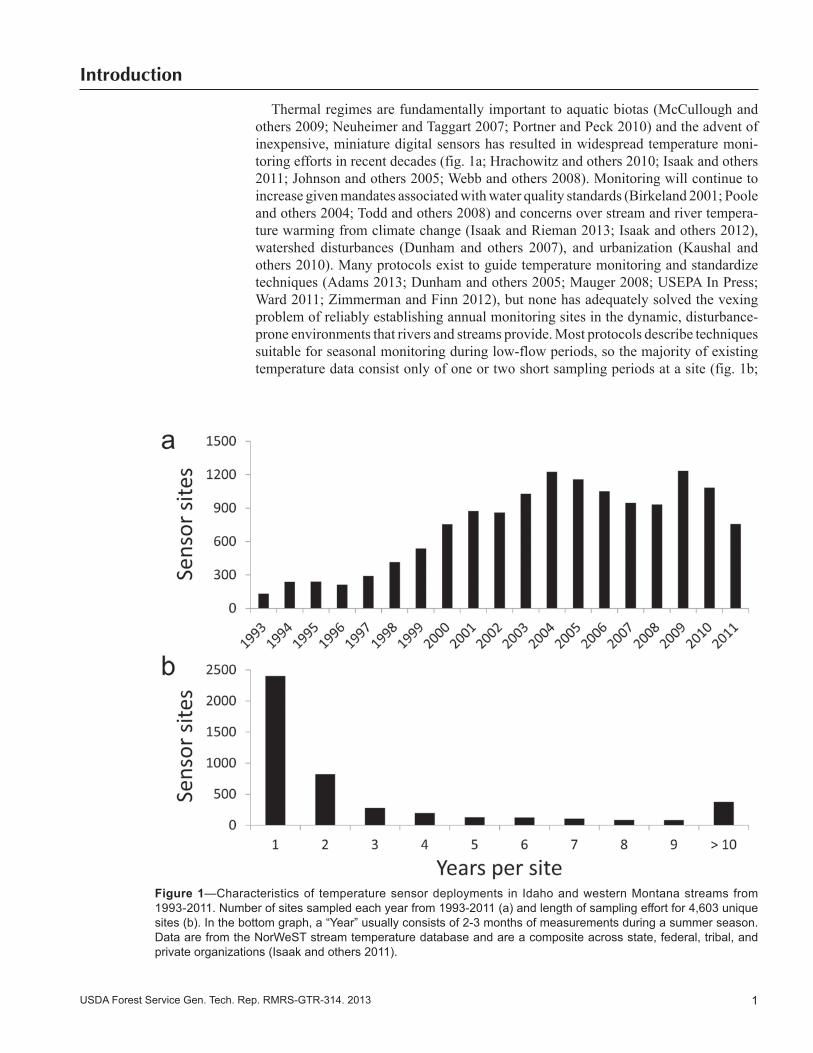
Thermal regimes are fundamentally important to aquatic biotas (McCullough and others 2009; Neuheimer and Taggart 2007; Portner and Peck 2010) and the advent of inexpensive, miniature digital sensors has resulted in widespread temperature moni-toring efforts in recent decades (fig. 1a; Hrachowitz and others 2010; Isaak and others 2011; Johnson and others 2005; Webb and others 2008). Monitoring will continue to increase given mandates associated with water quality standards (Birkeland 2001; Poole and others 2004; Todd and others 2008) and concerns over stream and river tempera-ture warming from climate change (Isaak and Rieman 2013; Isaak and others 2012), watershed disturbances (Dunham and others 2007), and urbanization (Kaushal and others 2010). Many protocols exist to guide temperature monitoring and standardize techniques (Adams 2013; Dunham and others 2005; Mauger 2008; USEPA In Press; Ward 2011; Zimmerman and Finn 2012), but none has adequately solved the vexing problem of reliably establishing annual monitoring sites in the dynamic, disturbance-prone environments that rivers and streams provide. Most protocols describe techniques suitable for seasonal monitoring during low-flow periods, so the majority of existing temperature data consist only of one or two short sampling periods at a site (fig. 1b;

Figure 1—Characteristics of temperature sensor deployments in Idaho and western Montana streams from 1993-2011. Number of sites sampled each year from 1993-2011 (a) and length of sampling effort for 4,603 unique sites (b). In the bottom graph, a “Year” usually consists of 2-3 months of measurements during a summer season. Data are from the NorWeST stream temperature database and are a composite across state, federal, tribal, and private organizations (Isaak and others 2011).

2 USDA Forest Service Gen. Tech. Rep. RMRS-GTR-314. 2013

Isaak and others 2011; Moore 2006; Moore and others 2013). As a result, it is often difficult (or impossible) to describe long-term (i.e., multiple decades) trends in stream temperatures or the full array of characteristics that constitute thermal regimes (e.g., seasonal means and variance, date of spring and winter onset, total annual degree days; Olden and Naiman 2010).

Existing protocols have several additional limitations. First, they are expensive to implement—not with regards to materials, but with regards to the number of site visits that are required for site maintenance. Because existing protocols are usually for sea-sonal monitoring, two site visits are required each year (one for sensor deployment and one for retrieval) and data are collected for a subset of the annual cycle (typically 2 to 3 months). Modern temperature sensors have memory and battery capacities sufficient for continuous measurements over prolonged periods (i.e., 1 to 10 years), so it is inefficient not to use this capacity. Second, existing protocols are obtrusive—often requiring metal bars or other artificial anchor points and steel cables be left in the stream. Third, sensors are often positioned on the streambed, where they are more prone to abrasion or burial by substrates during floods, which results either in sensor loss or biased measurements from interactions with thermally distinct hyporheic waters (Arrigoni and others 2008).

In this report, we describe a simple protocol that uses underwater epoxy to attach sensors to the downstream sides of large rocks and cement bridge supports, which then serve as protective anchors. Earlier research indicated that attachment to these features does not bias temperature measurements and that epoxy installations could withstand large floods (Isaak and Horan 2011). Here, we provide a detailed protocol description that has been refined through hundreds of additional sensor installations. Estimates of sensor retention rates at 1- and 2-year intervals are also provided to facilitate compari-sons with other techniques and to provide users with estimates of the amount of data that a monitoring network will yield.

Materials and Methods

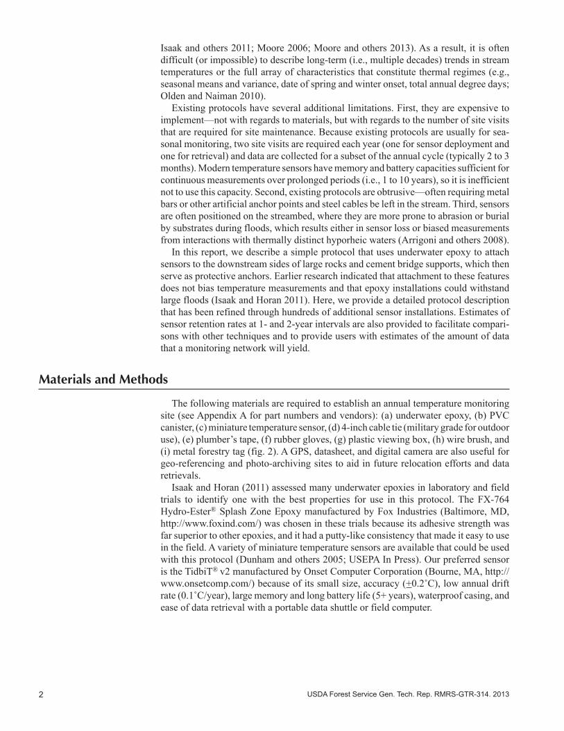
The following materials are required to establish an annual temperature monitoring site (see Appendix A for part numbers and vendors): (a) underwater epoxy, (b) PVC canister, (c) miniature temperature sensor, (d) 4-inch cable tie (military grade for outdoor use), (e) plumber’s tape, (f) rubber gloves, (g) plastic viewing box, (h) wire brush, and (i) metal forestry tag (fig. 2). A GPS, datasheet, and digital camera are also useful for geo-referencing and photo-archiving sites to aid in future relocation efforts and data retrievals.

Isaak and Horan (2011) assessed many underwater epoxies in laboratory and field trials to identify one with the best properties for use in this protocol. The FX-764 Hydro-Ester® Splash Zone Epoxy manufactured by Fox Industries (Baltimore, MD, http://www.foxind.com/) was chosen in these trials because its adhesive strength was far superior to other epoxies, and it had a putty-like consistency that made it easy to use in the field. A variety of miniature temperature sensors are available that could be used with this protocol (Dunham and others 2005; USEPA In Press). Our preferred sensor is the TidbiT® v2 manufactured by Onset Computer Corporation (Bourne, MA, http://www.onsetcomp.com/) because of its small size, accuracy (+0.2˚C), low annual drift rate (0.1˚C/year), large memory and long battery life (5+ years), waterproof casing, and ease of data retrieval with a portable data shuttle or field computer.


Preparation for the Field

Sensor accuracy should be assessed across a range of temperatures and compared to temperature measurements from a more accurate instrument (e.g., a NIST (National Institute of Standards and Technology) certified thermometer) before field deployment. A simple accuracy check can be done by placing multiple sensors in a container, mov-ing the container in and out of a refrigerator for several days, and then examining the data for anomalies. Other protocols provide more details regarding these assessments (Adams 2013; Dunham and others 2005; USEPA In Press). This step will also identify sensors that malfunction during the launch/download sequence or have battery failures. Malfunctioning sensors can be returned to the manufacturer for replacement.

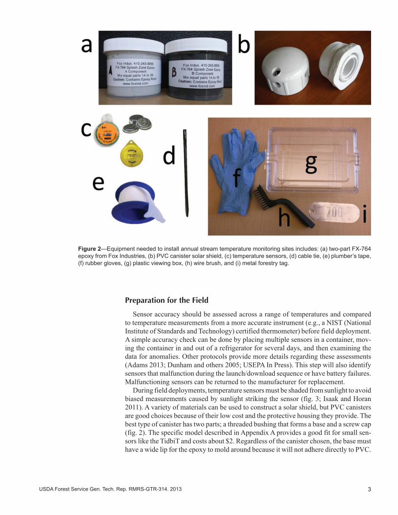
During field deployments, temperature sensors must be shaded from sunlight to avoid biased measurements caused by sunlight striking the sensor (fig. 3; Isaak and Horan 2011). A variety of materials can be used to construct a solar shield, but PVC canisters are good choices because of their low cost and the protective housing they provide. The best type of canister has two parts; a threaded bushing that forms a base and a screw cap (fig. 2). The specific model described in Appendix A provides a good fit for small sen-sors like the TidbiT and costs about $2. Regardless of the canister chosen, the base must have a wide lip for the epoxy to mold around because it will not adhere directly to PVC.

Figure 2—Equipment needed to install annual stream temperature monitoring sites includes: (a) two-part FX-764 epoxy from Fox Industries, (b) PVC canister solar shield, (c) temperature sensors, (d) cable tie, (e) plumber’s tape, (f) rubber gloves, (g) plastic viewing box, (h) wire brush, and (i) metal forestry tag.


To prepare the PVC canister for use as a solar shield, drill several 3/8-inch holes through the sides of the cap to facilitate water circulation. The holes should be placed high on the sides of the cap to avoid overlap with the bushing threads after the cap is screwed to the base. Also drill one hole on the face of the cap near a side hole to pro-vide a location where the sensor can be secured with a cable tie (fig. 4). Plumber’s tape should be wrapped around the threads of the base to ensure easy removal of the cap after extended deployment. If sensors will be placed in streams where human traffic is common, the PVC canister can be painted a neutral color to reduce its visibility.

Sensor Installation

Where sensors are deployed as part of broad-scale sampling designs is beyond the scope of this report, but is covered elsewhere (Dunham and others 2007; Isaak and others 2009; Isaak 2011b; Stevens and Olsen 1999; Zimmerman 2006). Here, we focus only on sensor installations at individual sites. The installation process has nine steps and should be done during low flow periods.

Step 1. Search for a large rock or cement bridge support that has a flat downstream surface that is shielded during floods from moving substrates and debris (fig. 5). Iden-tifying a good attachment site is the most important part of successfully establishing an annual monitoring site, so choose sites carefully. If using a rock as the attachment site, select one that protrudes a foot or more above the low flow water surface to ensure that other rocks will not slide over it and dislodge the sensor during a flood. Do not move rocks into the stream to serve as attachment sites. If you are able to move a rock, it is too small and the next flood will cause the loss of the sensor.

Examine the downstream side of the potential attachment site for pockets of rela-tively calm water. The best sites usually have small substrates like gravels or pebbles that settled out of the main flow as the flood receded. If large rocks and cobbles are on the downstream side of the attachment site, similarly large substrates are likely to

Figure 3—Stream temperature measurements from four sensors at the same site during 8 days in July 2010. All sensors had solar shields during the first 4 days. The solar shield was removed from one sensor on day 5 (black arrow) and temperature spikes became apparent during times when sunlight struck the sensor (repro-duced from Isaak and Horan 2011).


Figure 4—Temperature sensor strapped into the lid of a PVC canister solar shield (a), solar shield assembly with epoxy molded around the base and ready for installation (b), assembly installed on a rock (c), and top removed after installation (d). Holes are drilled through the sides of the shield to make it neutrally buoyant and to facilitate water circulation. Plumber’s tape is wrapped around the threads of the base to ensure easy removal of the cap after extended deployment.

move there again during the next flood and could dislodge the sensor. The site should be sheltered from the main flow path but have well-mixed flows and eddy currents. Water depth must also be sufficient to submerge the sensor during the lowest flows of the year and during extreme drought years.

Step 2. Find a convenient working location near the attachment site to arrange and prepare the materials needed for an installation. If your sensor has an indicator light, check that it is blinking and the sensor is ready to collect data. Record the serial number of the sensor and the metal forestry tag number on the datasheet. Fasten the sensor into the cap of the PVC canister using a cable tie and screw the cap onto the base (fig. 4).


Step 3. Put on rubber gloves and use the wire brush to scrub the attachment surface down to bare rock or cement. Clean an area larger than the PVC canister to provide a variety of microsite locations to choose from when making the final installation. Choose a location that is below the low flow water surface, but several inches above the streambed to minimize the possibility that the sensor will be buried by substrate during subsequent floods. If the sensor does become buried, the temperature recordings may be biased by interactions with hyporheic flows that are thermally distinct from temperatures in the free-flowing stream. We recommend discarding data from sensors that have been entirely buried to avoid this potential bias.

Step 4. Place a flat cobble within easy reach of the attachment site so that it can be leaned against the face of the solar shield canister after installation.

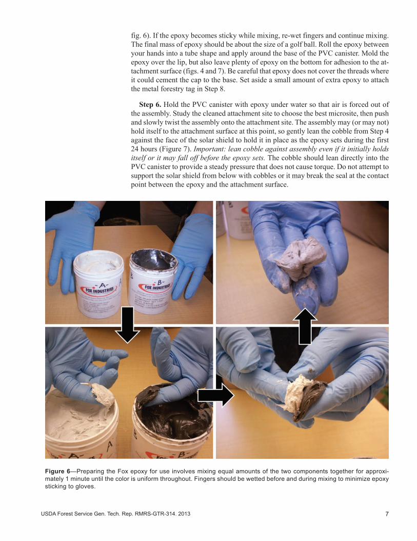
Step 5. Wet gloved fingers in the stream and scoop out equal amounts of white and black epoxy from each container (balls about the diameter of a quarter). Mix epoxy components together until a uniform gray color is achieved (requires at least 1 minute;

Figure 5—Examples of large rocks (a and b) and cement bridge pilings (c and d) that provide good sensor attachment sites. Each site has a flat downstream attachment surface that is shielded during floods from bedload movement and debris. Arrows point to the solar shield containing a sensor; circles highlight metal forestry tags used to monument the site.


fig. 6). If the epoxy becomes sticky while mixing, re-wet fingers and continue mixing. The final mass of epoxy should be about the size of a golf ball. Roll the epoxy between your hands into a tube shape and apply around the base of the PVC canister. Mold the epoxy over the lip, but also leave plenty of epoxy on the bottom for adhesion to the at-tachment surface (figs. 4 and 7). Be careful that epoxy does not cover the threads where it could cement the cap to the base. Set aside a small amount of extra epoxy to attach the metal forestry tag in Step 8.

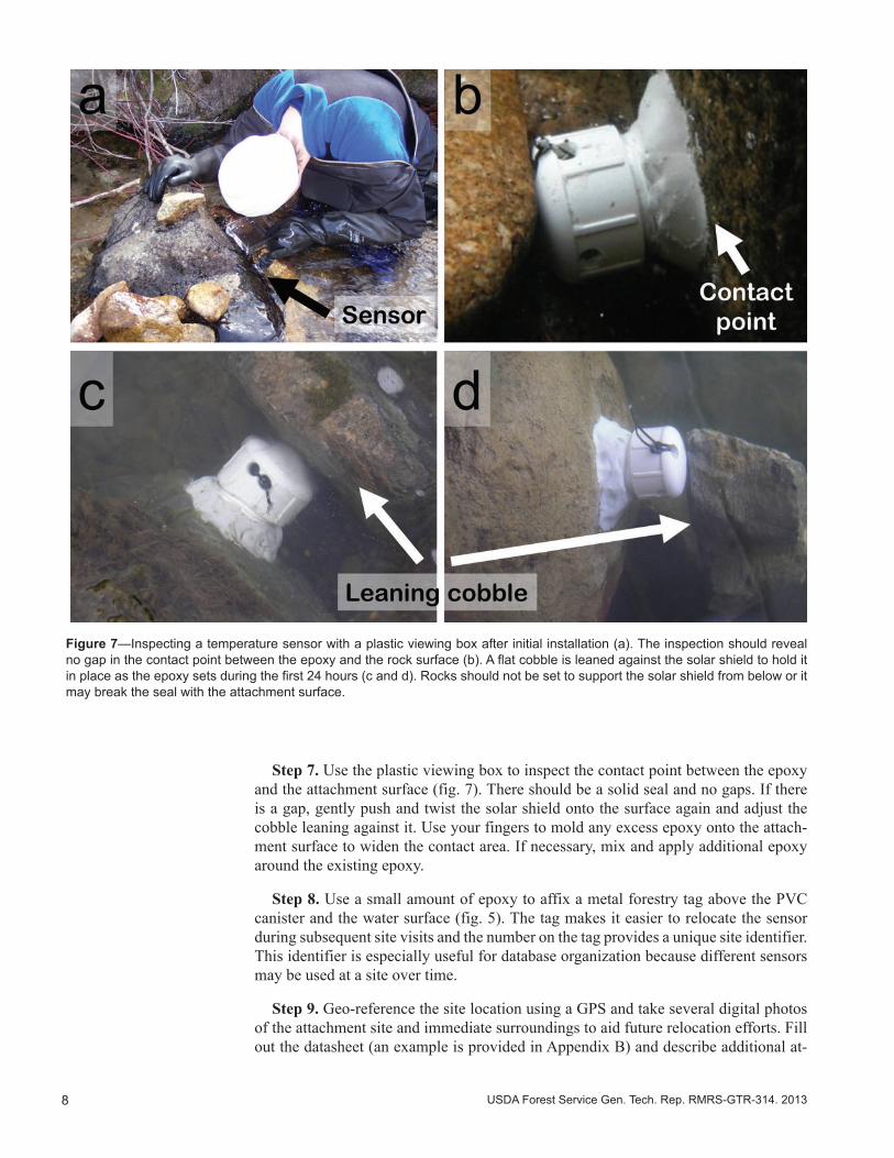
Step 6. Hold the PVC canister with epoxy under water so that air is forced out of the assembly. Study the cleaned attachment site to choose the best microsite, then push and slowly twist the assembly onto the attachment site. The assembly may (or may not) hold itself to the attachment surface at this point, so gently lean the cobble from Step 4 against the face of the solar shield to hold it in place as the epoxy sets during the first 24 hours (Figure 7). Important: lean cobble against assembly even if it initially holds itself or it may fall off before the epoxy sets. The cobble should lean directly into the PVC canister to provide a steady pressure that does not cause torque. Do not attempt to support the solar shield from below with cobbles or it may break the seal at the contact point between the epoxy and the attachment surface.

Figure 6—Preparing the Fox epoxy for use involves mixing equal amounts of the two components together for approxi-mately 1 minute until the color is uniform throughout. Fingers should be wetted before and during mixing to minimize epoxy sticking to gloves.


Step 7. Use the plastic viewing box to inspect the contact point between the epoxy and the attachment surface (fig. 7). There should be a solid seal and no gaps. If there is a gap, gently push and twist the solar shield onto the surface again and adjust the cobble leaning against it. Use your fingers to mold any excess epoxy onto the attach-ment surface to widen the contact area. If necessary, mix and apply additional epoxy around the existing epoxy.

Step 8. Use a small amount of epoxy to affix a metal forestry tag above the PVC canister and the water surface (fig. 5). The tag makes it easier to relocate the sensor during subsequent site visits and the number on the tag provides a unique site identifier. This identifier is especially useful for database organization because different sensors may be used at a site over time.

Step 9. Geo-reference the site location using a GPS and take several digital photos of the attachment site and immediate surroundings to aid future relocation efforts. Fill out the datasheet (an example is provided in Appendix B) and describe additional at-

Figure 7—Inspecting a temperature sensor with a plastic viewing box after initial installation (a). The inspection should reveal no gap in the contact point between the epoxy and the rock surface (b). A flat cobble is leaned against the solar shield to hold it in place as the epoxy sets during the first 24 hours (c and d). Rocks should not be set to support the solar shield from below or it may break the seal with the attachment surface.


tributes about the location (e.g., “sensor attached to rectangular rock 1m in diameter along left side of the channel”). Once back in the office, create and maintain a digital archive of the site photos.

If you are installing sensors with epoxy for the first time, consider doing several prac-tice installations under controlled conditions in the laboratory or office. It may also be useful to revisit the first few field installations soon after the initial installation (i.e., the next day or week) to gain confidence in the technique. The epoxy takes approximately 24 hours to set and a firm bond to the attachment surface should make it difficult to remove the PVC canister assembly at that time. If the assembly is not firmly attached or has fallen off the surface, simply recover the sensor and repeat steps 1 – 9 using a new PVC canister. Appendix C is a one-page summary of these nine steps and is useful as a field reference guide. To watch a training video of an epoxy sensor installation, see this YouTube video http://www.youtube.com/watch?v=vaYaycwfmXs&feature=youtu.be.

Data Retrieval and Site Maintenance

Monitoring sites should be visited periodically to maintain the sensor installation and retrieve temperature data. We attempt to revisit each site the year after establishment to confirm that the installation survived the annual flood and the sensor is functioning properly. Once a site is successfully established, future visits could occur annually or less frequently, depending on user preferences and the sensor’s deployment capacity (i.e., battery life and data storage). To retrieve data, simply remove the sensor from the PVC canister by unscrewing the cap, cut the cable tie holding the sensor in the cap, and transfer data to a data shuttle or field computer (Appendix D describes how to down-load a TidbiT v2 using a data shuttle). At this time, it is also useful to measure stream temperature with a NIST certified thermometer to serve as a calibration point to assess potential long-term drift in sensor measurements. To reinitiate data collection efforts, simply strap the sensor back into the cap of the PVC canister and screw it to the base. If the sensor is at the end of its service life, replace it with a new one in the same solar shield canister.

If the site was not established successfully and the sensor was lost, attempt to deter-mine the cause. Was the site vandalized, did a large flood significantly alter the channel bed, or did the sensor detach from the attachment surface due to a poor installation? Answers to those questions can inform how, or whether, another sensor installation is attempted at the site.

Results From Previous Sensor Installations

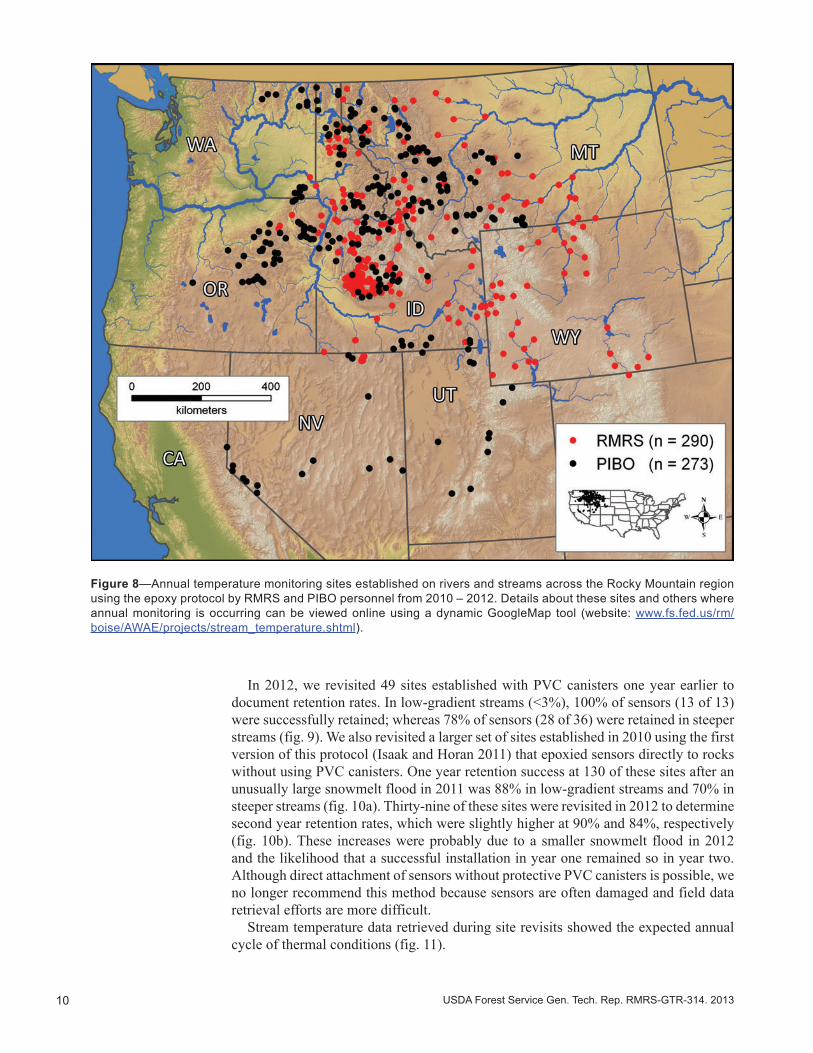
Working collaboratively with the U.S. Forest Service PIBO (PacFish/Infish Biological Opinion) stream monitoring program, we used the epoxy protocol to establish 563 annual temperature monitoring sites on rivers and streams across the Rocky Mountain region from 2010 – 2012 (fig. 8; Isaak 2012). Installations occurred in diverse environments that ranged from small, steep streams to larger systems like the Salmon, Snake, Green, and Yellowstone rivers. Sensors were installed successfully in a wide range of stream temperatures (2 – 20 °C), but the epoxy became noticeably less viscous and more fri-able toward the upper end of this temperature range. In especially warm streams, users should consider doing installations during cooler morning or evening hours to ensure the epoxy begins setting properly. Once experience was gained with the protocol, it required approximately 20 minutes to install a temperature sensor after locating a suit-able attachment site.


Figure 8—Annual temperature monitoring sites established on rivers and streams across the Rocky Mountain region using the epoxy protocol by RMRS and PIBO personnel from 2010 – 2012. Details about these sites and others where annual monitoring is occurring can be viewed online using a dynamic GoogleMap tool (website: www.fs.fed.us/rm/boise/AWAE/projects/stream_temperature.shtml).

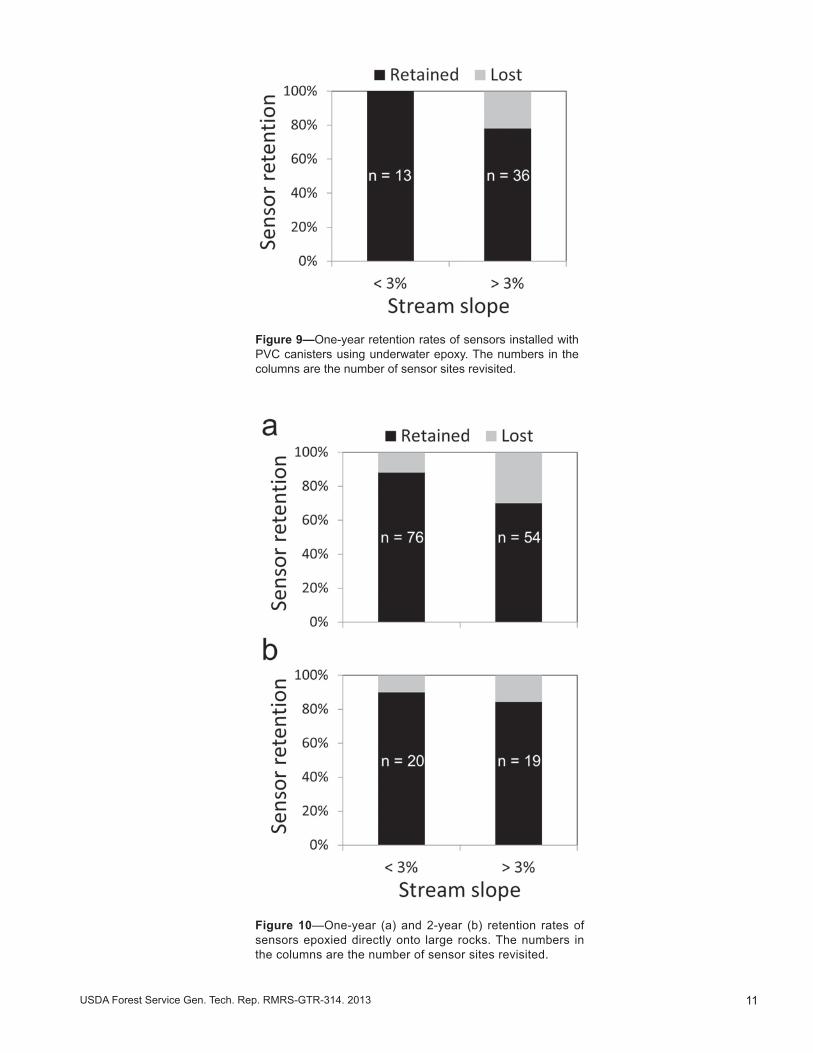
In 2012, we revisited 49 sites established with PVC canisters one year earlier to document retention rates. In low-gradient streams (<3%), 100% of sensors (13 of 13) were successfully retained; whereas 78% of sensors (28 of 36) were retained in steeper streams (fig. 9). We also revisited a larger set of sites established in 2010 using the first version of this protocol (Isaak and Horan 2011) that epoxied sensors directly to rocks without using PVC canisters. One year retention success at 130 of these sites after an unusually large snowmelt flood in 2011 was 88% in low-gradient streams and 70% in steeper streams (fig. 10a). Thirty-nine of these sites were revisited in 2012 to determine second year retention rates, which were slightly higher at 90% and 84%, respectively (fig. 10b). These increases were probably due to a smaller snowmelt flood in 2012 and the likelihood that a successful installation in year one remained so in year two. Although direct attachment of sensors without protective PVC canisters is possible, we no longer recommend this method because sensors are often damaged and field data retrieval efforts are more difficult.

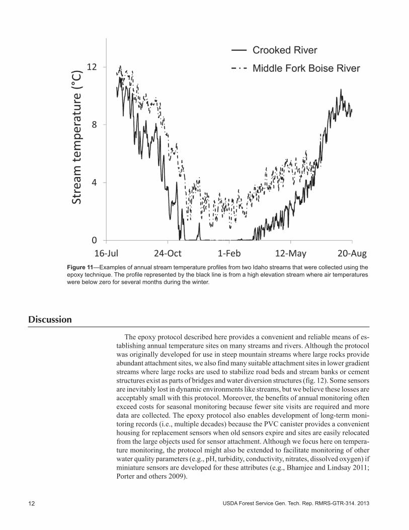
Stream temperature data retrieved during site revisits showed the expected annual cycle of thermal conditions (fig. 11).


Figure 9—One-year retention rates of sensors installed with PVC canisters using underwater epoxy. The numbers in the columns are the number of sensor sites revisited.

Figure 10—One-year (a) and 2-year (b) retention rates of sensors epoxied directly onto large rocks. The numbers in the columns are the number of sensor sites revisited.


Figure 11—Examples of annual stream temperature profiles from two Idaho streams that were collected using the epoxy technique. The profile represented by the black line is from a high elevation stream where air temperatures were below zero for several months during the winter.

Discussion

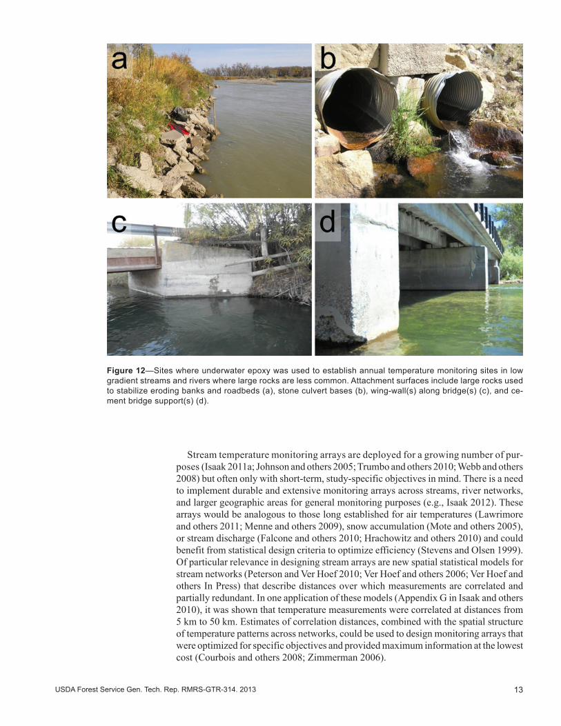
The epoxy protocol described here provides a convenient and reliable means of es-tablishing annual temperature sites on many streams and rivers. Although the protocol was originally developed for use in steep mountain streams where large rocks provide abundant attachment sites, we also find many suitable attachment sites in lower gradient streams where large rocks are used to stabilize road beds and stream banks or cement structures exist as parts of bridges and water diversion structures (fig. 12). Some sensors are inevitably lost in dynamic environments like streams, but we believe these losses are acceptably small with this protocol. Moreover, the benefits of annual monitoring often exceed costs for seasonal monitoring because fewer site visits are required and more data are collected. The epoxy protocol also enables development of long-term moni-toring records (i.e., multiple decades) because the PVC canister provides a convenient housing for replacement sensors when old sensors expire and sites are easily relocated from the large objects used for sensor attachment. Although we focus here on tempera-ture monitoring, the protocol might also be extended to facilitate monitoring of other water quality parameters (e.g., pH, turbidity, conductivity, nitrates, dissolved oxygen) if miniature sensors are developed for these attributes (e.g., Bhamjee and Lindsay 2011; Porter and others 2009).


Figure 12—Sites where underwater epoxy was used to establish annual temperature monitoring sites in low gradient streams and rivers where large rocks are less common. Attachment surfaces include large rocks used to stabilize eroding banks and roadbeds (a), stone culvert bases (b), wing-wall(s) along bridge(s) (c), and ce-ment bridge support(s) (d).

Stream temperature monitoring arrays are deployed for a growing number of pur-poses (Isaak 2011a; Johnson and others 2005; Trumbo and others 2010; Webb and others 2008) but often only with short-term, study-specific objectives in mind. There is a need to implement durable and extensive monitoring arrays across streams, river networks, and larger geographic areas for general monitoring purposes (e.g., Isaak 2012). These arrays would be analogous to those long established for air temperatures (Lawrimore and others 2011; Menne and others 2009), snow accumulation (Mote and others 2005), or stream discharge (Falcone and others 2010; Hrachowitz and others 2010) and could benefit from statistical design criteria to optimize efficiency (Stevens and Olsen 1999). Of particular relevance in designing stream arrays are new spatial statistical models for stream networks (Peterson and Ver Hoef 2010; Ver Hoef and others 2006; Ver Hoef and others In Press) that describe distances over which measurements are correlated and partially redundant. In one application of these models (Appendix G in Isaak and others 2010), it was shown that temperature measurements were correlated at distances from 5 km to 50 km. Estimates of correlation distances, combined with the spatial structure of temperature patterns across networks, could be used to design monitoring arrays that were optimized for specific objectives and provided maximum information at the lowest cost (Courbois and others 2008; Zimmerman 2006).


Another design consideration is the length of time that monitoring occurs at indi-vidual sites. Given the rarity of long-term temperature records for streams and rivers (Isaak and others 2012; Kaushal and others 2010), significant efforts need to be directed towards establishing and maintaining some sites more or less indefinitely. Where pro-tracted monitoring is not possible, however, other factors can inform decisions about the monitoring period. For example, in the absence of data, most information about a site’s thermal conditions will be obtained during the first year and patterns thereafter become increasingly redundant. A minimum monitoring period, therefore, might be 2 or 3 years, which ensures that a full seasonal cycle is recorded, as well as some of the inter-annual variation related to climatic variability driven by differences in air tem-peratures and stream discharge. Temperature records of this length facilitate short-term sensitivity analyses useful for understanding spatial variation in temperature changes and can serve as proxies for longer term trends associated with climate change (Kelleher and others 2012; Mohseni and others 1999; Trumbo and others 2010). These records also provide adequate calibration periods for models run at short time-steps (i.e., daily or weekly periods) that are useful for studies about fish growth, stream metabolism, or exceedance of water quality standards (Mohseni and others 1998; van Vliet and others 2011). Longer monitoring periods are required for studies designed to describe past or future temperature trends (Kaushal and others 2010; Webb and Nobilis 2007). In these studies, a significant portion of the inter-annual thermal variability at a site should be sampled to ensure that the effects of air temperature and discharge on stream temperatures are accurately estimated (e.g., Markovic and others 2013; Moatar and Gailhard 2006). Erickson and others (1999) estimated that 15 years of temperature monitoring were required in this situation, which Isaak and others (2012) also found to be a useful record length for accurate reconstructions of historical trends in the northwest United States.

Conclusion

It is a unique and exciting time for those interested in stream temperature monitoring and modeling. Climate change and other factors associated with human development and land management pose significant threats to the thermal integrity of many streams and rivers. Our ability to quantify those threats with accurate measurements of temperature dramatically increased in the early 1990s with the advent of inexpensive, miniature temperature sensors. The epoxy protocol described here facilitates expansion of moni-toring efforts to all seasons of the year so that annual monitoring and long-term records become common in streams. Those data will enable better environmental assessments, a richer understanding of thermal regimes akin to that for hydrologic regimes (Olden and Naiman 2010; Poff and others 1997; Poole and others 2004), and new scientific inquiries regarding the thermal ecology of aquatic species (McCullough and others 2009; Portner and Peck 2010).

For more information about stream temperature monitoring, modeling, or to access temperature databases, please visit the U.S. Forest Service stream temperature website (http://www.fs.fed.us/rm/boise/AWAE/projects/stream_temperature.shtml) or the Nor-WeST website (http://www.fs.fed.us/rm/boise/AWAE/projects/NorWeST.html).


References

Adams, M. 2013. Protocol for placement and retrieval of temperature data loggers in Idaho streams, ver-sion 2. Water Quality Monitoring Protocol—Report No. 10. Boise, ID: Idaho Department of Environ-mental Quality. 25 p.

Arrigoni, A. S.; Poole, G. C.; Mertes, L. A.; O’Daniel, S. J.; Woessner, W. W.; Thomas, S. A. 2008. Buff-ered, lagged, or cooled? Disentangling hyporheic influences on temperature cycles in stream channels. Water Resources Research. 44: W09418, doi:10.1029/2007WR006480.

Bhamjee R.; Lindsay, J. B. 2011. Ephemeral stream sensor design using state loggers. Hydrology and Earth System Sciences. 15:1009-1021.

Birkeland, S. 2001. EPA’s TMDL program. Ecology Law Quarterly. 28: 297-325.Courbois, J. Y.; Katz, S. L.; Isaak, D. J.; Steel, E. A.; Thurow, R. F.; Wargo Rub, A. M.; Jordan, C. E. 2008.

Evaluating probability sampling strategies for estimating redd counts: an example with Chinook salmon (Oncorhynchus tshawytscha). Canadian Journal of Fisheries and Aquatic Sciences. 65: 1814-1830.

Dunham, J. B.; Chandler, G.; Rieman, B. E.; Martin, D. 2005. Measuring stream temperature with digital dataloggers: a user’s guide. Gen. Tech. Rep. GTR-RMRS-150WWW. Fort Collins, CO: U.S. Department of Agriculture, Forest Service, Rocky Mountain Research Station.

Dunham, J. B.; Rosenberger, A. E.; Luce, C. H.; Rieman, B. E. 2007. Influences of wildfire and channel reorganization on spatial and temporal variation in stream temperature and the distribution of fish and amphibians. Ecosystems. 10: 335-346.

Erickson, T. R.; Mohseni, O.; Stefan, H. G. 1999. Required record length for a nonlinear weekly air-stream temperature regression model. Project Report Number 436. St. Anthony Falls: University of Minnesota, Engineering, Environmental and Geophysical Fluid Dynamics Laboratory..

Falcone, J. A.; Carlisle, D. M.; Wolock, D. M.; Meador, M. R. 2010. GAGES: a stream gage database for evaluating natural and altered flow conditions in the conterminous United States: Ecological Archives E091-045. Ecology. 91(2): 621.

Hrachowitz, M.; Soulsby, C.; Imholt, C.; Malcolm, I. A.; Tetzlaff, D. 2010. Thermal regimes in a large upland salmon river: a simple model to identify the influence of landscape controls and climate change on maximum temperatures. Hydrological Processes. 24: 3374-3391.

Isaak, D. J. 2011a. Stream temperature monitoring and modeling: Recent advances and new tools for managers., Fort Collins, CO: Rocky Mountain Research Station, Stream Systems Technology Center. Stream Notes: 1-7.

Isaak, D. J. 2011b. Thoughts on monitoring designs for temperature sensor networks across river and stream basins. Climate-Aquatics Blog #8 www.fs.fed.us/rm/boise/AWAE/projects/stream_temp/stream_ temperature_climate_aquatics_blog.html.

Isaak, D. J. 2012. NoRRTN (Northern Rockies River Temperature Network): an inexpensive regional river temperature monitoring network. Climate-Aquatics Blog #24 www.fs.fed.us/rm/boise/AWAE/projects/stream_temp/stream_temperature_climate_aquatics_blog.html.

Isaak, D. J.; Horan, D. L. 2011. An assessment of underwater epoxies for permanently installing temperature sensors in mountain streams. North American Journal of Fisheries Management. 31: 134-137.

Isaak, D. J.; Luce, C. H.; Rieman, B. E.; Nagel, D. E.; Peterson, E. E.; Horan, D. L.; Parkes S.; Chandler, G. L. 2010. Effects of climate change and recent wildfires on stream temperature and thermal habitat for two salmonids in a mountain river network. Ecological Applications. 20: 1350-1371.

Isaak, D. J.; Rieman, B. E. 2013. Stream isotherm shifts from climate change and implications for distribu-tions of ectothermic organisms. Global Change Biology. 19: 742-751.

Isaak, D. J.; Rieman, B. E.; Horan, D. 2009. A watershed-scale bull trout monitoring protocol. Gen. Tech. Rep. GTR-RMRS-224, Fort Collins, CO: U.S. Department of Agriculture, Forest Service, Rocky Moun-tain Research Station. 25 p.

Isaak, D. J.; Wenger, S. J.; Peterson, E. E.; Ver Hoef, J. M.; Hostetler, S.; Luce, C. H.; Dunham, J. B.; Kershner, J.; Roper, B. B.; Nagel, D.; Horan, D.; Chandler, G.; Parkes, S.; Wollrab, S. 2011. NorWeST: an interagency stream temperature database and model for the Northwest United States. U.S. Fish and Wildlife Service, Great Northern Landscape Conservation Cooperative Grant. Project website: www.fs.fed.us/rm/boise/AWAE/projects/NorWeST.html.

Isaak, D. J.; Wollrab, S.; Horan, D; Chandler, G. 2012. Climate change effects on stream and river tem-peratures across the Northwest U.S. from 1980 – 2009 and implications for salmonid fishes. Climatic Change. 113: 499-524.

Johnson, A. N.; Boer, B. R.; Woessner, W. W.; Stanford, J. A.; Poole, G. C.; Thomas, S. A.; O’Daniel, S. J. 2005. Evaluation of an inexpensive small diameter temperature logger for documenting ground water-river interactions. Ground Water Monitoring & Remediation. 25: 68-74.


Kaushal, S. S.; Likens, G. E.; Jaworski, N. A.; Pace, M. L.; Sides, A. M.; Seekell, D.; Belt, K. T.; Secor, D. H.; Wingate, R. L. 2010. Rising stream and river temperatures in the United States. Frontiers in Ecology and the Environment. doi:10.1890/090037.

Kelleher, C.; Wagener, T.; Gooseff, M.; McGlynn, B.; McGuire, K.; Marshall, L. 2012. Investigating controls on the thermal sensitivity of Pennsylvania streams. Hydrological Processes. 26:771-785.

Lawrimore, J. H.; Menne, M. J.; Gleason, B. E.; Williams, C. N.; Wuertz, D. B.; Vose, R. S.; Rennie, J. 2011. An overview of the global historical climatology network monthly mean temperature dataset, Version 3. Journal of Geophysical Research-Atmospheres. 116: D19121, doi:10.1029/2011JD016187.

Markovic, D.; Scharfenberger, U.; Schmutz, S.; Pletterbauer, F.; Wolter, C. 2013. Variability and altera-tions of water temperatures across the Elbe and Danube River Basins. Climatic Change. doi: 10.1007/s10584-013-0725-4.

Mauger, S. 2008. Water temperature data sensor protocol for Cook Inlet salmon streams. Cook Inletkeeper, Homer, Alaska. 10 p.

McCullough, D. A.; Bartholow, J. M.; Jager, H. I.; Beschta, R. L.; Cheslak, E. F.; Deas, M. L.; Ebersole, J. L.; Foott, J. S.; Johnson, S. L.; Marine, K. R.; Mesa, M. G.; Petersen, J. H.; Souchon, Y.; Tiffan, K. F.; Wurtsbaugh, W. A. 2009. Research in thermal biology: burning questions for coldwater stream fishes. Reviews in Fisheries Science. 17: 90-115.

Menne, M. J.; Williams, C. N.; Vose, R. S. 2009: The United States historical climatology network monthly temperature data - Version 2. Bulletin of the American Meteorological Society. 90: 993-1007.

Moatar, F.; Gailhard, J. 2006. Water temperature behaviour in the River Loire since 1976 and 1881. Comptes Rendus Geoscience. 338: 319-328.

Mohseni, O.; Erickson T. R.; Stefan, H. G. 1999. Sensitivity of stream temperatures in the United States to air temperatures projected under a global warming scenario. Water Resources Research. 35: 3723-3733.

Mohseni, O.; Stefan, H. G.; Erickson, T. R. 1998. A nonlinear regression model for weekly stream tem-peratures. Water Resources Research. 34: 2685-2692.

Moore, R. D.; Nelitz, M.; Parkinson, E. 2013. Empirical modelling of maximum weekly average stream temperature in British Columbia, Canada, to support assessment of fish habitat suitability. Canadian Water Resources Journal. doi:10.1080/07011784.2013.794992.

Moore, R. D. 2006. Stream temperature patterns in British Columbia, Canada, based on routine spot mea-surements. Canadian Water Resources Journal 31: 41–56.

Mote, P. W.; Hamlet, A. F.; Clark, M. P.; Lettenmaier, D. P. 2005. Declining mountain snowpack in western North America. Bulletin of the American Meteorological Society. 86: 39-49.

Neuheimer, A. B.; Taggart, C. T. 2007. The growing degree-day and fish size-at-age: the overlooked metric. Canadian Journal of Fisheries and Aquatic Sciences. 64: 375-385.

Olden, J. D.; Naiman, R. J. 2010. Incorporating thermal regimes into environmental flows assessments: modifying dam operations to restore freshwater ecosystem integrity. Freshwater Biology. 55: 86-107.

Peterson, E. E.; Ver Hoef, J. M. 2010. A mixed-model moving-average approach to geostatistical modeling in stream networks. Ecology. 91: 644-651.

Poff, N. L.; Allan, J. D.; Bain, M. B.; Karr, J. R.; Prestegaard, K. L.; Richter, B. D.; Sparks, R. E.; Strom-berg, J. C. 1997. The natural flow regime: a paradigm for river conservation and restoration. BioScience. 47: 769-784.

Poole, G. C.; Dunham, J. B.; Keenan, D. M.; Sauter, S. T.; McCullough, D. A.; Mebane, C.; Lockwood, J. C.; Essig, D. A.; Hicks, M. P.; Sturdevant, D. J.; Materna, E. J.; Spaulding, S. A.; Risley, J.; Deppman, M. 2004. The case for regime-based water quality standards. BioScience. 54: 155-161.

Porter, J. H.; Nagy, E.; Kratz, T. K.; Hanson, P.; Collins, S. L.; Arzberger, P. 2009. New eyes on the world: advanced sensors for ecology. Bioscience. 59: 385-397.

Portner, H. O.; Peck, M. A. 2010. Climate change effects on fishes and fisheries: towards a cause-and-effect understanding. Journal of Fish Biology. 77 :1745-1779.

Stevens, D. L.; Olsen, A. R. 1999. Spatially restricted surveys over time for aquatic resources. Journal of Agricultural Biological and Environmental Statistics. 4: 415-428.

Todd, A.S.; Coleman, M.A.; Konowal, A.M.; May, M.K.; Johnson, S.; Vieira, N.K.M.; Saunders, J.F. 2008. Development of new water temperature criteria to protect Colorado’s fisheries. Fisheries. 33:433-443.

Trumbo, B.; Hudy, M.; Smith, E. P.; Kim, D. Y.; Wiggins, B. A.; Nislow, K. H.; Dolloff, C. A. 2010. Sensitivity and vulnerability of brook trout populations to climate change. In: Wild Trout X: Conserving wild trout; Proceedings of the 10th annual wild trout symposium; Sept. 28-30, 2010; West Yellowstone, MT: 62-68.

U.S. Environmental Protection Agency (USEPA). In Press. Guidelines for continuous monitoring of temperature and flow in wadeable streams. EPA/6--/R-13/XXX. Washington, DC: National Center for Environmental Assessment, Air, Climate, and Energy Program.

van Vliet, M. T. H.; Ludwig, F.; Zwolsman, J. J. G.; Weedon, G. P.; Kabat, P. 2011. Global river tempera-tures and sensitivity to atmospheric warming and changes in river flow. Water Resources Research. 47: doi:10.1029/2010WR009198.


Ver Hoef, J. M.; Peterson, E. E.; Theobald. D. M. 2006. Spatial statistical models that use flow and stream distance. Environmental and Ecological Statistics. 13: 449-464.

Ver Hoef, J. M.; Peterson, E. E.; Clifford, D.; Shah, R. In Press. SSN: An R package for spatial statistical modeling on stream networks. Journal of Statistical Software.

Ward, W. 2011. Standard operating procedures for continuous temperature monitoring of fresh water rivers and streams, version 1. Washington State Department of Ecology Environmental Assessment Program.

Webb, B. W.; Hannah, D. M.; Moore, R. D.; Brown, L. E.; Nobilis, F. 2008. Recent advances in stream and river temperature research. Hydrological Processes. 22:902-918.

Webb, B. W.; Nobilis, F. 2007. Long-term changes in river temperature and the influence of climatic and hydrological factors. Hydrological Sciences. 52: 74-85.

Zimmerman, C.E.; Finn, J.E. 2012. A simple method for in situ monitoring of water temperature in substrates used by spawning salmonids. Journal of Fish and Wildlife Management. 3(2): 288-295.

Zimmerman, D. L. 2006. Optimal network design for spatial prediction, covariance parameter estimation, and empirical prediction. Environmentrics. 17: 635-652.


Appendix A. Materials Needed to Install an Annual Stream Temperature Monitoring Site Using Underwater Epoxy

Product Supplier Web Address Part number FOR INSTALLING SENSOR:Temperature sensor Onset Computer Corporation http://www.onsetcomp.com UTBI-001 TidbiT v2PVC solar shield canister, 1-1/2” Screw top and base

Spears http://www.spears.com/

Call Spears for a local distributor

1-1/2” PVC Schedule 40 Female Cap

1-1/2” x 3/4” PVC SCH 40 M x F Bushing

Underwater epoxy Fox Industries http://www.foxind.com

Call Fox to find a local distributor

FX-764 Splash Zone Epoxy

Jar: 60 ml (2 oz)Jar: 125 ml (4 oz)(optional, for epoxy)

Fisher Scientific Fisher ScientificOr use jars from the Dollar Store

02891B 02891C

Underwater viewing box Hoffman Manufacturing http://www.hoffmanmfg.com CONT79CMetal forestry tags(with numbers)

Forestry Suppliers http://www.forestry-suppliers.com 79142

Rubber glovesPlumber’s tapeWire brushCable ties, 4” FOR DOWNLOADING SENSOR IN THE FIELD:Underwater data shuttle Onset Computer Corporation http://www.onsetcomp.com U-DTW-1 Waterproof

Shuttle GENERAL FIELD EQUIPMENT:GPSCameraDatasheet


Appendix B. Sample Datasheet with Information to Record During Establishment of an Annual Temperature Monitoring Site


Appendix C. Field Reference Guide: 9 Steps for Installing a Temperature Sensor With Epoxy

1. Find a suitable attachment site that consists of either a large rock or cement bridge support. Suitable sites have flat downstream surfaces that are shielded during floods and have sufficient water depths to keep sensors submerged during low flows. Picking a good site is the most important part of a successful installation, so choose carefully! Do not move rocks into the stream to serve as attachment sites. If you are able to move a rock, it is too small!

2. Find a convenient working location near the attachment site and spread out the materi-als needed to perform the installation. Check sensor for blinking light to ensure that it is functioning. Record sensor serial number and metal forestry tag number on datasheet. Fasten the sensor into the cap of the solar shield canister and screw the cap onto the base.

3. Put on rubber gloves and use wire brush to clean the attachment site surface. Clean a large area to provide a variety of microsite choices when making the final installation. Clean an area that is below the low flow water surface, but several inches above the streambed to minimize the possibility that the sensor will be buried during subsequent floods.

4. Place a flat cobble within easy reach of the attachment site so that it can be leaned against the face of the PVC canister after installation.

5. Wet gloved fingers in the stream, scoop out equal amounts of white and black epoxy from each container (balls about the diameter of a quarter), then mix together until a uniform gray color is achieved (requires at least 1 minute). The final mass of epoxy should be about the size of a golf ball. Apply epoxy to the base of the PVC canister—molding it over the lip, but also leaving plenty of epoxy on the bottom for adhesion to the attachment surface.

6. Hold the PVC canister with attached epoxy under water so that air is forced out of the assembly. Study the cleaned attachment site to choose the best microsite, then push and slowly twist the assembly onto the attachment site. Gently lean the cobble from Step 4 against the face of the canister to hold it in place while the epoxy sets. Do this even if the PVC canister is initially holding itself or it may fall off!

7. Use the plastic viewing box to inspect the contact point between the epoxy and attach-ment surface. There should be a solid seal and no gaps. If there is a gap, gently push and twist the solar shield canister onto the surface again and adjust the cobble leaning against it. Use your fingers to mold any excess epoxy onto the attachment surface to widen the contact area. If necessary, mix and apply additional epoxy around the existing epoxy.

8. Attach forestry tag with a small amount of epoxy above the water surface on the downstream side of the attachment surface.

9. Record the site location on a GPS and record the coordinates on the data sheet. Take several photos of site and record any additional pertinent information on the datasheet.


Figure D1—An Onset data shuttle can be used with the TidbiT v2 to download temperature data from a sensor in the field. The data shuttle shows an amber light during data transfer (a), a green light after the download is completed successfully (b), and a red light if the data download fails (c). The data shuttle can store data from 63 TidbiT v2 sensors before the memory capacity is exceeded.

Appendix D. Downloading a TidbiT v2 Temperature Sensor Using a Data Shuttle

TidbiT v2s are easily downloaded in the field using a portable data shuttle that is also manufactured by Onset (Appendix A). The shuttle is waterproof, compact in size, and can store data from 63 TidbiT sensors before the memory capacity is exceeded. Important tip, do not change the data shuttle batteries in the field because this stops the shuttle’s internal clock and will prevent downloading of data. To download a sensor using the shuttle, follow these steps.

Step 1. Remove the TidbiT sensor from the PVC canister. Study the indicator light to ensure that it is blinking and the sensor has been functioning properly. Next, inspect the front to check that both LED bulbs are intact. TidbiTs with a broken LED bulb continue to function correctly and collect data, but the sensor cannot be downloaded in the field. Instead, the TidbiT must be returned to Onset for data retrieval, which costs ~$30 and requires destroying the sensor to extract the memory chip.

Step 2. If both LED bulbs are intact, press the TidbiT firmly into the adapter on the end of the data shuttle and squeeze the black lever to initiate the download (Figure D1). The amber light will begin blinking if the download is occurring properly (Figure D1a). If the download is not occurring, the red light will begin blinking (Figure D1c). Remove the shuttle, clean the surface of the TidbiT and check to ensure that debris did not interfere with shuttle engagement. Squeeze the lever to stop the blinking red light. Reinsert the TidBiT to the adapter on the data shuttle and reinitiate the download sequence again by squeezing the black lever.

Step 3. When a download completes successfully (~1 minute depending on the amount of data stored), the shuttle will re-launch the TidbiT with a blank memory and the green light will begin blinking (Figure D1b). Squeeze the black lever on the data shuttle to stop the green light from blinking and remove the TidbiT from the shuttle. Confirm that the indicator light on the front of the TidbiT is blinking and that the sensor is again collecting data. The sensor is now ready for redeployment.

Once all downloads to the shuttle are complete, it can be linked to a computer and data transferred using the Hoboware software available from Onset. For additional details, users should consult the manual that accompanies the data shuttle and practice using it with the TidbiT v2 in the office.

The Rocky Mountain Research Station develops scientific information and technology to improve management, protection, and use of the forests and rangelands. Research is designed to meet the needs of the National Forest managers, Federal and State agencies, public and private organizations, academic institutions, industry, and individuals. Studies accelerate solutions to problems involving ecosystems, range, forests, water, recreation, fire, resource inventory, land reclamation, community sustainability, forest engineering technology, multiple use economics, wildlife and fish habitat, and forest insects and diseases. Studies are conducted cooperatively, and applications may be found worldwide. For more information, please visit the RMRS web site at: www.fs.fed.us/rmrs.

Station Headquarters Rocky Mountain Research Station

240 W Prospect RoadFort Collins, CO 80526

(970) 498-1100

Research Locations

The U.S. Department of Agriculture (USDA) prohibits discrimination against its customers, employees, and applicants for employment on the bases of race, color, national origin, age, disability, sex, gender identity, religion, reprisal, and where applicable, political beliefs, marital status, familial or parental status, sexual orientation, or all or part of an individual’s income is derived from any public assistance program, or protected genetic information in employment or in any program or activity conducted or funded by the Department. (Not all prohibited bases will apply to all programs and/or employment activities.) For more information, please visit the USDA web site at: www.usda.gov and click on the Non-Discrimination Statement link at the bottom of that page.

Reno, NevadaAlbuquerque, New MexicoRapid City, South Dakota

Logan, UtahOgden, UtahProvo, Utah

Flagstaff, ArizonaFort Collins, Colorado

Boise, IdahoMoscow, Idaho

Bozeman, MontanaMissoula, Montana

To learn more about RMRS publications or search our online titles:

www.fs.fed.us/rm/publications

www.treesearch.fs.fed.us

Federal Recycling Program Printed on Recycled Paper

a simple protocol using underwater epoxy to install annual

Documents