A simple optical system for interpreting coherence

theory.

Damien P. Kelly1,2

1 Institut fur Mikro-und Nanotechnologien,

Macro-Nano,

Fachgebiet Optik Design,

Technische Universitat Ilmenau,

P.O. Box 10 05 65,

98684 Ilmenau,

Germany.

2 Oryx Optics Ltd,

19 The Elms,

Athlone,

Ireland.

damienpkelly@gmail.com

1

arX

iv:1

609.

0573

4v1

[ph

ysic

s.op

tics]

19

Sep

2016

A new theoretical technique for understanding, analyzing and developing

optical systems is presented. The approach is statistical in nature, where

information about an object under investigation is discovered, by examining

deviations from a known reference statistical distribution. A Fourier optics

framework and a scalar description of the propagation of monochromatic

light is initially assumed. An object (belonging to a known class of objects)

is illuminated with a speckle field and the intensity of the resulting scattered

optical field is detected at a series of spatial locations by point square law

detectors. A new speckle field is generated (with a new diffuser) and the

object is again illuminated and the intensities are again measured and noted.

By making a large number of these statistical measurements - an ensemble

averaging process (which in general can be a temporal or a spatial averaging

process) - it is possible to determine the statistical relationship between the

intensities detected in different locations with a known statistical certainty.

It is shown how this physical property of the optical system can be used

to identify different classes of objects (discrete objects or objects that vary

continuously as a function of several physical parameters) with a specific

statistical certainty. The derived statistical relationship is a fourth order

statistical process and is related to the mutual intensity of scattered light.

A connection between the integration time of the intensity detectors and

temporal coherence and hence temporal bandwidth of a quasi-monochromatic

light source is discussed. We extend these results to multiple wavelengths and

polarizations of light. We briefly discuss how the results may be extended to

non-paraxial optical systems.

c© 2016 Optical Society of America

2

1. Introduction

In this paper we develop a simple ‘thought-model’ to help us understand coherence theory

for scalar optical fields. This model will allow us to consider light with different coherence

and polarization states and which may contain many different contributing wavelengths.

We will examine how this light field interacts with some object and then how the resulting

scattered light is detected; specifically, we will examine point intensity detectors that

measure the intensity of the scattered light over a finite aquisition time. We will examine

this problem using a Fourier optics framework. A particular advantage of Fourier optics is

that the relative simplicity of the treatment allows one to develop intuitive models that

provide significant insight into the behaviour of optical systems [1–4].

Here, we assume that a scalar model of light propagation is valid; that there are no

current sources or charges in our medium; and hence that each vectorial component of

the electromagnetic field can be treated independently from the other components [1].

This implies that the different vectorial components do not interact with or ‘see’ each

other. Within the scalar description of light propagation, it is common to use diffraction

integrals to relate the complex scalar field in one plane, to the diffracted field, in an axially

displaced plane. Non-paraxial diffraction integrals such as the Rayleigh-Sommerfeld I and

II or the Kirchoff can be derived from the time-independent Helmholtz equation and

strictly speaking are correct only for propagation through a uniform medium with constant

refractive index. While these integrals are exact solutions for the scalar wave equation, the

analysis is easier still when the paraxial approximation is assumed. Now we can describe

light propagation using the Fresnel transform. A second and necessary part of our analysis

is to model the interaction of scalar field with some object. We imagine that if a field

is incident on the object, then the field ‘immediately after’ the object is calculated by

assuming the ‘Thin Element Approximation’ (TEA). The real physical dimensions of the

object are thus ignored, the object is imagined to be infinitely thin, and that the field

before and after the object are related to each other by multiplying the incident field with a

transmittance function. This type of approach is discussed at length by Goodman [1], and

will be adopted in the forthcoming analysis. These approximations are commonly used to an-

alyze speckle theory, aspects of coherence theory and statistical optics, see for example [5–8].

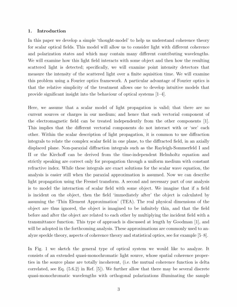
In Fig. 1 we sketch the general type of optical system we would like to analyze. It

consists of an extended quasi-monochromatic light source, whose spatial coherence proper-

ties in the source plane are totally incoherent, (i.e. the mutual coherence function is delta

correlated, see Eq. (5.6.2) in Ref. [5]). We further allow that there may be several discrete

quasi-monochromatic wavelengths with orthogonal polarizations illuminating the sample

3

LS plane

R X

object plane

extended LS [see (b)]

object

+D

-D -L

+L x 1 z 1 ( , )

x 2 z 2 ( , ) PID

x 3 z 3 ( , )

OSP Module: 1

OSP Module: 2

point detector array

(a)

spectrum of extended LS

U(R, λ)

λ

(b)

λ 3 λ 1 λ 2

Δλ

Δt

ATM

Fig. 1. (a) Schematic of the type of general optical system we are examin-

ing. The Light Source (LS) we are considering is a multi-wavelength extended

source, where the Amplitude Transmittance Mask (ATM) can be used to select

areas of light source that are used for the illumination of the sample. The light

from this source is modified by OSP Module 1 before it illuminates a sample

located in the object plane. The resulting scattered light is then collected by

OSP Module 2 before it is measured by an array of Point Intensity Detectors

(PID) that are both wavelength and polarization sensitive. The acquisition

time (integration time) of the detectors is ∆t. Inset (b) depicts the spectrum

of this extended LS.

4

simultaneously; we will use different transmittance masks to select specific parts of the

extended source to perform the illumination. The light emanating from this source is then

subject to a signal processing operation - by Optical Signal Processing (OSP) Module 1.

These OSP modules consist of combinations of lenses and sections of free space and can

be described using an LCT (see Section 1 of Ref. [9] or [10]). This light then illuminates

a sample that we are interested in examining that is situated in the object plane. The

interaction of the light and the sample is modelled using the TEA. Then the resulting

scattered light is once again subject to a signal processing operation - OSP Module 2 -

before its intensity is detected by an array intensity detectors. These intensity detectors

will, in general, be color and polarization selective so that multi-wavelength measurements

can be made simultaneously on different polarizations of the scattered and processed light.

We will be interested in relating the acquisition time of the intensity detectors, ∆t, to

coherence length of the individual discrete quasi-monochromatic illuminating light sources

and we note that the coherence length of the light is usually related to the inverse of its

spectral width and so to ∆λ in Inset (b) of Fig. 1, see for example Chap. 5 in Ref. [5].

In general this type of optical system is difficult to analyze due to all the different

aspects that need to be considered. Instead we propose to develop a simpler analytical

model or ‘Gedankenexperiment’ that may be used as a tool to understand how different

aspects of coherence theory, object detection, signal processing and electronic detection

interact with each other. An optical system that could fulfill this role is depicted in Fig.

2. There are several differences between this optical system and the more general one

depicted in Fig. 1. First this simpler system uses an optical Fourier transform to process

the illuminating light before it is incident on the object, and then a Fresnel transform is

used to model the propagation of the light after the object to the locations of the intensity

detector array. Secondly, we note that in this system the light we use is now considered to

be a perfectly mono-chromatic and spatially coherent plane wave which is incident on a

diffuser pair. This diffuser pair produces a Random Speckle Field (RSF) which serves as an

instance of the random interrogating signal or illumination field. The statistical properties

of such a field have been examined by many different authors [5, 7, 10–16]. A speckle field

follows well known statistical distributions for its intensity and phase distributions.

Suppose we move one of these diffusers, it is possible to generate a new and statisti-

cally independent field. While this second speckle field is completely different from the first

field it will have identical statistical properties. Other authors have examined the time

dependent statistical properties as these diffusers are moved relative to each other [17–21].

It is possible to determine a definite statistical relationship between the intensities at

5

different locations. Alternative methods for producing a similar effect to the diffuser pair

illumination are discussed here [22].

Having established these known statistical properties for a speckle field, we now con-

sider what happens to this known statistical distribution when an object (which we

think of as a symbol or message) is inserted into the optical path. It is expected that

the optical field interacts with the sample and modifies the statistical properties of the

scattered field [23, 24]. Hence by measuring changes in the resulting statistical distribution

we can identify the object under investigation. We can perform this measurement in

some cases using a single speckle field for illumination and by making a series of spatial

averages - spatial averaging. Alternatively we can illuminate the object with a sequence of

random speckle fields and perform a time averaging operation as is discussed here [17,18,25].

In the following section we derive a mathematical description of the optical system

in Fig. 2, deriving the relevant equations that follow from the assumptions we have just

outlined. In Section 3, we examine the characteristics of the resulting equations and derive

a correlation function - that is very similar to the mutual coherence function of discussed

by Goodman in Ref. [5]. Our correlation function however also depends on the nature of

the ATM in Fig. 2. Some specific calculated examples are presented for a range of different

objects. And we shall see that the analysis naturally extends to include partially coherent

effects, including the relationship between ∆t and ∆λ identified in Fig. 1. In Section 4, we

link the accuracy of our mathematical model to practical experimental measurements. In

Section 5, we discuss how these results can be extended and used to identify objects from

particular types of classes of objects. We discuss two forms of this problem: (i) Where the

objects come from a finite set of unique discrete objects; for example the set consisting of

either a lens or a grating, and (ii) Where the objects are described using a basis set and can

change continuously as a function of several physical parameters; this could be a lens with a

continually varying focal length. We find that a-priori information about the nature of the

object is essential so that different objects can be distinguished from each other. In Section

6, we discuss how the scalar analysis presented can be extended to include polarization

effects and different wavelengths of light. These results are exact within the assumptions we

have made and in the conclusion we briefly discuss how these could be extended to other

models of optical propagation and to models of the interaction of light and material.

2. The optical system

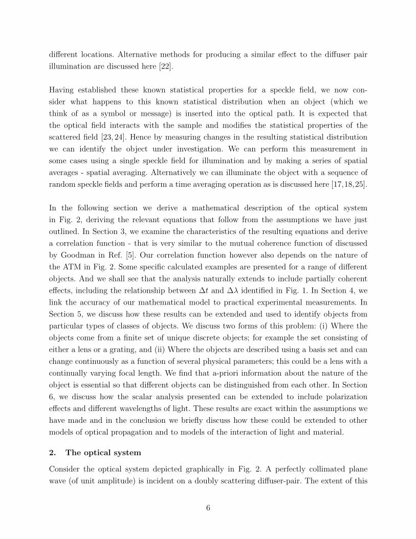
Consider the optical system depicted graphically in Fig. 2. A perfectly collimated plane

wave (of unit amplitude) is incident on a doubly scattering diffuser-pair. The extent of this

6

diffuser-pair is limited by a hard aperture with a width of 2D. Each diffuser is supposed to

be optically rough imparting phase changes that are uniformly distributed and greater than

2π. The surface profiles of the diffusers are modeled with two separate continuous functions.

Since these two surface profile functions describe two different diffusers it is reasonable to

assume that they are statistically independent; however they can still have identical statistical

properties and this is now assumed. For example the width of the auto-correlation of each

surface profile would be the same. We further assume that immediately after the diffuser-

pair, only the phase of the incident plane wave is modified while the amplitude remains

constant. We thus write an expression for the field ‘just after’ the diffuser-pair as

V (R) = exp [jΦn (R)] pD (R) , (1)

where Φn (R) is a random function which changes the phase of V (R) for each position of R.

We note that j =√−1, and that the aperture function is defined in the following manner

pD (R) =

1, when |R| < D

0, otherwise.(2)

In preparation for later discussion we briefly consider the characteristics of this diffuser-pair.

We note that if one diffuser is moved relative to the other even by a very small amount - on

the order of the auto-correlation width of the diffuser surface profile - it will generate a new

field V (R) that is statistically independent from the previous field, see [26,27], also Chapter

3 and 6 from Ref. [7], and [15, 20, 21, 28, 29]. A rough estimate for the amount of relative

translation between the two diffusers is about 10 µm [25]. Hence for two different relative

positions of the diffusers we get two different phase functions, Φ1 (R) and Φ2 (R) which have

identical statistical properties but are statistically independent of each other. In practice it

is possible to generate a very large number of these statistically independent phase functions

by moving the diffusers relative to each other and this fact is reflected in our notation where

the subscript ‘n’ in Φn (R) indicates a particular instance of a random phase function. We

now briefly consider the power of V (R), which can be calculated according to

PDP =∫ ∞−∞

V (R)V ∗(R)dR

= 2D. (3)

A spatial filtering operation is then implemented on on V (R) with a pinhole mask, see

Fig. 2, and hence only a portion of V (R) is allowed to propagate into the optical system.

Initially this pinhole mask will consist only of a single pinhole, however later in the text we

will generalize this expression by adding more pinholes to the mask and then extending the

analysis so that a continuum of point sources can be considered. Generally then we use an

7

diffuser plane

R X (OFT module)

x 1 z 1 ( , )

x 2 z 2 ( , ) PID

object plane

plane wave

diffuser pair

object

+D

-D -L

+L

(Fresnel transform)

ATM

Fig. 2. Optical setup for generating a speckle field. A plane wave is incident on

a diffuser and the phase of the field is randomized. The field behind the diffuser

is a Random Speckle Field (RSF). This field is Fourier transformed by a Kohler

lens and illuminates the target located in the X plane. The resulting scattered

intensity is measured at locations P1 and P2 by Point Intensity Detectors

(PID). Inset (i) depicts the zoomed in section A. To calculate the complex

amplitude at P3 one must consider the contribution at each point (several are

depicted) in the diffuser plane. Inset (ii) is the zoomed in section B. The diffuser

consists of two Rough Surfaces (RS). RS1 can rotate or translate relative to

RS2 to produce statistically independent speckle fields. Points P1 and P2 are

spatially located at (x1, z1) and (x2, z2) respectively.

8

Amplitude Transmittance Mask (ATM) to select appropriate areas of the source to illuminate

the object. This first part of the optical system, the illuminating optics, is modeled as an

ideal Fourier transforming system [1], where the lens is assumed to be both ‘thin’ and infinite

in extent [3,4,30]. For incoherent light sources this configuration is sometimes referred to as

Kohler illumination. We now write an expression for the resulting field that illuminates the

target situated in the object plane,

U (X) = Kf

∫ ∞−∞

V (R)δ (R−∆1) exp

(−j2πRX

λf

)dR

= Kf exp (jφ1) exp

(−j2π∆1X

λf

)(4)

where the constant Kf = 1/√jλf will be dropped for notational convenience from here on.

The pinhole in Fig. 2 is modeled as a Dirac delta point source located at R = ∆1 in the

diffuser plane. The wrapped phase value, φn1 = Φn(∆1), is a uniformly distributed random

variable lying between 0 and 2π. If we were to move the diffuser-pair relative to each other,

then a new value of φn1 would be generated, which would again be a uniformly distributed

random variable lying between 0 and 2π. Again for notational simplicity we will suppress

the ‘n’ superscript and refer simply to φ1.We recognize that Eq. (4) is a propagating plane

wave with a random phase, i. e.

U (X) = exp (jφ1) exp (−j2πfx1X) , (5)

with fx1 = ∆1/ (λf).

Let us describe the target in the object plane as O(X) such that

O (X) = O (X)U (X) . (6)

U(X) illuminates the object and the resulting scattered field propagates into the volume

behind the target plane where its intensity is recorded at two different locations by the

detectors, P1 and P2. These detectors record the intensity at a single point and hence we

ignore any spatial averaging effects caused by the finite size of the detector area [19,31]. Let

us first consider how to use the Fresnel transform to calculate the diffracted object field,

uz(x), under normal illumination

uz(x) = FSTz O(X) (x)

uz(x) = Kz

∫ ∞−∞

O(X) exp[jπ

λz(x−X)2

]dX, (7)

where Kz = (1/√jλz), λ the wavelength of the light, z is the propagation distance. In

practice we expect that O(X) will have a finite extent. We can write this explicitly then in

9

the following form O(X) = T (X)pL(X) and where pL(X) is an aperture function [defined

in the same manner as Eq. (2)] that defines the extent of the target in the object plane

and where T (X) describes the mathematical form of the target under examination. We now

make use of the ‘modulation’ property of the Fresnel transform. Given that

fz(x) = FSTz F (X) (x),

then the following relationship holds

FSTz F (X) exp (j2πρX) (x) = fz(x− λzρ) exp (j2πρx) exp (jφzc) ,

(8)

where φzc = −jπρ2λz, [32–34]. With this result we can thus find a general expression for

FSTzO(X)

(x),

uz(x,∆1) = exp (jφ1)uz(x− λzfx1) exp (j2πfx1x) exp (jφzc)

= exp (jφ1)uz

(x− z

f∆1

)exp (j2πfx1x) exp (jφzc) (9)

We now rewrite Eq. (9) in the following manner

uz(x,∆1) = exp (jφ1) a

(x− z

f∆1

)exp

[jΘ

(x− z

f∆1

)], (10)

where a(x) = |uz(x)| and where Θ(x) = arg uz(x) exp (j2πfx1x) exp (jφzc).

If we have an intensity detector situated at x = x1, z = z1, then as we physically

shift our pinhole over the range −D ≤ ∆1 ≤ D, we will measure intensity values of a2(x)

over the spatial range (x1 − zfD) ≤ x ≤ (x1 + z

fD). Hence we can scan the intensity of the

diffracted field over the detector by varying the location of the pinhole in the diffuser-pair

plane. Alternatively, we could move the detector position. We note that we would be unable

to determine from intensity measurements alone whether the pinhole was being scanned

over the diffuser-pair or whether the pinhole was stationary and the detector was moved.

This is not true of the complex amplitude due to the various factors in Eq. (9). We shall

return to this discussion in Section 3 and consider some implications for measuring the

power of the object field.

2.A. Addition of a second pinhole

We are now going to increase the complexity of the problem slightly by adding a second

pinhole, situated at R = ∆2, to the pinhole mask. Since we are dealing with a linear system

this means we can simple add the contribution from this second point source to the equations

10

we have derived above. Let us refer to the complex amplitude at the location P1 = (x1, z1)

as

u(P1) = uz=z1(x1,∆1) + uz=z1(x1,∆2)

= exp (jφ1) a

(x1 −

z1

f∆1

)exp

[jΘ

(x1 −

z1

f∆1

)]

+ exp (jφ2) a

(x1 −

z1

f∆2

)exp

[jΘ

(x1 −

z1

f∆2

)], (11)

which we rewrite again for simplicity as

u(P1) = exp (jφ1) a1 exp(jα1) + exp (jφ2) a2 exp(jα2). (12)

In a similar manner we can write that

u(P2) = exp (jφ1) b1 exp(jβ1) + exp (jφ2) b2 exp(jβ2). (13)

We are now in a position to examine in more detail the question of the intensities, I(P1) and

I(P2), recorded by the detectors. We begin by noting the following cumbersome relationship

I(P1)I(P2) = u(P1)u∗(P1)u(P2)u∗(P2)

= a21b

21 + a2

2b21 + a2

1b22 + a2

2b22

+2a1a2b21 cos (α1 − α2 + φ1 − φ2) + 2a1a2b

22 cos (α1 − α2 + φ1 − φ2)

+2a21b1b2 cos (β1 − β2 + φ1 − φ2) + 2a2

2b1b2 cos (β1 − β2 + φ1 − φ2)

+4a1a2b1b2 cos (α1 − α2 + φ1 − φ2) cos (β1 − β2 + φ1 − φ2) . (14)

2.B. Ensemble averaging

Eq. (14) describes the product of the intensities located at P1 and P2 for a given position

of the diffuser-pair. If the diffuser-pair were displaced relative to each other by a significant

amount (greater than the auto-correlation width of the surface function of the diffusers)

we should expect the intensity values I(P1), I(P2) and their product I(P1)I(P2) to change,

due to the fact that φn1 and φn2 are dependent on the relative diffuser-pair position. And

each time one of the diffusers in the diffuser-pair is moved relative to the other, then φn1and φn2 take on new and statistically independent values. Using angled brackets to denote an

ensemble average over a very large (strictly speaking an infinite) number relative diffuser-pair

positions, it can be shown that

〈I(P1)I(P2)〉 = a21b

21 + a2

2b21 + a2

1b22 + a2

2b22

+2a1a2b1b2 cos (α1 − α2 − β1 + β2) (15)

11

We now wish to extend the result in Eq. (15) so that N point sources in the diffuser-pair

plane can be considered together. It can be shown that the general form for this relationship

is given by

〈I(P1)I(P2)〉 = DC + CT, (16)

where

DC =

(N∑n=1

a2n

)(N∑n=1

b2n

), (17)

and

CT =N∑m=1

N∑n=m+1

amanbmbn cos (αm − αn − βm + βn)

. (18)

We would now like to extend the discrete analysis of N contributing point sources so that a

continuum of contributing point sources can be considered. Hence we shall rewrite Eq. (17)

and Eq. (18) in integral form where we shall integrate over that area of the source plane

that is allowed to contribute to the illumination of the object, i.e. we shall integrate over the

ATM,

DC =

[∫ATM

a2

(x1 −

z1

fR1

)dR1

] [∫ATM

b2

(x2 −

z2

fR2

)dR2

](19)

and

CT =∫ATM

∫ ATM

R1

a

(x1 −

z1

fR1

)b

(x2 −

z2

fR1

)a

(x1 −

z1

fR2

)

× b

(x2 −

z2

fR2

)cos [α(R1)− α(R2)− β(R2) + β(R1)] dR2dR1 (20)

This concludes our initial analysis of the experimental system depicted in Fig. 2.

3. The correlation function

We have just examined the intensity the detectors at P1 and P2 would measure. We would

now like to consider some aspects of the power of the detected field and then to examine the

definition of a correlation function that we will later use to identify specific objects.

3.A. Power illuminating the object

We saw from Eq. (3) that the total maximum power allowed into the optical system by

the source is given by 2D. This power will of course be reduced if source plane is stopped

12

down with the ATM. Often when analyzing speckle systems the diffuser surface is assumed

to be delta correlated, i.e. the auto-correlation of V (R) is a Dirac delta function. This

assumption greatly simplifies both speckle analysis and coherence theory, however it can

lead to an unphysical result, see the discussion in Section 2 of Ref. [21]. For example if the

diffuser were in fact delta correlated, then the power of the source would be diffracted over

an infinite extent in the illumination plane. This would imply that the maximum power

2D would be spread over an infinite extent with the result that very little power would in

fact pass through the object plane with its finite extent of 2L. And hence very little power

would be measured at the detector locations, P1 and P2.

However, in practice diffusers do not have a surface roughness function whose auto-

correlation is delta correlated. Hence the light scattered by the diffuser only extends over a

finite region in the object plane. There is a discrepancy between the theoretical model and

the experimental situation. It has the following manageable implications. In the previous

section we noted that each contributing point source had a unique and random phase value

φ(R) associated with it. If the auto-correlation of V (R) is not delta correlated then the same

random phase value will make several weighted contributions to the ensemble averaging

process. A good balance between the important simplifying theoretical assumption [that

the source plane (diffuser) has a surface roughness function that is delta correlated or the

extended light source has a delta correlated mutual coherence function] and ensuring that

the actual physical experiment is correctly modelled would be to ensure that the average

intensity at the object edges is approximately the same as the average intensity illuminating

the center of the object, i.e. the delta correlated assumption should be accurate provided

that:

〈U(0)U∗(0)〉 = 〈U(L)U∗(L)〉 = 〈U(−L)U∗(−L)〉 . (21)

This will also ensure that a sufficient amount of power passes through the object plane and

can be detected. Thus the power that then passes through the object plane is given by the

following expression:

Ptot =∫ L

−LO(X)O∗(X)dX, (22)

while the power of the field after the object when it is illuminated with only a single con-

tributing point source and hence a single plane wave is given by

Pobj =∫ L

−LO(X)O∗(X)dX. (23)

We will shortly use this power value, Pobj, to identify two different types of illumination

conditions. First however we shall consider the extent of uz(x) in the measurement plane

using power considerations.

13

3.B. Space-bandwith product of the object

We begin by making a general observation about uz(x) that is related to the spatial frequency

content and spatial extent of the target, O(X). We first note that Eq. (8) is a standard Fresnel

diffraction problem that has been analyzed by many authors [?,34,35], however it is difficult

to make any comments about the form of uz(x) without first making some assumptions about

O(X). We can say that O(X) is limited in spatial extent by the aperture function pL(X).

It then automatically follows that the spatial extent of uz(x) is in a strict mathematical

sense infinite [32]. It also follows that the spatial frequency extent O(X), as given by its

Fourier transform, is infinite [32]. At this point it is useful to consider the Space-Bandwidth

Product (SBP) of the signal O(X) which can be used to define a region in phase space where

a significant percentage of the signal’s power resides [?, 2, 34, 36–39]. Defining the Fourier

transform as

f(v) = FT f(X)f(v) =

∫ ∞−∞

f(X) exp (−j2πvX) dX, (24)

and the inverse transform as

f(X) = IFTf(X)

f(X) =

∫ ∞−∞

f(v) exp (+j2πvX) dv, (25)

it is possible to determine O(v) the Fourier transform of O(X). We expect from Parseval’s

theorem [40] that the power in the spatial and Fourier domains to be conserved so that

Pobj =∫ ∞−∞|O(v)|2dv. (26)

In practical cases however we are able to limit the extent of integration in the Fourier domain

to a finite region, −Γ ≤ v ≤ Γ such that

PR× Pobj =∫ Γ

−Γ|O(v)|2dv. (27)

PR has a value close to arbitrarily close to unity. The product of 2L times the spatial

frequency extent, 2Γ, is used to define the SBP of O(X). Once this has been established we

can also determine the effective Spatial Extent (SEz) of uz and we now refer the reader to

the following papers for more detail, [2, 34,36–39].

3.C. Power in the sequentially illuminated target

In Section 2, we observed that for a given position P1, it is possible to detect a2(x) over

the spatial range (x1 − z1fD) ≤ x ≤ (x1 + z1

fD) by moving the location of the pinhole ∆1,

14

see Fig. 2. Now we observe that if SEz lies within the range (x1 − z1fD) ≤ x ≤ (x1 + z1

fD)

then we can directly measure the total power of uz(x) by sequentially illuminating the target

and summing the resulting detected intensities. This must give a total power of Pobj which

is calculated from Eq. (23). If we again simplify our notation and emphasize the sequential

nature of this measurement, we would first detect the following intensity for one contributing

diffuser-pair point source

uz(x,∆1) = exp (jφ1) a1 exp(α1),

(28)

and

uz(x,∆2) = exp (jφ2) a2 exp(α2),

(29)

and so on. Summing all of these together we get,

Pobj = a21 + a2

2 + a23 + ... (30)

These observations also provide some insight into the interaction of speckle size and the

target under illumination. If in fact, SEz > 2Dz/f , then the power measurement we just

described will result in a lower estimate for Pobj. For the measurement to be follow Eq. (30)

the Kohler diameter must be sufficiently wide. We finally observe that if the pinhole mask

were removed from the optical system, see Fig. 2, then our target would be illuminated with

a speckle field, where the characteristic speckle size is given by λf/(2D), [5, 19].

3.C.1. Illumination conditions: CPDR

We can use the sequential illumination experiment just described to distinguish between two

types of detection schemes. If a detector measures a power given by Pobj then it is said to be

located in a Complete Power Detection Region (CPDR). Within this scheme a correlation

function that we shall define shortly, will always have a maximum value of unity when P1

and P2 are placed in the same location.

3.C.2. Illumination conditions: FPDR

It is not always necessarily desirable to have this property in the detection scheme. Sometimes

we can find out more information about a particular object or class of objects when they are

illuminated with different ATM’s as in Fig. 1 and Fig. 2. In this instance the detectors are

placed in a Fractional Power Detection Region (FPDR) and hence SEz does not lie within

the range (x1 − z1fATM) ≤ x ≤ (x1 + z1

fATM). The correlation function may sometimes

obtain values greater than unity, an effect that is seen in some doubly scattering speckle

phenomenon, [7, 21, 28].

15

3.D. Defining the correlation function

We begin by rewriting Eq. (18) in a slightly different form:

CT =N−1∑m=1

[N−m∑n=1

anan+mbnbm+n cos (αn − αn+m − βn + βm+n)

]. (31)

This form again involves a double summation, and we initially are going to concentrate on

the summation that is in square brackets above. As m increases the number of contributing

elements in the second summation decreases. We remember that the subscript on each of

the elements of the summation refers to the location of the contributing point source in

the diffuser-pair plane. When m = 1 we can see that each of the contributing elements are

neighboring points in the diffuser plane, and there are N − 1 terms. When m = 2 however

the first point source is linked with the third point source, the second with the fourth and

so on, such that there are N − 2 terms. It perhaps easier to see this effect in the following

illustrative table for five point sources, where the cos(·) variable serves as a place-holder for

the cosine terms from Eq. (31).

m n=1 n=2 n=3 n = 4 n = 5

1 a1a2b1b2 cos(·) a2a3b2b3 cos(·) a3a4b3b4 cos(·) a4a5b4b5 cos(·) a5a6b5b6 cos(·)2 0 a1a3b1b3 cos(·) a2a4b2b4 cos(·) a3a5b3b5 cos(·) a4a6b4b6 cos(·)3 0 0 a1a4b1b4 cos(·) a2a5b2b5 cos(·) a3a6b3b6 cos(·)4 0 0 0 a1a5b1b5 cos(·) a2a6b2b6 cos(·)5 0 0 0 0 a1a6b1b6 cos(·)

For a given value of N contributing point sources it is possible to estimate the num-

ber of CT terms with the following formula: (N − 1)N + N/2. The number of terms from

the DC contribution in this case is N2. Hence the ratio of DC terms to CT terms is given by

1− (2N)−1. In the limit as N →∞ then this ratio reduces to 1, indicating that 50% of the

total number of terms contribute to the DC component alone. The total number of terms is

given by 2N2 − N/2. The other terms then contribute to the CT in the following manner,

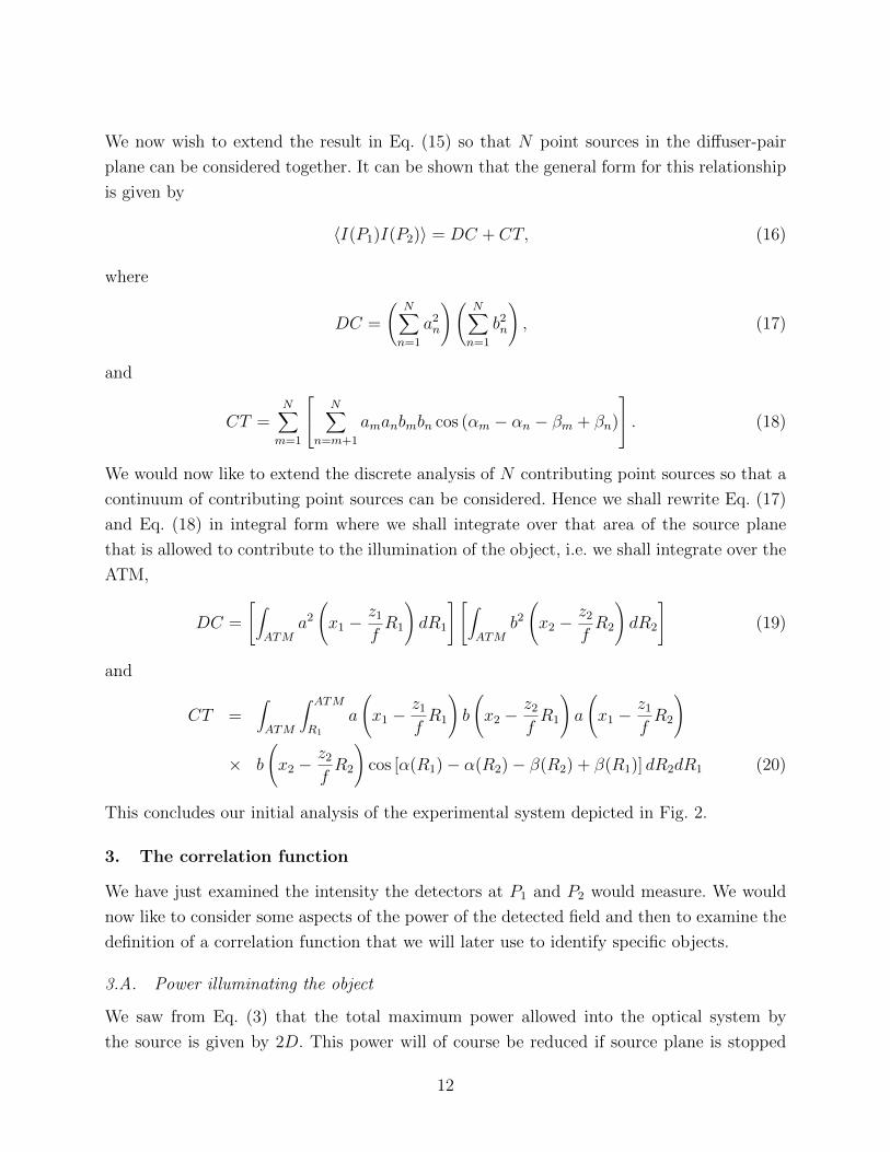
see Fig. 3. We now choose an CPDR for the location P1 using the experiment described in

Section 2.A and examine Eq. (31) when P1 and P2 are actually located in the same place.

When this happens the an and bn terms are the same with the effect of canceling the cosine

part of the cross-terms and Eq. (31) reduces to the following expression

N−1∑m=1

[N−m∑n=1

a2na

2n+m

], (32)

16

0.2 0.4 0.6 0.8 1.0Δ(n) (n+m)

2D

-0.4-0.2

0.20.40.60.81.0 CT terms

-4 -2 2 4 »x1-x2» HmmL0.2

0.4

0.6

0.8

1.0mHP1,P2L

(a) (b)

Fig. 3. (a) The number of terms that contribute to CT are distributed in the

following manner. There are more contributions from points that are located

near to each other spatially. (b) Decorrelation of the coherence field as P2 is

moved away from P1.

which if plotted as a function of spacing between contributing pinholes, exhibits the same

type of linear decay as the figure plotted in Fig. 2. If P1 and P2 are not in the same location

then an 6= bn and the cosine term: cos (αn − αn+m − βn + βm+n) comes back into play. We

thus choose the Normalization Factor (NF) to be

NF =√〈I(P1)I(P1)〉 〈I(P2)I(P2)〉, (33)

and now turn our attention to examining how CT terms behave as P2 is moved away from

P1 for an illustrative example. In this simulation we assume the following parameters, for the

optical system depicted in Fig. 2. We set λ = 500 nm, D = 1.25 mm, f = 20 cm, z1 = z2 = 20

cm, and the target under illumination in the object plane is a simple rectangular aperture,

pL(X), where L = 2.5 mm and N = 600. We define a correlation coefficient in the following

manner:

µ (P1, P2) =〈I(P1)I(P2)〉

NF, (34)

and plot the results in Fig. 3 (b). It is clear that as |x1 − x2| increases, the decorrelation

also increases. In Fig. 3(b), we also examine the decorrelation for two spatial locations,

|x1 − x2| = 1.125 µm and |x1 − x2| = 3 µm, and specifically plot the variation of

the corresponding CT terms in Fig. 3(a) which are the black and orange curves re-

spectively. As the P2 and P1 are separated spatially from each other, the cosine term:

cos (αn − αn+m − βn + βm+n) starts to add more and more ‘out of phase’ with each other

with the effect that area under the black and the orange CT curves is lower than the

maximum area that lies under the blue CT curve, i.e. when P1 = P2. Hence we understand

17

(b)

(c) (d)

(a)

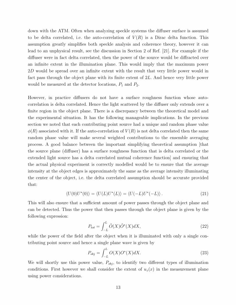
Fig. 4. Decorrelation of the coherence field as P2 is moved away from P1, see

text for details.

18

that the expected amount of decorrelation is directly related to the ratio of the area under

these two curves with a DC offset of 0.5.

In order to better appreciate some of the properties of the coherence function, µ(P1, P2),

we examine the 3-D distribution in Fig. 4 for a range of different detection locations. We

choose P1 and P2 such that we operate in a CPDR mode. Again the optical system has the

same parameters as those used to produce the plots in Fig. 3(b), however we now examine

µ(P1, P2) for several different objects defined in the following manner:

O(X) = pL(X) [exp (j2πfx1X) + g exp (j2πfx2X)] (35)

where g = 0 or 1 and fx1 and fx2 are the spatial frequencies associated with the linear

phase terms in Eq. (35). In Fig. 4(a) and (b), fx1 = 1200 lines/m and P1 is located on axis

with x1 = 0 and g = 0. In Fig. 4 (a) we see that µ(0, 0) has a value of unity. In Fig. 4(b)

we present a contour plot version of the same data, and it can be seen that µ(x1, x2) is

not symmetrical about the optical axis, and decreases as one moves to the bottom right of

the plot. This is due to the spatial frequency component fx1. In Fig. 4(c) we present the

same experiment however now the location of P1 has been changed and is now situated at

x1 = 120 µm. These properties can be used for alignment purposes. Finally in Fig. 4(d), we

set fx2 = fx1/2, and leaving x1 = 120 µm we can see ‘interference effects’ of the overlapping

spatial frequency components.

Thus we conclude that if the target under investigation is known, then it is possible

to calculate and predict the form of the correlation coefficient for any two detector pair

positions, P1 and P2. It is also possible to modify the form of the correlation coefficient by

changing the illumination of the source, for example by only illuminating with a specific

ATM or by sequentially illuminating with different ATM’s. If the illumination region is

‘stopped down’ then the detector signal, µ(P1, P2), can operate in a FPDR. As we shall see

this effect can be used as another means of finding out more information about the object

under investigation.

3.E. Partial coherence, acquisition time and spectral width of source

In the previous section we defined a correlation function µ(P1, P2). To measure this cor-

relation function in an experiment we need to measure the following ensemble average:

〈I(P1)I(P2)〉. This requires the following steps:

1. The intensity at P1 and P2 is recorded,

2. One of the diffusers in Fig. 2 is moved relative to the other diffuser and a new statis-

tically independent illumination field is generated,

19

3. Again the intensity values at P1 and P2 are recorded,

4. Steps 1-3 above are then repeated for a very large (strictly speaking infinite) number

of measurements. As we shall see in the following section only making a finite number

of measurements results in an expected and quantifiable error.

Since the diffusers are not moved during the detection of the light intensity, we define these

experimental steps as being a ‘coherent’ measurement.

We now consider however what would happen if the diffusers were moved rapidly

relative to each other and during the acquisition time (sometimes known as the integration

time) ∆t, of the intensity detector. If there were a very large number of statistically inde-

pendent realizations of the illuminating field within the integration time of the electronic

detector then the detected intensity at P1 would converge to the average intensity value, i.e.

〈I(P1)〉, and hence the correlation function, i.e. Eq. (34), would reduce to the following

µ (P1, P2) =〈I(P1)〉 〈I(P2)〉

NF. (36)

Thus the averaging operation, indicated with the angled brackets, operates not on the prod-

uct of the individual instances of intensity I(P1)I(P2), but rather on the averaged intensities

at the specific point detector locations. Since each detector would now only measure the

average intensity value, this is the opposite extreme of the ‘coherent’ measurement process

and hence we define this situation to be an ‘incoherent’ measurement.

Now we observe that if there are several statistically independent illuminations of

the object within the aquisition time of the detector that this is a partially coherent

measurement. Hence this concept of coherence depends on the number of statistically

independent measurements that are made within the aquisition time of the detector.

We would now like to extend our analysis so that a light source with a finite spec-

trum of wavelengths can also be considered. So we now examine what would happen

if we replaced the diffuser plane pair and the monochromatic light source that serve

to illuminate the sample in Fig. 2, and replaced them with an extended light source

instead. This light source will have a particular bandwidth ∆λ that is related to a partic-

ular temporal spectral width ∆ω by the following relationship for light in free space that

c = λω, where c is the speed of light in a vacuum and ω is the temporal frequency of the light.

Here we make a direct connection between a particular instance of our diffuser pair,

which produces a random phase distribution V (R) over the source plane and the instan-

taneous random (we also assume constant amplitude and random phase) distribution of

20

the extended source. How rapidly will the instantaneous random phase distribution of the

extended source change within the integration time of the detectors? We now make use of

some of the results outlined by Goodman, see Chap. 5 of Ref. [5] and also [6], and can define

a ‘coherence time’ τc for the light source. This ‘coherence time’ is related to the form of the

spectral profile, see for example Eq. (5.1-29) in Ref. [5].

In order for us to make a ‘coherent’ measurement, we require the speed of the opti-

cal detectors to be faster than τc in order to make a ‘coherent’ measurement as defined

above. Hence we have related the measurement technique in our simple optical system to

a light source that is no longer mono-chromatic. Other techniques for analyzing and using

partial coherence effects are discussed here [41–43].

4. Tchebycheff’s inequality, repeated trials and convergence.

The equations that we have been examining, particularly Eq. (14) to Eq. (31), are valid for

an ensemble averaging over a very large number of diffuser-pair positions. We remember that

we can generate a new and statistically independent realization of a speckle for illumination,

U(X), by moving the diffusers relative to each other by a small amount (order of the auto-

correlation of the surface profile), see Fig. 2. We now turn our attention to the convergence

properties of this averaging process and ask: With what accuracy can we estimate the actual

value of µ(P1, P2) when only a finite number, M , ‘realizations’ are used in the averaging

process? To address this question we turn to statistical methods to identify a ‘confidence

interval’, i.e. a percentage certainty that the estimated value lies within a specified narrow

range of the actual value. We follow the analysis given in Section 8.2, Chapter 8 of Ref. [44]

and adopt the notation-style given there for random variables; where y is a random variable

and yi is a specific instance of this random variable. We now model the detection of µ(P1, P2)

as a random process whereby we get the correct estimate plus a random error according to

y = µ(P1, P2) + e, (37)

where y is a random variable with an unknown probability distribution. For a given measure-

ment, yi, it represents our estimate of the actual value, µ(P1, P2) plus a random error, e,

which is related to the variance, σ, of µ(P1, P2) for different diffuser-pair realizations. We

calculate our best estimate, µE(P1, P2), of the actual value µ(P1, P2) from a series of these

different measurements; [y1, y2, ...., yM ] and set

µE(P1, P2) = mean y (38)

21

where ‘mean’ performs an averaging operation. From [44] we set e = σ/√Mτ and using

Tchebycheff’s inequality, we find that

Prob

y − σ√

Mτ< µ(P1, P2) < y +

σ√Mτ

> 1− τ = γ (39)

which shows that the exact γ confidence interval of µ(P1, P2) is contained in the interval

y ± σ/√Mτ . To use this relationship we need to know σ. While it should be possible to

derive an analytical expression for the variance of µ(P1, P2) for finite number of realizations,

it is expected to be cumbersome (see Appendix E of [7]) and so we proceed in a more straight-

forward manner. We make a series of intensity measurements at P1 and P2 and estimate the

variance of y from the sample variance

s2 =(

1

M − 1

) M∑i=1

[yi −mean y]2 . (40)

Eq. (40) represents an unbiased estimate of ρ2 and tends to ρ2 as M →∞, [44]. These results

yield the approximate confidence interval of

µE(P1, P2)− Z1−τ/2s√M

< µ(P1, P2) < µE(P1, P2) + Z1−τ/2s√M, (41)

where

u =1√2π

∫ Zu

−∞exp

(−z2/2

)dz. (42)

If we assume a 95% confidence interval, then τ = 0.05, and Z0.975 ≈ 2

µE(P1, P2) = µ(P1, P2)± ε, (43)

where ε = 2s/√M . If we wish to determine a specific error range for our estimate (where we

have a confidence of 95 %) we find that we will need

M =4s2

ε2(44)

measurements.

4.A. Repeated trials

We now examine some of these statistical properties in more detail using a numerical simu-

lation of the experiment depicted in Fig. 2. We do this with the following steps:

1. A random phase function is generated to describe the phase distribution of the light

immediately after the diffuser-pair, V (R).

22

*

*

* *

D

D

D

D

Q

Q

Q

Q

0 10 20 30 40 50 »x1-x2» HmmL0.4

0.5

0.6

0.7

0.8

0.9

1.0mHP1 ,P2L

50 iterations

100 iterations

400 iterations

Fig. 5. Process of convergence as the number of measurements is increased.

As the number increases we can expect to achieve more certainty about the

result in accordance with Eq. (45).

23

2. This field is Fourier transformed to give a realization of an illumination field U(X).

3. The illuminating field, U(X) then multiplies the target function O(X) and we then

Fresnel transform the result to calculate the intensities at P1 and P2, [34].

4. Repeat the steps 1→ 3, M times.

In this instance we use simulation parameters similar to those used to generate Fig. 4. There

are several differences however, we assume that the target we are examining is a converging

lens, exp(−jπ/λfX2), where f the focal length is 17 cm, with a diameter of 5 mm and we

use 1600 samples to represent the target in the X plane and z1 = z2 = 20 cm, x1 = 0.

We expect that as more measurements are made that the accuracy of our estimate

increases and this is confirmed in Fig. 5, where we present µ(P1, P2) and the estimates for

three different lateral displacements of P2 relative to P1. In each case we also plot µE(P1, P2)

for 50, 100 and 400 iterations respectively where each result is denoted with its own legend

$, #, and ∗ respectively. Clearly as M increases we approach the correctly calculated result,

µ(P1, P2).

5. Object identification

In the previous sections we considered how to define our correlation function, and examined

how it varied for different objects and established how this correlation function can be

calculated. The theoretical derivation of this correlation function assumes that an infinite

number of averages need to be made in order for the measurement process to converge. In

Section 4, we specifically examined a means of estimating an error level when only a finite

number of measurements are made. Hence we can state with a specific statistical certainty

how accurate our experimental result would be for a given object and detection scheme. We

now consider the problem of distinguishing different objects from each other and turn to

some work from communication theory.

In the late forties, Shannon published two seminal papers [45, 46] where he discussed

communication systems and the transfer of information from a source to a destination over

a noisy communication channel. Specifically in [46] he envisages this process as consisting of

several distinct parts: (i) an information source, (ii) a transmitter, (iii) the communication

channel which modifies a signal in two distinct manners, one of which is due to a random

noise source, (iv) a receiver, (v) and finally the end destination, which can be a person or a

machine. He then proceeds to develop a geometrical model for the communication process.

Each message produced by the information source is conceived of as being a single distinct

geometrical point in N-dimensional space. In order to send such a ‘point’ to the end recipient

24

this message point is mapped to a physical signal that is suitable for transmission through

the communication channel. This mapping is very general and depends on the nature of

the information being transmitted and the physical properties of the channel. Thus the

function of the transmitter is to map the distinct message to an appropriate physical signal.

At the receiver the detected signal is ‘un-mapped’ and the relevant geometrical point and

hence message can be determined by the recipient. This can be done unambiguously in

a noise-free channel. In the presence of noise in the channel, this ‘un-mapping’ operation

(performed by the receiver) does not in general map to the same geometrical point as

the ‘original’ message but rather is mapped to a region of geometrical space about the

correct message location. The greater the noise level, the larger this region of uncertainty.

Provided that all potential message points are well separated in N-dimensional space, then

the correct message can be determined with near certainty, see Fig. 5. However if the noise

is sufficiently great, it is possible that several potential messages could overlap with each

other in N-dimensional space leading to uncertainty about what message was intended. If

the sender and the recipient agree in advance to limit the range of allowable messages or

symbols that are to be sent over such a communication system, the job for the receiver is

to correctly map the decoded signal to the intended message.

Historically the Greeks are supposed to have developed communication systems based

on lighting fires. These systems typically could send binary type messages, i.e. has Troy

fallen or has it not? To send more general information requires a more complex set of

symbols. Morse code maps the letters of the English language (symbols) to different series

of ‘dots’ and ‘dashes’ and any type of detail can be transmitted at the expense of a more

complicated coding and decoding process. These types of messages are discrete symbols. An

information source can in principle produce a countably infinite number of these discrete

symbols and each symbol will require its own unique identifying signature so that it can be

unambiguously identified.

5.A. Sets of discrete objects

We highlight the main idea of object detection that we pursue here in Fig. 5 (b). We imagine

that we interrogate an unknown symbol (object A or B?) with a set of random signals. The

symbol interacts with these random signals modifying them statistically in a manner that

is unique to each symbol. Hence by measuring the statistical changes to the interrogating

random signals, the pertinent symbol can be identified with an arbitrarily high certainty.

With a finite number of measurements there will be an uncertainty about identifying the

correct object, as indicated in Fig. 6(b), where object A is recognized as being the most

likely symbol. By making further measurements the diameter of the red circle (around

25

(a)

message space /

information source

transmitter

possible symbol

noise source

channel

destination

receiver

uncertainty due to noise

(b)

random (noise) signal

object A or B ?

detection optics

measuring changes in random signal due to object

A

B

uncertainty due to noise

Fig. 6. (a) Shannon’s general communication channel. An information source

(message space) produces a message for transmission through a noisy channel.

After decoding there is uncertainty about the exact geometrical location of

the message, (indicated by the diameter of the red circle). Provided the circles

surrounding the desired message are well separated, the correct symbol can

be inferred. (b) Optical system we have in mind: A random signal is used

to illuminate the object. The statistical properties of this signal are modified

in a known way by a given object. By detecting these statistical deviations,

different objects can be distinguished from each other. In this approach, we

must illuminate the object with many different random signals. The ability to

distinguish objects from each other improves as the number of random input

signals increases.

26

symbol A) can be made smaller and our certainty about the object can be increased in a

manner analogous to Shannon’s geometric interpretation of a communication system. Our

level of statistical certainty was discussed in Section 4.

We can therefore now imagine the following situation. We have two different objects;

one as before a converging lens of focal length, f = 17 cm with lens diameter of 5 mm, and

the second a cosine grating with a spatial frequency, Γ = 600 lines/m and diameter 5 mm,

OA(X) = exp

(−jπX2

λf

)pL(X) (45)

and

OB(X) = cos (2πΓX) pL(X). (46)

Using the equations; Eq. (16) to Eq. (31) and Eq. (34), we calculate that

Object A Object B

µA(P1, P2) ≈ 0.498 µB(P1, P2) ≈ 0.614

when x1 = 0, x2 = 120.75 µm and z1 = z2 = 20 cm. It is possible to calculate in

advance the coherence field for each object which we refer to as µA(P1, P2) and µB(P1, P2)

respectively, which is plotted in Fig. 6 (a) as black and orange plots respectively. We

can see that both plots produce quite similar distributions when |x1 − x2| ≈ 0, however

there is a significant difference when x1 = 0, and x2 ≈ 120 and accordingly this is where

we choose to place our detectors. Using again 1600 samples to represent the object in

the sample plane we implement a 3500 numerical simulations to mimic the experimental

measurement technique. The calculated values indicate that µE(P1, P2) = 0.5927 and

have an estimated variance s2 ≈ 1.3. Hence we can be 95% certain that the actual value

for lies within a range ε = 0.05 of the estimated value µE(P1, P2), as indicated in Fig.

6 (b). This indicates with a strong statistical likelihood that Object B is in fact the ac-

tual object under examination. This particular test has been carried out in an CPDR region.

As we begin to add more symbols to the original set of two objects, it is possible

that more than one symbol will have the same value for µ(P1, P2) and hence it would seem

to be impossible to distinguish between them. In fact we can see from Fig. 6 (a) that both

objects have very similar distributions about x1 = 0. It is possible to overcome this type of

problem by (i) Using different locations for P1 and P2 or (ii) Using the detection scheme

in FPDR region instead of CPDR. This is indicated in Fig. 6 (c) and (d) where we test

27

-200 -100 100 200

0.6

0.7

0.8

0.9

1.0

-200 -100 100 200

0.85

0.90

0.95

1.00

0.5 0.6 0.7 0.8

0.4

0.5

0.6

0.7

0.8

(a)

-200 -100 100 200 »x1-x2»0.6

0.7

0.8

0.9

1.0mHP1, P2L

(a) (b)

(c) (d)

object A

object B

Fig. 7. We present several figures showing how µ(P1, P2) changes for Object A

(in black) and B (in orange) ( under differing illumination conditions. In (a),

we are operating in CPDR, while in (c) and (d) we are in FPDR regime. In

(b), we present the statistical results of the numerical simulation, where we

are 95% certain that the correct value lies within error range indicated. Hence

we can correctly distinguish object B from object A.

28

the same objects under different illumination conditions, where an aperture is used to ‘stop

down’ the regions in the diffuser plane which contribute to the illuminating light, (c) 250

µm aperture located at R = −2.42 mm and (d) the same aperture located at R = 0.83 mm.

As can be seen this changes the characteristic signature in both plots quite significantly.

Indeed underlines the importance of the illumination conditions in the detection scheme and

should be considered as part of the encoding and decoding process. If each symbol has a

unique identification signature (detected signal) and hence a unique geometrical location in

N-dimensional space, then each symbol can be decoded uniquely from each other by using

an array of different point locations P1 and P2. The appropriate encoding and decoding

schemes depend on the particular optical application.

Hence we conclude that if we have a finite number of objects and associate each ob-

ject with its own statistical signature through a combination of detector locations and

illumination patterns, (such as using different ATMs) then it will be possible to distinguish

between them by making a known number of measurements and within a known statistical

certainty.

5.B. ‘Continuous’ Objects

There are however another class of possible messages. In Shannon’s analysis he notes that

some messages are in fact continuous signals like a short-wave radio broadcast or an analog

television stream. In Section II and III of his paper [46] he shows how continuous signals can

be represented using a finite number of samples and recovered using ideal reconstruction

filters using the sampling theorem and thereby defines a space-bandwidth-product. Once

the message has been translated into a finite number of samples it can again be interpreted

as being a location in N-dimensional geometric space. Slepian writes “Shannon himself was

unhappy with his method of bridging the gap from the time-discrete to the time-continuous

case. Indeed, it was as a result of questions he raised in trying to make rigorous this notion

of 2WT degrees of freedom for signals of duration T and bandwidth W that the research

leading to the Landau-Pollak theorem got under way.” [47].

In 1969, Toraldo di Francia considers the degrees of freedom in an image which is

related to the space-bandwidth product of an optical signal [48]. He uses ideas from infor-

mation theory and applies them to optics which was also developed by Gabor, Slepian [47],

Lohmann [2, 37] and others [38, 39, 49, 50]. He notes that practically speaking it is possible

for many different complex objects to produce identical intensity images. This can produce

difficulties if we attempt to distinguish between different complex objects (optical signals)

using intensity measurements. Hence it is important that if we have a set of discrete

29

complex objects or equivalently symbols, that each object should have its own unique

identification signature (its own unique space-spatial-frequency distribution or individual

basis set representation [51]) and hence a unique location in N-dimensional geometric space.

Under these conditions it is possible to distinguish a single object from a given set of objects

or symbols, after a suitable number of intensity measurements are made and with a specific

certainty that was identified in Section 4.

As we have noted it is possible to represent a continuously varying signal with a fi-

nite number of terms provided that specific conditions, for example the Nyquist sampling

theorem, is fulfilled. Shannon recognized that this allowed him to represent continuous

signals like an analog television broadcast in terms of a space bandwidth product and hence

a discrete location in N-dimensional geometric space. We will try to extend this so that

continuously varying objects, for example a lens with an unknown focal length or a complex

phase grating with several unknown spatial frequencies, can be identified from experimental

measurements of µ(P1, P2). Using concepts from optical information theory we will write

the object under investigation using an orthogonal basis set expansion with a finite number

of weighting terms. As Toraldo di Francia notes all physically realizable optical signals

can be effectively represented with a finite number of weighted basis set terms, which is

theoretically underpinned with the work from Slepian and Pollak [51]. Once we represent the

unknown object in this manner, we proceed to make a series of experimental measurements.

The task then is to vary the weights of the contributing basis set terms so as to minimize

in a least squares sense the error between the measured µE(P1, P2) and µ(P1, P2). We begin

by writing

O(X) =K∑k=1

ψkΩk(X), (47)

where ψk are the weights of each orthogonal basis set contribution, Ωk(X). We now attempt

to minimize the error

E(P, ψ) =Q∑q=1

[µE(P)− µ(P, ψ)

]2, (48)

where we have introduced the vector P representing a finite number Q of difference locations

P1 and P2, or a set of Q different measurement locations for the detectors P1 and P2. The

term ψ represents the vector of weights for the basis set representation of O(X) which are

to be adjusted so as to minimize E, i.e.

ψ = [ψ1, ψ2...ψK ] . (49)

If K > Q then the problem is ill-posed, there are more unknowns than measurements and

consequently many solutions. We now minimize the error with respect to the weights of the

30

basis set representation by solving the following equation

K∑k=1

∂E

∂ψk= 0. (50)

If Eq. (50) can be expressed in a linear manner then it is possible to find a unique solution.

In the general case however it is expected that Eq. (50) is a non-linear expression and

hence is best solved using iterative non-linear least mean squares techniques such as

Newton-Raphson or Levenberg-Marquardt. A non-linear expression will generally have

multiple solutions and hence we need an initial guess as what ψ is to start the iterative

process. The non-linear solution will converge to the nearest minimum.

Comparing Shannon’s approach to that just outlined, several important consequences

emerge. Once the sampling theorem is obeyed then a unique solution or message in

N-dimensional geometric space is unambiguously defined. In the situation described here

the results are not as straight-forward. For example, if Eq. (50) is non-linear then it is

possible that there are multiple minima and hence multiple possible messages - the solution

is not necessarily unique. Hence here in addition to representing the object using a finite

number of weighted basis terms, we are also required to have a good initial guess at the

starting vector ψ so that we converge quickly to the correct minimum. Implementing such

an approach in a practical scenario requires carefully choosing the illumination conditions

(CPDR and FPDR), the detection locations P and an appropriate basis set. Some a-priori

knowledge about a good initial guess at ψ will help significantly with the convergence

process. These factors depend very much on the class of objects under examination and

hence are not pursued further in this manuscript.

6. Wavelength and polarization encoding

Until now we have only considered light that has a single wavelength and that is linearly

polarized. The results and conclusions we have derived in the preceding sections can however

be extended relatively easily to include both polarization effects and different colors of

light. Under the current assumptions, i. e. that both the paraxial approximation and TEA

are valid, we need only modify O(X) so that it explicitly depends on both λ and the

polarization state. These extra degrees of freedom can be used to provide significantly more

information about the object under inspection. In this instance a particular wavelength of

light is chosen and the coherence measurement technique outlined in Sections 2-5 is applied

to find out information about the object. Then the wavelength is changed and the process is

repeated. It is possible perform this measurement for multiple wavelengths simultaneously,

however a more sophisticated detection scheme would be necessary, perhaps with color

filters over different arrays of PIDs.

31

We remember that in this analysis we have always assumed that the scalar approximation

is valid. Therefore we may consider different polariziation components independently of

each other. Using a quarter-wave plate in Fig. 2 it is possible to turn linearly polarized

plane wave light into circularly polarized light which is then used to illuminate the object

with two different polarizations simultaneously. If the object reacts differently to different

polarizations then the object will have two different transmittance functions which can

be treated separately from each other in line with our assumption that a scalar model is

accurate. Orthogonal polarizations can be measured using PID and a polariziation filter.

7. Discussion and conclusion

In this manuscript an alternative approach to object identification has been undertaken.

We have emphasized ideas from communication theory, in particular Shannon’s work on

communication over a noisy channel. In his work he imagines that all possible symbols

produced by an information source are represented as distinct points in N-dimensional

geometrical space. Here, we imagine that the objects we wish to distinguish from each

other are also known in advance and form characteristic and unique signatures. In our

case the unknown object is illuminated sequentially with a finite number of random

fields, producing two series of random intensities that are measured at two different

spatial locations by two point intensity detectors. The statistical relationship between

these intensity series recorded in the 3-D volume behind the object can be measured and

should follow a specific statistical distribution that depends on both the object and the

illumination conditions. For a given discrete set of objects, each must have a unique dis-

tribution so that it can be unambiguously determined with a finite number of measurements.

The results presented here are exact provided that several different approximations

are valid. The paraxial scalar approximation and the ‘Thin Element Approximation’ (TEA)

are assumed and that the intensities measured by the detectors are approximately constant

over the light sensitive area of the detectors so that any spatial averaging effects are

negligible. We also assume that the Kohler lens in the system is not only thin but infinite

in extent, which is clearly not physically true. The accuracy of this last assumption is

surprisingly accurate [3, 4]. In principle, the accuracy of these assumptions can be tested

by choosing an exact known object such as a square or circular opening. The resulting

statistical distribution should fall within the predicted range within specific statistical

limits. A set of measurements that does not correspond to the presumed situation must

then raise questions about the assumptions that are made within a specific statistical limit

that is discussed more explicitly in Section 4.

32

In this paper the bulk of the analysis has been done for a specific wavelength and

polarization, however as we saw in Section 6 this naturally extends different wavelengths

and polarizations. In fact the wavelength and polarization provide more degrees of freedom

to us and allow us to consider different physical properties of the object - the better to

distinguish it from the other potential objects in the set (a set that may contain an infinitely

large number of discrete objects but is countable). By limiting ourselves to a finite set

of discrete objects, each with its own unique statistical signature, we can define with an

arbitrarily high certainty our ‘confidence level’ about the actual object under test. This

type of approach also lends itself to the ‘compressive sensing’ paradigm see for example the

following references: [52]

A significant limitation of this technique is what happens when we have no a-priori

information about the object we are examining. Or if the set of objects can be described

with functions whose parameters vary continuously. It is possible in this case that many

different objects have identical statistical signatures as Toraldo di Francia noted about

images and objects [48], or the difficulties that Shannon noted and Slepian et. al. addressed

when moving from the “time-discrete to time-continuous” case. This is by no means a trivial

problem, it depends on our state of knowledge of the objects in our discrete set, and the

basis set we use to define the object class. If we are in complete ignorance about the object

scene under investigation then a traditional imaging system is the best approach to revealing

what is before us. We note however that investigating objects or the time-behaviour of

samples does not necessarily have to be performed in an imaging environment, although

that seems most intuitive to us [53]. It is conceivable that we might be able to interpret

understand objects by first predicting what we might expect to detect along the lines

outlined here [54]. We also note however it is possible to use both an imaging system in

conjunction with the detection scheme described here.

ACKNOWLEDGMENTS

DPK is now Junior-Stiftungsprofessor of Optics Design and is supported by funding from

the Carl-Zeiss-Stiftung, (FKZ: 21-0563-2.8/121/1).

References

1. J. Goodman, Introduction to Fourier Optics, 2nd ed. (McGraw-Hill, New York, 1966).

2. A. W. Lohmann, Optical Information Processing (Universitatsverlag Ilmenau, 2006).

33

3. D. P. Kelly, B. M. Hennelly, J. T. Sheridan, and W. T. Rhodes, “Finite-aperture ef-

fects for Fourier transform systems with convergent illumination. Part II: 3-D system

analysis,” Optics Communications 263, 180–188 (2006).

4. D. P. Kelly, J. T. Sheridan, and W. T. Rhodes, “Fundamental diffraction limitations in

a paraxial 4-f imaging system with coherent and incoherent illumination,” J. Opt. Soc.

Am. A 24, 1911–1919 (2007).

5. J. W. Goodman, Statistical Optics (John Wiley and Sons, 1985).

6. L. Mandel and E. Wolf, Optical coherence and quantum optics (Cambridge university

press, 1995).

7. J. W. Goodman, Speckle Phenomena in Optics (Roberts and Company, 2007).

8. E. Wolf, Introduction to the Theory of Coherence and Polarization of Light (Cambridge

University Press, 2007).

9. D. P. Kelly, J. J. Healy, B. M. Hennelly, and J. T. Sheridan, “Quantifying the 2.5d

imaging performance of digital holographic systems,” J. Europ. Opt. Soc. Rap. Public.

6, 11034 (2011).

10. H. T. Yura, S. G. Hanson, R. S. Hansen, and B. Rose, “Three-dimensional speckle

dynamics in paraxial optical systems,” J. Opt. Soc. Am. A 16, 1402–1412 (1999).

11. J. C. Dainty, Progress in Optics, Vol. XIV, (North-Holland, 1976), chap. “The statistics

of speckle patterns,”.

12. H. T. Yura and S. G. Hanson, “Optical beam wave propagation through complex optical

systems,” J. Opt. Soc. Am. A 4, 1931–1948 (1987).

13. H. T. Yura, S. G. Hanson, and T. P. Grum, “Speckle: statistics and interferometric

decorrelation effects in complex abcd optical systems,” J. Opt. Soc. Am. A 10, 316–323

(1993).

14. B. Rose, H. Imam, S. G. Hanson, H. T. Yura, and R. S. Hansen, “Laser-speckle angular-

displacement sensor: Theoretical and experimental study,” Appl. Opt. 37, 2119–2129

(1998).

15. T. Yoshimura and K. Fujiwara, “Statistical properties of doubly scattered image speckle,”

J. Opt. Soc. Am. A 9, 91–95 (1992).

16. T. Yoshimura and S. Iwamoto, “Dynamic properties of three-dimensional speckles,” J.

Opt. Soc. Am. A 10, 324–328 (1993).

17. D. Li, D. P. Kelly, and J. T. Sheridan, “Three-dimensional static speckle fields. part i.

theory and numerical investigation,” J. Opt. Soc. Am. A 28, 1896–1903 (2011).

18. D. Li, D. P. Kelly, and J. T. Sheridan, “Three-dimensional static speckle fields. part ii.

experimental investigation,” J. Opt. Soc. Am. A 28, 1904–1908 (2011).

19. D. Li, D. P. Kelly, R. Kirner, and J. T. Sheridan, “Speckle orientation in paraxial optical

systems,” Appl. Opt. 51, A1–A10 (2012).

34

20. D. Li, D. P. Kelly, and J. T. Sheridan, “Speckle suppression by doubly scattering sys-

tems,” Appl. Opt. 52, 8617–8626 (2013).

21. D. Li, D. P. Kelly, and J. T. Sheridan, “K speckle: space-time correlation function of

doubly scattered light in an imaging system,” J. Opt. Soc. Am. A 30, 969–978 (2013).

22. L. Cabezas, D. Amaya, N. Bolognini, and A. Lencina, “Speckle fields generated with

binary diffusers and synthetic pupils implemented on a spatial light modulator,” Appl.

Opt. 54, 5691–5696 (2015).

23. M. Takeda, W. Wang, Z. Duan, and Y. Miyamoto, “Coherence holography,” Opt. Express

13, 9629–9635 (2005).

24. D. N. Naik, T. Ezawa, Y. Miyamoto, and M. Takeda, “Phase-shift coherence holography,”

Opt. Lett. 35, 1728–1730 (2010).

25. F. Schurig, “Temporal and spatial properties of dynamic speckle for applications in

optical metrology,” Master’s thesis, Tehnical University of Ilmenau (2015).

26. L. G. Shirley and N. George, “Diffuser radiation patterns over a large dynamic range. 1:

Strong diffusers,” Appl. Opt. 27, 1850–1861 (1988).

27. L. G. Shirley and N. George, “Speckle from a cascade of two thin diffusers,” J. Opt. Soc.

Am. A 6, 765–781 (1989).

28. K. A. O’Donnell, “Speckle statistics of doubly scattered light,” J. Opt. Soc. Am. 72,

1459–1463 (1982).

29. D. Newman, “K distributions from doubly scattered light,” J. Opt. Soc. Am. A 2, 22–26

(1985).

30. D. P. Kelly, J. T. Sheridan, and W. T. Rhodes, “Finite-aperture effects for Fourier

transform systems with convergent illumination. Part I: 2-D system analysis,” Optics

Communications 263, 171–179 (2006).

31. D. P. Kelly and D. Claus, “Filtering role of the sensor pixel in fourier and fresnel digital

holography,” Appl. Opt. 52, A336–A345 (2013).

32. F. Gori, “Fresnel transform and sampling theorem,” Optics Communications 39, 293 –

297 (1981).

33. A. Stern, “Uncertainty principles in linear canonical transform domains and some of

their implications in optics,” J. Opt. Soc. Am. A 25, 647–652 (2008).

34. D. P. Kelly, “Numerical calculation of the fresnel transform,” J. Opt. Soc. Am. A 31,

755–764 (2014).

35. D. P. Kelly, B. M. Hennelly, N. Pandey, T. J. Naughton, and W. T. Rhodes, “Resolution

limits in practical digital holographic systems,” Optical Engineering 48, 095801 (2009).

36. A. W. Lohmann, “Image rotation, wigner rotation, and the fractional fourier transform,”

J. Opt. Soc. Am. A 10, 2181–2186 (1993).

37. A. W. Lohmann, R. G. Dorsch, D. Mendlovic, Z. Zalevsky, and C. Ferreira, “Space-

35

bandwidth product of optical signals and systems,” J. Opt. Soc. Am. A 13, 470–473

(1996).

38. D. Mendlovic and A. W. Lohmann, “Space–bandwidth product adaptation and its ap-

plication to superresolution: fundamentals,” J. Opt. Soc. Am. A 14, 558–562 (1997).

39. D. Mendlovic, A. W. Lohmann, and Z. Zalevsky, “Space–bandwidth product adaptation

and its application to superresolution: examples,” J. Opt. Soc. Am. A 14, 563–567 (1997).

40. R. Bracewell, The Fourier Transform and its Applications (McGraw-Hill, New York,

1965).

41. U. Gopinathan, G. Pedrini, and W. Osten, “Coherence effects in digital in-line holo-

graphic microscopy,” J. Opt. Soc. Am. A 25, 2459–2466 (2008).

42. S. B. Mehta and C. J. R. Sheppard, “Phase-space representation of partially coherent

imaging systems using the cohen class distribution,” Opt. Lett. 35, 348–350 (2010).

43. J. A. Rodrigo and T. Alieva, “Rapid quantitative phase imaging for partially coherent

light microscopy,” Opt. Express 22, 13472–13483 (2014).

44. A. Papoulis and S. U. Pillai, Probability, Random Variables, and Stochastic Processes

(McGraw-Hill Higher Education, 2002), 4th ed.

45. C. E. Shannon, “A mathematical theory of communication,” The Bell System Technical

Journal 27, 379–423 (1948).

46. C. E. Shannon, “Communication in the presence of noise,” Proc. Institute of Radio

Engineers 37, 10–21 (1949).

47. D. Slepian, “On bandwidth,” Proceedings of the IEEE 64, 292–300 (1976).

48. G. T. D. Francia, “Degrees of freedom of an image,” J. Opt. Soc. Am. 59, 799–803

(1969).

49. Z. Zalevsky, D. Mendlovic, and A. W. Lohmann, “Understanding superresolution in

wigner space,” J. Opt. Soc. Am. A 17, 2422–2430 (2000).

50. R. Piestun and D. A. B. Miller, “Electromagnetic degrees of freedom of an optical sys-

tem,” J. Opt. Soc. Am. A 17, 892–902 (2000).

51. D. Slepian and H. O. Pollak, “Prolate spheroidal wave functions, fourier analysis and

uncertainty — i,” Bell System Technical Journal 40, 43–63 (1961).

52. Y. Rivenson and A. Stern, “Compressive sensing techniques in holography,” in “Infor-

mation Optics (WIO), 2011 10th Euro-American Workshop on,” (2011), pp. 1–2.

53. D. Marr and E. Hildreth, “Theory of edge detection,” Proceedings of the Royal Society

of London B: Biological Sciences 207, 187–217 (1980).

54. J. E. Cohen, “Mathematics is biology’s next microscope, only better; biology is mathe-

matics’ next physics, only better,” PLoS Biol 2, e439 (2004).

36