a simple finite-volume method for compressible isothermal

A Simple Finite-Volume Method for CompressibleIsothermal Two-Phase Flows Simulation

F. Caroa

a ONERA Chatillon, BP 72, 92322 Chatillon Cedex, France

[email protected]

F. Coquelb

b LJLL, Paris VI University, 75013 Paris, France

[email protected]

D. Jametc

c CEA Grenoble, 17 rue des Martyrs, 38054 Grenoble Cedex 9, France

[email protected]

S. Kokhd

d CEA Saclay, 91191 Gif-sur-Yvette Cedex, France

[email protected]

Abstract

We present a simple method for simulating isothermal compressible

two-phase flows with mass transfer. The convective part of the model is

compatible with the Least Action Principle and the system is endowed

with an entropy inequality which accounts for phase change terms and

phasic pressure unbalance. A study of the system as a relaxed model

of two equilibrium models is performed. This study allows the design

of two-step relaxation-convection Finite-Volume discretization scheme

which complies with the entropy balance of the model which drives

the mass transfer phase-change process. Numerical results involving

dynamical phase-change are presented.

Key words : hyperbolic systems, relaxation, phase-change.

1 Introduction

In the past years encouraging contributions have been proposed by several authors [1,2, 9, 19, 15] for the description of mesoscale interface compressible two-phase flowsusing different numbers of independent variables. These models have in commona single-velocity kinematics and most of them do not account for phase changephenomena. Nevertheless more recent contributions tend to show that two-phaseflows with mass transfer can also be modelled with a single velocity system [15, 16,3, 14]. Let us also mention the work of Le Metayer [20] which models mass transferwithin the framework of an averge model by the mean of a kinetic relation.

In the present paper we will present a system which is based on a relaxationapproach which naturally accounts for mass transfer in a thermodynamically con-sistent way along with a natural Finite-Volume discretization method that complieswith the thermodynamical features of the system.

For the sake of simplicity, we suppose that the flow is isothermal. While thisassumption does not allow an all-purpose realistic energy exchange, it is not un-reasonable since for small scales interface flow, phase change can occur at thermalequilibrium (see e.g. [10]). An important feature of the proposed model is thatit is compatible with a description of the local mechanical and thermodynamicalequilibria of the interface without any parameter prescribing the evaporation rate.

This work departs from the classical van der Waals type phase change mod-elling which usually requires additional terms related to very small scale effects (see[15]). These are intended to correct the core system intrinsic lack of hyperbolicity.A drawback of this approach is that it requires numerical strategies to use veryfine discretizing grids. On the contrary, the present system is fully compliant withstandard numerical relaxation techniques for hyperbolic systems although the modelequilibrium states are compatible with the equilibium Maxwell points for a van derWaals law.

The paper is structured as follows: we first derive a primitive system usingclassical mechanics arguments: we first use a Least Action Principle to derive theconservative part of the system. Then we add dissipative structures to the systemby designing an entropy inequality. This entropy evolution equation will providethe system with source terms that account for the fact that mass transfer and pres-sure are unbalanced between phases. Two different systems will then be derivedby considering the equilibria which correpond to instantaneous relaxations due tothe source terms. After a study of these systems, we will present the two-stepconvection-relaxation numerical strategy we use to approximate the equilibriumsystems solution. Finally we present numerical tests involving the simulation ofdynamical phase-change phenomena.

2 System Modelling

The modelling task we achieve here is based on standard mechanics arguments whichhave been used by several authors in various contexts from the classical Euler equa-tions to fluids of second grade. For instance we refer the reader to [8, 11, 22, 23] andthe references therein. It boils down to a “roadmap” which consists in first defining

International Journal on Finite Volumes 2

the set of variables that will be used to describe the state of the system, postulatinga Lagrangian energy associated with the system. The Least Action Principle pro-vides the conservative part of the system, a system entropy inequality provides thedissipative terms.

2.1 General Modelling Assumptions

The starting point of our programme deals with defining the system variables. Letρα be the density of the phase α = 1, 2 and z be an abstract order parameter whichcharacterizes the phase 1. Noting z1 = z and z2 = 1 − z, we define the systemdensity ρ by

ρ = zρ1 + (1− z)ρ2.

We denote respectively by y = y1 = ρ1z1/ρ and y2 = 1 − y = ρ2z2/ρ the phaseα = 1, 2 mass fraction. Phases are supposed to share the same velocity u andwe note j = ρu the fluid global momentum. We first suppose that the systemfree energy f depends solely on the variables (ρ, y, z), namely f = f(ρ, y, z). Wedefine the volumic Lagrangian L energy for the two-phase system using the classicalexpression

L(ρ, j, y, z) =1

2ρ|u|2 − ρf(ρ, y, z) =

1

2

|j|2ρ− ρf(ρ, y, z). (1)

Finally, we also suppose that the global density verifies the continuity equation

∂ρ

∂t+ div(ρu) = 0. (2)

2.2 Lagrangian Action Minimization

We consider the transformation between two instants t1 < t2 of a volume of fluidwhich intially occupies a volume represented by an open subset Ω(0) of Rd (d =1, 2, 3).

From an Eulerian point of view, according to our assumptions concerning thestate variables, the transformations that act on this volume of fluid are known assoon as we know the map (x, t) 7→ (ρ, j, y, z)(x, t), where x denotes the Eulerianspace variable. From the Lagrangian point of view, if X denotes the lagrangianmaterial reference coordinate, the transformations acting on Ω(0) are known as soonas we know the map (X, t) 7→ (x = χ, y, z) where χ is C 1-diffeomorphism and thevelocity is defined by u(χ(X, t), t) = (∂χ/∂t)X(χ(X, t), t). Within this framework,(X, t) 7→ χ describes the fluid particles trajectories, while (X, t) 7→ y and (X, t) 7→ zare two fields associated with the fluid particles.

Let us now consider a family of transformations expressed in Lagrangian form(X, t, ν) 7→ (x = χ, y, z)(X, t, ν) parametrized by a real coefficient ν and the match-ing Eulerian family of transformations (x, t, ν) 7→ (ρ, j, y, z)(x, t, ν). We note Ω(t, ν)the image of Ω(0) by χ(·, t, ν) (see figure 1), namely

Ω(t, ν) = χ(X, t, ν)/X ∈ Ω(0),

We add the following classical assumptions:


(X, t = 0, ν)

Ω(0) = Ω(t = 0, ν)

Ω(t, ν)

χ(X, t, ν)

χ(X, t, ν)

x = χ(X, t, ν)

Figure 1: ν parametrized family of transformations χ.

• χ is C 1-diffeomorphism and the velocity is defined by

u(χ(X, t), t, ν

)=

(∂χ

∂t

)

X,ν

(χ(X, t, ν), t, ν

),

• for a given ν the density function (x, t) 7→ ρ(x, t, ν) verifies the mass conserva-tion, i.e. for all t ∈ (t1, t2)

∫

Ω(0)ρ(X, 0) dX =

∫

bΩ(ν,t)ρ(x, t, ν) dx,

• for all X ∈ Ω(0) and all t ∈ (t1, t2)

(χ, y, z)(X, t, ν = 0) = (χ, y, z)(X, t),

• for all X ∈ ∂Ω(0), t ∈ (t1, t2) and all ν

(χ, y, z)(X, t, ν) = 0.

The Lagrangian action A (ν) associated with Ω between the instants t1 < t2reads

A (ν) =

∫ t2

t1

∫

bΩ(t,ν)L(ρ, j, y, z)(x, t, ν) dx dt,


in order to use the Least Action principle, we need to compute (dA /dν)(ν = 0).Supposing enough regularity so that differentiating is allowed under the integral signwe have

dA

dν(ν) =

∫ t2

t1

∫

bΩ(t,ν)

∂L∂j

(∂ j

∂ν

)

x,t

+∂L

∂ρ

(∂ρ

∂ν

)

x,t

+∂L

∂y

(∂y

∂ν

)

x,t

+∂L

∂z

(∂z

∂ν

)

x,t

dx dt

+

∫ t2

t1

∫

∂bΩ(t,ν)L(ρ, j, y, z)n ·

(∂x

∂ν

)

X,t

dσ dt.

According to our hypotheses the boundary term vanishes and we thus have

δA =dA

dν(0) =

∫ t2

t1

∫

bΩ(t,0)

∂L

∂jδj +

∂L

∂ρδρ+

∂L

∂yδy +

∂L

∂zδz

dx dt, (3)

where

δρ(x, t) =

(∂ρ

∂ν

)

x,t

(x, t, ν = 0), δj(x, t) =

(∂ j

∂ν

)

x,t

(x, t, ν = 0),

δy(x, t) =

(∂y

∂ν

)

x,t

(x, t, ν = 0), δz(x, t) =

(∂z

∂ν

)

x,t

(x, t, ν = 0).

If we define ξ the virtual displacement by

ξ(X, t) =

(∂x

∂ν

)

X,t

(X, t, ν = 0),

then we see that δy and δz are abritrary, while δρ and δj are to be connected withξ.

Our choice of the parametered transformations family involves the physical timet and the parameter ν as two identical variable, which means that what is availablefor t is also available for ν. More precisely, using the mass conservation ansatz, wehave for a given ν and t ∈ (t1, t2)

∫

Ω(0)ρ(X, 0) dX =

∫

bΩ(ν,t)ρ(x, t, ν) dx =

∫

Ω(0)ρ(χ(X, t, ν), t, ν

) ∣∣∣∣det

(∂χ

∂X

)∣∣∣∣ dX,

which equivalently reads

ρ(X, 0) = ρ(χ(X, t, ν), t, ν

) ∣∣∣∣det

(∂χ

∂X

)∣∣∣∣ .

In the above classical relation, we see that the role of t and ν are absolutely sym-metric, which allows us to write a mass conservation according to the variation inν, namely (

∂ρ

∂ν

)

x,t

+∑

i

∂

∂xi

[ρ

(∂xi∂ν

)

X,t

]= 0.


The previous relation gives immediately for ν = 0

δρ = −div(ρξ). (4)

We now turn to the expression of δu. This time, what comes into play is thesimple assumptions that the Lagrangian and the Eulerian transformations familyare connected. Indeed, using the definition of the velocity u, we have by the chainrule

(∂u

∂ν

)

X,t

=∂

∂ν

(u[χ(X, t, ν), t, ν

])=

(∂u

∂ν

)

x,t

+

(∂u

∂x

)

ν,t

(∂χ

∂ν

)

X,t

. (5)

But the definition of u also implies that

(∂u

∂ν

)

X,t

=∂2χ

∂ν∂t,

which reads for ν = 0(∂u

∂ν

)

X,t

(X, t, ν = 0) =

(∂ξ

∂t

)

X

(X, t) =dξ

dt(x, t),

where d/dt = ∂/∂t+ u · ∇ is the material derivative. Taking ν = 0 in (5) and usingthe above relation provides finally

δu =dξ

dt− ∂u

∂xξ.

As δj = ρδu + uδρ, we deduce from (4) that

δj =∂

∂t(ρξ) + div(ξ ⊗ j− j⊗ ξ), (6)

where for any vector a = (ai)i and b = (bi)i, div(a⊗ b) is a vector defined by

div(a⊗ b)i =∑

j

∂(aibj)

∂xj.

We now turn back to the Lagrangian action variation δA . The Least ActionPrinciple states that δA = 0. Integrating by parts in (3) together with (4) and (6)provides

δA =

∫ t2

t1

∫

bΩ(t,0)

−ρ∂u

∂t− (∇× u)× j + ρ∇

(∂L

∂ρ

)· ξ dx dt

+

∫ t2

t1

∫

bΩ(t,0)

∂L

∂z

δz dx dt+

∫ t2

t1

∫

bΩ(t,0)

∂L

∂y

δy dx dt.

Since the above relation is true for arbitrary ξ, δz and δy, we deduce the threefollowing relations

ρ∂u

∂t+ (∇× u)× j− ρ∇

(∂L

∂ρ

)= 0,

∂L

∂z= 0,

∂L

∂y= 0, (7)


which provides the equation for the impulsion

∂(ρu)

∂t+ div(ρu⊗ u)− div

[(ρ|u|2 + ρ

(∂L

∂ρ

))Id

]+ div(LId) = 0. (8)

The motion equation (8) has been obtained with a general free energy f and inthe next section, we shall exhibit a specific free energy that will used for modellingwork.

2.3 Free Energy Choice

In the following, we will note fα, gα and Pα respectively the free energy, the freeenthalpy (or Gibbs enthalpy) and the pressure of the phase α. In the case of anisothermal process, these quantities only depend on ρα and are connected by

Pα = ρ2α

dfαdρα

,dPαdρα

= ραdgαdρα

, (9)

which also read in terms of the volumic free energy Fα = ραfα

gα =dFαdρα

, Pα = ραdFαdρα

− Fα. (10)

We now postulate the following expression for f

ρf =∑

α

ραzαfα, (11)

where fα is the free energy of the α phase. We are now able to detail the term(∂L/∂ρ) using relations (9), we have

ρ

(∂L

∂ρ

)= −1

2ρ|u|2 − ρf −

∑

α

zαPα.

The above relation combined with (8) gives

∂t(ρu) + div(ρu⊗ u) + div(P Id) = 0, (12)

where P is a generalized pressure given by

P =∑

α

zαPα. (13)

Finally, the last two expressions of relation (7), namely ∂L/∂z = 0 and ∂L/∂y =0 respectively read now P1 − P2 = 0 and g1 − g2 = 0. We shall see that both ofthese relations expresses the conservative aspect of the system we just derived. Thelack of dissipative mechanisms is a consequence of the Lagrangian formalism. Letus also note that this formalism has not provided any additional data related to theequation verified by z nor y. This means that the Lagrangian structure we chosehere does not embed any conservative processes acting on y or z.

In the next section we will show how to prescribe such mechanisms by the meanof an entropy inequality.


2.4 Dissipative Structures

As the isothermal single-phase Euler system, we choose [ρf+ρ|u|2/2, (ρf+ρ|u|2/2+P )u] as the (mathematical) entropy-entropy flux pair associated with our system.We shall see that it is possible to design an entropy inequality based on this pair, bysolely prescribing effects connected to the evolution of y and z, neglecting any otherdissipation source such as viscosity.

Using the mass conservation (2) and the impulsion equation (12), this leads to

∂t

(ρf + ρ

|u|22

)+ div

[(ρf + ρ

|u|22

+ P

)u

]= ρ(g1 − g2)

dy

dt+ (P2 − P1)

dz

dt.

For the above relation to be an inequality, we need the dissipation rate ρ(g1 −g2)dy/dt+ (P2−P1)dz/dt to be a signed quantity. This suggests two simple closurerelations involving y and z

ρdy

dt= λ(g2 − g1),

dz

dt= κ(P1 − P2), (14)

where λ and κ are non negative parameters. Such choice enables the entropy toverify the following equation

∂t

(ρf + ρ

|u|22

)+ div

[(ρf + ρ

|u|22

+ P

)u

]= −λ(g1 − g2)2 − κ(P1 − P2)2 ≤ 0,

and imposes y and z to be governed by the relations (14).

3 System Properties

This section is devoted to the study of the basic properties of the system derived insection 2, which reads

∂t(ρ1z1) + div(ρ1z1u) = λ[g2(ρ2)− g1(ρ1)],

∂t(ρ2z2) + div(ρ2z2u) = −λ[g2(ρ2)− g1(ρ1)],

∂t(ρu) + div(ρu⊗ u + P Id) = 0,

∂tz + u · ∇z = κ[P1(ρ1)− P2(ρ2)],

(15)

where P = zP1(ρ1) + (1− z)P2(ρ2). In the following, this system will be referred toas the relaxed system.

3.1 Relaxed System

Considering smooth solutions V = (ρ1z1, ρ2z2, ρu, z)T , the system (15) is equivalentfor one-dimensional problems to the quasilinear formulation

∂tV +A(V)∂xV = R(V),


with

R(V) =

λ(g2 − g1)−λ(g2 − g1)κ(P1 − P2)

, A(V) =

uy2 −uy1 y1 0−uy2 uy1 y2 0c2

1 − u2 c22 − u2 2u M

0 0 0 u

. (16)

The quantity c2α = dPα/dρα is the squared sound velocity of phase α = 1, 2 and

M = ∂P/∂z. Denoting by c the mixture sound velocity defined by

c2 =∑

α

yαc2α,

the matrix A(V) possesses four eigenvalues Λ1 = u−c, Λ2 = Λ3 = u and Λ4 = u+c.The corresponding left and right eigenvectors lk and rk, k = 1, . . . 4 are defined by

(l1, l2, l3, l4) =1

2c2

c21 + uc −2y1c

21 + 2c2 −2y2c

21 c2

1 − ucc2

2 + uc −2y1c22 2c2 − 2y2c

22 c2

2 − uc−c 0 0 cM −2y1M −2y2M M

, (17)

(r1, r2, r3, r4) =

y1 1 0 y1

y2 0 1 y2

u− c u u u+ c0 −c2

1/M c22/M 0

. (18)

This set of eigenvectors verifies the classical orthogonality property: li · rj = 0 fori 6= j and li · rj = 1 for i = j.

This eigenstructure shows that the system (15) is hyperbolic. Nevertheless theentropy of the system is not strictly convex. Indeed, there is a loss of convexity inthe z direction, therefore the entropy-entropy flux pair we used here does not provideany information about the symmetrizability of the system (15).

Let us finally note that the fields associated with the 1-wave and the 4-waveare genuinely non-linear while the fields associated with the 2-wave and the 3-waveare linearly degenerate. The latter ensures that for a weak solution of the system(15) without source terms, u and z cannot jump simultaneously. In that sense,the non-conservative product u · ∇z is well defined for system (15), as well as theRankine-Hugoniot jump relations across a discontinuity.

Remark 1. The equation for z in (15) is equivalent to the following balance equation

∂t(ρz) + div(ρzu) = κρ[P1(ρ1)− P2(ρ2)].

3.2 Limit System κ = +∞, λ < +∞ (M-equilibrium)

This limit system has been previously studied in [9]. We recall here some of theproperties of the system.

The κ = +∞ assumption in the system (15) is formally equivalent to computez ∈ [0, 1] such that

P1

(m1

z

)= P2

(m2

1− z

), (19)

for given fixed values m1 = ρ1z1 ≥ 0 and m2 = ρ2z2 ≥ 0.


Proposition 3.1. [9] Suppose functions ρα 7→ Pα(ρα) are C 1(R+), are strictlyincreasing on R+ and tend to +∞ when ρα → +∞, then, there exists a uniquez(m1,m2) ∈ [0, 1] solution of the equation (19). Moreover, m1 7→ z(m1,m2) isnon-decreasing on R+, m2 7→ z(m1,m2) is non-increasing on R+ and (m1,m2) 7→z(m1,m2) is as regular as ρα 7→ Pα(ρα), α = 1, 2.

Proof. Let us define ϕ : (0, 1)→ R, ϕ(z) = P1[m1/z]− P2[m2/(1− z)]. Hypothesisshow us that ϕ(z)→ +∞ when z → 0 and ϕ(z)→ −∞ when z → 1. Moreover, thederivative of ϕ is given by

dϕ

dz= −m1

z2

dP1

dρ1− m2

(1− z)2

dP2

dρ2< 0.

This provides existence and uniqueness for z ∈ [0, 1]. The regularity of z followsfrom the implicit function theorem.

Concerning the monotonicity of z, using the equation (19), we have

∂z

∂m1=

c21/z

c21m1/z2 + c2

2m2/(1− z)2,

∂z

∂m2= − c2

2/(1− z)

c21m1/z2 + c2

2m2/(1− z)2,

which ends the proof.

Remark 2. Let us note that the proposition 3.1 is valid for m1m2 > 0. However,when mα, α = 1, 2 reaches the bound of the states space, i.e. m1 = 0 or m2 = 0then the meaning of the equation P1 = P2 becomes ambiguous and depends on theEOS used for the simulation. In practice, whenever m1 = 0 (resp. m2 = 0), wedo not solve P1 = P2 anymore but use instead directly P = P2(ρ) = P2(m2) (resp.P = P1(ρ) = P1(m1)).

Using z, the M-equilibrium system reads

∂t(ρ1z1) + div(ρ1z1u) = λ[g2(ρ2)− g1(ρ1)],

∂t(ρ2z2) + div(ρ2z2u) = −λ[g2(ρ2)− g1(ρ1)],

∂t(ρu) + div(ρu⊗ u + P Id) = 0,

(20)

with P = P1(ρ1) = P2(ρ2) = zP1 + (1− z)P2.

Considering smooth solutions W = (ρ1z1, ρ2z2, ρu)T of (20), then the system(20) is equivalent in 1D to

∂tW +B(W)∂xW = S (W),

where

S (W) =

λ(g2 − g1)−λ(g2 − g1)

0

, B(W) =

u 0 ρ1z1

0 u ρ2z2

(1/ρ)∂m1P (1/ρ)∂m2P u

.

The matrix B(W) possesses three distinct eigenvalues Λ1 = u − c, Λ2 = u andΛ3 = u+ c, where c is defined by

1

ρc2=∑

α

z

ραc2α

.

This ensures the strict hyperbolicity of the system M-equilibrium (20).


Remark 3. A similar remark as the remark 2 can be expressed for the system (20) asthe behavior of gα(ρα) may become ambiguous when mα → 0, α = 1, 2, depending onthe EOS. In practice, we set g1− g2 = 0 when m1m2 = 0. Let us also underline thatin practice, the numerical diffusion of the approximation schemes generates mixingzones where m1m2 > 0, even if m1m2 = 0 in the whole computational domain atthe initial time.

3.3 Limit System κ = +∞, λ = +∞ (MT-equilibrium)

The condition κ = +∞ and λ = +∞ (MT-equilibrium) is formally equivalent todetermine m1 ≥ 0, m2 ≥ 0 and z ∈ [0, 1], for a given ρ > 0, such that

P1

(m1

z

)= P2

(m2

1− z

), g1

(m1

z

)= g2

(m2

1− z

), ρ = m1 +m2,

or equivalently, to find ρ1 ≥ 0, ρ2 ≥ 0 and z ∈ [0, 1] such that for a given ρ > 0

P1(ρ1) = P2(ρ2), g1(ρ1) = g2(ρ2), ρ = zρ1 + (1− z)ρ2. (21)

Let us note that the above system does no longer depend on m1, m2 and zbut solely on the parameter ρ. Unfortunately, on the contrary of system (19), norexistence nor unicity for the solution of (21) is ensured. However, this issue seemsnatural. Indeed, it expresses the fact that it is not possible to prescribe a masstransfer mechanism between two fluids with two arbitrary EOS. A certain degree ofcompatibility between both fluids EOS is required in order to define correctly thethermodynamical equilibrium. Despite the lack of analytical solvability criterion forthe system (21), we are able to give it a geometrical interpretation.

We recall that Fα = ραfα denotes the volumic free energy of the α phase. Con-sidering the curves Cα of the functions ρα 7→ Fα(ρα), i.e. the graph of Fα in the(ρ, F )-plane and consider Dα(ρα) the tangent line to Cα at the point (ρα, Fα(ρα)).We see that gα(ρα) and Pα(ρα) are respectively the slope and the F -intercept of thestraight line (ρα, Fα(ρα)). Consequently (ρ∗1, ρ

∗2) is a solution of system P1 = P2 and

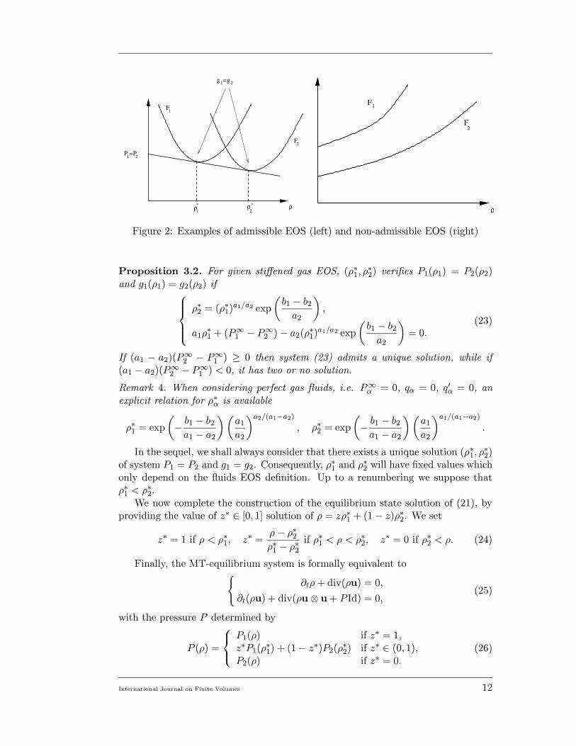
g1 = g2 if and only if D1(ρ∗1) and D2(ρ∗2) have the same slope and same F -intercept,namely D1(ρ∗1) = D2(ρ∗2). This geometrical construction of ρ∗α, called the bi-tangentcondition, is illustrated in the figure 2.

We now consider the case of stiffened gas EOS. For such fluids, the EOS aregiven by

Pα = aαρα − P∞α , gα = bα + aα log(ρα), (22)

where the constants aα and bα are related to the constant flow temperature T asfollows

aα(T ) = (γα − 1)cvαT,

bα(T ) = qα +[γαcvα − q′α + (γα − 1)cvα log

[(γα − 1)cvα

]− cvα log T

]T.

Parameters γα > 1, P∞α ≥ 0, cvα > 0, qα and q′α being constant for each fluidα = 1, 2. For this particular EOS case, the bi-tangent condition is equivalent to thefollowing analytical condition. Let us finally note that for a stiffened gas c2

α = aα,α = 1, 2.


** ρ

F1

F2

ρ ρ2

P1=P2

1

g1 g= 2

ρ

F1

F2

Figure 2: Examples of admissible EOS (left) and non-admissible EOS (right)

Proposition 3.2. For given stiffened gas EOS, (ρ∗1, ρ∗2) verifies P1(ρ1) = P2(ρ2)

and g1(ρ1) = g2(ρ2) if

ρ∗2 = (ρ∗1)a1/a2 exp

(b1 − b2a2

),

a1ρ∗1 + (P∞1 − P∞2 )− a2(ρ∗1)a1/a2 exp

(b1 − b2a2

)= 0.

(23)

If (a1 − a2)(P∞2 − P∞1 ) ≥ 0 then system (23) admits a unique solution, while if(a1 − a2)(P∞2 − P∞1 ) < 0, it has two or no solution.

Remark 4. When considering perfect gas fluids, i.e. P∞α = 0, qα = 0, q′α = 0, anexplicit relation for ρ∗α is available

ρ∗1 = exp

(− b1 − b2a1 − a2

)(a1

a2

)a2/(a1−a2)

, ρ∗2 = exp

(− b1 − b2a1 − a2

)(a1

a2

)a1/(a1−a2)

.

In the sequel, we shall always consider that there exists a unique solution (ρ∗1, ρ∗2)

of system P1 = P2 and g1 = g2. Consequently, ρ∗1 and ρ∗2 will have fixed values whichonly depend on the fluids EOS definition. Up to a renumbering we suppose thatρ∗1 < ρ∗2.

We now complete the construction of the equilibrium state solution of (21), byproviding the value of z∗ ∈ [0, 1] solution of ρ = zρ∗1 + (1− z)ρ∗2. We set

z∗ = 1 if ρ < ρ∗1, z∗ =ρ− ρ∗2ρ∗1 − ρ∗2

if ρ∗1 < ρ < ρ∗2, z∗ = 0 if ρ∗2 < ρ. (24)

Finally, the MT-equilibrium system is formally equivalent to

∂tρ+ div(ρu) = 0,

∂t(ρu) + div(ρu⊗ u + P Id) = 0,(25)

with the pressure P determined by

P (ρ) =

P1(ρ) if z∗ = 1,z∗P1(ρ∗1) + (1− z∗)P2(ρ∗2) if z∗ ∈ (0, 1),P2(ρ) if z∗ = 0.

(26)


The resulting pressure law ρ 7→ P (ρ) is continuously differentiable with theexception of points ρ∗1 and ρ∗2 where it is only continuous (see figure 3.3 for theprofile of ρ 7→ P (ρ)). System (25) has a structure close to the isothermal Eulerequations, however, the system is only weakly hyperbolic. Indeed, for ρ /∈ ρ∗1, ρ∗2,it is possible to compute the jacobian matrix associated with the system. It possessestwo eigenvalues Λ∗1 = u−c∗ and Λ∗2 = u+c∗, where (c∗)2 = dP/dρ. While c∗ > 0 forρ /∈ [ρ∗1, ρ

∗2], in the case ρ ∈ (ρ∗1, ρ

∗2), c∗ = 0. In this case, both eigenvalues collapse

and the system looses its eigenvector basis.

P (ρ)

ρρ∗1 ρ∗2

P ∗

Hyperbolicity Loss

Figure 3: Profile of the pressure law ρ 7→ P (ρ).

A remarkable property of the resulting equilibrium system is that it complieswith an entropy convexification argument.

Proposition 3.3. Let us consider the subset E of the (ρ, F )-plane which is the unionof the function ρα 7→ ραfα(ρα) epigraphs, namely

E = (ρ, F ) ∈ (R+)2/F ≥ ρmin[f1(ρ), f2(ρ)].

Let C be the convex hull of E and let F be the function whose epigraph is C. Bydefinition F is (weakly) convex, F + ρ|u|2/2 is an entropy for the system (25) andthe pressure P in (26) is defined by P = dF/dρ− F .

This convexifcation property has been previously used within the broader contextof anisothermal flows by S. Jaouen in [16] as a design principle. The key idea wasto break down the spinodal zone in a fluid EOS by replacing it with a convexifiedsurface. In this way, the system (25)–(26) coincide with the models derived byS. Jaouen when considering isothermal flows. Let us also underline that the loss ofhyperbolicity is a pathology that seems only to affect the present isothermal models.

Remark 5. Within the present formalism, the equilibrium pressure law given by (26)when z∗ /∈ 0, 1 can be interpreted as the saturation pressure and depends solely onthe temperature T .


Remark 6. The solution of the Riemann problem for the MT-equilibrium system maynot be unique in the class of weak entropic solutions. In this sense, the system isnot well-posed in this class of solutions.

3.4 Connection with the Van der Waals Equation of States

In this section we explore the connection between the equilibrium states of the Vander Waals EOS and the MT-equilibrium system.

The volumic free energy for the Van der Waals reads

F (ρ) = ρf(ρ) = −aρ2 −RTρ ln

(1

ρ− b),

which gives the well-known Van der Waals pressure law

P (ρ) = ρ2 df

dρ(ρ) =

ρRT

1− bρ − aρ2,

where R, a and b are positive constants. As we only consider isothermal transfor-mations, we did not use the temperature T as a variable but as a parameter of theEOS. We suppose that the temperature is below the critical temperature, namelyT < 8a

27Rb . Figure 4 depicts the behavior of ρ 7→ P (ρ) and ρ 7→ F (ρ) for such tem-perature values. Let us recall the definition of the Maxwell points below the critical

P (ρ)

ρρ∗1 ρ∗2

P ∗

F (ρ)

ρρ∗1 ρ∗2

P ∗

Figure 4: Graph of the (P, ρ) and (F, ρ) isotherms for the Van der Waals EOS.

temperature: there exist two values ρ∗1 and ρ∗2 such that

g(ρ∗1) = g(ρ∗2), P (ρ∗1) = P (ρ∗2) = P ∗. (27)

Two interpretations of relation (27) are available. In the (P, ρ)-plane, equation (27)corresponds with the definition of the Maxwell points: (ρ∗1, P

∗) and (ρ∗2, P∗) cut the

graph of the (P, ρ) isotherm such that both hatched areas displayed on figure 4 areequal. Another equivalent standpoint uses the graph of the isotherm in the (F, ρ)-plane: the line defined by (ρ∗1, P

∗) and (ρ∗1, P∗) is the bi-tangent to the isotherm


graph. As seen previously, the slope of the bi-tangent line is g(ρ∗1) = g(ρ∗2) and itsF -intercept is P ∗.

The definition of the equilibria can also be expressed within both (P, ρ) and(F, ρ) framework. In the (P, ρ)-plane, the equilibrium points of the Van der Waalsequation verifies the relation ρ 7→ P eq(ρ), where

P eq(ρ) =

P (ρ), if ρ < ρ∗1,

P ∗, if ρ∗1 ≤ ρ ≤ ρ∗2,

P (ρ), if ρ∗2 < ρ.

In the F -v plane, the equilibrium points comply with the EOS ρ 7→ F eq(ρ), wherethe graph of ρ 7→ F eq(ρ) is the convex hull of the graph of ρ 7→ F (ρ).

Proposition 3.4. There exist two EOS ρα 7→ Fα(ρα), α = 1, 2 such that the MT-equilibrium system associated with the fluids governed by F1 and F2 is the equilibriumsystem of the Van der Waals EOS. Moreover, there is an infinity of possible choicesfor F1 and F2.

Proof. Let Cvdw be the graph of ρ 7→ F (ρ) where F is the free energy of Van derWaals. Consider a smooth strictly convex curve C1 (resp. C2) that coincides withρ 7→ F (ρ) for ρ < ρ∗1 (resp. ρ∗2 < ρ) and that is tangential to C1 (resp. C2) atρ = ρ∗1 (resp. ρ = ρ∗2) as depicted on figure 5. It is straightforward that union of C1

epigraph and C2 epigraph has the same convex hull as Cvdw. Therefore if Cα is thegraph of ρα 7→ Fα(ρα), α = 1, 2 then the MT-equilibrium system associated with F1

and F2 is the equilibrium system associated with the Van der Waals EOS.

F (ρ)

ρρ∗1 ρ∗2

P ∗

F1(ρ1) F2(ρ2)

Figure 5: Graph of two EOS in the (F, ρ)-plane whose MT-equilibrium is the equi-librium of the Van der Waals EOS.


4 Numerical Treatment

From now on, we shall suppose that both fluids are governed by a stiffened gas EOS.The numerical schemes are presented within a 1D framework. For the 2D tests weimplemented a classical directionnal splitting strategy.

Consider i ∈ Z, n ∈ N and let ∆x > 0 and ∆t > 0 be the space and timesteps. Recalling that W = (ρ1z1, ρ2z2, ρu)T , we note Wn

i and zni the finite volumeapproximation of W and z in the cell i at the instant tn = n∆t

Wni '

1

∆x

∫ (i+1/2)∆x

(i−1/2)∆xW(x, tn)dx, zni '

1

∆x

∫ (i+1/2)∆x

(i−1/2)∆xz(x, tn)dx.

The numerical strategy we adopt here is a classical two-step scheme which consistsin a first convective step thanks to a discretization of the source terms free relaxedsystem (15)

Wn+1/2i = Wn

i −∆t

∆x

[Gi+1/2(Wn, zn)−Gi−1/2(Wn, zn)

],

zn+1/2i = zni −

∆t

∆xHi(W

n, zn),

(28)

followed by a projection (or relaxation) step onto the equilibrium states

(Wn+1, zn+1) = Π(Wn+1/2, zn+1/2).

The choice of a non-conservative scheme for z complies with the numerical techniquespresented in [1, 2] for the five-equation model. This choice is also a simple meanthat ensures a discrete maximum principle for z during the advection step.

Remark 7. The discretization of the equation for z is absolutely not necessary forsolving the MT-equilibrium system as the projection step destroys the value zn+1/2.Nevertheless we chose to keep this keep this evolution step from zn to zn+1/2 in thepresent algorithm. This allows to switch from the MT-equilibrium system to theM-equilibrium system depending on wether the projection step is performed or not.

4.1 Numerical Scheme for the Convective Part

Following a similar approach as in [2] and [9], we shall use an upwind scheme foroperator Hi(W

n, zn) while the numerical flux operator Gi+1/2 will be derived usinga Roe-type linearization.

4.1.1 Roe-Type Linearization

Recall that V = (W, z) and let us consider two constant states VL and VR, respec-tively on the left and right of the interface i+ 1/2. Let us recall classical notations :for any vector or scalar a quantity, we note

∆a = aR − aL, a =

√ρLaL +

√ρRaR√

ρL +√ρR

, a =

√ρLaR +

√ρRaL√

ρL +√ρR

.


Our goal here is to define the vector R such that

Gi+1/2(Wn, zn) = G(Wni , z

ni ,W

ni+1, z

ni+1),

G(VL,VR) =1

2

z1ρ1uz2ρ2uρu2 + P

L

+1

2

z1ρ1uz2ρ2uρu2 + P

R

− 1

2R(VL,VR).

Let us consider a matrix A∗ that we choose to be some average of A(VL) andA(VR) the values of the Jacobian matrix defined by relation (16) in section 3.1 takenat the states VL and VR. The form of A∗ ensures that this matrix is diagonalizable.

Additionnaly, as for a classical Roe linearization we require A∗ to satisfy a jumprelation (see [21]). Since, system (15) is not in conservative form, one cannot imposethe usual jump condition. Rather, A∗ must satisfy a weak form of the Roe jumpcondition

∆(ρ1z1u)∆(ρ2z2u)

∆(ρu2 + P )u∗∆z

= A∗(VR −VL). (29)

The relation (29) is based on the Rankine-Hugoniot relations that are available forthe system (15) without source terms. The jump relation (29) is expressed in termsof the quasi-conservative variables V = (W, z) instead of the conservative variables(W, ρz) which should be used in a classical Roe scheme approach. Let us once againemphasizes that the jump relation used in (29) in unambiguously valid as z and ucannot jump simultaneously.

We have the following property for the parameters that define A∗.

Proposition 4.1. If one defines u∗, y∗α and ρ∗ by

u∗ = u, ρ∗ = ρ and y∗α = yα, (30)

and if there exists (cα)2 and M∗ such that the following discrete jump condition isverified

∆P =∑

α

(c2α)∗∆(ραzα) +M∗∆z, (31)

then the Roe matrix A∗ defined with the above parameters verifies the jump condition(29).

4.1.2 Numerical scheme

We now assume that we have a matrix A∗ whose coefficient complies with the con-dition of proposition 4.1. We shall note (Λ∗j )j=1,...,4, (r∗j )j=1,...,4 and (l∗j )j=1,...,4 re-spectively the eigenvalues of A∗, the corresponding right and left eigenvectors basisdefined by relations (17)–(18). Recall that the usual Roe numerical flux is given by|A∗|∆V. In our case, we only keep its first three components denoted by R(VL,VR).More precisely, for 1 ≤ k ≤ 3, the kth component of R is given by

Rk = (|A∗|∆V)k =4∑

j=1

|Λ∗j |β∗j (r∗j )k k = 1, 2, 3, (32)


where β∗j = l∗j ·∆V.The jump relation (31) along with some basic algebra provide that β∗j verify

β∗1 =1

2(c∗)2

[∆P − ρc∗∆u

],

β∗2 =1

(c∗)2

[−y1∆P + (c∗)2∆(ρ1z1)

],

β∗3 =1

(c∗)2

[−y2∆P + (c∗)2∆(ρ2z2)

],

β∗4 =1

2(c∗)2

[∆P + ρc∗∆u

].

Using the above formulas for (β∗k)k=1,...4 allows to compute R(VL,VR) withoutcomputing M∗ nor (c2

α)∗, α = 1, 2. The sole value of (c∗)2 is needed. Within theframework of stiffened gas EOS we chose

(c∗)2 = y1a1 + y1a2.

The numerical scheme related to the convective part before the projection onequilibrium manifolds finally reads

Wn+1/2i = Wn

i −∆t

∆x

(Gni+1/2 −Gn

i−1/2

),

where the numerical flux Gni+1/2 is given by

Gi+1/2 =1

2

ρ1z1

ρ2z2

ρu2 + P

i+1

+1

2

ρ1z1

ρ2z2

ρu2 + P

i

− 1

2R(Vi+1,Vi).

The color function z is advected using the following upwind scheme

zn+1/2i = zni −

∆t

2∆x

[(uni − |u|ni )(zni+1 − zni ) + (uni + |u|ni )(zni − zni−1)

].

Remark 8. The Roe-type solver described in this section can capture solutions thatviolate the entropy condition, e.g.when the solution comes across a sonic point. Inorder to remedy this flaw, we used the classical entropy fix introduced in [13] thatconsists in substituting Q(Λ∗j , υ) for |Λ∗j | in formula (32), where υ ∈ R is a smallparameter and

Q(Λ∗j , υ) =

|Λ∗j |, if |Λ∗j | > υ,12

((Λ∗j )

2/υ + υ), if |Λ∗j | ≤ υ.

Let us underline that for the numerical tests we performed the above fix did not seemmandatory as it did not appear to carry a great influence with the numerical solution.


4.2 Relaxation Towards the M-Equilibrium (M-scheme)

For the M-equilibrium system, we suppose the parameter λ to be finite but very large.We formally set κ = +∞ which imposes that the equilibrium value is retrieved bysolving equation (19). With the stiffened gas assumption, we are able to give anexplicit expression for z∗, namely

z∗ =β

1 + β,

β =−(a2m2−a1m1−P∞2 +P∞1

)+

√(a2m2−a1m1−P∞2 +P∞1

)2+4a1a2m1m2

2a2m2.

(33)

Remark 9. We emphasize once more that projection onto the M-equilibrium maybe irrelevant when m1m2 = 0, depending on the EOS used for the fluid 1 and thefluid 2. The relation (33) gives a good insight into this ambiguity. If one considerstwo EOS such that P∞2 6= P∞1 then for m1 = 0 we have β 6= 0 which implies thatz∗ 6= 0. On the contrary, if one considers P∞2 = P∞1 = 0, then limm1→0β = 0 andlimm2→0β = 0.

Using a splitting operator, we integrate over [0,∆t] the following ODE system

∂tm1 = λ[g2(ρ2)− g1(ρ1)

], ∂tρ = 0, ∂t(ρu) = 0, (34)

with intial condition (W, z)(0) = (W, z)n+1/2i .

For stability and maximum principle purpose, instead of a direct numerical inte-gration of system (34), we seek for an approximate ODE system that allows explicitintegration. In order to do so we scale parameter λ by setting λ = m1m2λ, whereλ is a supposed large constant parameter. Then, we also freeze the (g2 − g1) termin its value (g2 − g1)n+1/2 evaluated at (W, z)n+1/2. We obtain the simplified ODEsystem

∂t(m1) = λm1(ρn+1/2i −m1)(g2 − g1)

n+1/2i , ∂tρ = 0, ∂t(ρu) = 0, (35)

which can be solved explicitly

m1(t) =ρn+1/2i[

ρn+1/2i /(m1)

n+1/2i − 1

]exp

[− λtρn+1/2

i (g2 − g1)n+1/2i

]+ 1

, (36)

andρ(t) = ρ

n+1/2i , u(t) = u

n+1/2i .

Let us notice that the above relation ensures m1(t) ∈ [0, ρ(t)] for all t > 0. Wenow complete the source integration step by setting

ρn+1i = ρ

n+1/2i , un+1

i = un+1/2i , (m1)n+1

i = m1(∆t), (m2)n+1i = ρn+1

i − (m1)n+1i .

Finally, we update z by remapping z onto the M-equilibrium states by usingexpression (33) with Wn+1.


4.3 Relaxation Towards the MT-equilibrium (MT-scheme)

We now suppose the existence of densities ρ∗1 < ρ∗2 solution of P1 = P2 and g1 = g2

known either explicitly in the case of perfect gases (see remark 4), either by solving(23) with an iterative algorithm for the case of stiffened gas. The intermediarysolution (Wn+1/2, zn+1/2) obtained after the convective step (28) is projected ontothe MT-equilibrium states using relation (24). This leads to

zn+1i =

1 if ρn+1/2i < ρ∗1,

ρn+1/2i − ρ∗2ρ∗1 − ρ∗2

if ρ∗1 < ρn+1/2i < ρ∗2,

0 if ρ∗2 < ρn+1/2i ,

for zn+1i ,

(m1,m2

)n+1

i=

(ρn+1/2i , 0

)if ρ

n+1/2i < ρ∗1,

(ρ∗1z

n+1i , ρ∗2(1− zn+1

i ))

if ρ∗1 < ρn+1/2i < ρ∗2,

(0, ρ

n+1/2i

)if ρ∗2 < ρ

n+1/2i ,

for partial densities of both phases and ρn+1i = ρ

n+1/2i , un+1

i = un+1/2i .

5 Numerical Results

5.1 Pure Interface Advection

We consider a one dimensional advection problem: a 1 m long domain contains liq-uid and vapor initially separated by an interface located at x = 0.5 m. Both fluidsα = 1, 2 are governed by a stiffened EOS (see relation 22) where the parameters(aα, bα, P

∞α )α=1,2, of the fluids are given in table 1. Velocities of both fluids are

fixed at u = 100 m.s−1 and densities are chosen on each side of the interface suchthat the pressure is constant in the whole domain, namely ρ = ρ∗1 = 1.0 kg.m−3 onthe left (fluid 1) and ρ = ρ∗2 = 2.0 kg.m−3 on the right (fluid 2).

fluid 1 (left) fluid 2 (right)

P∞ (Pa) 0 0.5

a (Pa.kg−1.m3) 1.5 1.0

b (J) ln(2) 0

Table 1: Fluids parameters for the pure advection test.

Boundary conditions are constant states on both side of the domain which is dis-cretized over 100 cells. Figure 6 displays the solution obtained with the MT-scheme


(dots) and the solution obtained with the Roe scheme applied to the system (15)without source terms (solid lines).

Although this test is a simple Riemann problem which does not involve phasechange but purely kinetic effects, we emphasize the fact that the MT-equilibriumsystem we deal with does not match the classical hyperbolic well-posedness criteria.However, we can check that the MT-scheme seems to capture the same advectedprofile as the Roe scheme applied to (15) without source terms. Indeed, we obtainthe same propagation speed without any pressure nor velocity perturbations.

0

0.2

0.4

0.6

0.8

1

0 0.1 0.2 0.3 0.4 0.5 0.6 0.7 0.8 0.9 1 1.485

1.49

1.495

1.5

1.505

1.51

1.515

0 0.1 0.2 0.3 0.4 0.5 0.6 0.7 0.8 0.9 1

z Pressure

0.8

1

1.2

1.4

1.6

1.8

2

0 0.1 0.2 0.3 0.4 0.5 0.6 0.7 0.8 0.9 1 99

99.5

100

100.5

101

0 0.1 0.2 0.3 0.4 0.5 0.6 0.7 0.8 0.9 1

Density Velocity

Figure 6: Time evolution of the MT-equilibrium solution computed with MT-scheme(dots) and the solution of the pure convective part of the system (15) computed witha Roe scheme (solid lines); t varies from t = 0 s to t = 4 ms.


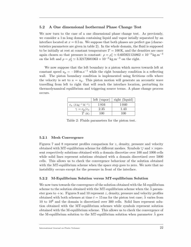
5.2 A One dimensional Isothermal Phase Change Test

We now turn to the case of a one dimensional phase change test. As previously,we consider a 1 m long domain containing liquid and vapor intially separated by aninterface located at x = 0.5 m. We suppose that both phases are perfect gas (charac-teristics parameters are given in table 2). In the whole domain, the fluid is supposedto be initially at rest at constant temperature T = 100 K, and the densities are onceagain chosen so that pressure is constant: ρ = ρ∗1 ' 0.605921124862 × 10−3 kg.m−3

on the left and ρ = ρ∗2 ' 3.32172681063 × 10−3 kg.m−3 on the right.

We now suppose that the left boundary is a piston which moves towards left atconstant speed up = −100 m.s−1 while the right boundary condition is a reflectingwall. The piston boundary condition is implemented using fictitious cells wherethe velocity is set to u = up. This piston motion will generate an accoustic wavetravelling from left to right that will reach the interface location, perturbing itsthermodynamical equilibrium and triggering source terms. A phase change processoccurs.

left (vapor) right (liquid)

cv (J.kg−1.K−1) 1 816 1 040

γ = cp/cv 2.35 1.43

T (K) 100 100

Table 2: Fluids parameters for the piston test.

5.2.1 Mesh Convergence

Figures 7 and 8 represent profiles comparison for z, density, pressure and velocityobtained with MT-equilibrium scheme for different meshes. Symbols5 and × repre-sent respectively solutions obtained with a domain discretize over 100 and 1000 cellswhile solid lines represent solutions obtained with a domain discretized over 5000cells. This allows us to check the convergence behaviour of the solution obtainedwith the MT-equilibrium scheme when the space step goes to zero. We note that noinstability occurs except for the pressure in front of the interface.

5.2.2 M-Equilibrium Solution versus MT-equilibrium Solution

We now turn towards the convergence of the solution obtained with the M-equilibriumscheme to the solution obtained with the MT-equilibrium scheme when the λ param-eter goes to +∞. Figures 9 and 10 represent z, density, pressure and velocity profilesobtained with both schemes at time t = 15 ms for the piston test case; λ varies from10 to 106 and the domain is discretized over 300 cells. Solid lines represent solu-tion obtained with the MT-equilibrium schemes while symbols represent solutionobtained with the M-equilibrium scheme. This allows us to check the convergence ofthe M-equilibrium solution to the MT-equilibrium solution when parameter λ goes


z Density

0

0.2

0.4

0.6

0.8

1

0 0.1 0.2 0.3 0.4 0.5 0.6 0.7 0.8 0.9 1 0.0005

0.001

0.0015

0.002

0.0025

0.003

0.0035

0 0.1 0.2 0.3 0.4 0.5 0.6 0.7 0.8 0.9 1

t = 4.90 ms t = 4.90 ms

0

0.2

0.4

0.6

0.8

1

0 0.1 0.2 0.3 0.4 0.5 0.6 0.7 0.8 0.9 1 0.0005

0.001

0.0015

0.002

0.0025

0.003

0.0035

0 0.1 0.2 0.3 0.4 0.5 0.6 0.7 0.8 0.9 1

t = 9.65 ms t = 9.65 ms

0

0.2

0.4

0.6

0.8

1

0 0.1 0.2 0.3 0.4 0.5 0.6 0.7 0.8 0.9 1 0.0005

0.001

0.0015

0.002

0.0025

0.003

0.0035

0 0.1 0.2 0.3 0.4 0.5 0.6 0.7 0.8 0.9 1

t = 15 ms t = 15 ms

Figure 7: z and density profiles comparison between solutions for different mesh sizesobtained with the MT-equilibrium scheme; symbols 5 and × represent respectivelysolutions obtained with a domain discretize over 100 and 1000 cells while solid linesrepresent solutions obtained with a domain discretized over 5000 cells.


Pressure Velocity

139

140

141

142

143

144

145

146

147

148

149

0 0.1 0.2 0.3 0.4 0.5 0.6 0.7 0.8 0.9 1-100

-90

-80

-70

-60

-50

-40

-30

-20

-10

0

10

0 0.1 0.2 0.3 0.4 0.5 0.6 0.7 0.8 0.9 1

t = 4.90 ms t = 4.90 ms

141

142

143

144

145

146

147

148

149

0 0.1 0.2 0.3 0.4 0.5 0.6 0.7 0.8 0.9 1-120

-100

-80

-60

-40

-20

0

0 0.1 0.2 0.3 0.4 0.5 0.6 0.7 0.8 0.9 1

t = 9.65 ms t = 9.65 ms

141

142

143

144

145

146

147

148

149

0 0.1 0.2 0.3 0.4 0.5 0.6 0.7 0.8 0.9 1-120

-100

-80

-60

-40

-20

0

0 0.1 0.2 0.3 0.4 0.5 0.6 0.7 0.8 0.9 1

t = 15 ms t = 15 ms

Figure 8: Pressure and velocity profiles comparison between solutions for differentmesh sizes obtained with the MT-equilibrium; symbols 5 and × represent respec-tively solutions obtained with a domain discretize over 100 and 1000 cells while solidlines represent solutions obtained with a domain discretized over 5000 cells.


to +∞.

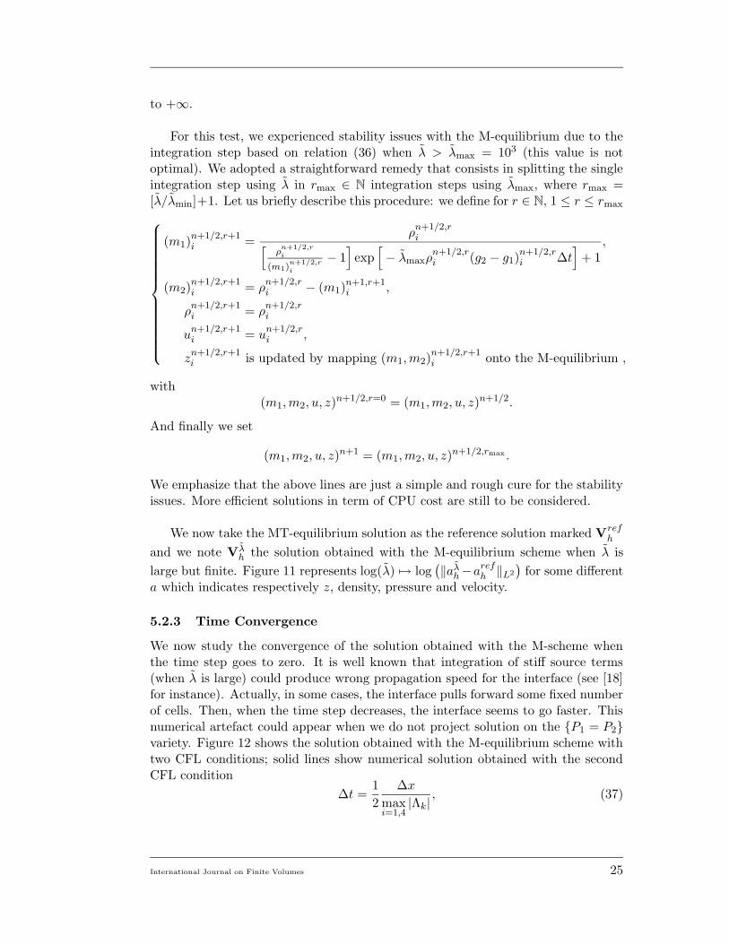
For this test, we experienced stability issues with the M-equilibrium due to theintegration step based on relation (36) when λ > λmax = 103 (this value is notoptimal). We adopted a straightforward remedy that consists in splitting the singleintegration step using λ in rmax ∈ N integration steps using λmax, where rmax =[λ/λmin]+1. Let us briefly describe this procedure: we define for r ∈ N, 1 ≤ r ≤ rmax

(m1)n+1/2,r+1i =

ρn+1/2,ri[

ρn+1/2,ri

(m1)n+1/2,ri

− 1]

exp[− λmaxρ

n+1/2,ri (g2 − g1)

n+1/2,ri ∆t

]+ 1

,

(m2)n+1/2,r+1i = ρ

n+1/2,ri − (m1)n+1,r+1

i ,

ρn+1/2,r+1i = ρ

n+1/2,ri

un+1/2,r+1i = u

n+1/2,ri ,

zn+1/2,r+1i is updated by mapping (m1,m2)

n+1/2,r+1i onto the M-equilibrium ,

with(m1,m2, u, z)n+1/2,r=0 = (m1,m2, u, z)n+1/2.

And finally we set

(m1,m2, u, z)n+1 = (m1,m2, u, z)n+1/2,rmax .

We emphasize that the above lines are just a simple and rough cure for the stabilityissues. More efficient solutions in term of CPU cost are still to be considered.

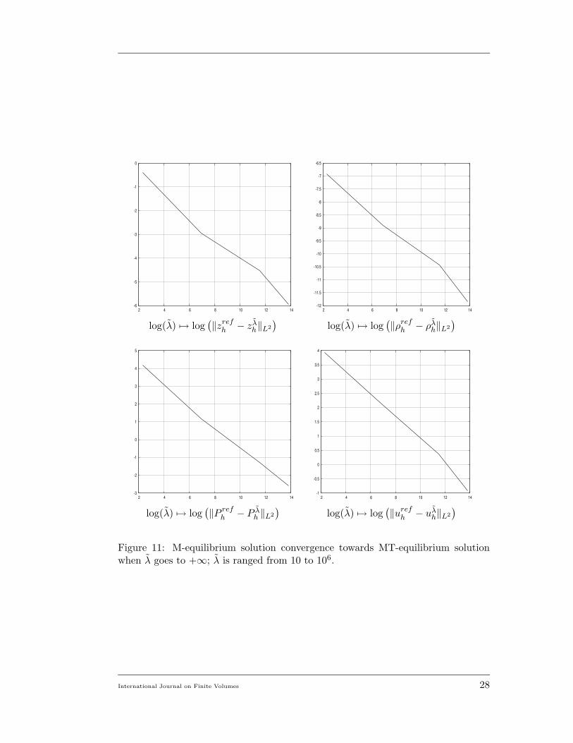
We now take the MT-equilibrium solution as the reference solution marked Vrefh

and we note Vλh the solution obtained with the M-equilibrium scheme when λ is

large but finite. Figure 11 represents log(λ) 7→ log(‖aλh−a

refh ‖L2

)for some different

a which indicates respectively z, density, pressure and velocity.

5.2.3 Time Convergence

We now study the convergence of the solution obtained with the M-scheme whenthe time step goes to zero. It is well known that integration of stiff source terms(when λ is large) could produce wrong propagation speed for the interface (see [18]for instance). Actually, in some cases, the interface pulls forward some fixed numberof cells. Then, when the time step decreases, the interface seems to go faster. Thisnumerical artefact could appear when we do not project solution on the P1 = P2variety. Figure 12 shows the solution obtained with the M-equilibrium scheme withtwo CFL conditions; solid lines show numerical solution obtained with the secondCFL condition

∆t =1

2

∆x

maxi=1,4

|Λk|, (37)


z Density

0

0.2

0.4

0.6

0.8

1

0 0.1 0.2 0.3 0.4 0.5 0.6 0.7 0.8 0.9 1 0.0005

0.001

0.0015

0.002

0.0025

0.003

0.0035

0 0.1 0.2 0.3 0.4 0.5 0.6 0.7 0.8 0.9 1

λ = 10 λ = 10

0

0.2

0.4

0.6

0.8

1

0 0.1 0.2 0.3 0.4 0.5 0.6 0.7 0.8 0.9 1 0.0005

0.001

0.0015

0.002

0.0025

0.003

0.0035

0 0.1 0.2 0.3 0.4 0.5 0.6 0.7 0.8 0.9 1

λ = 103 λ = 103

0

0.2

0.4

0.6

0.8

1

0 0.1 0.2 0.3 0.4 0.5 0.6 0.7 0.8 0.9 1 0.0005

0.001

0.0015

0.002

0.0025

0.003

0.0035

0 0.1 0.2 0.3 0.4 0.5 0.6 0.7 0.8 0.9 1

λ = 106 λ = 106

Figure 9: z and density profiles comparison between M-equilibrium solution andMT-equilibrium solution; t = 15 ms, λ is ranged from 10 to 106.


Pressure Velocity

20

40

60

80

100

120

140

160

0 0.1 0.2 0.3 0.4 0.5 0.6 0.7 0.8 0.9 1-120

-100

-80

-60

-40

-20

0

0 0.1 0.2 0.3 0.4 0.5 0.6 0.7 0.8 0.9 1

λ = 10 λ = 10

136

138

140

142

144

146

148

150

0 0.1 0.2 0.3 0.4 0.5 0.6 0.7 0.8 0.9 1-120

-100

-80

-60

-40

-20

0

0 0.1 0.2 0.3 0.4 0.5 0.6 0.7 0.8 0.9 1

λ = 103 λ = 103

141

142

143

144

145

146

147

148

149

0 0.1 0.2 0.3 0.4 0.5 0.6 0.7 0.8 0.9 1-120

-100

-80

-60

-40

-20

0

20

0 0.1 0.2 0.3 0.4 0.5 0.6 0.7 0.8 0.9 1

λ = 106 λ = 106

Figure 10: pressure and velocity profiles comparison between M-equilibrium solutionand MT-equilibrium solution; t = 15 ms, λ is ranged from 10 to 106.


-6

-5

-4

-3

-2

-1

0

2 4 6 8 10 12 14-12

-11.5

-11

-10.5

-10

-9.5

-9

-8.5

-8

-7.5

-7

-6.5

2 4 6 8 10 12 14

log(λ) 7→ log(‖zrefh − zλh‖L2

)log(λ) 7→ log

(‖ρrefh − ρλh‖L2

)

-3

-2

-1

0

1

2

3

4

5

2 4 6 8 10 12 14-1

-0.5

0

0.5

1

1.5

2

2.5

3

3.5

4

2 4 6 8 10 12 14

log(λ) 7→ log(‖P refh − P λh ‖L2

)log(λ) 7→ log

(‖urefh − uλh‖L2

)

Figure 11: M-equilibrium solution convergence towards MT-equilibrium solutionwhen λ goes to +∞; λ is ranged from 10 to 106.


while5 symbols show numerical solution obtained with the following CFL condition

∆t =1

200

∆x

maxi=1,4

|Λk|. (38)

The domain is discretized over 100 cells and λ is fixed at 106. This show us that thenumerical solution, and consequently the velocity of the interface, does not dependon the time step.

0

0.2

0.4

0.6

0.8

1

0 0.1 0.2 0.3 0.4 0.5 0.6 0.7 0.8 0.9 1 0.0005

0.001

0.0015

0.002

0.0025

0.003

0.0035

0 0.1 0.2 0.3 0.4 0.5 0.6 0.7 0.8 0.9 1

z density

141

142

143

144

145

146

147

148

149

0 0.1 0.2 0.3 0.4 0.5 0.6 0.7 0.8 0.9 1-120

-100

-80

-60

-40

-20

0

20

0 0.1 0.2 0.3 0.4 0.5 0.6 0.7 0.8 0.9 1

pressure velocity

Figure 12: z, density, pressure and velocity profiles comparison for solutions obtainedwith the M-equilibrium scheme; the time step is given by CFL condition (37) (solidlines) and (38) (5 symbols).


5.3 Compression of a Gas Bubble

We consider a 1 m long square domain discretized over 100×100 cells mesh. A vaporbubble is surrounded by liquid in the center of the domain. The radius is initiallyr = 25 cm. The EOS used are stiffened gas type whose coefficients are given in table1. The temperature is fixed to T = 600 K and densities are given by ρ∗1 ' 35.5 k.m−3

for the vapor and ρ∗2 ' 686.25 kg.m−3 for the liquid.

We suppose the left boundary be a piston moves toward right at constant speedup = 100 m.s−1. The other boundary conditions are reflecting wall. Figure 13 showsthe z profile obtained with the MT-scheme (on the left) and the z profile obtainedwith the homogeneous system (on the right) at various instants. We notice thatwith the MT-scheme, a phase change occurs and the vapor bubble liquefies while forthe off-equilibrium system (15) without source terms, the bubble is just compressed.

5.4 Depression of Two Liquid Drops

We again consider a 1 m long square domain discretized over 100 × 100 cells wheretwo drops of dodecan liquid are surrouned by dodecan vapor. Both equations ofstate are stiffened gas type whose coefficients are given in table 3. Temperature isfixed at 600 K and as previously, densities of liquid and vapor are choosen such thatphases are at mecanic and thermodynamic equilibrium, namely ρ∗1 = 12.08 kg.m−3

for the vapor and ρ∗2 = 458.62 kg.m−3 for the liquid.

liquid vapor

cv (J.kg−1.K−1) 1077.7 1956.45

γ = Cp/Cv 2.35 1.025

P∞ (Pa) 4.108 0

q (kJ.kg−1) −755.269 −237.547

q′ (kJ.kg−1.K−1) 0 −24.485

Table 3: Fluid parameters for liquid and vapor dodecan.

On the left of the domain, a depression is simulated by imposing a constantvelocity up = −100 m.s−1 in fictitious cells. Other boundary conditions are reflectivewalls. Figures 14, 15, 16 and 17 show respectively z, density, pressure and velocityin the x-direction profiles for time varying from t = 2 ms to t = 32 ms. This allowsus to show the vaporization of liquid bubbles due to the depression.

6 Conclusion

We have presented in this paper a dynamical phase-change model for compress-ible flows. The physical model derivation has been detailed. We have proposeda numerical Finite-Volume based discretization approach which complies with theentropy balance of the model. This feature is important as uniqueness fails in the


general class of entropy solutions for the equilibrium MT-equilibrium system. In thisway, while ill-posedness for this model is still an open issue, we can conjecture thatthe approximate solution obtained with our approach complies with the dissipativestructures of the relaxed model.

The present modelling and numerical approach extend to the anisothermal frame-work with little efforts. It has been recently achieved in [5]. Even stronger connec-tions with the seminal work of Jaouen [16] and Barberon & Helluy [3, 14], which arenot yet clarified, are to be expected.

References

[1] G. Allaire, S. Clerc, and S. Kokh. A five-equation model for the numericalsimulation of interfaces in two-phase flows. C. R. Acad. Sci. Paris, Serie I,t. 331:pp. 1017–1022, 2000.

[2] G. Allaire, S. Clerc, and S. Kokh. A five-equation model for the simulation ofinterfaces between compressible fluids. J. Comp. Phys., 181:pp. 577–616, 2002.

[3] T. Barberon and Ph. Helluy. Finite volume simulation of cavitating flows.Computers and Fluids, 34(7):pp. 832—858, 2005.

[4] A. Bedford. Hamilton’s principle in continuum mechanics. Research Notes inMathematics, 1985.

[5] F. Caro. Modelisation et simulation numerique des transitions de phase liquide-vapeur. PhD thesis, Ecole Polytechnique, 2004.

[6] F. Caro, F. Coquel, D. Jamet, and S. Kokh. DINMOD: A diffuse interfacemodel for two-phase flows modelling. In S. Cordier, T. Goudon, M. Gutnic,and E. Sonnendrucker, editors, Numerical methods for hyperbolic and kineticproblems, IRMA lecture in mathematics and theoretical physics (Proceedings ofthe CEMRACS 2003), 2005.

[7] F. Caro, F. Coquel, D. Jamet, and S. Kokh. Phase change simulation forisothermal compressible two-phase flows. In AIAA Comp. Fluid Dynamics,number AIAA-2005-4697, 2005.

[8] P. Casal and H. Gouin. A representation of liquid-vapor interfaces by usingfluids of second gradient. Annales de physique, Colloque num. 2, 13, 1988.

[9] G. Chanteperdrix, Ph. Villedieu, and J.P. Vila. A compressible model for sepa-rated two-phase flows computations. In Proceedings os ASME Fluid Eng. Div.Summer Meeting 2002, 2002. Paper 3114.

[10] J.M. Delhaye, M. Giot, and M.L. Riethmuller. Thermohydraulics of Two-PhaseSystems for Industrial Design and Nuclear Engineering. Hemisphere PublishingCorporation, 1981.


[11] S. Gavrilyuk and H. Gouin. A new form of governing equations of fluids arisingfrom Hamilton’s principle. International Journal of Engineering Science, 37,1999.

[12] S. Gavrilyuk and R. Saurel. Mathematical and numerical modeling of two-phasecompressible flows with micro-inertia. J. Comp. Phys., 175:326–360, 2002.

[13] A. Harten and J.M. Hyman. Self adjusting grid methods for one-dimensionalhyperbolic conservation laws. J. Comp. Phys., 50:pp. 235–269, 1983.

[14] Ph. Helluy. Simulation numerique des ecoulements multiphasiques : de latheorie aux applications.(these d’habilitation). Technical report, 2005.

[15] D. Jamet, O. Lebaigue, N. Coutris, and J.M. Delhaye. The second gradientmethod for the direct numerical simulation of liquid-vapor flows with phasechange. J. Comp. Phys., 169:624–651, 2001.

[16] S. Jaouen. Etude mathematique et numerique de stabilite pour des modeleshydrodynamiques avec transition de phase. PhD thesis, Univ. Paris 6, 2001.

[17] F. Lagoutiere. Modelisation mathematique et resolution numerique de problemesde fluides a plusieurs constituants. PhD thesis, Univ. Paris 6, 2002.

[18] R. J. LeVeque and H. C. Yee. A study of numerical methods for hyperbolicconservation laws with stiff source terms. J. Comp. Phys, 86:187–210, 1990.

[19] J. Massoni, R. Saurel, B. Nkonga, and R. Abgrall. Proposition de methodeset modeles euleriens pour les problemes a interfaces entre fluides compressiblesen presence de transfert de chaleur: Some models and eulerian methods forinterface problems between compressible fluids with heat transfer. Int. J. ofHeat and Mass Transfer, 45(6):pp. 1287–1307, 2002.

[20] O. Le Metayer. Modelisation et resolution de la propagation de fronts per-meables: application aux fronts d’evaporation et de detonation. PhD thesis,Universite de Provence (Aix-Marseille 1), 2003.

[21] P.L. Roe. Approximate Riemann solvers, parameter vectors and differenceschemes. J. Comp. Phys., 43:pp. 357–372, 1981.

[22] R. Salmon. Hamiltonian fluid mechanics. Ann. Rev. Fluid Mech., (20):pp. 225–256, 1988.

[23] L. Truskinovsky. Kinks versus shocks. In R. Fosdick and al., editors, Shock in-duced transitions and phase structures in general media. Springer Verlag, Berlin,1991.


With phase change Without phase change

t = 0 s t = 0 s

t = 0.54 ms t = 0.54 ms

t = 1.08 ms t = 1.08 ms

Figure 13: z profile obtained with the MT-scheme on the bottom and z profileobtained with the homogeneous system on the top; t varies from t = 0 s to t =1.08 ms.


t = 2 ms t = 8 ms

t = 14 ms t = 20 ms

t = 26 ms t = 32 ms

Figure 14: z profile obtained with the MT-equilibrium scheme; t varies from 2 ms to32 ms.


t = 2 ms t = 8 ms

t = 14 ms t = 20 ms

t = 26 ms t = 32 ms

Figure 15: Density profile obtained with the MT-equilibrium scheme; t varies from2 ms to 32 ms.


t = 2 ms t = 8 ms

t = 14 ms t = 20 ms

t = 26 ms t = 32 ms

Figure 16: Pressure profile obtained with the MT-equilibrium scheme; t varies from2 ms to 32 ms.


t = 2 ms t = 8 ms

t = 14 ms t = 20 ms

t = 26 ms t = 32 ms

Figure 17: Velocity in the x-direction profile obtained with the MT-equilibriumscheme; t varies from 2 ms to 32 ms.


a simple finite-volume method for compressible isothermal

Documents