a simple elasto-plastic model for soils … web page/nsf workshop 2005/presentations... · a simple...

A simple elastoplastic model for soils and soft rocks

Baltimore, November 3rd 2005

A SIMPLE ELASTO-PLASTIC MODEL FOR SOILS AND SOFT ROCKS

byRoberto Nova

Milan University of Technology



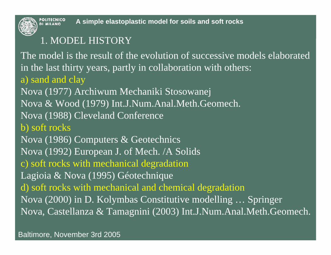
1. MODEL HISTORYThe model is the result of the evolution of successive models elaborated in the last thirty years, partly in collaboration with others:a) sand and clayNova (1977) Archiwum Mechaniki StosowanejNova & Wood (1979) Int.J.Num.Anal.Meth.Geomech.Nova (1988) Cleveland Conferenceb) soft rocksNova (1986) Computers & GeotechnicsNova (1992) European J. of Mech. /A Solidsc) soft rocks with mechanical degradationLagioia & Nova (1995) Géotechniqued) soft rocks with mechanical and chemical degradationNova (2000) in D. Kolymbas Constitutive modelling … SpringerNova, Castellanza & Tamagnini (2003) Int.J.Num.Anal.Meth.Geomech.



2. MODEL STRUCTURE FOR UNCEMENTED SOILS

Simple elastic plastic strain-hardening model (as Cam Clay):

a) plastic potential gb) yield function fc) hardening rule

d) elastic law (for unloading-reloading)



Plastic potential 3 299( 3) ln ( 1) 04c

pg J Jp η ηγ γ γ′

≡ − − + − =

2 3; ; ;ij

ijpij ij ij ij ik ki

ij

sg J Jp η ηε η η η η η η

σ∂

= Λ ≡ ≡ ≡′∂

&

Deviatoric plane‘Triaxial’ (axisymmetric) plane

'p

q Mη =

2

3 2

92 33

M

M Mγ −=

+ −



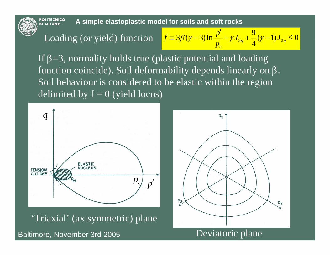
Loading (or yield) function 3 293 ( 3) ln ( 1) 04c

pf J Jp η ηβ γ γ γ′

≡ − − + − ≤

If β=3, normality holds true (plastic potential and loading function coincide). Soil deformability depends linearly on β.Soil behaviour is considered to be elastic within the region delimited by f = 0 (yield locus)

‘Triaxial’ (axisymmetric) planeDeviatoric plane

p′

q

cp



{ }1/ 2 1/3( ) ( )

13

p p p p p pcc rs rs rs rs rs st tr

p

hk hk rs rs

pp e e e e eB

e

ε δ ξ ψ

ε ε δ

= + +

= −

&& & & & & &

& &&

Hardening rule:

Bp is the plastic volumetric logarithmic complianceξ and ψ control dilatancy in triaxial compression and extension

''

eij e ij ij

pB Lp

ε δ η= +&

& &Hypoelastic relationship:

pc is the isotropic preconsolidation pressure, controlling the size of the elastic domain

Be is the elastic volumetric logarithmic complianceL is a shear stiffness proportionality constant (G increasing with p’)



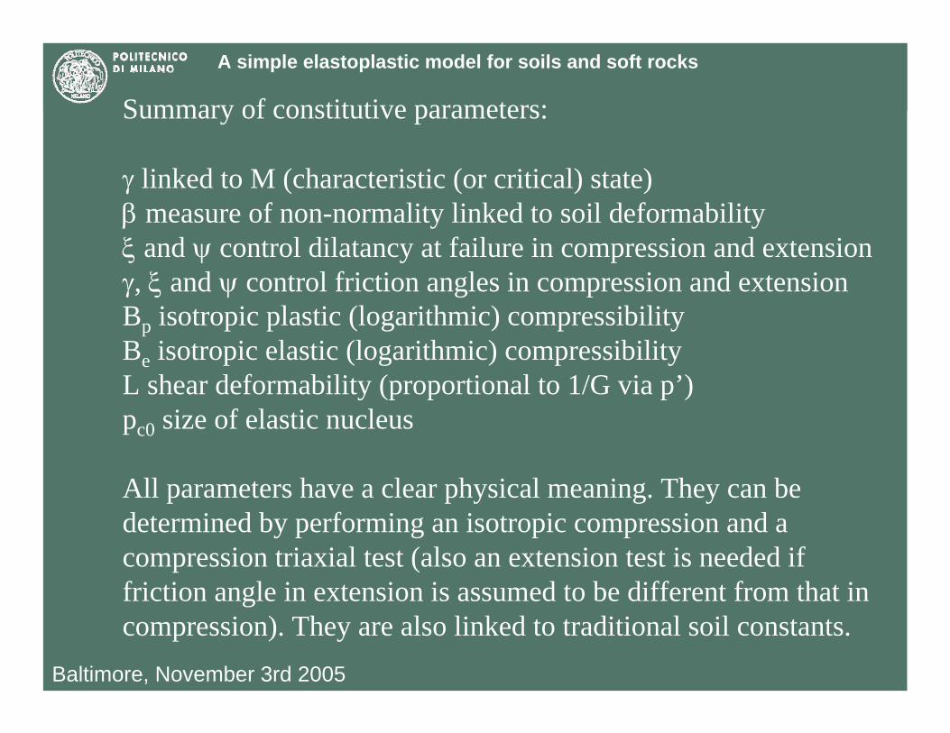
Summary of constitutive parameters:

γ linked to M (characteristic (or critical) state)β measure of non-normality linked to soil deformabilityξ and ψ control dilatancy at failure in compression and extensionγ, ξ and ψ control friction angles in compression and extensionBp isotropic plastic (logarithmic) compressibilityBe isotropic elastic (logarithmic) compressibilityL shear deformability (proportional to 1/G via p’)pc0 size of elastic nucleus

All parameters have a clear physical meaning. They can be determined by performing an isotropic compression and a compression triaxial test (also an extension test is needed if friction angle in extension is assumed to be different from that in compression). They are also linked to traditional soil constants.



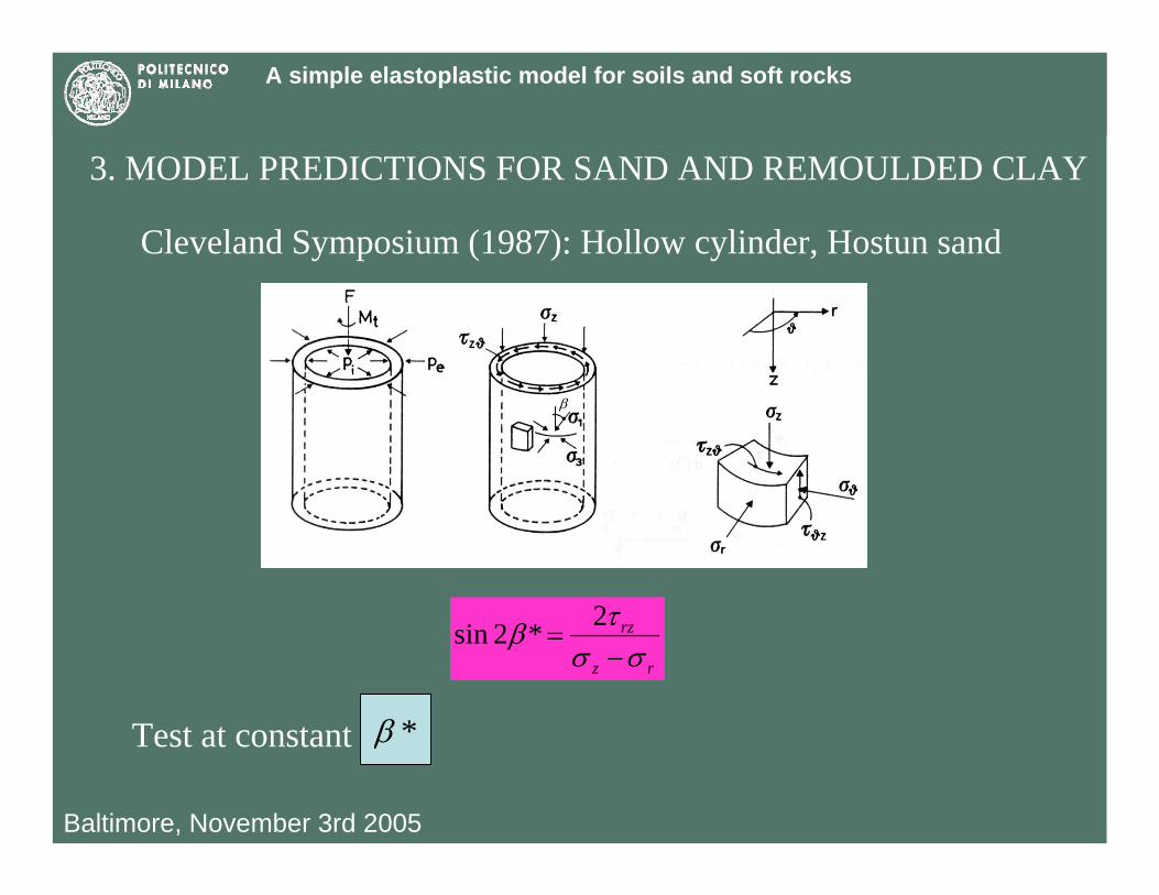
Cleveland Symposium (1987): Hollow cylinder, Hostun sand

2sin 2 * rz

z r

τβσ σ

=−

3. MODEL PREDICTIONS FOR SAND AND REMOULDED CLAY

β

Test at constant *β



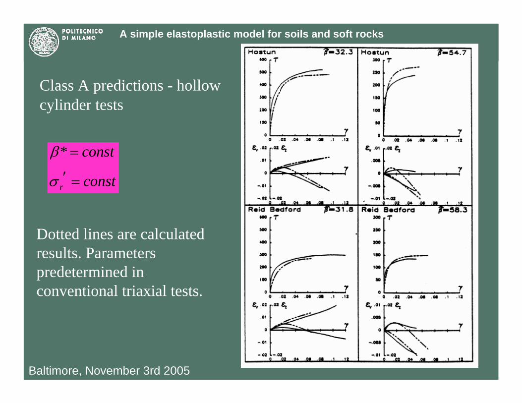
Class A predictions - hollow cylinder tests

*

r

const

const

β

σ

=

′ =

Dotted lines are calculated results. Parameters predetermined in conventional triaxial tests.



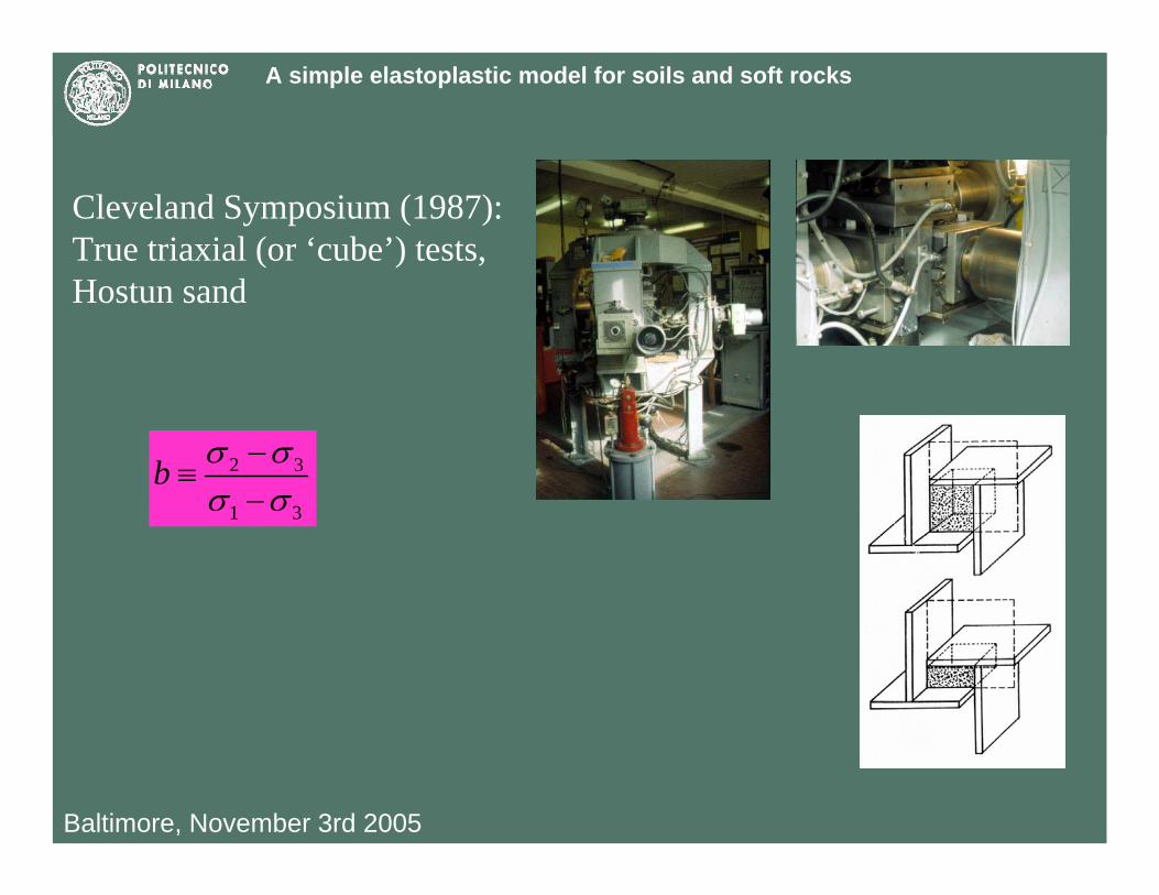
2 3

1 3

b σ σσ σ

−≡

−

Cleveland Symposium (1987): True triaxial (or ‘cube’) tests, Hostun sand



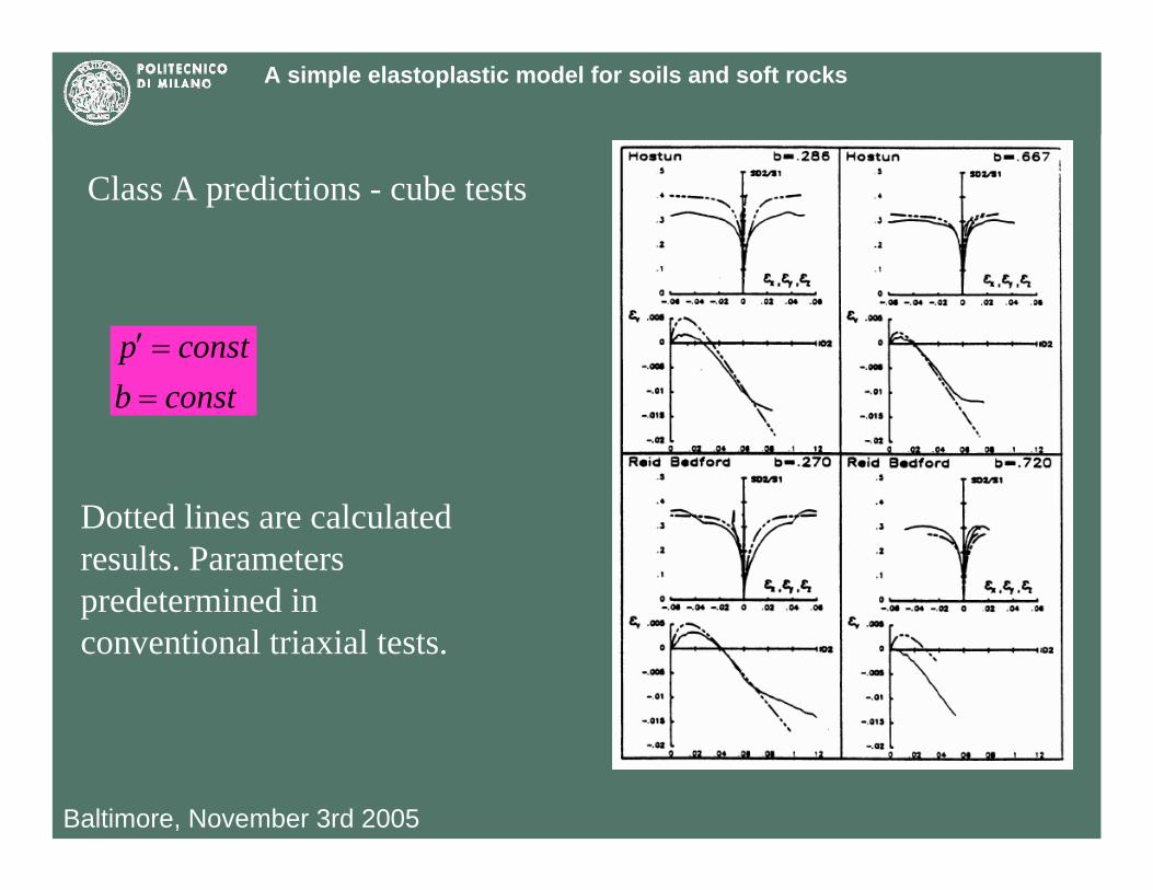
Class A predictions - cube tests

p constb const′ ==

Dotted lines are calculated results. Parameters predetermined in conventional triaxial tests.



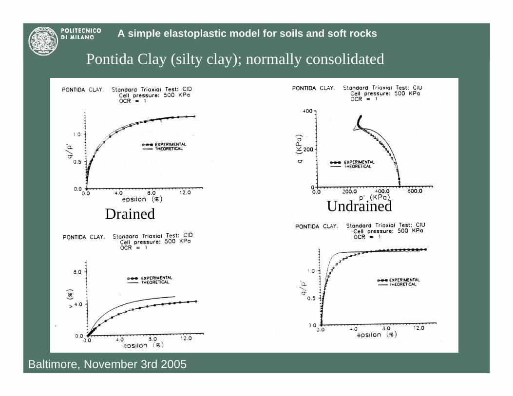
Pontida Clay (silty clay); normally consolidated

Drained Undrained



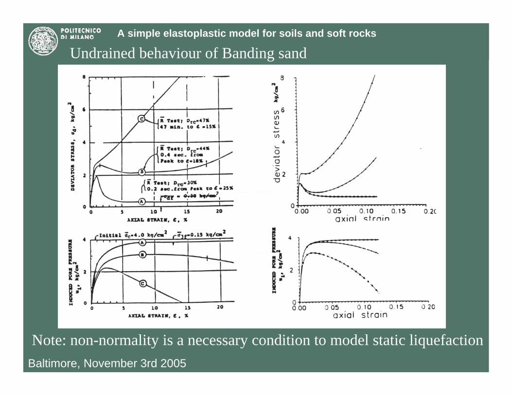
Undrained behaviour of Banding sand

Note: non-normality is a necessary condition to model static liquefaction



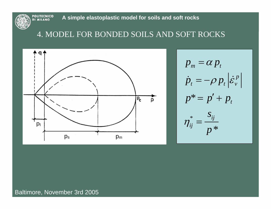
4. MODEL FOR BONDED SOILS AND SOFT ROCKS

pt

pmps

*

*

*

m t

pt t v

t

ijij

p p

p p

p p psp

α

ρ ε

η

=

= −

′= +

=

&&



Natural calcarenite: isotropic compression



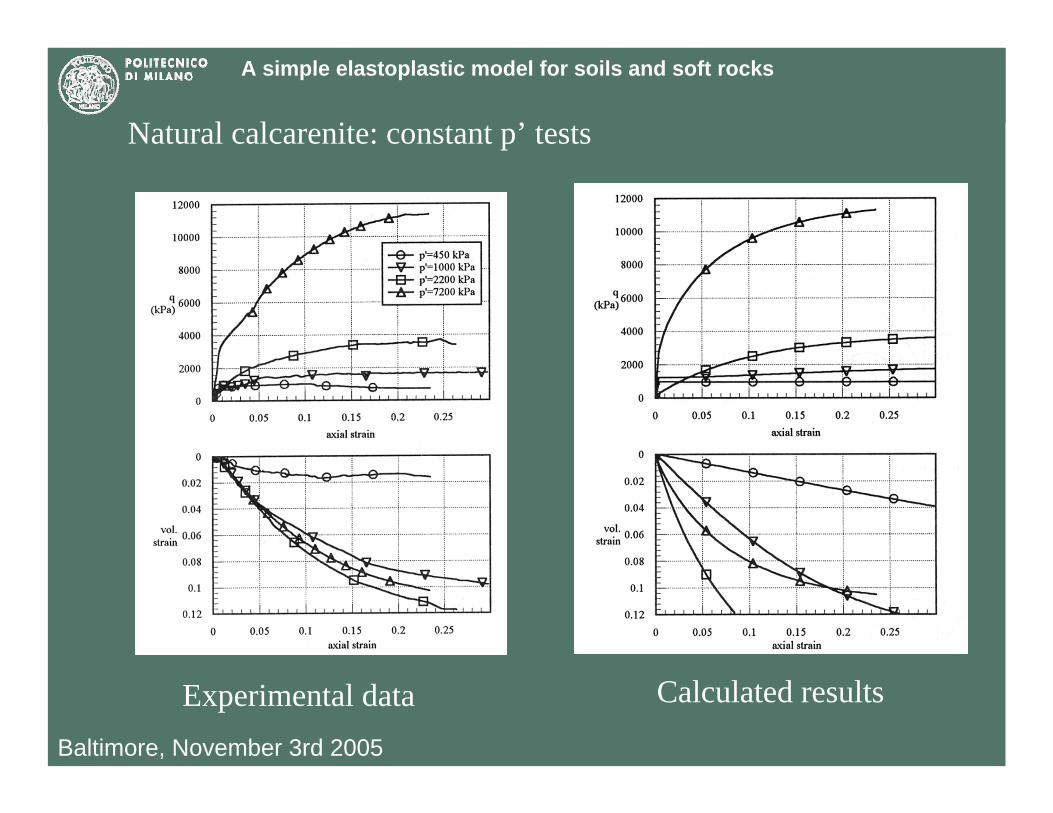
Natural calcarenite: constant p’ tests

Experimental data Calculated results



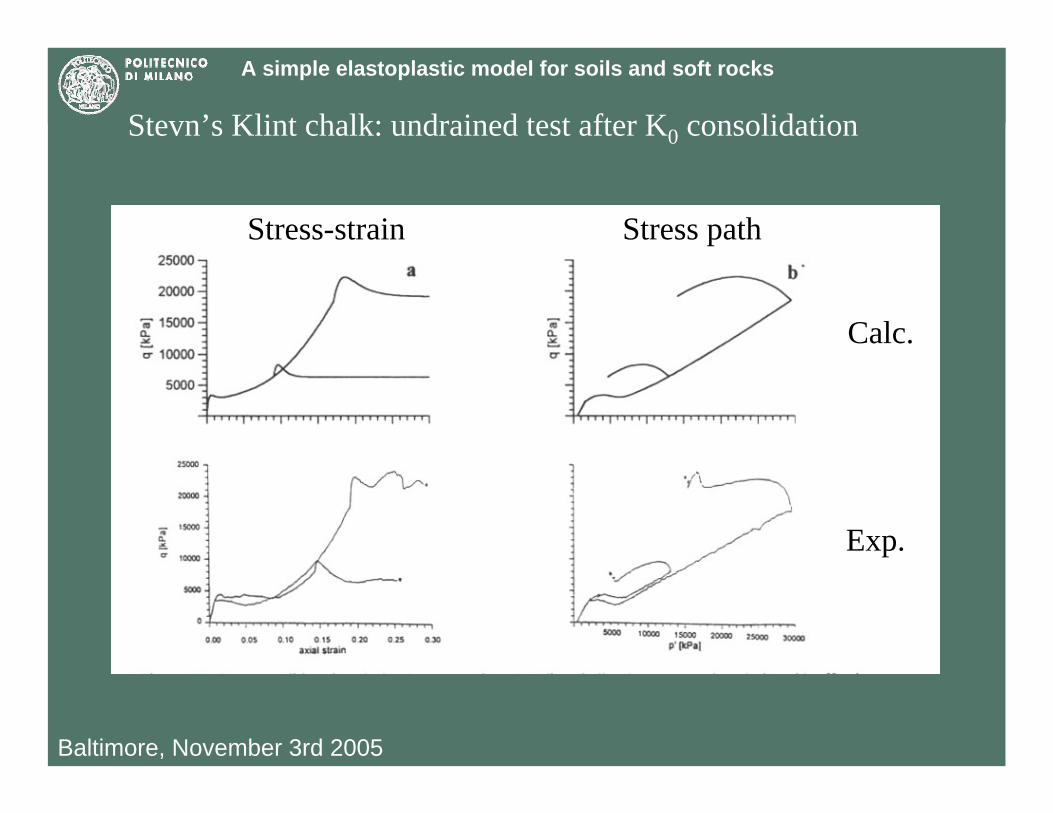
Stevn’s Klint chalk: undrained test after K0 consolidation

Exp.

Calc.

Stress-strain Stress path



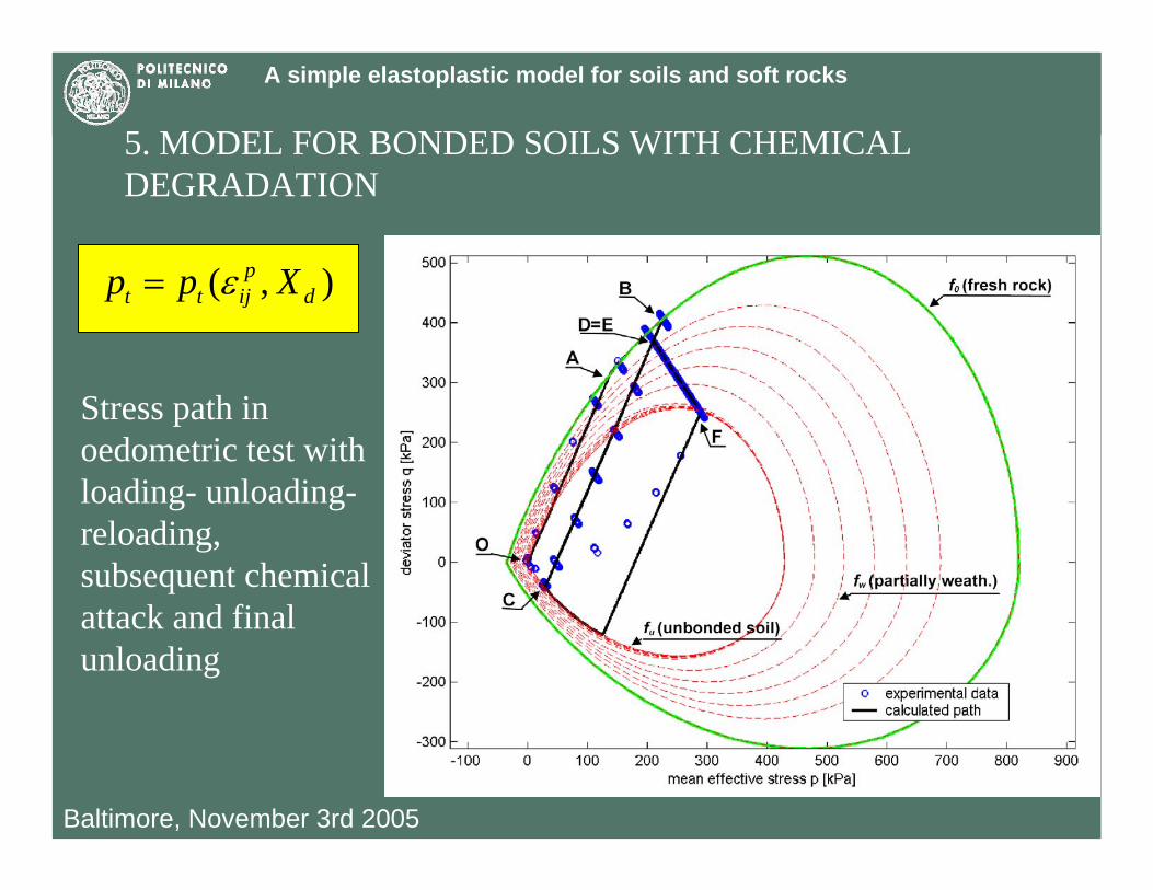
5. MODEL FOR BONDED SOILS WITH CHEMICAL DEGRADATION

( , )pt t ij dp p Xε=

Stress path in oedometric test with loading- unloading-reloading, subsequent chemical attack and final unloading



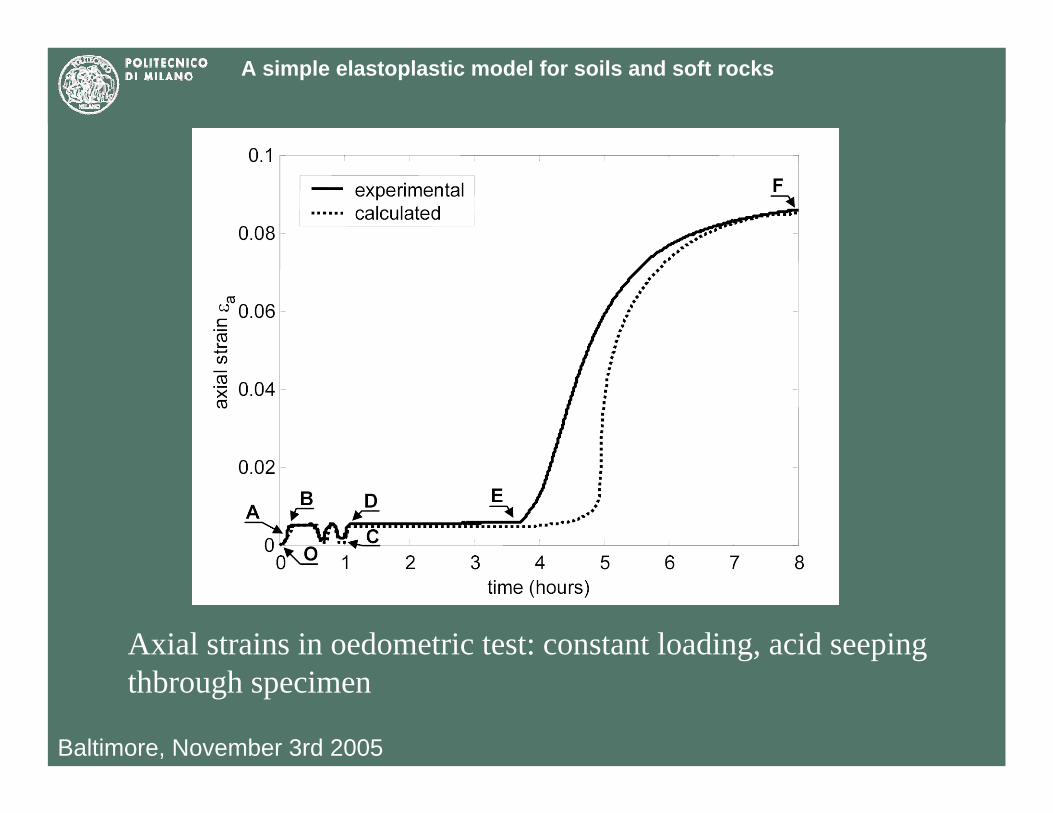
Axial strains in oedometric test: constant loading, acid seeping thbrough specimen



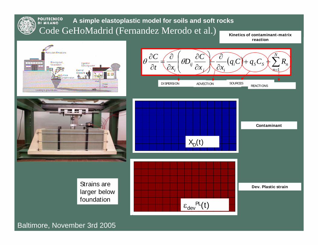
Kinetics of contaminant-matrix reaction

Dev. Plastic strain

Contaminant

XD(t)

εdevPL(t)

Strains are larger belowfoundation

( ) ∑=

++∂∂

−⎟⎟⎠

⎞⎜⎜⎝

⎛

∂∂

∂∂

=∂∂ N

nnSSi

ijij

i

RCqCqxx

CDxt

C1

θθ

DISPERSION ADVECTION SOURCESREACTIONS

Code GeHoMadrid (Fernandez Merodo et al.)



Problems of practical interest can be solved by means of numerical methods with advanced constitutive models. Academicians must convince practicioners that the solutions obtained in this way are better than those one can obtain with ‘simple’ constitutive models.

Select a number of problems, compare the solution one can obtainwith an advanced constitutive model and that one can obtain withe.g. Drucker Prager and show which is the qualitative enhancement by using the former.

WORKSHOPS ON B.V.P.? Explore the role of:dilatancy (non normality) occurrence of plastic strains prior to failure (‘anisotropy’)cementation and degradationsoftening, shear banding and other types of instabilities (e.g. static liquefaction)



Academicians must also show that the number of parameters and their determination is not an obstacle for practical applications

Academicians should guarantee that their numerical solutions areobjective. More research is needed for the numerical treatment of softening, shear banding and other types of instability. Creep effects must be explicitly taken into account.

Progress in science (knowledge) implies that more and more concepts should be studied and understood by ‘students’. Therefore academicians must:

- give a sound theoretical basis even at the undergraduate level- disseminate extra moenia recent ideas- try to confront themselves with practical problems



Students and practitioners MUST STUDY



PANEL DISCUSSION

The static problem is characterised by:

• 3 different materials (loose sand, soft clay, stiff clay)• Clay consolidation (negative friction on piles) • Three-dimensional loading conditions (piles)• Rotation of principal stresses



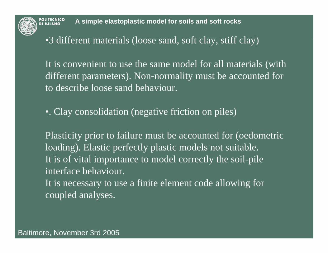
•3 different materials (loose sand, soft clay, stiff clay)

It is convenient to use the same model for all materials (with different parameters). Non-normality must be accounted for to describe loose sand behaviour.

•. Clay consolidation (negative friction on piles)

Plasticity prior to failure must be accounted for (oedometric loading). Elastic perfectly plastic models not suitable.It is of vital importance to model correctly the soil-pile interface behaviour.It is necessary to use a finite element code allowing for coupled analyses.



•Three-dimensional loading conditions (piles)

Drucker-Prager (and any other model with circular cross section in the deviatoric plane) is not suitable for this problem.

•Rotation of principal stresses

This item could be properly addressed only by using a constitutive model with coupled isotropic-kinematic hardening (yield function rotating with plastic strains, see e.g. di Prisco et al. (1995)). Isotropic elasto-plastic models with strain-hardening provide at least a response that depends on the incremental stress direction.



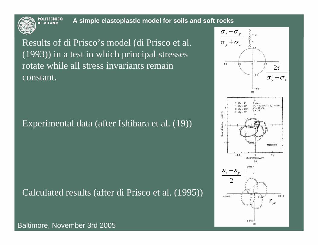
Results of di Prisco’s model (di Prisco et al. (1993)) in a test in which principal stresses rotate while all stress invariants remain constant.

Experimental data (after Ishihara et al. (19))

Calculated results (after di Prisco et al. (1995))

2

y z

τσ σ+

z y

y z

σ σσ σ

−

+

yzε

2z yε ε−

a simple elasto-plastic model for soils … web page/nsf workshop 2005/presentations... · a simple...

Documents