a short overview thomas girke december 6,...

Introduction to RA Short Overview

Thomas Girke

December 6, 2012

Introduction to R Slide 1/70

IntroductionLook and Feel of the R EnvironmentR Library DepositoriesInstallationGetting AroundBasic SyntaxData Types and SubsettingImportant UtilitiesBasic CalculationsReading and Writing External DataSome Great R FunctionsGraphics Utilities

Graphics EnvironmentsBase Graphics

Exercise: Analysis Routine

Introduction to R Slide 2/70

Outline




Introduction to R Introduction Slide 3/70

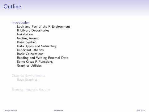
Outline




Introduction to R Introduction Look and Feel of the R Environment Slide 4/70

Why Using R?

Complete statistical package and programming language

Efficient functions and data structures for data analysis

Powerful graphics

Access to fast growing number of analysis packages

Most widely used language in bioinformatics

Is standard for data mining and biostatistical analysis

Technical advantages: free, open-source, available for all OSs

Books & Documentation

simpleR - Using R for Introductory Statistics (John Verzani, 2004) Link

Bioinformatics and Computational Biology Solutions Using R andBioconductor (Gentleman et al., 2005) Link

More on this see ”Finding Help” section in UCR Manual Link


http://cran.r-project.org/doc/contrib/Verzani-SimpleR.pdf

http://www.bioconductor.org/help/publications/books/bioinformatics-and-computational-biology-solutions/

http://manuals.bioinformatics.ucr.edu/home/R_BioCondManual#TOC-Finding-Help

What You’ll Get?

R Gui: OS X

Command-line R: Linux/OS X R Gui: Windows


RStudio: Alternative Working Environment for RNew integrated development environment (IDE) for R that workswell for beginners and developers.


Outline




Introduction to R Introduction R Library Depositories Slide 8/70

Package Depositories

CRAN (>3500 packages) general data analysis Link

Bioconductor (>600 packages) bioscience data analysis Link

Omegahat (>30 packages) programming interfaces Link

Introduction to R Introduction R Library Depositories Slide 9/70

http://cran.at.r-project.org/

http://www.bioconductor.org/

http://www.omegahat.org/

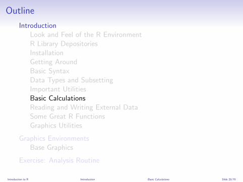
Outline




Introduction to R Introduction Installation Slide 10/70

Installation of R and Add-on Packages

Install for your operating system from:

http://cran.at.r-project.org Link

Install RStudio from:

http://www.rstudio.com/ide/download Link

Installation of CRAN Packages> install.packages(c("pkg1", "pkg2"))

> install.packages("pkg.zip", repos=NULL)

Installation of Bioconductor Packages> source("http://www.bioconductor.org/biocLite.R")

> biocLite()

> biocLite(c("pkg1", "pkg2"))

Introduction to R Introduction Installation Slide 11/70

http://cran.at.r-project.org/

http://www.rstudio.com/ide/download/

Outline




Introduction to R Introduction Getting Around Slide 12/70

Startup and Closing Behavior

Starting R

The R GUI versions, including RStudio, under Windows and Mac OS Xcan be opened by double-clicking their icons. Alternatively, one can startit by typing ’R’ in a terminal (default under Linux).

Startup/Closing Behavior

The R environment is controlled by hidden files in the startup directory:.RData, .Rhistory and .Rprofile (optional).

## Closing R

> q()

Save workspace image? [y/n/c]:

Note

When responding with ’y’, then the entire R workspace will be written tothe .RData file which can become very large. Often it is sufficient to justsave an analysis protocol in an R source file. This way one can quicklyregenerate all data sets and objects.


Getting Around

Create an object with the assignment operator <- (or =)

> object <- ...

List objects in current R session

> ls()

Return content of current working directory

> dir()

Return path of current working directory

> getwd()

Change current working directory

> setwd("/home/user")


Outline




Introduction to R Introduction Basic Syntax Slide 15/70

Basic R Syntax

General R command syntax

> object <- function_name(arguments)

> object <- object[arguments]

Finding help

> ?function_name

Load a library

> library("my_library")

Lists all functions defined by a library

> library(help="my_library")

Load library manual (PDF file)

> vignette("my_library")


Executing R Scripts

Execute an R script from within R

> source("my_script.R")

Execute an R script from command-line

Rscript my_script.R

R CMD BATCH my_script.R

R --slave < my_script.R


Outline




Introduction to R Introduction Data Types and Subsetting Slide 18/70

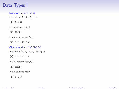
Data Types I

Numeric data: 1, 2, 3

> x <- c(1, 2, 3); x

[1] 1 2 3

> is.numeric(x)

[1] TRUE

> as.character(x)

[1] "1" "2" "3"

Character data: ”a”, ”b”, ”c”

> x <- c("1", "2", "3"); x

[1] "1" "2" "3"

> is.character(x)

[1] TRUE

> as.numeric(x)

[1] 1 2 3


Data Types II

Complex data

> c(1, "b", 3)

[1] "1" "b" "3"

Logical data

> x <- 1:10 < 5

> x

[1] TRUE TRUE TRUE TRUE FALSE FALSE FALSE FALSE FALSE FALSE

> !x

[1] FALSE FALSE FALSE FALSE TRUE TRUE TRUE TRUE TRUE TRUE

> which(x) # Returns index for the 'TRUE' values in logical vector

[1] 1 2 3 4


Data Objects: Vectors and Factors

Vectors (1D)

> myVec <- 1:10; names(myVec) <- letters[1:10]

> myVec[1:5]

a b c d e

1 2 3 4 5

> myVec[c(2,4,6,8)]

b d f h

2 4 6 8

> myVec[c("b", "d", "f")]

b d f

2 4 6

Factors (1D): vectors with grouping information

> factor(c("dog", "cat", "mouse", "dog", "dog", "cat"))

[1] dog cat mouse dog dog cat

Levels: cat dog mouse


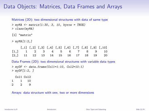
Data Objects: Matrices, Data Frames and Arrays

Matrices (2D): two dimensional structures with data of same type

> myMA <- matrix(1:30, 3, 10, byrow = TRUE)

> class(myMA)

[1] "matrix"

> myMA[1:2,]

[,1] [,2] [,3] [,4] [,5] [,6] [,7] [,8] [,9] [,10]

[1,] 1 2 3 4 5 6 7 8 9 10

[2,] 11 12 13 14 15 16 17 18 19 20

Data Frames (2D): two dimensional structures with variable data types

> myDF <- data.frame(Col1=1:10, Col2=10:1)

> myDF[1:2, ]

Col1 Col2

1 1 10

2 2 9

Arrays: data structure with one, two or more dimensions


Data Objects: Lists and Functions

Lists: containers for any object type

> myL <- list(name="Fred", wife="Mary", no.children=3, child.ages=c(4,7,9))

> myL

$name

[1] "Fred"

$wife

[1] "Mary"

$no.children

[1] 3

$child.ages

[1] 4 7 9

> myL[[4]][1:2]

[1] 4 7

Functions: piece of code

> myfct <- function(arg1, arg2, ...) {

+ function_body

+ }


General Subsetting Rules

Subsetting by positive or negative index/position numbers

> myVec <- 1:26; names(myVec) <- LETTERS

> myVec[1:4]

A B C D

1 2 3 4

Subsetting by same length logical vectors

> myLog <- myVec > 10

> myVec[myLog]

K L M N O P Q R S T U V W X Y Z

11 12 13 14 15 16 17 18 19 20 21 22 23 24 25 26

Subsetting by field names

> myVec[c("B", "K", "M")]

B K M

2 11 13

Calling a single column or list component by its name with the $ sign

> iris$Species[1:8]

[1] setosa setosa setosa setosa setosa setosa setosa setosa

Levels: setosa versicolor virginica


Outline




Introduction to R Introduction Important Utilities Slide 25/70

Combining Objects

The c function combines vectors and lists

> c(1, 2, 3)

[1] 1 2 3

> x <- 1:3; y <- 101:103

> c(x, y)

[1] 1 2 3 101 102 103

The cbind and rbind functions can be used to append columns and rows, respecively.

> ma <- cbind(x, y)

> ma

x y

[1,] 1 101

[2,] 2 102

[3,] 3 103

> rbind(ma, ma)

x y

[1,] 1 101

[2,] 2 102

[3,] 3 103

[4,] 1 101

[5,] 2 102

[6,] 3 103


Accessing Name Slots and Dimensions of Objects

Length and dimension information of objects

> length(iris$Species)

[1] 150

> dim(iris)

[1] 150 5

Accessing row and column names of 2D objects

> rownames(iris)[1:8]

[1] "1" "2" "3" "4" "5" "6" "7" "8"

> colnames(iris)

[1] "Sepal.Length" "Sepal.Width" "Petal.Length" "Petal.Width" "Species"

Return name field of vectors and lists

> names(myVec)

[1] "A" "B" "C" "D" "E" "F" "G" "H" "I" "J" "K" "L" "M" "N" "O" "P" "Q" "R" "S" "T" "U" "V" "W" "X" "Y" "Z"

> names(myL)

[1] "name" "wife" "no.children" "child.ages"


Sorting Objects

The function sort returns a vector in ascending or descending order

> sort(10:1)

[1] 1 2 3 4 5 6 7 8 9 10

The function order returns a sorting index for sorting an object

> sortindex <- order(iris[,1], decreasing = FALSE)

> sortindex[1:12]

[1] 14 9 39 43 42 4 7 23 48 3 30 12

> iris[sortindex,][1:2,]

Sepal.Length Sepal.Width Petal.Length Petal.Width Species

14 4.3 3.0 1.1 0.1 setosa

9 4.4 2.9 1.4 0.2 setosa

> sortindex <- order(-iris[,1]) # Same as decreasing=TRUE

Sorting on multiple columns

> iris[order(iris$Sepal.Length, iris$Sepal.Width),][1:2,]


14 4.3 3.0 1.1 0.1 setosa

9 4.4 2.9 1.4 0.2 setosa


Outline




Introduction to R Introduction Basic Calculations Slide 29/70

Basic Operators and Calculations

Comparison operators: ==, ! =, <, >, <=, >=

> 1==1

[1] TRUE

Logical operators: AND: &, OR: |, NOT: !

> x <- 1:10; y <- 10:1

> x > y & x > 5

[1] FALSE FALSE FALSE FALSE FALSE TRUE TRUE TRUE TRUE TRUE

Calculations: to look up math functions, see Function Index Link

> x + y

[1] 11 11 11 11 11 11 11 11 11 11

> sum(x)

[1] 55

> mean(x)

[1] 5.5

> apply(iris[1:6,1:3], 1, mean)

1 2 3 4 5 6

3.333333 3.100000 3.066667 3.066667 3.333333 3.666667

Introduction to R Introduction Basic Calculations Slide 30/70

http://cran.at.r-project.org/doc/manuals/R-intro.html#Function-and-variable-index

Outline




Introduction to R Introduction Reading and Writing External Data Slide 31/70

Reading and Writing External Data

Import data from tabular files into R

> myDF <- read.delim("myData.xls", sep="\t")

Export data from R to tabular files

> write.table(myDF, file="myfile.xls", sep="\t", quote=FALSE, col.names=NA)

Copy and paste (e.g. from Excel) into R

> ## On Windows/Linux systems:

> read.delim("clipboard")

> ## On Mac OS X systems:

> read.delim(pipe("pbpaste"))

Copy and paste from R into Excel or other programs

> ## On Windows/Linux systems:

> write.table(iris, "clipboard", sep="\t", col.names=NA, quote=F)

> ## On Mac OS X systems:

> zz <- pipe('pbcopy', 'w')

> write.table(iris, zz, sep="\t", col.names=NA, quote=F)

> close(zz)


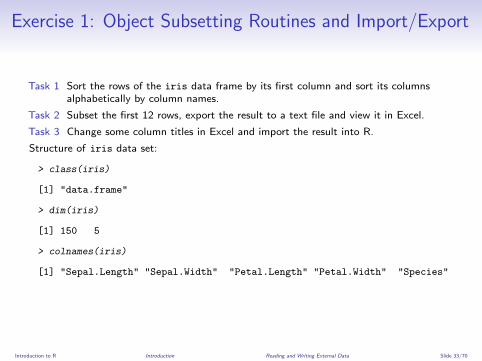
Exercise 1: Object Subsetting Routines and Import/Export

Task 1 Sort the rows of the iris data frame by its first column and sort its columnsalphabetically by column names.

Task 2 Subset the first 12 rows, export the result to a text file and view it in Excel.

Task 3 Change some column titles in Excel and import the result into R.

Structure of iris data set:

> class(iris)

[1] "data.frame"

> dim(iris)

[1] 150 5

> colnames(iris)

[1] "Sepal.Length" "Sepal.Width" "Petal.Length" "Petal.Width" "Species"


Outline




Introduction to R Introduction Some Great R Functions Slide 34/70

Some Great R Functions I

The unique() function to make vector entries unique

> length(iris$Sepal.Length)

[1] 150

> length(unique(iris$Sepal.Length))

[1] 35

The table() function counts the occurrences of entries

> table(iris$Species)

setosa versicolor virginica

50 50 50

The aggregate() function computes statistics of data aggregates

> aggregate(iris[,1:4], by=list(iris$Species), FUN=mean, na.rm=TRUE)

Group.1 Sepal.Length Sepal.Width Petal.Length Petal.Width

1 setosa 5.006 3.428 1.462 0.246

2 versicolor 5.936 2.770 4.260 1.326

3 virginica 6.588 2.974 5.552 2.026


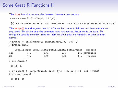
Some Great R Functions II

The %in% function returns the intersect between two vectors

> month.name %in% c("May", "July")

[1] FALSE FALSE FALSE FALSE TRUE FALSE TRUE FALSE FALSE FALSE FALSE FALSE

The merge() function joins two data frames by common field entries, here row names(by.x=0). To obtain only the common rows, change all=TRUE to all=FALSE. Tomerge on specific columns, refer to them by their position numbers or their columnnames.

> frame1 <- iris[sample(1:length(iris[,1]), 30), ]

> frame1[1:2,]


110 7.2 3.6 6.1 2.5 virginica

30 4.7 3.2 1.6 0.2 setosa

> dim(frame1)

[1] 30 5

> my_result <- merge(frame1, iris, by.x = 0, by.y = 0, all = TRUE)

> dim(my_result)

[1] 150 11


Outline




Introduction to R Introduction Graphics Utilities Slide 37/70

Graphics in R

Powerful environment for visualizing scientific data

Integrated graphics and statistics infrastructure

Publication quality graphics

Fully programmable

Highly reproducible

Full LATEX Link & Sweave Link support

Vast number of R packages with graphics utilities


http://www.latex-project.org/

http://www.stat.auckland.ac.nz/~dscott/782/Sweave-manual-20060104.pdf

Documentation on Graphics in R

General

Graphics Task Page Link

R Graph Gallery Link

R Graphical Manual Link

Paul Murrell’s book R (Grid) Graphics Link

Interactive graphics

rggobi (GGobi) Link

iplots Link

Open GL (rgl) Link


http://cran.r-project.org/web/views/Graphics.html

http://addictedtor.free.fr/graphiques/allgraph.php

http://cged.genes.nig.ac.jp/RGM2/index.php

http://www.stat.auckland.ac.nz/~paul/RGraphics/rgraphics.html

http://www.ggobi.org/

http://www.rosuda.org/iplots/

http://rgl.neoscientists.org/gallery.shtml

Graphics Environments

Viewing and saving graphics in R

On-screen graphics

postscript, pdf, svg

jpeg, png, wmf, tiff, ...

Four major graphic environments

Low-level infrastructure

R Base Graphics (low- and high-level)grid : Manual Link , Book Link

High-level infrastructure

lattice: Manual Link , Intro Link , Book Link

ggplot2: Manual Link , Intro Link , Book Link


http://www.stat.auckland.ac.nz/~paul/grid/grid.html

http://www.stat.auckland.ac.nz/~paul/RGraphics/rgraphics.html

http://lmdvr.r-forge.r-project.org

http://www.his.sunderland.ac.uk/~cs0her/Statistics/UsingLatticeGraphicsInR.htm

http://www.amazon.com/Lattice-Multivariate-Data-Visualization-Use/dp/0387759689

http://had.co.nz/ggplot2/

http://www.ling.upenn.edu/~joseff/rstudy/summer2010_ggplot2_intro.html

http://had.co.nz/ggplot2/book/

Outline




Introduction to R Graphics Environments Slide 41/70

Outline




Introduction to R Graphics Environments Base Graphics Slide 42/70

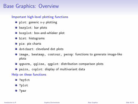
Base Graphics: Overview

Important high-level plotting functions

plot: generic x-y plotting

barplot: bar plots

boxplot: box-and-whisker plot

hist: histograms

pie: pie charts

dotchart: cleveland dot plots

image, heatmap, contour, persp: functions to generate image-likeplots

qqnorm, qqline, qqplot: distribution comparison plots

pairs, coplot: display of multivariant data

Help on these functions

?myfct

?plot

?par


Base Graphics: Preferred Input Data Objects

Matrices and data frames

Vectors

Named vectors


Scatter Plot: very basic

Sample data set for subsequent plots

> set.seed(1410)

> y <- matrix(runif(30), ncol=3, dimnames=list(letters[1:10], LETTERS[1:3]))

> plot(y[,1], y[,2])

●

●

●

●

●

●

●

●

●

●

0.2 0.4 0.6 0.8

0.2

0.4

0.6

0.8

y[, 1]

y[, 2

]


Scatter Plot: all pairs> pairs(y)

A

0.2 0.4 0.6 0.8

●

●

●

●

●

●

●

●

●

●

0.2

0.4

0.6

0.8

●

●

●

●

●

●

●

●

●

●

0.2

0.4

0.6

0.8

●

●

●

●

●

●

●

●

●

●

B ●

●

●

●

●

●

●

●

●

●

0.2 0.4 0.6 0.8

●

●

●

●

●

●

●

●

●

●

●

●

●

●

●

●

●

●

●

●

0.0 0.2 0.4 0.6 0.8 1.0

0.0

0.2

0.4

0.6

0.8

1.0

C


Scatter Plot: with labels> plot(y[,1], y[,2], pch=20, col="red", main="Symbols and Labels")

> text(y[,1]+0.03, y[,2], rownames(y))

●

●

●

●

●

●

●

●

●

●

0.2 0.4 0.6 0.8

0.2

0.4

0.6

0.8

Symbols and Labels

y[, 1]

y[, 2

]

a

b

c

d

e

f

g

h

i

j


Scatter Plots: more examples

Print instead of symbols the row names

> plot(y[,1], y[,2], type="n", main="Plot of Labels")

> text(y[,1], y[,2], rownames(y))

Usage of important plotting parameters

> grid(5, 5, lwd = 2)

> op <- par(mar=c(8,8,8,8), bg="lightblue")

> plot(y[,1], y[,2], type="p", col="red", cex.lab=1.2, cex.axis=1.2,

+ cex.main=1.2, cex.sub=1, lwd=4, pch=20, xlab="x label",

+ ylab="y label", main="My Main", sub="My Sub")

> par(op)

Important arguments

mar: specifies the margin sizes around the plotting area in order: c(bottom,

left, top, right)

col: color of symbols

pch: type of symbols, samples: example(points)

lwd: size of symbols

cex.*: control font sizes

For details see ?par


Scatter Plots: more examples

Add a regression line to a plot

> plot(y[,1], y[,2])

> myline <- lm(y[,2]~y[,1]); abline(myline, lwd=2)

> summary(myline)

Same plot as above, but on log scale

> plot(y[,1], y[,2], log="xy")

Add a mathematical expression to a plot

> plot(y[,1], y[,2]); text(y[1,1], y[1,2],

> expression(sum(frac(1,sqrt(x^2*pi)))), cex=1.3)


Exercise 2: Scatter Plots

Task 1 Generate scatter plot for first two columns in iris data frame and color dots byits Species column.

Task 2 Use the xlim/ylim arguments to set limits on the x- and y-axes so that all datapoints are restricted to the left bottom quadrant of the plot.


> class(iris)

[1] "data.frame"

> iris[1:4,]


1 5.1 3.5 1.4 0.2 setosa

2 4.9 3.0 1.4 0.2 setosa

3 4.7 3.2 1.3 0.2 setosa

4 4.6 3.1 1.5 0.2 setosa



50 50 50


Line Plot: Single Data Set

> plot(y[,1], type="l", lwd=2, col="blue")

2 4 6 8 10

0.2

0.4

0.6

0.8

Index

y[, 1

]


Line Plots: Many Data Sets> split.screen(c(1,1));

[1] 1

> plot(y[,1], ylim=c(0,1), xlab="Measurement", ylab="Intensity", type="l", lwd=2, col=1)

> for(i in 2:length(y[1,])) {

+ screen(1, new=FALSE)

+ plot(y[,i], ylim=c(0,1), type="l", lwd=2, col=i, xaxt="n", yaxt="n", ylab="",

+ xlab="", main="", bty="n")

+ }

> close.screen(all=TRUE)

2 4 6 8 10

0.0

0.2

0.4

0.6

0.8

1.0

Measurement

Inte

nsity


Bar Plot Basics> barplot(y[1:4,], ylim=c(0, max(y[1:4,])+0.3), beside=TRUE,

+ legend=letters[1:4])

> text(labels=round(as.vector(as.matrix(y[1:4,])),2), x=seq(1.5, 13, by=1)

+ +sort(rep(c(0,1,2), 4)), y=as.vector(as.matrix(y[1:4,]))+0.04)

A B C

abcd

0.0

0.2

0.4

0.6

0.8

1.0

1.2

0.27

0.53

0.93

0.14

0.47

0.31

0.050.12

0.44

0.32

0

0.41


Bar Plots with Error Bars> bar <- barplot(m <- rowMeans(y) * 10, ylim=c(0, 10))

> stdev <- sd(t(y))

> arrows(bar, m, bar, m + stdev, length=0.15, angle = 90)

a b c d e f g h i j

02

46

810


Histograms

> hist(y, freq=TRUE, breaks=10)

Histogram of y

y

Fre

quen

cy

0.0 0.2 0.4 0.6 0.8 1.0

01

23

4


Density Plots

> plot(density(y), col="red")

0.0 0.5 1.0

0.0

0.2

0.4

0.6

0.8

1.0

density.default(x = y)

N = 30 Bandwidth = 0.136

Den

sity


Pie Charts> pie(y[,1], col=rainbow(length(y[,1]), start=0.1, end=0.8), clockwise=TRUE)

> legend("topright", legend=row.names(y), cex=1.3, bty="n", pch=15, pt.cex=1.8,

+ col=rainbow(length(y[,1]), start=0.1, end=0.8), ncol=1)

a

b

c

d

ef

g

h

ij a

bcdefghij


Color Selection Utilities

Default color palette and how to change it

> palette()

[1] "black" "red" "green3" "blue" "cyan" "magenta" "yellow" "gray"

> palette(rainbow(5, start=0.1, end=0.2))

> palette()

[1] "#FF9900" "#FFBF00" "#FFE600" "#F2FF00" "#CCFF00"

> palette("default")

The gray function allows to select any type of gray shades by providing values from 0to 1

> gray(seq(0.1, 1, by= 0.2))

[1] "#1A1A1A" "#4D4D4D" "#808080" "#B3B3B3" "#E6E6E6"

Color gradients with colorpanel function from gplots library

> library(gplots)

> colorpanel(5, "darkblue", "yellow", "white")

Much more on colors in R see Earl Glynn’s color chart Link


http://research.stowers-institute.org/efg/R/Color/Chart/

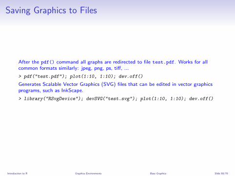
Saving Graphics to Files

After the pdf() command all graphs are redirected to file test.pdf. Works for allcommon formats similarly: jpeg, png, ps, tiff, ...

> pdf("test.pdf"); plot(1:10, 1:10); dev.off()

Generates Scalable Vector Graphics (SVG) files that can be edited in vector graphicsprograms, such as InkScape.

> library("RSvgDevice"); devSVG("test.svg"); plot(1:10, 1:10); dev.off()


Exercise 3: Bar Plots

Task 1 Calculate the mean values for the Species components of the first four columnsin the iris data set. Organize the results in a matrix where the row names arethe unique values from the iris Species column and the column names arethe same as in the first four iris columns.

Task 2 Generate two bar plots: one with stacked bars and one with horizontallyarranged bars.


> class(iris)

[1] "data.frame"

> iris[1:4,]


1 5.1 3.5 1.4 0.2 setosa

2 4.9 3.0 1.4 0.2 setosa

3 4.7 3.2 1.3 0.2 setosa

4 4.6 3.1 1.5 0.2 setosa



50 50 50


Outline




Introduction to R Exercise: Analysis Routine Slide 61/70

Analysis Routine: Overview

The following exercise introduces a variety of useful dataanalysis utilities in R.


Analysis Routine: Data Import

Step 1 To get started with this exercise, direct your R session to a dedicated workshop

directory and download into this directory the following sample tables. Then

import the files into Excel and save them as tab delimited text files.

MolecularWeight_tair7.xls Link

TargetP_analysis_tair7.xls Link

Import the tables into R

> ## Import molecular weight table

> my_mw <- read.delim(file="MolecularWeight_tair7.xls", header=T, sep="\t")

> my_mw[1:2,]

Sequence.id Molecular.Weight.Da. Residues

1 AT1G08520.1 83285 760

2 AT1G08530.1 27015 257

> ## Import subcelluar targeting table

> my_target <- read.delim(file="TargetP_analysis_tair7.xls", header=T, sep="\t")

> my_target[1:2,]

GeneName Loc cTP mTP SP other

1 AT1G08520.1 C 0.822 0.137 0.029 0.039

2 AT1G08530.1 C 0.817 0.058 0.010 0.100


http://faculty.ucr.edu/~tgirke/Documents/R_BioCond/Samples/MolecularWeight_tair7.xls

http://faculty.ucr.edu/~tgirke/Documents/R_BioCond/Samples/TargetP_analysis_tair7.xls

Analysis Routine: Merging Data Frames

Step 2 Assign uniform gene ID column titles

> colnames(my_target)[1] <- "ID"

> colnames(my_mw)[1] <- "ID"

Step 3 Merge the two tables based on common ID field

> my_mw_target <- merge(my_mw, my_target, by.x="ID", by.y="ID", all.x=T)

Step 4 Shorten one table before the merge and then remove the non-matching rows(NAs) in the merged file

> my_mw_target2a <- merge(my_mw, my_target[1:40,], by.x="ID", by.y="ID", all.x=T)

> # To remove non-matching rows, use the argument setting 'all=F'.

> my_mw_target2 <- na.omit(my_mw_target2a)

> # Removes rows containing "NAs" (non-matching rows).

Problem 1: How can the merge function in the previous step be executed so that onlythe common rows among the two data frames are returned? Prove that bothmethods - the two step version with na.omit and your method - return identicalresults.

Problem 2: Replace all NAs in the data frame my_mw_target2a with zeros.


Analysis Routine: Filtering Data

Step 5 Retrieve all records with a value of greater than 100,000 in ’MW’ column and’C’ value in ’Loc’ column (targeted to chloroplast).

> query <- my_mw_target[my_mw_target[, 2] > 100000 & my_mw_target[, 4] == "C", ]

> query[1:4, ]

ID Molecular.Weight.Da. Residues Loc cTP mTP SP other

219 AT1G02730.1 132588 1181 C 0.972 0.038 0.008 0.045

243 AT1G02890.1 136825 1252 C 0.748 0.529 0.011 0.013

281 AT1G03160.1 100732 912 C 0.871 0.235 0.011 0.007

547 AT1G05380.1 126360 1138 C 0.740 0.099 0.016 0.358

> dim(query)

[1] 170 8

Problem 3: How many protein entries in the my_mw_target data frame have a MW ofgreater then 4,000 and less then 5,000. Subset the data frame accordingly andsort it by MW to check that your result is correct.


Analysis Routine: String Substitutions

Step 6 Use a regular expression in a substitute function to generate a separate IDcolumn that lacks the gene model extensions.

> my_mw_target3 <- data.frame(loci=gsub("\\..*", "",

+ as.character(my_mw_target[,1]), perl = TRUE),

+ my_mw_target)

> my_mw_target3[1:3,1:8]

loci ID Molecular.Weight.Da. Residues Loc cTP mTP SP

1 AT1G01010 AT1G01010.1 49426 429 _ 0.10 0.090 0.075

2 AT1G01020 AT1G01020.1 28092 245 * 0.01 0.636 0.158

3 AT1G01020 AT1G01020.2 21711 191 * 0.01 0.636 0.158

Problem 4: Retrieve those rows in my_mw_target3 where the second column containsthe following identifiers: c("AT5G52930.1", "AT4G18950.1", "AT1G15385.1",

"AT4G36500.1", "AT1G67530.1"). Use the %in% function for this query. As analternative approach, assign the second column to the row index of the dataframe and then perform the same query again using the row index. Explain thedifference of the two methods.


Analysis Routine: Calculations on Data Frames

Step 7 Count the number of duplicates in the loci column with the table function andappend the result to the data frame with the cbind function.

> mycounts <- table(my_mw_target3[,1])[my_mw_target3[,1]]

> my_mw_target4 <- cbind(my_mw_target3, Freq=mycounts[as.character(my_mw_target3[,1])])

Step 8 Perform a vectorized devision of columns 3 and 4 (average AA weight perprotein)

> data.frame(my_mw_target4, avg_AA_WT=(my_mw_target4[,3] / my_mw_target4[,4]))[1:2,5:11]

Loc cTP mTP SP other Freq avg_AA_WT

1 _ 0.10 0.090 0.075 0.925 1 115.2121

2 * 0.01 0.636 0.158 0.448 2 114.6612

Step 9 Calculate for each row the mean and standard deviation across several columns

> mymean <- apply(my_mw_target4[,6:9], 1, mean)

> mystdev <- apply(my_mw_target4[,6:9], 1, sd, na.rm=TRUE)

> data.frame(my_mw_target4, mean=mymean, stdev=mystdev)[1:2,5:12]

Loc cTP mTP SP other Freq mean stdev

1 _ 0.10 0.090 0.075 0.925 1 0.2975 0.4184595

2 * 0.01 0.636 0.158 0.448 2 0.3130 0.2818912


Analysis Routine: Plotting ExampleStep 10 Generate scatter plot columns: ’MW’ and ’Residues’

> plot(my_mw_target4[1:500,3:4], col="red")

●

●●

●

●

●

●●●●

●●●●●

●●●●

●

●

●

●●●●

●●●

●●

●●

●

●●

●●●●

●●●

●

●

●

●

●●

●●●●

●

●

●●●

●

●●

●

●●

●●●

●

●●●

●●●

●

●

●●●●

●●●●●

●●

●

●●●●●

●

●

●

●

●

●

●

●

●

●●●

●

●●●

●

●

●

●

●●●●

●●●

●

●

●

●●

●

●

●●●

●●●

●

●●

●

●

●●●●●●

●●

●●

●●

●●

●●

●●

●●

●

●

●

●●●●●

●●

●●●

●

●●●

●●

●

●

●

●

●

●

●

●●●

●

●●●

●

●●●

●●

●●●●

●

●●●

●●

●

●

●●

●

●●

●●

●●

●

●●

●●

●●

●

●●●●

●●●

●●●●

●●●

●●

●

●

●

●●●●●●

●●●

●

●

●

●

●

●

●

●

●●

●

●●

●

●

●

●●●

●●

●

●●

●

●

●

●

●●●

●●

●

●●●

●

●●

●●●

●

●●

●●

●●

●

●

●

●●●

●

●

●

●●

●●●

●

●●●●

●

●

●

●

●

●●●

●●

●●

●

●

●●

●●●

●

●●

●

●●

●●

●●

●●

●

●●

●●●

●●●

●●

●●

●●

●●

●

●●

●

●

●

●

●

●●●

●●

●

●

●

●

●

●

●

●

●●

●

●

●●●

●

●

●

●●●●●●

●

●

●●

●

●

●●

●●

●

●

●

●●

●●

●

●

●●

●

●

●●●●●

●●

●

●●

●●

●

●

●●

●

●●

●●●●

●

●

●●

●●

●

●

●

●●●●

●

●●

●

●

●●

●

●

●

●●

●●●●

●

●●●●

●●●

●●

●●

●

●

●●

●

0e+00 1e+05 2e+05 3e+05 4e+05

050

015

0025

0035

00

Molecular.Weight.Da.

Res

idue

s


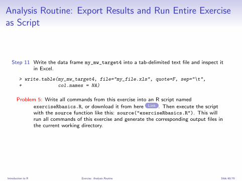
Analysis Routine: Export Results and Run Entire Exerciseas Script

Step 11 Write the data frame my_mw_target4 into a tab-delimited text file and inspect itin Excel.

> write.table(my_mw_target4, file="my_file.xls", quote=F, sep="\t",

+ col.names = NA)

Problem 5: Write all commands from this exercise into an R script named

exerciseRbasics.R, or download it from here Link . Then execute the scriptwith the source function like this: source("exerciseRbasics.R"). This willrun all commands of this exercise and generate the corresponding output files inthe current working directory.


http://faculty.ucr.edu/~tgirke/Documents/R_BioCond/My_R_Scripts/exerciseRbasics.R

Session Information

> sessionInfo()

R version 2.15.1 (2012-06-22)

Platform: x86_64-unknown-linux-gnu (64-bit)

locale:

[1] C

attached base packages:

[1] stats graphics utils datasets grDevices methods base

loaded via a namespace (and not attached):

[1] tools_2.15.1
