a short introduction on wavelet transformation and … · a short introduction on wavelet...
TRANSCRIPT
A short introduction on Wavelet Transformation
and applications in Electric DrivesDamian Giaouris BEng, BSc, PG Cert, MSc, PhD
Senior Lecturer in Control of Electrical Systems
Electrical Power Research Group
School of Electrical and Electronic Engineering,
Merz Court,
Newcastle University,
Newcastle Upon Tyne,
NE1 7RU,
United Kingdom
https://www.staff.ncl.ac.uk/damian.giaouris/
TUM – Jan 2016
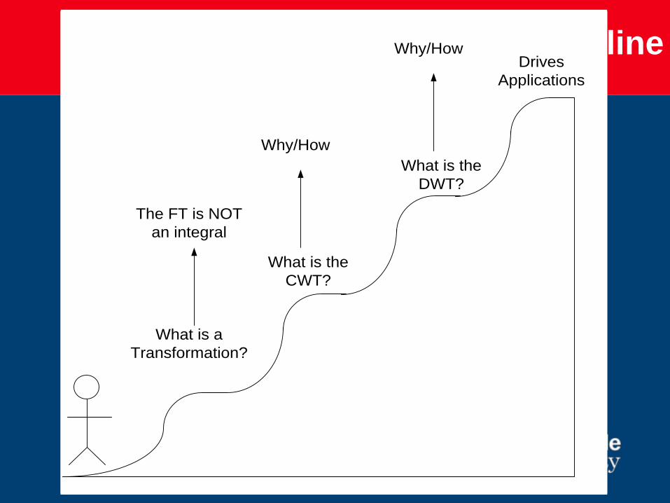
Outline
What is a
Transformation?
What is the
CWT?
What is the
DWT?
Drives
Applications
What is a
Transformation?
The FT is NOT
an integral
What is the
CWT?
What is the
DWT?
Drives
Applications
What is a
Transformation?
The FT is NOT
an integral
What is the
CWT?
Why/How
What is the
DWT?
Drives
Applications
What is a
Transformation?
The FT is NOT
an integral
What is the
CWT?
Why/How
What is the
DWT?
Why/HowDrives
Applications
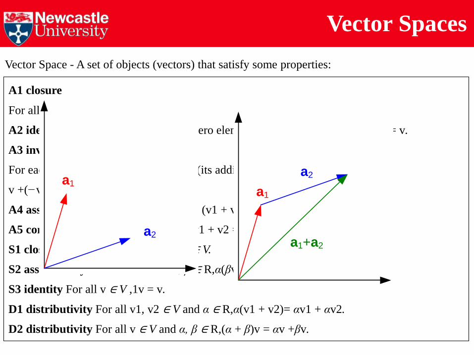
Vector Spaces
Vector Space - A set of objects (vectors) that satisfy some properties:
A1 closure
For all v1, v2 ∈ V , v1 + v2 ∈ V.
A2 identity For each v ∈ V , there is a zero element 0 ∈ satisfying v + 0 = 0 + v = v.
A3 inverses
For each v ∈ V , there is an element −v (its additive inverse) such that
v +(−v)= −v + v = 0.
A4 associativity For all v1, v2, v3 ∈ V , (v1 + v2)+ v3 = v1 +(v2 + v3).
A5 commutativity For all v1, v2 ∈ V ,v1 + v2 = v2 + v1.
S1 closure For all v ∈ V and α ∈ R,αv ∈ V.
S2 associativity For all v ∈ V and α, β ∈ R,α(βv)=(αβ)v.
S3 identity For all v ∈ V ,1v = v.
D1 distributivity For all v1, v2 ∈ V and α ∈ R,α(v1 + v2)= αv1 + αv2.
D2 distributivity For all v ∈ V and α, β ∈ R,(α + β)v = αv +βv.
a2
a1
a1+a2
a1
a2

Orthonormal vectors
Vector space S Basis:
A subset of vectors that can describe any other vector in S
21 bba 21 cc
Cartesian plane The x-y axes
22
1
ba
ba 1
c
c
?ic21111 bbbbab 21 ccOrthonormal
01 21 ccab1
Not Orthonormal
abb 11
221 ''
T
cc
b1
b2
a
b1
b2b'2
b'1
a
211 bbabbaa 2
Transformation
Inverse transformation
sinsin
coscos
22
1
aba
aba 1
c
c

A vector space = The set of all 2x2 matrices
A vector space = The set of all polynomials of order n or less
General VS
xixp2
31 2
22
5xxp
1 2
23 53 6
2 2p p
i x x p x
Inner product=
ax
ax
dxxpxpxpxppp 2*
12121, Length=
ax
ax
dxxpxp 11*
02
5
2
31
1
221
x
x
dxxxixpxp
12
3
2
31
1
11
x
x
dxxixixpxp lorthonorma, 21 xpxp
Rx
dxxpxpRL *2The set of all square integrable functions:
12
5
2
51
1
2222
x
x
dxxxxpxp
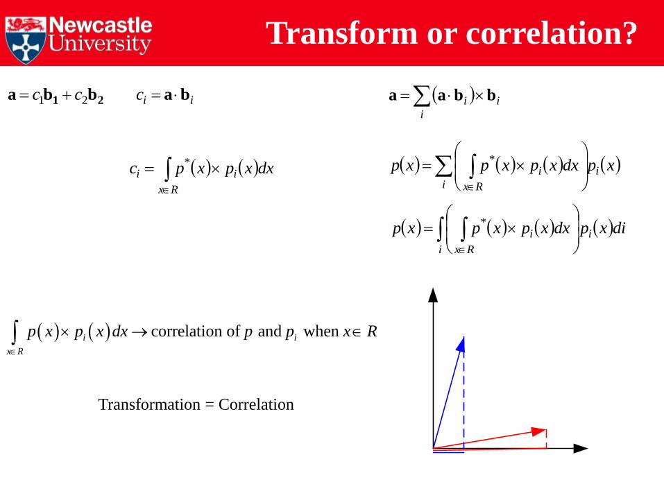
Transform or correlation?
21 bba 21 cc
xpdxxpxpxp i
i Rx
i
*
i
ii bbaa
correlation of and when i i
x R
p x p x dx p p x R
Transformation = Correlation
i
i
Rx
i dixpdxxpxpxp *
iic ba
Rx
ii dxxpxpc *
Correlation
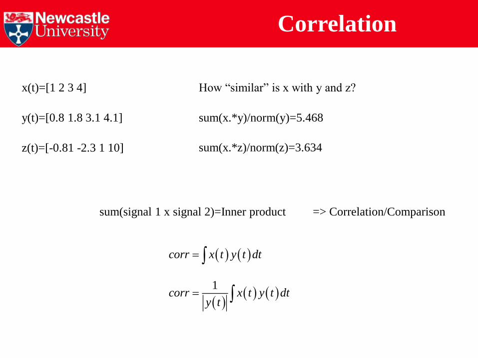
x(t)=[1 2 3 4]
y(t)=[0.8 1.8 3.1 4.1]
How “similar” is x with y and z?
z(t)=[-0.81 -2.3 1 10]
sum(x.*y)/norm(y)=5.468
sum(x.*z)/norm(z)=3.634
sum(signal 1 x signal 2)=Inner product => Correlation/Comparison
corr x t y t dt
1corr x t y t dt
y t

T(y)
yy1 y2 yn
T(y1)
T(yn)
T(y2)
Transformation
A detailed comparison (inner product) with a series of “test” signals
1 1 1c T y x t y t dt
x(t)
Any set of signals y can be used
For the inverse transformation, specific rules must be applied on the signals y (form a basis
in the vector space)
, {y1(t), y2(t),…}
T(y)
yy1 y2 yn
T(y1)
T(yn)
T(y2)
T(y)
yy1 y2 yn
T(y1)
T(yn)
T(y2)
T(y)
yy1 y2 yn
T(y1)
T(yn)
T(y2)
2 2 2c T y x t y t dt
n n nc T y x t y t dt
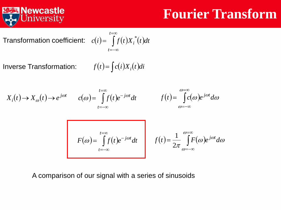
Fourier Transform
Transformation coefficient:
Inverse Transformation:
t
t
i dttXtfic*
ditXictf i
tji etXtX
t
t
tj dtetfc
dectf tj
t
t
tj dtetfF
deFtf tj
2
1
A comparison of our signal with a series of sinusoids

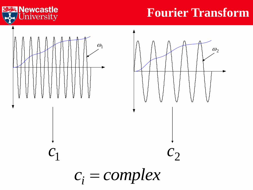
Fourier Transform
t
t
tj dtetfF
deFtf tj
2
1
A comparison of our signal with a series of sinusoids
sum(sin(0.5*t).*sin(t))=-5.281796023015190e-07sum(sin(2*t).*sin(0.5t))=2.112762663746470e-06sum(sin(0.5*t).*sin(0.5*t))=6.283185309820478e+02
t
Fourier Transform
1c 2c
complexci
12
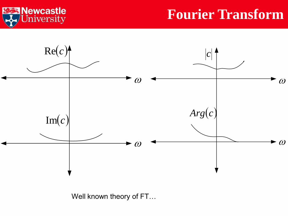
Fourier Transform
cRe
cIm
c
cArg
Well known theory of FT…

Fourier Transform as a Flow Chart
Choose Frequency ω
Compare x(t) with ejωT and get the
corresponding coefficient

Problems with the FT

Problems with the FT
t
Signal
t
Signal
Original signal
Rectangular
window
otherwise
atatrect
,0
,1,
atjtj dtetfdtetrecttfF
0
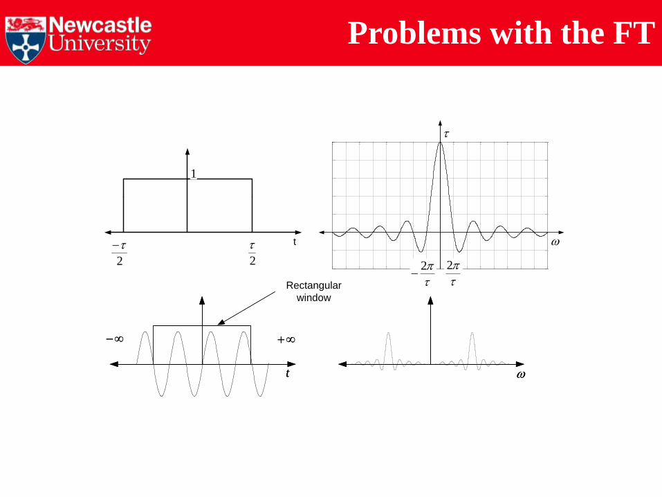
Problems with the FT
2
2
t
2
2
1
t
Rectangular
window
t

Problems with the FT
0 1 2 3 4 50
0.5
1
1.5
2
2.5
3x 10
7
frequency, Hz
2Hz @ 12.1Hz @ 0.5
0 1 2 3 4 50
0.5
1
1.5
2
2.5
3x 10
7
frequency, Hz
2Hz @ 12.1Hz @ 0.25
0 1 2 3 4 50
0.5
1
1.5
2
2.5
3x 10
7
frequency, Hz
2Hz @ 12.1Hz @ 0.1
To reduce the main lobe of the sinc() we must increase the length of the time window.

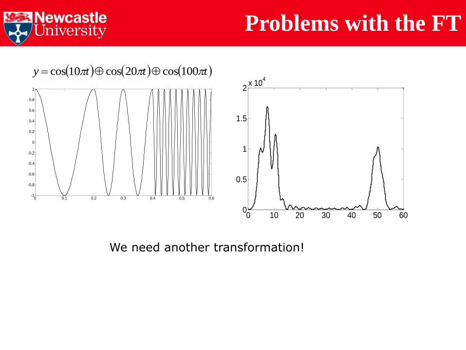
Problems with the FT
ttty 100sin20cos10cos
5 f, Hz
|F(f)|
10 50
0 0.1 0.2 0.3 0.4 0.5 0.6-3
-2
-1
0
1
2
3
0 10 20 30 40 50 600
2
4
6
8
10x 10
4
frequency, Hz
Problems with the FT
ttty 100cos20cos10cos
0 0.1 0.2 0.3 0.4 0.5 0.6-1
-0.8
-0.6
-0.4
-0.2
0
0.2
0.4
0.6
0.8
1
0 10 20 30 40 50 600
0.5
1
1.5
2x 10
4
We need another transformation!
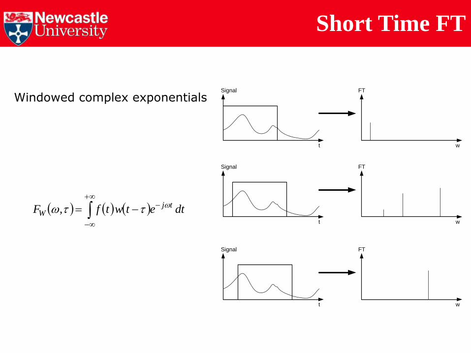
Windowed complex exponentials
t
Signal
w
FT
t
Signal
w
FT
t
Signal
w
FT
dtetwtfF tjW
,
Short Time FT
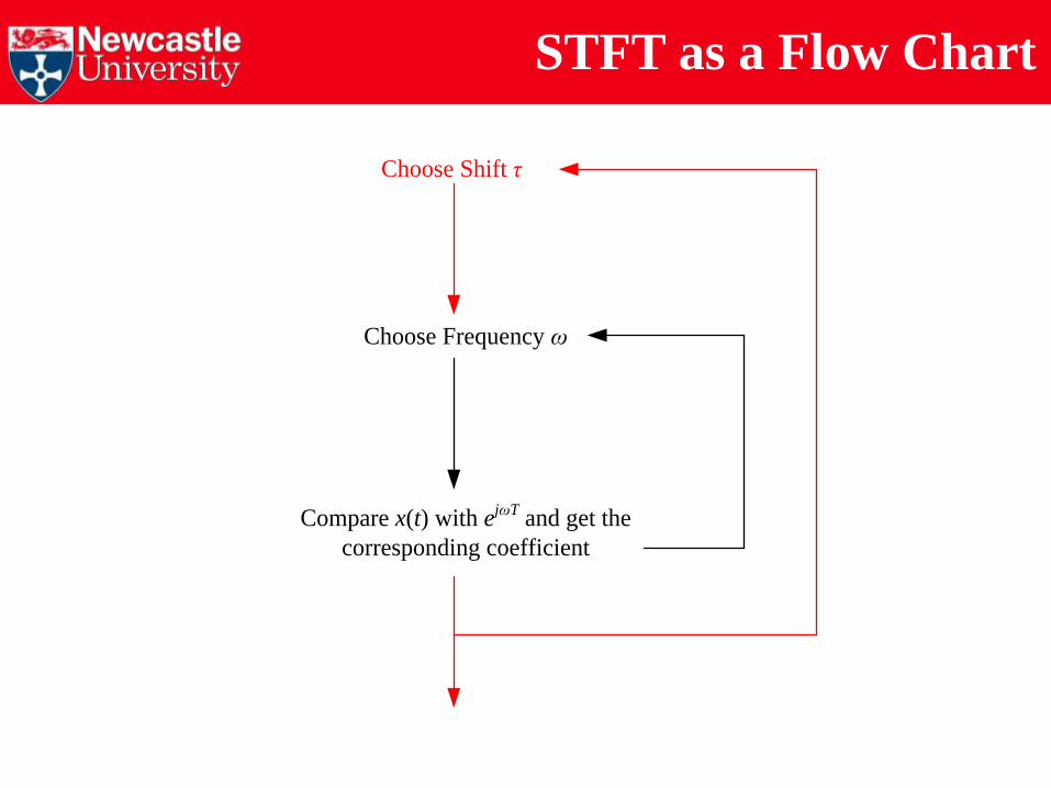
STFT as a Flow Chart
Choose Frequency ω
Compare x(t) with ejωT and get the
corresponding coefficient
Choose Shift τ

Capture each non stationary event in separate time windows
Time resolution
t
Time width
of window
Event 1 Event 2
t
Time width
of window
Event 1 Event 2

Frequency resolution
2
2
t
2
2
1
2
2
t
2
2
1

Frequency resolution
Capture each non stationary frequency in separate frequency windows
so that it will not be covered by the main lobe of the sinc function
f
Frequency width
of window
Event 1 Event 2
f
Frequncy 1
Frequency 2
Frequency width
of window

Frequency resolution
2
2
t
2
2
1
2
2
t
2
2
1
Decreasing time window=>Increase frequency window
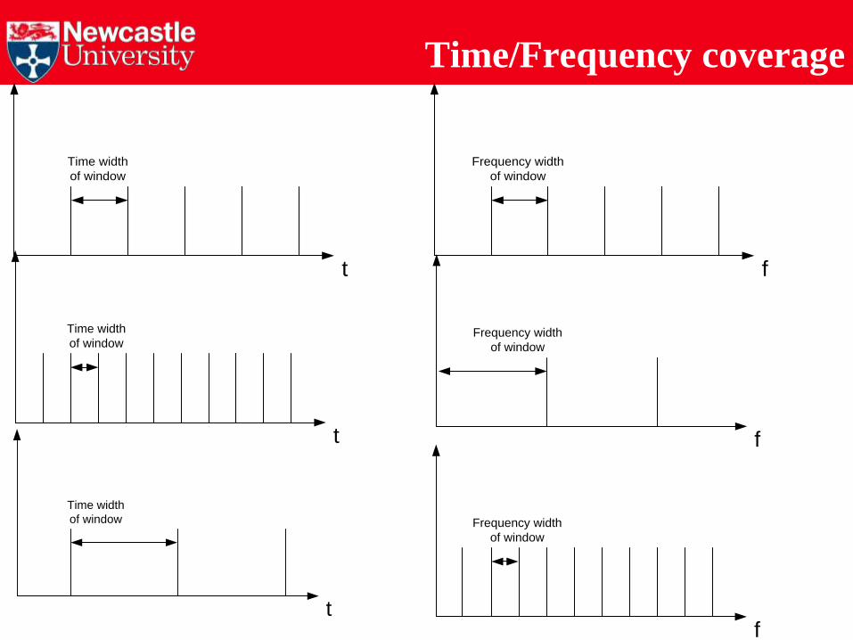
Time/Frequency coverage
t
Time width
of window
f
Frequency width
of window
t
Time width
of window
f
Frequency width
of window
t
Time width
of window
f
Frequency width
of window

Time/Frequency Plane
t
t
f
f
4
1 ft
Heisenberg uncertainty theory
t
t
f
f
t
t
f
f
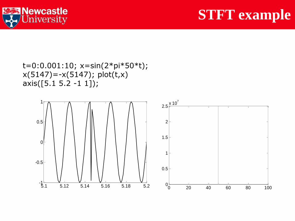
t=0:0.001:10; x=sin(2*pi*50*t);x(5147)=-x(5147); plot(t,x)axis([5.1 5.2 -1 1]);
5.1 5.12 5.14 5.16 5.18 5.2-1
-0.5
0
0.5
1
0 20 40 60 80 1000
0.5
1
1.5
2
2.5x 10
7
STFT example
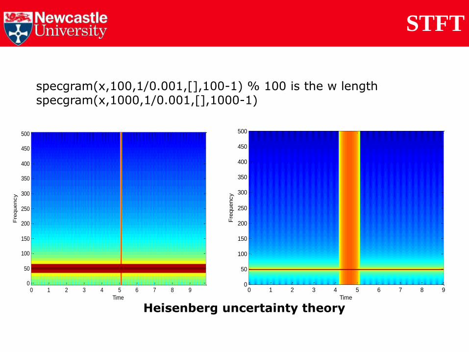
specgram(x,100,1/0.001,[],100-1) % 100 is the w lengthspecgram(x,1000,1/0.001,[],1000-1)
Time
Fre
quency
0 1 2 3 4 5 6 7 8 90
50
100
150
200
250
300
350
400
450
500
Time
Fre
quency
0 1 2 3 4 5 6 7 8 90
50
100
150
200
250
300
350
400
450
500
Heisenberg uncertainty theory
STFT

Wavelet transformation
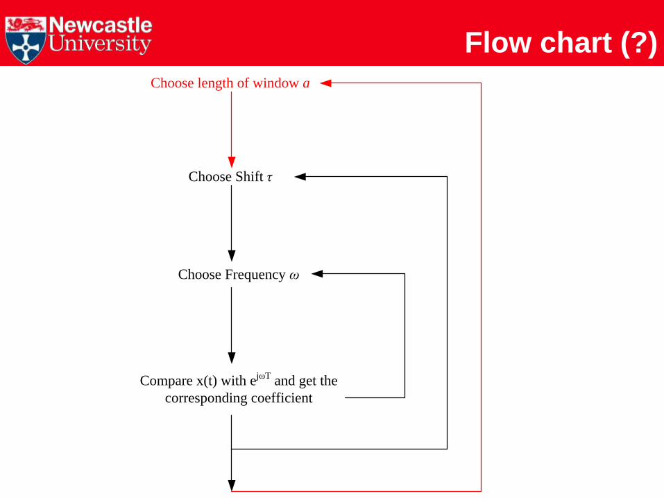
Flow chart (?)
Choose Frequency ω
Compare x(t) with ejωT and get the
corresponding coefficient
Choose Shift τ
Choose length of window a

Varying windows
t
Mother wavelet
“3D Transformation”: frequencies, scales, shifts and coefficients
Combine scales with frequencies => 2D Transformation
Low frequency components => long duration High frequency components => short duration

Wavelet - Correlation
a
b
c
a
bt
atba
1)(,
dt
a
bttx
abaT *)(
1,

Wavelet Transform – Time Domain
2/2 2
1 tett 2/2
2
11
a
bt
ea
bt
aa
bt
-8 -6 -4 -2 0 2 4 6 8-1
-0.5
0
0.5
1
1.5
a=1
a=2
a=0.5
5.0a
1a
2a
2/22
11
a
t
ea
t
aa
t

Wavelet Transform – Frequency Domain
0 0.2 0.4 0.6 0.8 10
1
2
3
4
5
6
7x 10
4
a=1
a=2
a=0.5
2a
1a
5.0a
-8 -6 -4 -2 0 2 4 6 8-1
-0.5
0
0.5
1
1.5
a=1
a=2
a=0.5
5.0a
1a
2a
Wavelet => bandpass filter
Low frequency components => long duration High frequency components => short duration
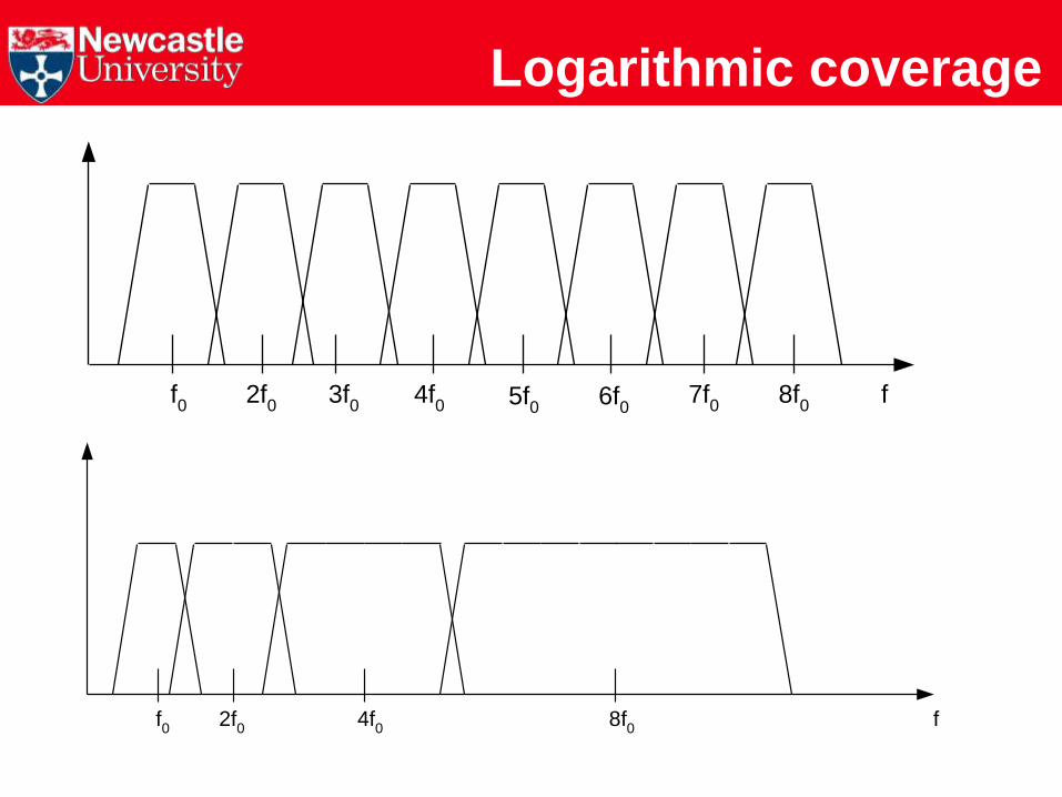
Logarithmic coverage
f0
2f0
4f0
8f0
f
f0
2f0
4f0
8f0
f3f0 5f
06f
07f
0
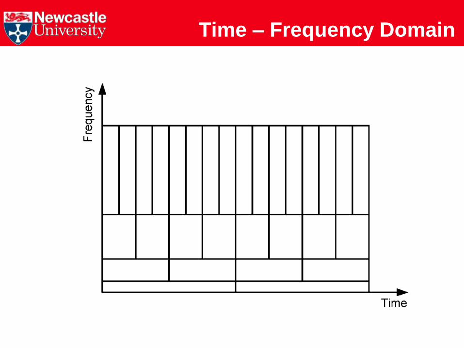
Time – Frequency Domain
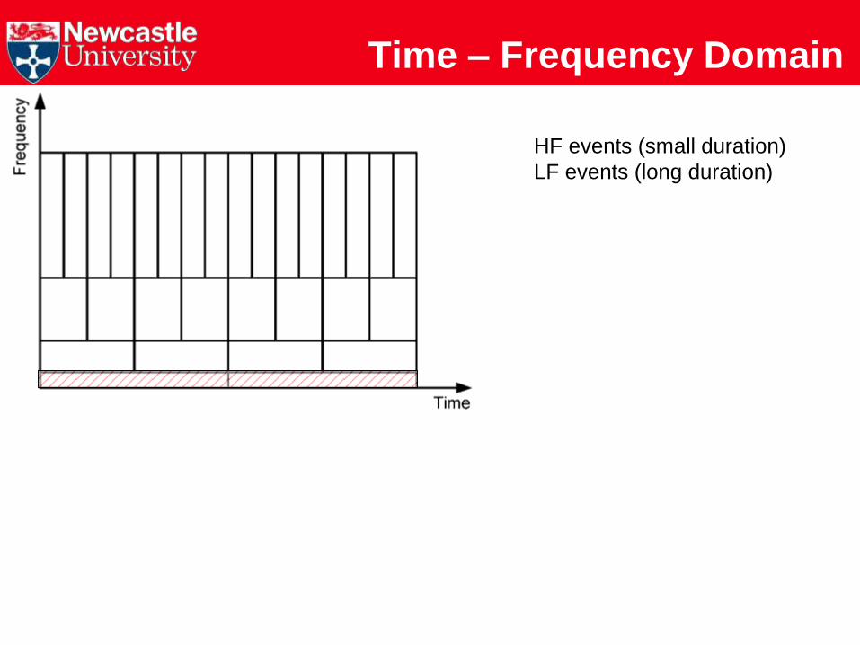
Time – Frequency Domain
HF events (small duration)
LF events (long duration)

Wavelet Transform - Reconstruction
0
2,,1)(
a
dbdaTCtx baba
dC12
2
Admissibility constant
0)( dtt Wave…
dtt)(2 …let
Wavelet
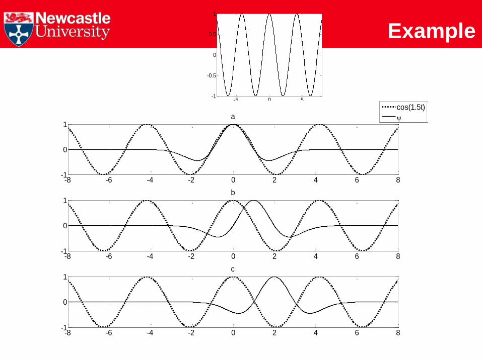
Example
-5 0 5-1
-0.5
0
0.5
1
-8 -6 -4 -2 0 2 4 6 8-1
0
1a
-8 -6 -4 -2 0 2 4 6 8-1
0
1b
-8 -6 -4 -2 0 2 4 6 8-1
0
1c
cos(1.5t)

Example cont…
-5 0 5-1
0
1
-5 0 5-1
0
1
-5 0 5-1
0
1

c=cwt(x,scales, wavelet,plot);
Example cont…
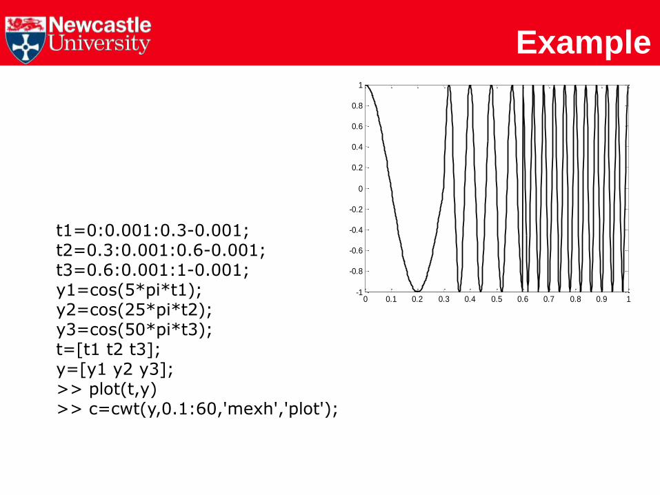
Example
0 0.1 0.2 0.3 0.4 0.5 0.6 0.7 0.8 0.9 1-1
-0.8
-0.6
-0.4
-0.2
0
0.2
0.4
0.6
0.8
1
t1=0:0.001:0.3-0.001;t2=0.3:0.001:0.6-0.001;t3=0.6:0.001:1-0.001;y1=cos(5*pi*t1);y2=cos(25*pi*t2);y3=cos(50*pi*t3);t=[t1 t2 t3];y=[y1 y2 y3];>> plot(t,y)>> c=cwt(y,0.1:60,'mexh','plot');
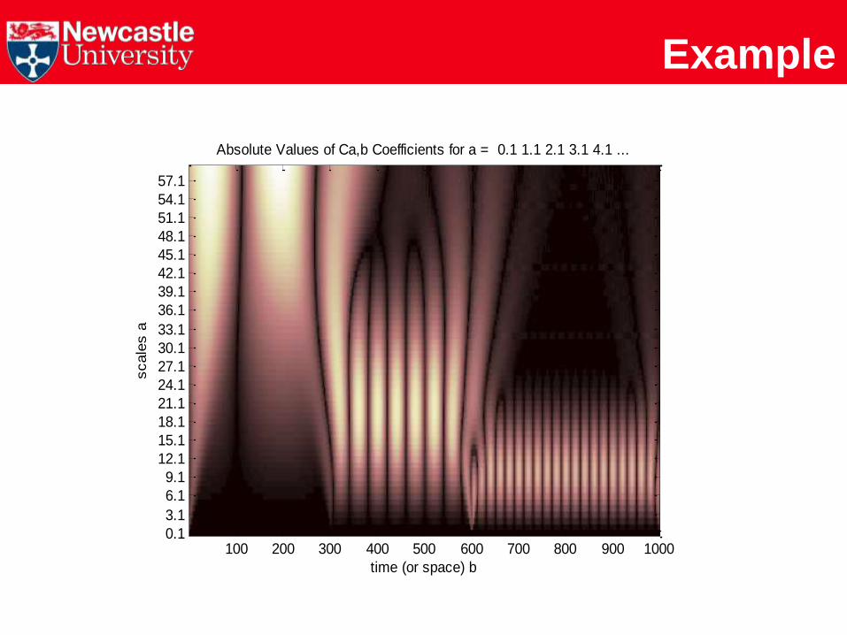
Example
Absolute Values of Ca,b Coefficients for a = 0.1 1.1 2.1 3.1 4.1 ...
time (or space) b
scale
s a
100 200 300 400 500 600 700 800 900 1000 0.1
3.1
6.1
9.1
12.1
15.1
18.1
21.1
24.1
27.1
30.1
33.1
36.1
39.1
42.1
45.1
48.1
51.1
54.1
57.1

Example
t=0:0.001:10; x=sin(2*pi*50*t);x(5147)=-x(5147); plot(t,x)axis([5.1 5.2 -1 1]);
5.1 5.12 5.14 5.16 5.18 5.2-1
-0.5
0
0.5
1
>>c=cwt(x,1:50,'mexh','plot');
Absolute Values of Ca,b Coefficients for a = 1 2 3 4 5 ...
time (or space) b
scale
s a
1000 2000 3000 4000 5000 6000 7000 8000 9000 10000
1
2
3
4
5
6
7
8
9
10
11
12
13
14
15
16
17
18
19
20

Edge Detection
+
- +
- +
+
- -t
t
t
-+
- +t
-
+ +t
-
WT coefficient=0
WT coefficient=“Max”
Increase
Suddenly
WT coefficient=0
WT coefficient=“Min”
Decrease
WT coefficient=0
Increase
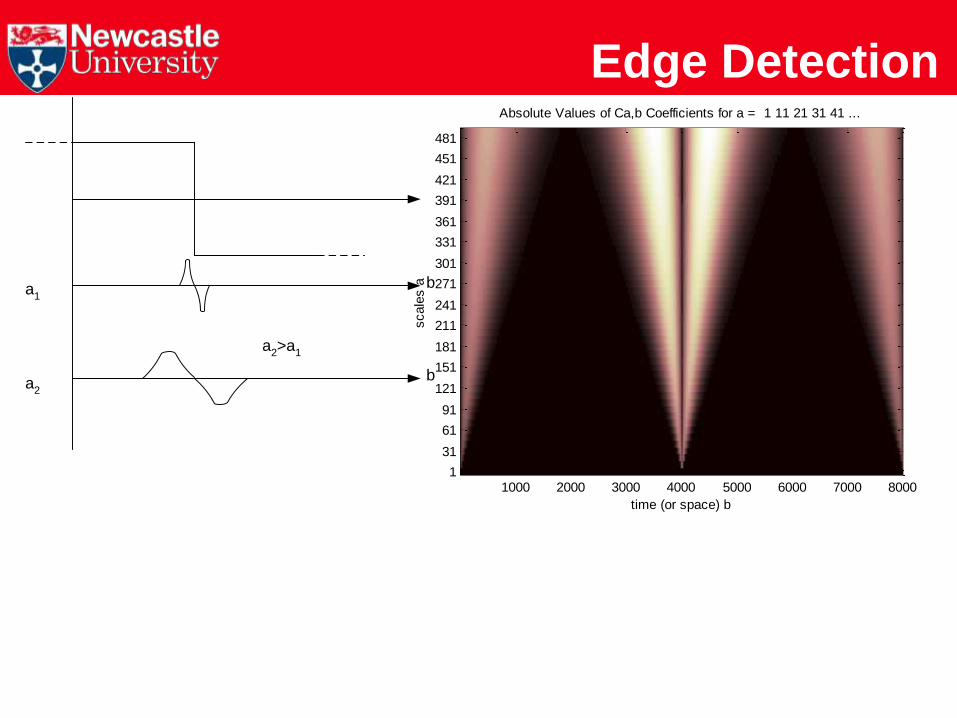
Edge Detection
b
b
a1
a2
a2>a
1
Absolute Values of Ca,b Coefficients for a = 1 11 21 31 41 ...
time (or space) b
scale
s a
1000 2000 3000 4000 5000 6000 7000 8000 1
31
61
91
121
151
181
211
241
271
301
331
361
391
421
451
481

Fast Wavelet Transformation

Discrete WT: Frames
baba xdttxbaT ,*, ,)(),(
Orthonormal transformation?
We have to use every possible scale from 0 to
and every possible shift from to
“Two times infinite fundamental components”
Can we choose only a set of scales and shifts
so that we will have a true orthonormal transformation?
Yes but we need more restrictions, i.e. “better wavelets”
mm anbbaa 000 ,
m
m
mnmbaa
anbt
att
0
00
0
,,
1)()(
nmm
m
mxdt
a
anbt
atxnmT ,
0
00
0
,*1
)(),(
Tm,n are called wavelet
or detail coefficients
Discrete WT: Frames
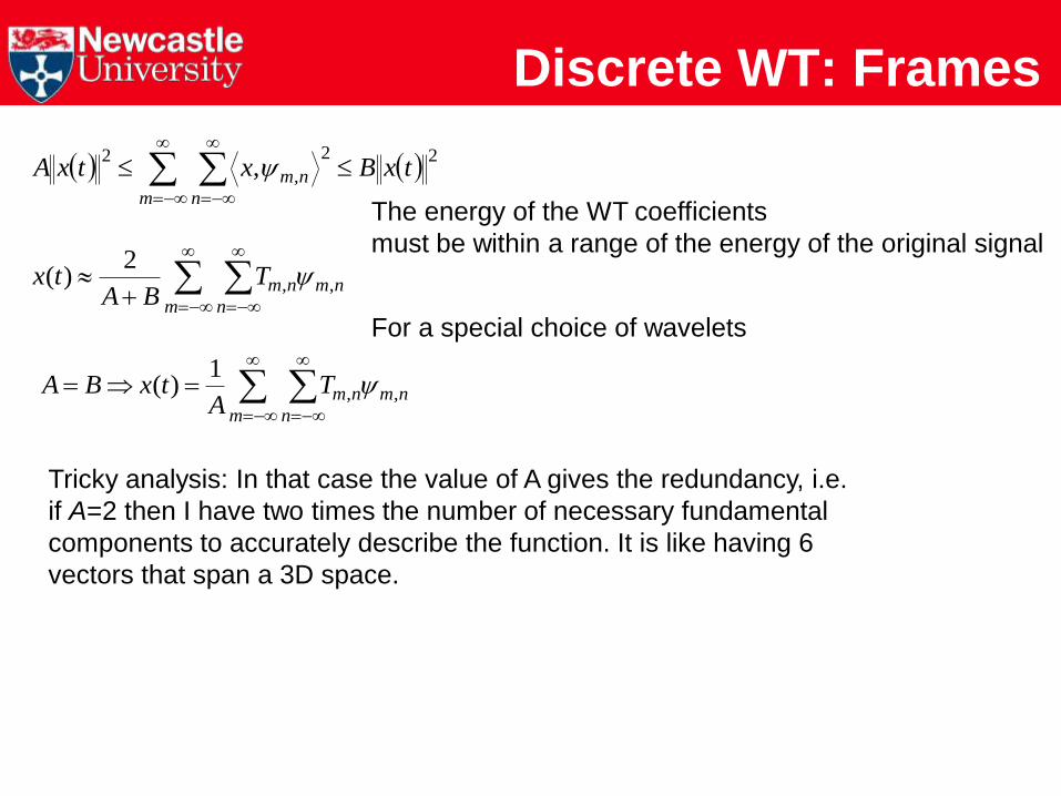
22
,
2, txBxtxA
m n
nm
m n
nmnmTBA
tx ,,
2)(
m n
nmnmTA
txBA ,,
1)(
Tricky analysis: In that case the value of A gives the redundancy, i.e.
if A=2 then I have two times the number of necessary fundamental
components to accurately describe the function. It is like having 6
vectors that span a 3D space.
The energy of the WT coefficients
must be within a range of the energy of the original signal
For a special choice of wavelets
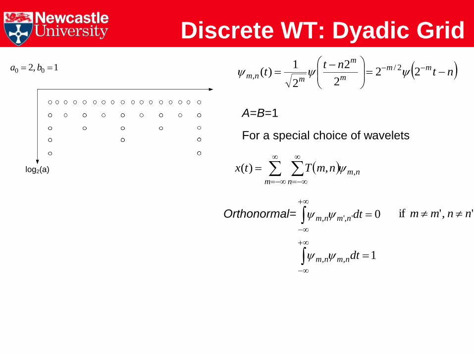
Discrete WT: Dyadic Grid
1,2 00 ba
log2(a)
ntnt
t mm
m
m
mnm
22
2
2
2
1)( 2/
,
A=B=1
m n
nmnmTtx ,,)(
0',',
dtnmnm Orthonormal= ',' if nnmm
1,,
dtnmnm
For a special choice of wavelets
Special Wavelets???
No big problem as Matlab has many wavelets that can be used to DWT
Daubechies (DB) wavelets
Our problems just began!
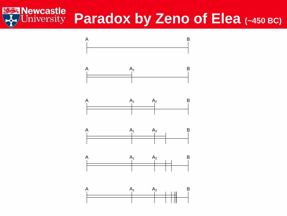
Paradox by Zeno of Elea (~450 BC)
A B
A BA1
A BA1 A2
A BA1 A2
A BA1 A2
A BA1 A2

Scaling Function
2
0B
2
0f
1m
t12
0B
0f
0m
t02
4
0B
4
0f
2m
t22
m m
0B
0f
20B
20f
40B
40f
0m1m
20 mm
t02 t12 t22
m m
t22
0
0 ,,)()(m
m n
nmm nmTtxtx
Note: WT coefficients = Output of a BP filter
Note: SF coefficients = Output of a LP filter

DWT: Multiresolution
30m 2
0m 1
0m
0mm
0md10md20md30md
0mS
10md20md30md
20 mS 20 mT
20md30md
10 mS 10 mT
)(0 nxS
LP 2
2
2
2
nT ,1
nS ,1
nT ,2
nS ,2
HP
LP
HP
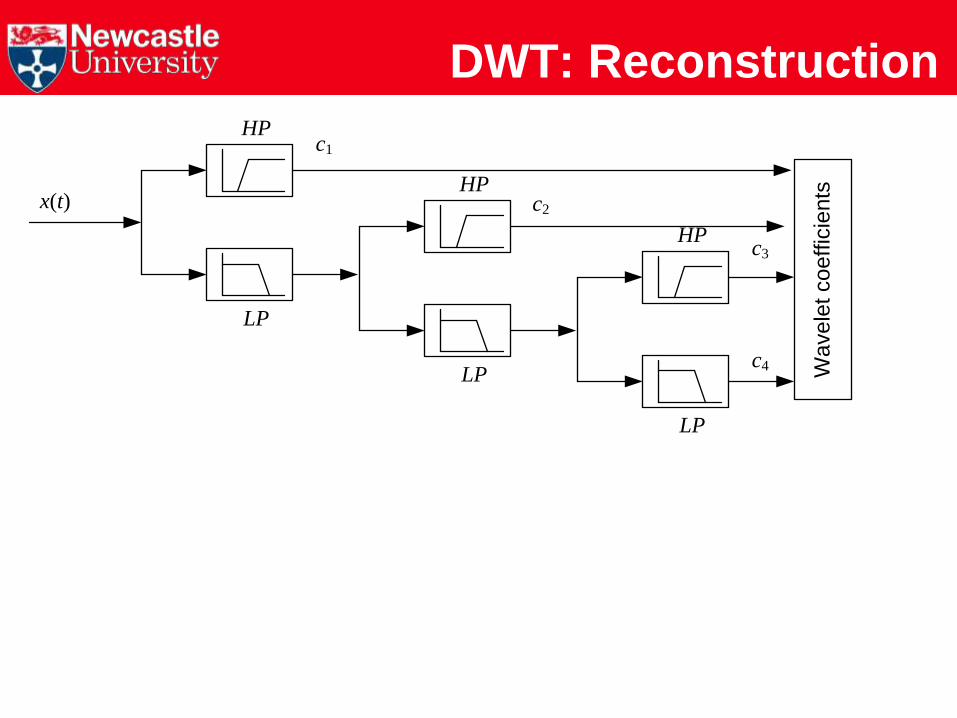
DWT: Reconstruction
x(t)
HP
LP
HP
LP
HP
LP
c1
c2
c3
c4 Wa
ve
let co
effic
ien
ts

DWT: Reconstruction
0mS
knkmkSc 2,0
knkmkSb 2,0
10mS
knkmkSc 2,10
knkmkSb 2,10
10mT
20mS
20mT
kkmkn Sc ,2 0
kkmkn Sb ,2 0
knkmkSb 2,0
+
+ +
+
0mS
More levels (more scales) => Better analysis
But we add delays!!!
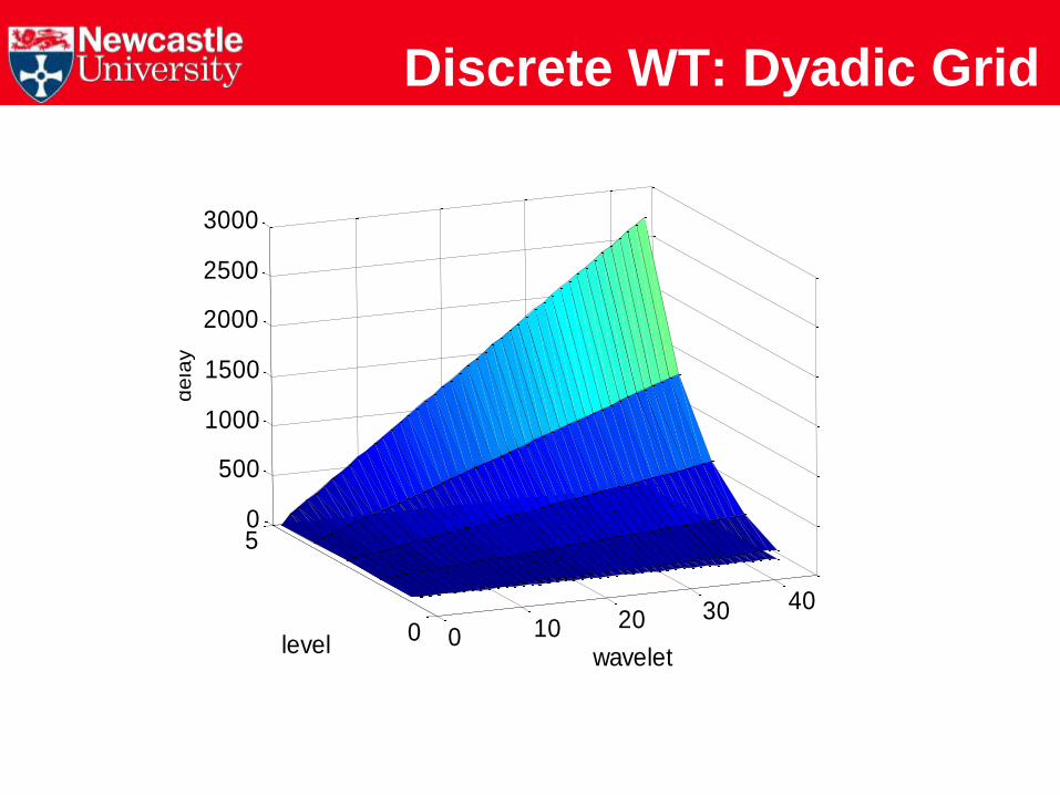
Discrete WT: Dyadic Grid
0 10 20 30 40
0
50
500
1000
1500
2000
2500
3000
waveletlevel
de
lay

Applications

Applications
SignalDWT
Wavelet coefficientsProcess
Useful
information
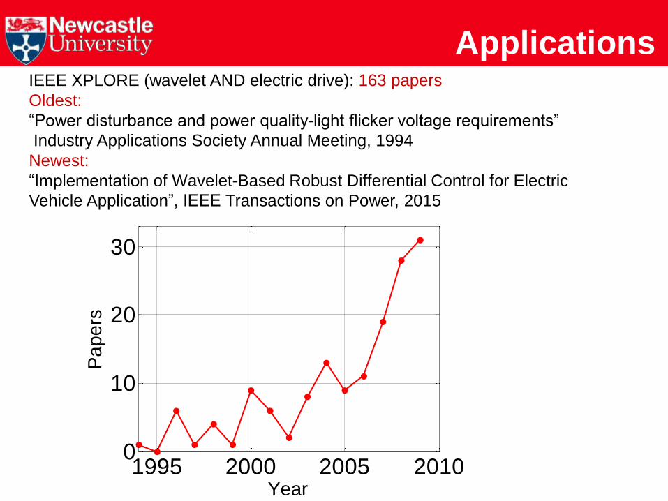
ApplicationsIEEE XPLORE (wavelet AND electric drive): 163 papers
Oldest:
“Power disturbance and power quality-light flicker voltage requirements”
Industry Applications Society Annual Meeting, 1994
Newest:
“Implementation of Wavelet-Based Robust Differential Control for Electric
Vehicle Application”, IEEE Transactions on Power, 2015
1995 2000 2005 20100
10
20
30
Year
Papers

Controller DesignIEEE IA, Khan et al, 2008“Implementation of a New Wavelet Controller for Interior Permanent-Magnet Motor Drives”
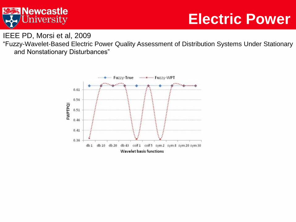
Electric PowerIEEE PD, Morsi et al, 2009“Fuzzy-Wavelet-Based Electric Power Quality Assessment of Distribution Systems Under Stationary
and Nonstationary Disturbances”
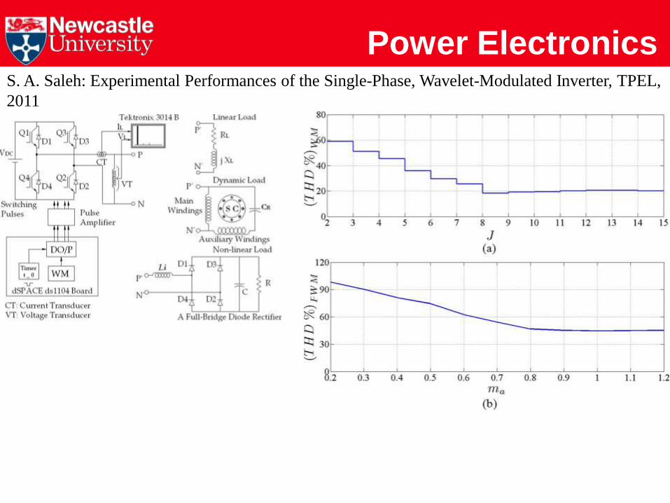
Power ElectronicsS. A. Saleh: Experimental Performances of the Single-Phase, Wavelet-Modulated Inverter, TPEL,
2011
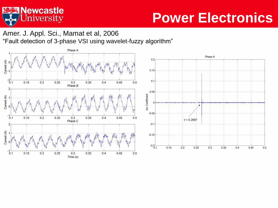
Power ElectronicsAmer. J. Appl. Sci., Mamat et al, 2006“Fault detection of 3-phase VSI using wavelet-fuzzy algorithm”

Fault DetectionIEEE IA, Douglas et al, 2004
“A New Algorithm for Transient Motor Current Signature Analysis Using Wavelets”

Denoising
NoiseNoiseNoise
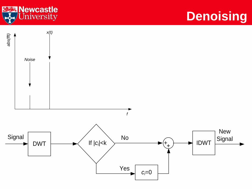
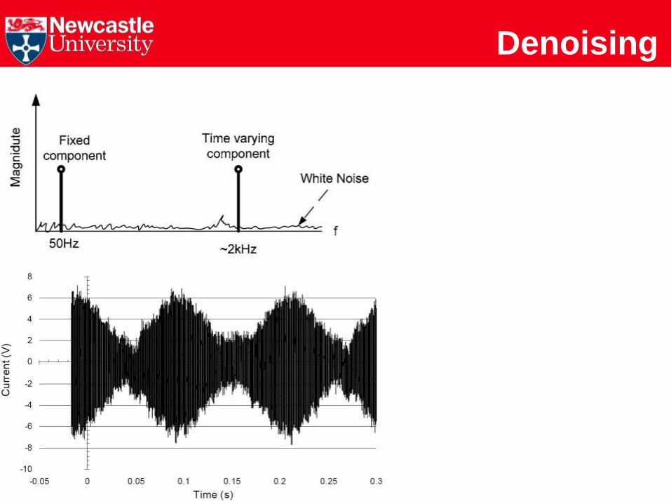
Denoising
SignalDWT IDWT
New
SignalIf |ci|<k
No
Yesci=0
++
Noise
x(t)
f
ab
s(f
ft)

DenoisingIEEE IE Giaouris at el, 2008,
“Wavelet denoising for electric drives”
Denoising

Denoising

DWT and KF

DWT and KF

DWT and KF
i. r=0.1 and the KF has the correct information directly
ii. r=0.1 and the KF has the correct information from the WT
iii. r=0.1 and the KF assumes r=0.01

Any questions?

Millennium Bridge – Newcastle upon Tyne