a set of descriptors for automatic classification of

264

A SET OF DESCRIPTORS FOR AUTOMATIC CLASSIFICATIONOF SCATTERERS IN SEISMIC SECTIONS

S. Maciel and R. Biloti

email: [email protected]: Machine Learning, SVM, diffractions, descriptors

ABSTRACT

Seismic diffractions are mainly induced by edges, tips and small structures, so diffraction imaging canextract valuable information to identify subsurface scattering features. We investigate the possibilityto image and characterize diffractions using pattern recognition methods. To this end, we look atkinematical and dynamical aspects of diffraction operators under a determined velocity model andwe propose a set of attributes that better distinguish diffractions from reflections. These attributes areused as descriptors of imaging points on a seismic section to perform automatic classification usingsupervised and unsupervised algorithms. We evaluate the method using synthetic and GPR data.For synthetic data, we show results from amplitudes picking within a range of error on velocities toindicate the method sensivitness on velocity model. For real datasets, velocity analysis is performed.Results indicate that the method is robust even for low signal-to-noise ratio datasets.

INTRODUCTION

The theory of seismic wave propagation in acoustic media is used to unriddle seismograms into realisticEarth models. Traditional processing of seismic data generally uses information from the reflected wave-field to obtain images of interfaces at the subsurface. An important aspect when interpreting subsurface im-ages is the identification of small scale features, such as faults, channels and fractures. Instead of promotingreflections, seismic energy interacting with these structures results in diffractions, when their dimensionsare smaller than the acoustic wavelength emitted during seismic acquisition (Trorey, 1970; Klem-Musatov,1994). This information has been used for high-resolution imaging (Khaidukov et al., 2004; Fomel et al.,2007) or local velocity analysis (Sava et al., 2005; Reshef and Landa, 2009).

Even though theoretical studies on diffracted waves have been developed in detail since 1962, with theremarkable work of Keller (1962) on the geometrical theory of diffractions, diffraction imaging is beingconsidered by oil and gas industry only for a few years until today, mainly within regions with high densityof fractures, such as shales and carbonates. Recent works on this theme can be found on Sturzu et al.(2014); Kowalski et al. (2014); Burnett et al. (2015); Grasmueck et al. (2015)

Diffracted seismic waves are characterised by some peculiar attributes. Trorey (1970) showed analit-ically that for a single truncated plane reflector, the phase of the diffractions suffers a reversal of 180◦

on either side of the reflecting edge. Diffracted waves are recorded as significantly lower energy than re-flected waves. Their amplitudes decay faster than it would be by simple geometrical spreading, what makesdiffractions to be treated as noise in traditional seismic processing. These phenomena can also be observedon seismograms of controlled experiments of physical modeling of a simulated fault (Hilterman, 1970).

In isotropic media, diffraction traveltimes are approximated by a conventional double-square-root(DSR) equation. The amplitudes extracted along the elementary diffractions, known as the diffractionoperator, forms a curve that was used by Tabti et al. (2004) to determine the so-called Fresnel aperture,used to enhance Kirchhoff-type depth-migration.

Annual WIT report 2015 265

0

1

2

3

4

t (

s)

500 1000 1500 2000 2500 3000 3500 4000 4500Horizontal coordinate (m)

(a) Synthetic dataset. (b) Fresnel aperture.

Figure 1: Left: Synthetic dataset. Right: Top - Diffraction operator associated with a reflection (a) and avoid point (b). Vertical axis is the amplitude, and horizontal axis is the horizontal coordinate of mid point.Middle - Diffraction traveltime is tangent to the reflection traveltime at the specular reflection event (a).For void points , there is no tangency to any events, and the diffraction operator shows random peaks (b).Bottom - Location in depth of the imaging point associated with a reflection (a) and a void point (b).

Tabti et al. (2004) proposed a version of Kirchhoff migration with Fresnel aperture selection, whichprovides better resolution on reflection imaging. Diffraction imaging may be performed if part of theamplitude inside reflection Fresnel aperture is removed (Bona and Pevzner, 2015). According to Tabti et al.(2004), to every image point y it is associated a diffraction operator d(y), which is a vector of dimension n,the number of traces in the section. Each element of d(y) is defined as dk = W (ξk, y)∂tU(ξk, t)|t=τD(ξk,y)

and ξk is the coordinate that parametrizes the k-th trace, is defined as the vector of all seismic amplitudesto be stacked by a Kirchhoff migration for imaging point y and midpoint coordinate ξ. W (ξ, y) is a weightfunction, U(ξ, t) is the seismic data measured at position ξ and time t, and τD(ξ, y) is the traveltime ofthe elementary diffraction of a point scatterer in y. In isotropic media with small lateral variations on thevelocity model, for a common-offset configuration τD is computed by double-square root approximation

τD(ξ; y) =

√(t02

)2

+

(ξ − h− ξyvrms

)2

+

√(t02

)2

+

(ξ + h− ξyvrms

)2

, (1)

where t0 is the zero-offset two-way time for image point y, ξy is the coordinate of y, h is the half-offsetand vrms is the RMS velocity. In this study, for diffration imaging in time we use the Double SquareRoot equation in the limits of time migration. For diffraction imaging in depth, we use paraxial traveltimecalculation provided by Seismic Unix package (Cohen and Stockwell, 2013).

Attributing to point y the sum of elements of d(y) over the migration aperture leads to Kirchhoff mi-gration.

A diffraction traveltime curve associated to an image point located on a reflector is tangent to thereflection traveltime at the specular reflection event (see Fig. 1(b))(Schleicher et al., 1997). This pointbecomes a tangential region when the source has limited bandwidth, which is defined by Tabti et al. (2004)as Fresnel aperture, and by Schleicher et al. (1997) as the minimum aperture for true-amplitude depthmigration. As illustrated on Fig. 2(a), the Fresnel aperture turns the diffraction operator associated with areflector to have a plateau shape. In the case of a tip or edge scatterer, the associated elementary diffractiontraveltime corresponds to the diffracted seismic event. Thus, its Fresnel aperture extends theoretically toinfinity, and the diffraction operator shape will vary according to the nature of the scatterer: with a 180◦

phase shift if an edge diffraction, or an approximated gaussian shape if a point scatterer (see Fig. 2(a)).This fact is used by Figueiredo et al. (2013) to classify imaging points. They apply a two-class k nearest

neighbours (kNN) pattern recognition technique to amplitudes along diffraction operators to distinguishbetween diffractions, reflections or absence of scattering energy.

266 Annual WIT report 2015

(a) Amplitudes. (b) Histograms.

Figure 2: Left: Amplitudes collected along indicated curves on Figure 1(a). Point scatterer diffraction op-erator (top); Edge diffraction operator (middle); Diffraction operator associated with a reflection (bottom).Right: Diffraction operators’ associated PDFs are similar to their histograms.

We present a set of routines to perform automatic detection of diffractions on unmigrated data usingpattern recognition techniques. We propose an extension of Figueiredo et al. (2013) approach to diffractionimaging, using a set of features to better distinguish diffraction operators. Classification is performed withMachine Learning algorithms. For the diffraction imaging task, we have used Support Vector Machines(SVM), after a study by Kotsiantis et al. (2006) pointing that SVM approach can present the best accuracyfor classification of a waveform dataset. The next session includes a brief Machine Learning background,explaining how SVM works.

MACHINE LEARNING BACKGROUND

Machine learning is an intersection field between computer science and statistics, that explores the con-struction of algorithms that can learn from and make predictions on data. Such algorithms operate bybuilding a model from a set of input examples in order to accomplish a given task, rather than followingstrictly static program instructions to make data-driven predictions.

Input examples are numerically described by an ensemble of quantities that characterizes an object,denominated descriptor. The object may not be entirely described by the descriptor, but descriptors fordifferent classes of objects should be different enough to allow the discrimination of the objects.

A descriptor is composed by experimental measures, or theoretical calculations that describe the struc-ture of the object. The major hypothesis is that descriptors capture some important characteristic of theobject, and then a mathematical function can generate a mapping between the descriptor space and a prop-erty space, where classes are defined. Another hypothesis is that objects with similar descriptors must havesimilar properties. In many cases, the task of building descriptors is equivalent to find the best classifier fora problem.

Learning algorithms are employed for classification or regression tasks. In classification, inputs aredivided into two or more classes, and the algorithm must produce a model that assigns unseen inputs toone or more of these classes. The algorithms usually has two main phases: training and testing. On the


training stage, a training set of objects is used by the learner to build a general model about the space giventhat enables it to make predictions in new samples. The training set usually comes from some unknownprobability distribution, but must be considered representative of the space of occurrences. Learning can besupervised or unsupervised. Pattern recognition methods that exploit a priori known information about thetraining data set are known as supervised pattern recognition, or in the more general context of machinelearning, as supervised learning.

For instance, consider a seismic common-offset gather as input dataset for learning. The set of imagingpoints of the section, denoted here by Y , is the set of objects to be classified. A descriptor γ : Y → Fmaps an object y ∈ Y onto a feature f ∈ F on the feature space F . The elements in F are then mappedonto an instance space L = {ω1, . . . , ωl}, by the classifier θ : F → L. The set of classes L might be,for example, composed by the classes point diffraction (ω1), edge diffraction (ω2), reflection (ω3) or voidpoint (ω4). With a good representation of the input space in the training phase, further imaging points areautomatically classified by the algorithm.

There are some well known Machine Learning techniques for clustering and classification of data.Further references are found for example on Theodoridis and Koutroumbas (2009).

METHOD

Building a descriptor for classification

Let the seismic section be represented by Y , a common-offset gather in our case. The objects to be classi-fied are imaging points y ∈ Y . Figueiredo et al. (2013) used the diffraction operators presented by Tabtiet al. (2004) as descriptor. In other words, Figueiredo et al. set their descriptor as d(y) and the featurespace as Rn (recall that n is the number of traces in the input common-offset section). This implies that thedimension of the feature space is dependent on the geometry of the common-offset gather, which is datasetdependent. Classification is performed by kNN algoritm, where training data is composed by diffractionoperators associated with scatterer imaging points, labeled as diffractions, and diffraction operators associ-ated with void image points, labeled as noise. In other words, their classifier θF maps vectors of Rn to ω1

(meaning diffraction) or ω2 (meaning noise). The training dataset Tf ⊂ Rn is built manually by the user,from a synthetic dataset with the same geometry of the common-offset to be analyzed, where the exactposition and nature of the scatterers are known. They used Euclidean distance to measure the distancebetween neighbours.

We propose different choices for the feature space and descriptor. Instead of using the diffraction op-erator itself as the descriptor, we compute some quantities from the diffraction operator, which are lessdependent of the geometry of the dataset. In other words, our descriptor γ is defined as γ(y) = φ(d(y)),where φ is a set of measures of d(y). Thus, our feature space is Rm, where m is the number of character-istics quantities computed from d(y). Usually, m � n. This has the side effect to make the classificationproblem cheaper when compared to the strategy of Figueiredo et al. (2013).

What makes diffractions different from reflections on the diffraction operator space Rn is essentiallytheir shapes. For each imaging point, the associated diffraction operator is seen as a random variable. Inthis way, φ(d(y)) is a set of shape parameters of the probability distributions associated to the amplitudesof diffraction operators. Figure 2(b) shows the histograms of diffraction operators associated with an edgediffraction, a point diffraction and a reflection. The histogram is a tool to show the frequency function ofa distribution, or the number of sample values falling into a certain specified range. To build a histogram,one must take every class interval as the basis of a rectangle with height v

ph , where v denotes the numberof sample values in the class, h is the length of the class interval and p is the number of classes. The areaof any rectangle in the histogram is equal to the corresponding class frequency v

p . For large p this may beexpected to be approximately equal to the probability that an observed value of the variable will belong tothe corresponding class interval, which is equal to the integral of the frequency function over the interval.This means that the histograms of diffraction operators are similar to their respectives Probability DensityFunctions, if diffraction operators are seen as random variables. (For references on histograms see, forexample, Cramer (1946)).

Statistical measures, such as skewness and kurtosis are commonly as used shape parameters of probabil-ity densities (Theodoridis and Koutroumbas, 2009). In Statistics, skewness is a measure of the asymmetry


(a) Sum (b) Standard Deviation

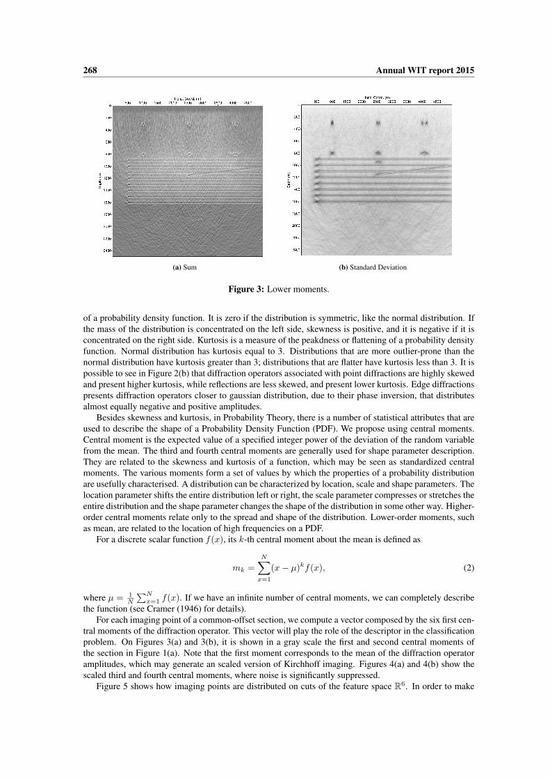
Figure 3: Lower moments.

of a probability density function. It is zero if the distribution is symmetric, like the normal distribution. Ifthe mass of the distribution is concentrated on the left side, skewness is positive, and it is negative if it isconcentrated on the right side. Kurtosis is a measure of the peakdness or flattening of a probability densityfunction. Normal distribution has kurtosis equal to 3. Distributions that are more outlier-prone than thenormal distribution have kurtosis greater than 3; distributions that are flatter have kurtosis less than 3. It ispossible to see in Figure 2(b) that diffraction operators associated with point diffractions are highly skewedand present higher kurtosis, while reflections are less skewed, and present lower kurtosis. Edge diffractionspresents diffraction operators closer to gaussian distribution, due to their phase inversion, that distributesalmost equally negative and positive amplitudes.

Besides skewness and kurtosis, in Probability Theory, there is a number of statistical attributes that areused to describe the shape of a Probability Density Function (PDF). We propose using central moments.Central moment is the expected value of a specified integer power of the deviation of the random variablefrom the mean. The third and fourth central moments are generally used for shape parameter description.They are related to the skewness and kurtosis of a function, which may be seen as standardized centralmoments. The various moments form a set of values by which the properties of a probability distributionare usefully characterised. A distribution can be characterized by location, scale and shape parameters. Thelocation parameter shifts the entire distribution left or right, the scale parameter compresses or stretches theentire distribution and the shape parameter changes the shape of the distribution in some other way. Higher-order central moments relate only to the spread and shape of the distribution. Lower-order moments, suchas mean, are related to the location of high frequencies on a PDF.

For a discrete scalar function f(x), its k-th central moment about the mean is defined as

mk =

N∑x=1

(x− µ)kf(x), (2)

where µ = 1N

∑Nx=1 f(x). If we have an infinite number of central moments, we can completely describe

the function (see Cramer (1946) for details).For each imaging point of a common-offset section, we compute a vector composed by the six first cen-

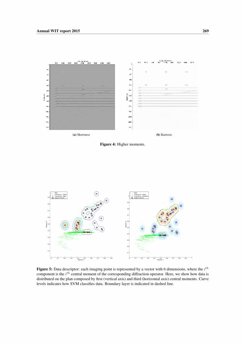
tral moments of the diffraction operator. This vector will play the role of the descriptor in the classificationproblem. On Figures 3(a) and 3(b), it is shown in a gray scale the first and second central moments ofthe section in Figure 1(a). Note that the first moment corresponds to the mean of the diffraction operatoramplitudes, which may generate an scaled version of Kirchhoff imaging. Figures 4(a) and 4(b) show thescaled third and fourth central moments, where noise is significantly suppressed.

Figure 5 shows how imaging points are distributed on cuts of the feature space R6. In order to make


(a) Skewness (b) Kurtosis

Figure 4: Higher moments.

0 0.1 0.2 0.3 0.4 0.5 0.6 0.7 0.8 0.9

0.1

0.2

0.3

0.4

0.5

0.6

0.7

0.8

0.9

Moment :1

Mom

ent :3

Data

Training set − Noise

Training set −Edge

Support Vectors

0 0.1 0.2 0.3 0.4 0.5 0.6 0.7 0.8 0.9 1

0.1

0.2

0.3

0.4

0.5

0.6

0.7

0.8

0.9

1

Moment :1

Mom

ent :3

Data

Training set − Noise

Training set −Reflection

Support Vectors

Figure 5: Data descriptor: each imaging point is represented by a vector with 6 dimensions, where the ith

component is the ith central moment of the corresponding diffraction operator. Here, we show how data isdistributed on the plan composed by first (vertical axis) and third (horizontal axis) central moments. Curvelevels indicates how SVM classifies data. Boundary layer is indicated in dashed line.


sA sB sC sD sE sF0

0.5

1

1.5

2

2.5

3

Sample scatterers

Dis

tan

ce

Similar scatterers

Moments

Diffraction Operator

(a)

dA dB dC dD dE dF dG dH dI1

1.5

2

2.5

3

3.5

4

4.5

5

5.5

Sample scatterers

Dis

tan

ce

Different scatterers

Moments

Diffraction Operator

(b)

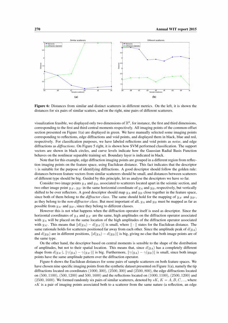
Figure 6: Distances from similar and distinct scatterers in different metrics. On the left, it is shown thedistances for six pairs of similar scatters, and on the right, nine pairs of different scatterers.

visualization feasible, we displayed only two dimensions of R6, for instance, the first and third dimensions,corresponding to the first and third central moments respectively. All imaging points of the common-offsetsection presented on Figure 1(a) are displayed in green. We have manually selected some imaging pointscorresponding to reflections, edge diffractions and void points, and displayed them in black, blue and red,respectively. For classification purposes, we have labeled reflections and void points as noise, and edgediffractions as diffractions. On Figure 5 right, it is shown how SVM performed classification. The supportvectors are shown in black circles, and curve levels indicate how the Gaussian Radial Basis Functionbehaves on the nonlinear separable training set. Boundary layer is indicated in black.

Note that for this example, edge diffraction imaging points are grouped in a different region from reflec-tion imaging points on the feature space, using Euclidean distance. This fact indicates that the descriptorγ is suitable for the purpose of identifying diffractions. A good descriptor should follow the golden rule:distances between feature vectors from similar scatterers should be small, and distances between scatterersof different type should be big. Guided by this principle, let us analyse the descriptors we have so far.

Consider two image points yA and yB , associated to scatterers located apart in the seismic section, andtwo other image point yA′ , yB′ in the same horizontal coordinate of yA and yB , respectively, but verticallyshifted to be over reflectors. A good descriptor should map yA and yB close together in the feature space,since both of them belong to the diffractor class. The same should hold for the mapping of yA′ and yB′ ,as they belong to the non-diffractor class. But most important of all, yA and yB must be mapped as far aspossible from yA′ and yB′ , since they belong to different classes.

However this is not what happens when the diffraction operator itself is used as descriptor. Since thehorizontal coordinates of yA and yA′ are the same, high amplitudes on the diffraction operator associatedwith yA will be placed on the same location of the high amplitudes of the diffraction operator associatedwith yA′ . This means that ‖d(yA) − d(yA′)‖ is small, where ‖ · ‖ states for the Euclidean distance. Thesame rationale holds for scatterers positioned far away from each other. Since the amplitude peak of d(yA)and d(yB) are in different positions, ‖d(yA)− d(yB)‖ is big, giving no clue that both image points are ofthe same type.

On the other hand, the descriptor based on central moments is sensible to the shape of the distributionof amplitudes, but not to their spatial location. This means that, since d(yA) has a completely differentshape from d(yA′), ‖γ(yA) − γ(yA′)‖ is big. Furthermore, ‖γ(yA) − γ(yB)‖ is small, since both imagepoints have the same amplitude pattern over the diffraction operator.

Figure 6 shows the Euclidean distances for some pairs of sample scatterers on both feature spaces. Wehave chosen nine specific imaging points from the synthetic dataset presented on Figure 1(a), namely the tipdiffractions located on coordinates (1000, 300), (2500, 300) and (2500, 800), the edge diffractions locatedon (500, 1100), (500, 1200) and 500, 1600) and the reflections located on (1000, 1100), (2500, 1200) and(2500, 1600). We formed randomly six pairs of similar scatterers, denoted by sK, K = A,B,C, ..., wheresK is a pair of imaging points associated both to a scatterer from the same nature (a reflection, an edge


diffraction or a tip diffraction), and nine pairs of different scatterers, denoted by dK, K = A,B,C...,where dK is a pair of imaging points associated to different scatterers each. Note that similar scatterers arecloser in γ, and different scatterers are more distant in γ, showing that the descriptor γ formed by momentsis more representative in this sense than d, the diffraction operator itself used as the descriptor.

In supervised classifiers, the training set is a subset of feature space. This means that to use the wholediffraction operator as input, for each common-offset section analyzed by the algorithm, the training setmust be generated according to the section geometry. This is a big disadvantage in the sense of classificationtask, since it would be more interesting if one could use the same training set for several data sets to beclassified, regardless of their number particular number of traces. Associated with the fact that diffractionoperator can achieve very big dimensions, it makes the task of building a good training set more challengingin approach of Figueiredo et al. (2013).

Workflow

Our workflow consists mainly on four steps. Pre-processing includes seismic treatments, which may varydepending on the nature of the dataset; velocity model building and ray tracing; and amplitudes pickingalong traveltimes trajectories, to build a cube of amplitudes. The next step consists of filtering of thecube sections, in order to remove undesirable peaks. Depending on your imaging purpose, filtering can beperformed in many ways. With the dataset properly prepared, the next step is the feature space building,that consists on extracting statistical attributes from the cube of amplitudes, and building a vector spacewhere each dimension represents an attribute. Finally, classification is performed, and the last step consistson selecting the best product for interpretation.

Pre-processing

Pre-processing of data must be taken with special care when dealing with seismic diffractions, due to theirsmall amplitudes. Since signal strength of a diffracted wave has rapid decayment with the distance from thetangential portion with the reflected wave, it is common practice to apply a special type of gain, obtained bydividing traces by their envelopes, using a regularization parameter (Landa et al., 1987; Figueiredo et al.,2013). This is the same as obtaining the cosine of the phase of the signal.

The next step consists on building a velocity model to compute traveltimes. This can be done byseveral methods (see Jones, 2010), in time or depth domain. It is typically an iterative process and requiresmany runs of computationally intensive prestack depth migration. To produce accurate images of smallstructures using the method proposed here, it is necessary to build a sufficiently good velocity model, inorder to correctly predict the kinematics of the diffractions.

Our method is presented for a single common-offset section, although the idea can be applied for othergeometries, with appropriate adjustments. Each imaging point is seen as a point scatterer. Once traveltimetable is available, amplitudes along diffraction curves for all imaging points are collected, leading to theconstruction of a cube of amplitudes, with dimensions NX × NZ × NTR, where NX and NZ arehorizontal and vertical dimensions of velocity model, respectively, and NTR is the number of traces ofinput data.

For each vertical profile on a common-offset section, collecting amplitudes along the diffraction curved(y), and displaying it on the corresponding depth, generates a gather where diffraction operators areanalyzed. It might be seen as a slice of the cube of amplitudes normal to NX direction. Tabti et al.(2004) presented some examples of those sections. Correlating with NMO corrected CMP gathers idea, wepropose to call these sections as Diffraction Corrected Common-Offset gathers, or DC-CO gathers.

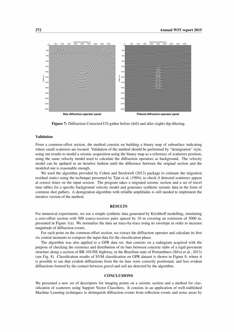
Filtering Note that when a diffraction hyperbola crosses reflection events or other scatterer events in theDC-CO gather, the corresponding diffraction operator has peaks of amplitudes which are not related to theimaging point. These peaks are removed by applying dip-filtering on Diffraction Corrected panel. Tabtiet al. (2004) proposes the application of low-pass filtering, which can remove undesirable peaks. On theother hand, it might not be suitable for our purposes since low pass filtering may also destruct the originalpattern of a diffraction operator shape, leading to further misclassification of the imaging point.


0

200

400

600

800

1000

1200

1400

1600

1800

2000

2200

2400

Depth

(m

) 0 500 1000 1500 2000 2500 3000 3500 4000 4500

Horizontal coordinate (m)

Raw diffraction-operator panel

0

200

400

600

800

1000

1200

1400

1600

1800

2000

2200

2400

Depth

(m

)

0 500 1000 1500 2000 2500 3000 3500 4000 4500 Horizontal coordinate (m)

Filtered diffraction-operator panel

Figure 7: Diffraction Corrected CO gather before (left) and after (right) dip-filtering.

Validation

From a common-offset section, the method consists on building a binary map of subsurface indicatingwhere small scatterers are located. Validation of the method should be performed by “demigration” style,using our results to model a seismic acquisition using the binary map as a reference of scatterers position,using the same velocity model used to calculate the diffraction operators as background. The velocitymodel can be updated in an iterative fashion until the difference between the original section and themodeled one is reasonable enough.

We used the algorithm provided by Cohen and Stockwell (2013) package to estimate the migrationresidual statics using the technique presented by Tjan et al. (1994), to check if detected scatterers appearat correct times on the input session. The program takes a migrated seismic section and a set of traveltime tables for a specific background velocity model and generates synthetic seismic data in the form ofcommon shot gathers. A demigration algorithm with reliable amplitudes is still needed to implement theiterative version of the method.

RESULTS

For numerical experiments, we use a simple synthetic data generated by Kirchhoff modelling, simulatinga zero-offset section with 500 source-receiver pairs spaced by 10 m covering an extension of 5000 m,presented in Figure 1(a). We normalize the data set trace-by-trace using its envelope in order to increasemagnitude of diffraction events.

For each point on the common-offset section, we extract the diffraction operator and calculate its firstsix central moments to compose the input data for the classification phase.

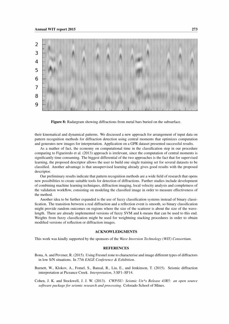
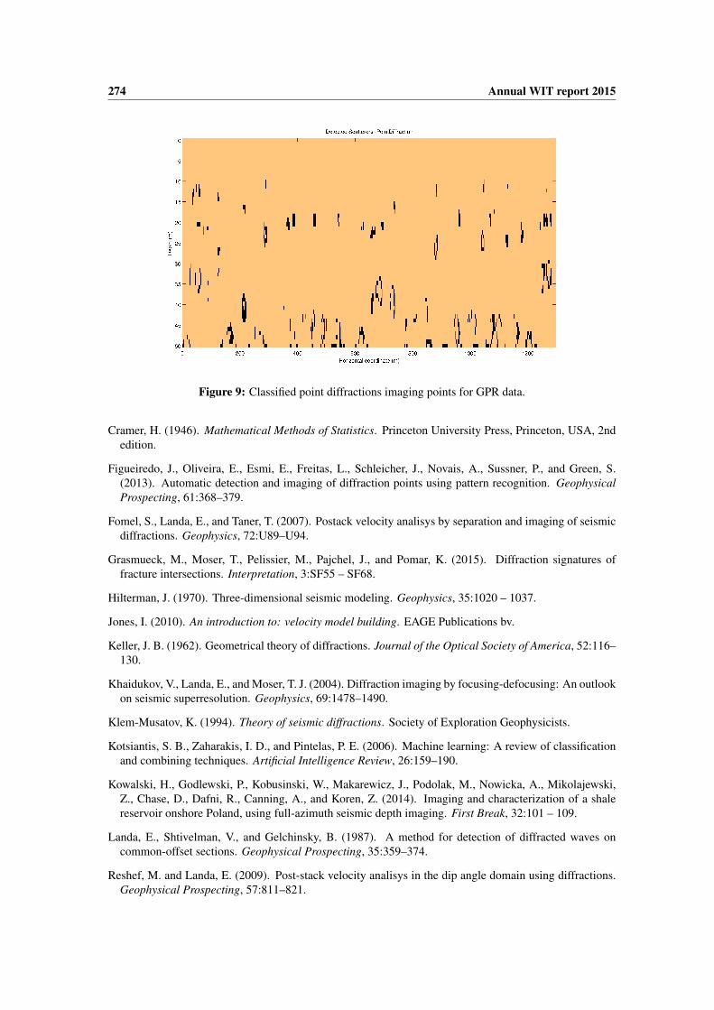
The algorithm was also applied to a GPR data set, that consists on a radargram acquired with thepurpose of checking the existence and distribution of tie bars between concrete slabs of a rigid pavementstructure along a section of BR-101/NE highway, in the Brazilian state of Pernambuco (Silva et al., 2013)(see Fig. 8). Classification results of SVM classification on GPR dataset is shown in Figure 9, where itis possible to see that evident diffractions from the tie bars were correctly positioned, and less evidentdiffractions formed by the contact between gravel and soil are detected by the algorithm.

CONCLUSIONS

We presented a new set of descriptors for imaging points on a seismic section and a method for clas-sification of scatterers using Support Vector Classifiers. It consists in an application of well-stablishedMachine Learning techniques to distinguish diffraction events from reflection events and noise areas by


Figure 8: Radargram showing diffractions from metal bars buried on the subsurface.

their kinematical and dynamical patterns. We discussed a new approach for arrangement of input data onpattern recognition methods for diffraction detection using central moments that optimizes computationand generates new images for interpretation. Application on a GPR dataset presented successful results.

As a mather of fact, the economy on computational time in the classification step in our procedurecomparing to Figueiredo et al. (2013) approach is irrelevant, since the computation of central moments issignificantly time consuming. The biggest differential of the two approaches is the fact that for supervisedlearning, the proposed descriptor allows the user to build one single training set for several datasets to beclassified. Another advantage is that unsupervised learning already gives good results with the proposeddescriptor.

Our preliminary results indicate that pattern recognition methods are a wide field of research that opensnew possibilities to create suitable tools for detection of diffractions. Further studies include developmentof combining machine learning techniques, diffraction imaging, local velocity analysis and completness ofthe validation workflow, consisting on modeling the classified image in order to measure effectiveness ofthe method.

Another idea to be further expanded is the use of fuzzy classification systems instead of binary classi-fication. The transition between a real diffraction and a reflection event is smooth, so binary classificationmight provide random outcomes on regions where the size of the scatterer is about the size of the wave-length. There are already implemented versions of fuzzy SVM and k-means that can be used to this end.Weights from fuzzy classification might be used for weightning stacking procedures in order to obtainmodified versions of reflection or diffraction images.

ACKNOWLEDGMENTS

This work was kindly supported by the sponsors of the Wave Inversion Technology (WIT) Consortium.

REFERENCES

Bona, A. and Pevzner, R. (2015). Using Fresnel zone to characterise and image different types of diffractorsin low S/N situations. In 77th EAGE Conference & Exhibition.

Burnett, W., Klokov, A., Fomel, S., Bansal, R., Liu, E., and Jenkinson, T. (2015). Seismic diffractioninterpretation at Piceance Creek. Interpretation, 3:SF1–SF14.

Cohen, J. K. and Stockwell, J. J. W. (2013). CWP/SU: Seismic Un*x Release 43R5: an open sourcesoftware package for seismic research and processing. Colorado School of Mines.


Figure 9: Classified point diffractions imaging points for GPR data.

Cramer, H. (1946). Mathematical Methods of Statistics. Princeton University Press, Princeton, USA, 2ndedition.

Figueiredo, J., Oliveira, E., Esmi, E., Freitas, L., Schleicher, J., Novais, A., Sussner, P., and Green, S.(2013). Automatic detection and imaging of diffraction points using pattern recognition. GeophysicalProspecting, 61:368–379.

Fomel, S., Landa, E., and Taner, T. (2007). Postack velocity analisys by separation and imaging of seismicdiffractions. Geophysics, 72:U89–U94.

Grasmueck, M., Moser, T., Pelissier, M., Pajchel, J., and Pomar, K. (2015). Diffraction signatures offracture intersections. Interpretation, 3:SF55 – SF68.

Hilterman, J. (1970). Three-dimensional seismic modeling. Geophysics, 35:1020 – 1037.

Jones, I. (2010). An introduction to: velocity model building. EAGE Publications bv.

Keller, J. B. (1962). Geometrical theory of diffractions. Journal of the Optical Society of America, 52:116–130.

Khaidukov, V., Landa, E., and Moser, T. J. (2004). Diffraction imaging by focusing-defocusing: An outlookon seismic superresolution. Geophysics, 69:1478–1490.

Klem-Musatov, K. (1994). Theory of seismic diffractions. Society of Exploration Geophysicists.

Kotsiantis, S. B., Zaharakis, I. D., and Pintelas, P. E. (2006). Machine learning: A review of classificationand combining techniques. Artificial Intelligence Review, 26:159–190.

Kowalski, H., Godlewski, P., Kobusinski, W., Makarewicz, J., Podolak, M., Nowicka, A., Mikolajewski,Z., Chase, D., Dafni, R., Canning, A., and Koren, Z. (2014). Imaging and characterization of a shalereservoir onshore Poland, using full-azimuth seismic depth imaging. First Break, 32:101 – 109.

Landa, E., Shtivelman, V., and Gelchinsky, B. (1987). A method for detection of diffracted waves oncommon-offset sections. Geophysical Prospecting, 35:359–374.

Reshef, M. and Landa, E. (2009). Post-stack velocity analisys in the dip angle domain using diffractions.Geophysical Prospecting, 57:811–821.


Sava, P., Biondi, B., and Etgen, J. (2005). Wave-equation migration velocity analisys by focusing diffrac-tions and reflections. Geophysics, 70:U19–U27.

Schleicher, J., Hubral, P., Tygel, M., and Jaya, M. S. (1997). Minimum aperutres and Fresnel zones inmigration and demigration. Geophysics, 62:183–194.

Silva, L. A., Borges, W. R., Cunha, L. S., Branco, M. G. C., and Farias, M. M. (2013). Use of GPRto identify metal bars and layer thickness in a rigid pavement. Geotechnical and Geophysical SiteCharacterization 4, pages 1341–1346.

Sturzu, I., Popovici, A., Pelissier, M., Wolak, J., and Moser, T. (2014). Diffraction imaging of the EagleFord shale. First Break, 32:49–59.

Tabti, H., Gelius, L., and Hellmann, T. (2004). Fresnel aperture prestack depth migration. First Break,22:39–46.

Theodoridis, S. and Koutroumbas, K. (2009). Pattern Recognition. Academic Press Elsevier, San Diego,USA.

Tjan, T., Lamer, K., and Audebert, F. (1994). Prestack migration for residual statics estimation in complexmedia. SEG Annual Meeting Abstracts.

Trorey, A. W. (1970). A simple theory for seismic diffractions. Geophysics, 35:762–784.

a set of descriptors for automatic classification of

Documents