a semismooth newton-cg method for … semismooth newton-cg method for constrained parameter...

A SEMISMOOTH NEWTON-CG METHOD FOR CONSTRAINEDPARAMETER IDENTIFICATION IN SEISMIC TOMOGRAPHY

CHRISTIAN BOEHM∗ AND MICHAEL ULBRICH†

Abstract. Seismic tomography is a technique to determine the material properties of the Earth’ssubsurface based on the observation of seismograms. This can be stated as a PDE-constrained op-timization problem governed by the elastic wave equation. We present a semismooth Newton-PCGmethod with a trust-region globalization for full-waveform seismic inversion that uses a Moreau-Yosida regularization to handle additional constraints on the material parameters. We establishresults on the differentiability of the parameter-to-state operator and analyze the proposed opti-mization method in a function space setting. The elastic wave equation is discretized by a high-ordercontinuous Galerkin method in space and an explicit Newmark time-stepping scheme. The matrix-free implementation relies on the adjoint-based computation of the gradient and Hessian-vectorproducts and on an MPI-based parallelization. Numerical results are shown for an application ingeophysical exploration on reservoir-scale.

Key words. seismic tomography, full-waveform inversion, elastic wave equation, semismoothNewton, Moreau-Yosida regularization

AMS subject classifications. 86-08, 49M15, 90C06, 35L05

1. Introduction. When earthquakes occur, seismic waves are emitted and canbe measured in form of seismograms at receiver locations far away from the source.The velocity of the travelling waves depends on the material and reflections occurat the transition of different layers of rock. Seismic tomography means to infer thematerial structure of the Earth’s subsurface based on the observation of seismic wavesthat spread through the Earth. This poses a challenging inverse problem since dataobservations are usually only available for a small part of the domain.

There are many applications requiring an accurate knowledge of the Earth’s in-terior. For instance, new insights from seismic tomography can be used to explaingeodynamic processes, to identify potential geologic hazards (e.g. landslides or volca-noes) and to support the search for natural resources.

Seismic tomography can be stated as an optimization problem with PDE con-straints where the unknown material parameters are assumed to be spatially hetero-geneous and constant in time. Depending on whether the medium is solid or fluid, thegoverning equation for the propagation of seismic waves is given either by the elasticor the acoustic wave equation, respectively.

A general overview on seismic tomography can be found in [39, 48]. Iterativeinversion methods based on first-order information have been applied to 2d and 3ddatasets on both regional and continental scale [14, 15, 43]. A Newton-CG methodfor the unconstrained parameter identification problem was presented in [10]. Alter-native approaches work in the frequency domain and involve the Helmholtz equation[34, 37]. To the best of our knowledge, few attention has been paid to the analysisof the infinite-dimensional problem. Recently, results on the differentiability of theparameter-to-solution operator have been established independently in [3] and [27] forthe acoustic wave equation.

∗ETH Zurich, Institute of Geophysics, Sonneggstrasse 5, 8092 Zurich, Switzerland([email protected]).†Technische Universitat Munchen, Chair of Mathematical Optimization, Department of Mathe-

matics, Boltzmannstr. 3, 85748 Garching b. Munchen, Germany ([email protected]).

1

2 C. BOEHM AND M. ULBRICH

Most approaches in full waveform tomography do not include additional con-straints on the material parameters in the formulation of the inverse problem. How-ever, there naturally exist physical bounds, for instance, the non-negativity of wavevelocities or the coercivity of the elliptic operator. Moreover, constraints can be usedto address the ill-posedness of the problem by incorporating additional prior knowl-edge into the problem formulation. This is particularly interesting for the case of thejoint inversion for both Lame coefficients λ and µ or, likewise, for the velocities ofcompressional and shear waves. This is known to be a challenging problem [38] andour approach allows to control the deviation of both parameter fields by imposingbounds on the Poisson’s ratio.

We apply the Moreau-Yosida regularization to handle the constraints on the ma-terial parameters. This penalty method leads to an optimality system involving asemismooth operator equation and requires appropriate optimization methods. Tothis end, we propose a semismooth Newton-CG method and a trust-region global-ization strategy. Semismooth Newton-type methods for optimization problems infunction spaces have been studied extensively in [19, 44, 45] and have been appliedto various types of applications, see, for instance, [30] for an optimal control prob-lem governed by the wave equation and [18, 20, 21, 22] for problems involving theMoreau-Yosida regularization.

Efficient inversion methods rely on a scalable code for the simulation of the elasticwave equation. Our parallel implementation utilizes MPI-communication and worksmatrix-free. Moreover, it is not required to solve a linear system during the simulation,since an explicit Newmark time-stepping scheme [26] and a diagonal mass matrixare used. Forward and adjoint simulations are carried out to efficiently computethe reduced gradient and reduced Hessian-vector products that are required by theNewton-CG method.

This paper is organized as follows. In section 2 we analyze the governing equa-tions and establish continuity and differentiability of the parameter-to-state operator.Based on these results we prove the existence of a solution to the regularized inverseproblem and present the semismooth Newton method in section 3. Furthermore, weestablish estimates for the constraint violation of the Moreau-Yosida regularized so-lution. We continue with the discretization of the problem in section 4 and concludewith numerical examples on reservoir scale problems in 2d and 3d in section 5.

2. Analysis of the elastic wave equation.

2.1. Parameterization of the material coefficients. We consider a boundeddomain Ω ⊂ Rd (d = 2, 3) with a smooth boundary and denote the time intervalby I := (0, T ), T > 0. Furthermore, we assume a heterogeneous density ρ and alinear elastic rheology and let f denote the seismic source function. The elastic waveequation is then given by ρutt −∇ · (Ψ : ε(u)) = f on Ω× I,

u(0) = 0, ut(0) = 0 on Ω,(Ψ : ε(u)) · ~n = 0 on ∂Ω× I.

(2.1)

Here, u denotes the displacement field, ε(u) = 12

(∇u+∇uT

)is the strain tensor of

u and Ψ = (Ψijkl) is a fourth-order elastic tensor. We write Ψ : ε(u) for the matrixwith entries

(Ψ : ε(u))ij =

d∑k,l=1

1

2Ψijkl ε(u)kl =

d∑k,l=1

1

2Ψijkl

([ul]xk + [uk]xl

).

SEMISMOOTH NEWTON METHOD FOR SEISMIC TOMOGRAPHY 3

Remark 2.1. The tensor Ψ of elastic moduli has the symmetry properties Ψijkl =Ψjikl = Ψklij , which yields at most 21 independent components for d = 3. Thisgeneral form allows the treatment of anisotropic material. An important special case,however, is a perfectly elastic, isotropic medium. Here, the tensor simplifies to

Ψijkl = λδijδkl + µ(δikδjl + δilδjk), (2.2)

with the Lame parameters λ and µ. In this case we have the relation

vp =√

(λ+ 2µ)/ρ, vs =√µ/ρ, (2.3)

where vp and vs denote the speed of compressional and shear waves [35]. The isotropicelastic wave equation is thus given by: ρutt −∇ · (2µε(u) + λ(∇ · u)I) = f on Ω× I,

u(0) = 0, ut(0) = 0 on Ω,(2µε(u) + λ(∇ · u)I) · ~n = 0 on ∂Ω× I.

(2.4)

Before we continue with the analysis of the state equation, we have to establisha suitable function space setting for the material parameters. Due to the interdepen-dencies of ρ and Ψ, we keep the density fixed and invert for Ψ only. Depending onthe parameterization of the governing equations, the unknown material parameterscan be the Lame parameters, the velocity of compressional and shear waves, furtherelasticity parameters like the bulk modulus or variables that characterize anisotropy.In either case, the unknown parameter field is heterogeneous in space and does notdepend on time. The number of its components is denoted by n. We then split theparameterization of the material into two parts. On the one hand, we use a ref-erence model Ψ ∈ L∞(Ω)d

4

that is based on prior knowledge and captures majordiscontinuities of the material. On the other hand, we consider smooth variations mfrom that reference model, which we seek to determine by solving the inverse prob-lem. We assume a stronger regularity of the variations with m ∈ M := Mn

1 and aHilbert space M1 →→ L∞(Ω) that is compactly embedded in L∞(Ω). The completeparameterization is now given by

Ψ(m) = Ψ + Φm, (2.5)

with a linear function Φ : Rn → Rd4 that maps m to the full elastic tensor.Remark 2.2. Note that we rely on the strong assumption of the compact embed-

ding M →→ L∞(Ω)n in order to show the existence of a solution to the regularizedinverse problem, see Theorem 3.2. It is a common approach in geophysics to param-eterize for smooth variations from a reference model [13, 41, 48] which often onlyvaries in depth. On the other hand, we allow for less regular material in the referencemodel. For problems in global seismology, a suitable reference model based on a prioriknowledge is available, e.g., the Preliminary Reference Earth Model (PREM) [9].

Now, we introduce additional constraints on the set of feasible parameters. Letma,mb ∈ M with ma ≤ 0 < mb. Furthermore, let p ∈ N, ga, gb ∈ Mp

1 with ga ≤ 0 <gb and B ∈ Rp×n. We consider pointwise constraints on the parameters given by

ma ≤ m ≤ mb and gai ≤n∑j=1

bijmj ≤ gbi , i = 1, . . . , p. (2.6)


In order to facilitate the notation, we set nc := n + p, Mc := Mnc1 , ψa := (ma, ga)T ,

ψb := (mb, gb)T and compactly write the set defined by (2.6) with the help of a linearoperator S ∈ L(M,Mc) as

M∞ad :=m ∈ L∞(Ω)n : ψa ≤ Sm ≤ ψb

. (2.7)

By construction, the set M∞ad is a convex, closed and bounded set. Furthermore, it isnonempty since 0 ∈M∞ad . The admissible set is now given by Mad = M ∩M∞ad .

Remark 2.3. We do not necessarily require that 0 ∈M∞ad and could in principleallow for more general bounds ma < mb and ga < gb. However, from an applicationpoint of view, it seems reasonable to assume a feasible reference model, i.e., zeroshould be a feasible parameter variation. On a different note, we could also extendthe analysis to a more general superposition operator Φ, but restrict the presentationto the linear case. Moreover, it is possible to work with different spaces Mi for everycomponent of the parameters as long as they are compactly embedded into L∞(Ω).

From the definition of the feasible set, it is obvious that simple box constraintscan be imposed by choosing B = 0. We conclude this subsection with an example forthe set M∞ad that imposes additional restrictions on the Poisson’s ratio of the material.

Example 2.4. For isotropic material, the Poisson’s ratio ν can be expressed interms of the Lame coefficients as ν(x) = λ(x)/(2(λ(x) + µ(x))) [35]. Since λ and µare positive, lower and upper bounds in the form νa ≤ ν(x) ≤ νb can be rewritten as2νaµ+ (2νa−1)λ ≤ 0 and −2νbµ+ (1−2νb)λ ≤ 0. If we jointly invert for both Lamecoefficients, we can define λ(m) = λ+m1 and µ(m) = µ+m2 with a reference model(λ, µ). Let ν denote the Poisson’s ratio of the reference model. Then the inequalitiescan be rearranged to

(2νa − 1)m1 + 2νam2 ≤ λ (1− νa

ν), (1− 2νb)m1 − 2νbm2 ≤ λ(

νb

ν− 1). (2.8)

Thus, we set p = 2 and

B =

((2νa − 1) 2νa

(1− 2νb) −2νb

), gb =

(λ (1− νa

ν )

λ(νb

ν − 1)

). (2.9)

Assuming that the reference model has a strictly feasible Poisson’s ratio, we obtaingb > 0. Note that we only have upper bounds in (2.8), but using the fact thatν ∈ (0, 1

2 ], we could easily add an (artificial) lower bound by setting ga = ((2νa −1)mb

1 + 2νama2 , (1− 2νb)ma

1 − 2νbmb2)T .

2.2. Existence, uniqueness and regularity of solutions. Now we turn tothe discussion of the elastic wave equation and analyze the existence and regularityof solutions. We set V = H1(Ω)d and H = L2(Ω)d such that V → H = H∗ → V is aGelfand triple. For fixed m ∈M we define the elliptic operator A(m) ∈ L(V, V ∗) by

〈A(m)v, w〉V ∗,V = (Ψ(m) : ε(v), ε(w))L2(Ω)d×d ∀ v, w ∈ V. (2.10)

In the case of isotropic material, (2.10) can be simplified to: ∀ v, w ∈ V :

〈A(m)v, w〉V ∗,V = (λ(m)∇ · v,∇ · w)L2(Ω) + 2 (µ(m) ε(v), ε(w))L2(Ω)d×d . (2.11)

The elastic wave equation can then compactly be written as

E(u,m) = ρutt +A(m)u, u(0) = 0, ut(0) = 0. (2.12)


The variational form of (2.12) reads as follows: For all v ∈ V and a.a. t ∈ I:

〈ρutt(t), v〉V ∗,V + 〈A(m)u(t), v〉V ∗,V = 〈f(t), v〉V ∗,V . (2.13)

For the rest of the paper we require the following assumptions on the material andthe parameterization:

Assumption 1.(A1.1) The density ρ : Ω → R is sufficiently smooth such that ρv ∈ H1(Ω) for all

v ∈ H1(Ω). Furthermore, ρ satisfies 0 < ρa ≤ ρ(x) ≤ ρb a.e. on Ω with somebounds ρa, ρb ∈ R.

(A1.2) There exists a convex, open and bounded set G∞ ⊂ L∞(Ω)n with M∞ad ⊂ G∞and β1, β2 > 0, independent of m, such that

〈A(m)v, v〉V ∗,V + β1 ‖v‖2H ≥ β2 ‖v‖2V ∀ v ∈ V, ∀ m ∈ G∞. (2.14)

Remark 2.5. For d = 2 or d = 3, Assumption (A1.1) is satisfied, for instance,if ρ ∈ W 1,3(Ω) ∩ L∞(Ω). In this case, we have ∇(ρv) = v∇ρ + ρ∇v ∈ L2(Ω) by theembedding H1(Ω) → L6(Ω) and the generalized Holder inequality with 1

p + 1q = 1

2and p = 6, q = 3 or, resp., p =∞, q = 2.

In the case of perfectly elastic, isotropic material, Assumption (A1.2) is satisfied,for instance, if there exist positive lower bounds on both Lame coefficients.

Lemma 2.6. Consider the isotropic elastic wave equation (2.11) and let the setM∞ad , the reference model (λ, µ) and scalars λmin, µmin > 0 be given, such that for allm ∈ M∞ad there holds λ(m) ≥ λmin and µ(m) ≥ µmin a.e. in Ω. Then Assumption(A1.2) is satisfied.

Proof. By construction, there exists an open and bounded neighborhood G∞ ofM∞ad such that λ(m) ≥ λmin/2 > 0, µ(m) ≥ µmin/2 > 0 a.e. in Ω for all m ∈ G∞.Furthermore, by Korn’s inequality (cf. [25]), there exists a constant C > 0 such that

(ε(v), ε(v))L2(Ω)d×d + ‖v‖2L2(Ω)d ≥ C ‖v‖2H1(Ω)d ∀ v ∈ V. (2.15)

Hence, we obtain for all m ∈ G∞ and all v ∈ V :

〈A(m)v, v〉V ∗,V = (λ(m)∇ · v,∇ · v)L2(Ω) + (2µ(m)ε(v), ε(v))L2(Ω)d×d

≥ 1

2λmin (∇ · v,∇ · v)L2(Ω) + µmin (ε(v), ε(v))L2(Ω)d×d

≥ µmin

(C ‖v‖2V − ‖v‖

2H

).

In order to validate (2.14) in the anisotropic case, further physical properties ofthe elastic tensor have to be exploited that could be incorporated into the definitionof the set M∞ad . For a proof we refer to [7]. The following analysis is restricted to theset G∞, because a unique solution to the elastic wave equation does not necessarilyexist outside of this set.

Theorem 2.7. Let m ∈ G∞. Then the elastic wave equation (2.12) possesses aunique solution in the following settings:

(i) For every f ∈ L2(I;H) there exists a unique solution (u, ut) ∈ C(I;V ) ×C(I;H) and the mapping L2(I;H) → C(I;V ) × C(I;H), f 7→ (u, ut) islinear and bounded.

(ii) For every f ∈ L2(I;V ∗) there exists a unique solution (u, ut) ∈ C(I;H) ×C(I;V ∗) and the mapping L2(I;V ∗) → C(I;H) × C(I;V ∗), f 7→ (u, ut) islinear and bounded.


Proof. Since m ∈ G∞, A(m) is uniformly coercive by Assumption (A1.2). Fur-thermore, Assumption (A1.1) ensures the applicability of general results for hyperbolicequations. In fact, (A1.1) yields (ρv, v)H ≥ ρa‖v‖2H for all v ∈ V and the usual energyestimates can be used. Hence, the existence and regularity of a unique solution aswell as the dependence on the right-hand side f follows by standard arguments (cf.Chapter 3, Theorem 8.1, 8.2 and, respectively, Theorem 9.3, 9.4 in [32]).

Note that in order to achieve continuity of the solution in time, a modificationon a set of measure zero might be necessary. The regularity of the solution can beimproved by exploiting a higher temporal regularity of the seismic source.

Theorem 2.8. Let m ∈ G∞ and f ∈ L2(I;V ∗) with f = 0 near t = 0 and,additionally, ft ∈ L2(I;V ∗). Then there exists a unique solution u to the elastic waveequation (2.12) satisfying u ∈ C(I;V ), ut ∈ C(I;H), utt ∈ C(I;V ∗) and the mapping

H1(I;V ∗)→ C(I;V )× C(I;H)× C(I;V ∗), f 7→ (u, ut, utt) (2.16)

is linear and bounded. For fixed f , the set of solutions u(m) ∈ C(I;V ) ∩ C1(I;H) isuniformly bounded for all m ∈ G∞.

Proof. The proof follows the lines of the proof of Chapter 3, Theorem 9.3 for theexistence of very weak solutions in [32]. However, the crucial difference is the improvedregularity in space that is obtained by utilizing the higher temporal regularity of theright-hand side. We consider

fk ∈ H1(I;H) with fk → f in H1(I;V ∗), (2.17)

and the problem

ρ(uk)tt(t) +A(m)uk(t) = fk(t), uk(0) = 0, (uk)t(0) = 0. (2.18)

By formally differentiating with respect to t and substituting (uk)t by wk, we obtain

ρ(wk)tt(t) +A(m)wk(t) = (fk)t(t), wk(0) = 0, (wk)t(0) = 0. (2.19)

Here, we used that f is zero near t = 0. Since (fk)t ∈ L2(I;H), there exists a uniquesolution wk ∈ C(I;V ) ∩ C1(I;H) to (2.19) by Theorem 2.7. We define the auxiliary

function vk(t) :=∫ t

0wk(τ) dτ and obtain

vk ∈ C1(I;V ), (vk)t = wk ∈ C(I;V ), (vk)tt = (wk)t ∈ C(I;H). (2.20)

Integrating (2.19) in time and inserting the homogeneous initial data yields

0 =

t∫0

ρ(wk)tt(τ)+A(m)wk(τ)− (fk)t(τ) dτ = ρ(vk)tt(t)+A(m)vk(t)−fk(t). (2.21)

By subtracting the original equation (2.18) from (2.21), we obtain

ρ(vk−uk)tt(t)+A(m)(vk−uk)(t) = 0, (vk−uk)(0) = 0, (vk−uk)t(0) = 0. (2.22)

Hence, by the uniqueness of the solution due to Theorem 2.7, we obtain uk = vk and(uk)t = wk in [0, T ]. Thus, we have shown that vk is the unique solution to (2.18).The improved regularity in space remains to be shown. In [32], Chapter 3, proof ofTheorem 9.3, the energy estimates

‖(uk)t(t)‖2H + ‖(uk)tt(t)‖2V ∗ ≤ C ‖(fk)t‖2L2(I;V ∗) , (2.23)

‖(uk)(t)‖2H + ‖(uk)t(t)‖2V ∗ ≤ C ‖(fk)‖2L2(I;V ∗) (2.24)


are derived for a.a. t ∈ I. Using (2.14) and Assumption 1, we deduce

β2 ‖uk(t)‖2V ≤ 〈A(m)uk(t), uk(t)〉V ∗,V + β1 ‖uk(t)‖2H= 〈fk(t)− ρ(uk)tt(t), uk(t)〉V ∗,V + β1 ‖uk(t)‖2H (2.25)

≤ (‖fk(t)‖V ∗ + Cρ ‖(uk)tt(t)‖V ∗) ‖uk(t)‖V + β1 ‖uk(t)‖2H≤(‖fk(t)‖V ∗ + c1 ‖(fk)t‖L2(I;V ∗)

)‖uk(t)‖V + c2 ‖(fk)‖2L2(I;V ∗) ,

where we used (2.23) and (2.24) in the last inequality. Next, we use Young’s inequalityto obtain (

‖fk(t)‖V ∗ + c1 ‖(fk)t‖L2(I;V ∗)

)‖uk(t)‖V ≤

1

2β2

(‖fk(t)‖V ∗ + c1 ‖(fk)t‖L2(I;V ∗)

)2

+β2

2‖uk(t)‖2V .

(2.26)

Hence,

β2

2‖uk(t)‖2V ≤

1

2β2

(‖fk(t)‖V ∗ + c1 ‖(fk)t‖L2(I;V ∗)

)2

+ c2 ‖(fk)‖2L2(I;V ∗) . (2.27)

Now, we can estimate ‖fk(t)‖V ∗ ≤ ‖fk‖C(I;V ∗) ≤ c ‖fk‖H1(I;V ∗) by the embedding

H1(I;V ∗) → C(I;V ∗) and finally obtain by combining (2.23) and (2.27):

sup0≤t≤T

(‖uk(t)‖2V + ‖(uk)t(t)‖2H + ‖(uk)tt(t)‖2V ∗

)≤ C ‖fk‖2H1(I;V ∗) . (2.28)

Thus, uk (resp. (uk)t, (uk)tt) remain in a bounded set of L2(I;V ) (resp. L2(I;H),L2(I;V ∗)). We can therefore extract a weakly convergent subsequence uκ u inL2(I;V ) as well as uκ u in H1(I;H) and uκ u in H2(I;V ∗). By the embeddingsH1(I;H) →→ C(I;H) and H2(I;V ∗) →→ C1(I;V ∗), we obtain uκ → u in C(I;H)and (uκ)t → ut in C(I;V ∗). Therefore, 0 = uκ(0) → u(0) in H, i.e., u(0) = 0, and0 = (uκ)t(0)→ ut(0) in V ∗, i.e., ut(0) = 0. Hence, by passing to the limits in (2.18)we find that u is a solution to the elastic wave equation.

The continuous dependence in (2.16) follows from (2.28), cf. Chapter 3, Remark9.11 in [32]. By Assumption (A1.2), all constants are independent of m. Thus, the setof unique solutions u(m) ∈ C(I;V ) ∩ C1(I;H) is uniformly bounded for all m ∈ G∞and fixed f ∈ H1(I;V ∗).

Corollary 2.9. Let F k = Hk(I;V ∗), k ≥ 1, and F k0 ⊂ F k denote the subset ofsource functions with f = 0 near t = 0. Then, for every f ∈ F k0 and fixed m ∈ G∞,there exists a unique solution u ∈ Ck−1(I;V ) ∩Ck(I;H) ∩Ck+1(I;V ∗) to the elasticwave equation (2.12). The mapping

F k0 → Ck−1(I;V ) ∩ Ck(I;H) ∩ Ck+1(I;V ∗), f 7→ u (2.29)

is linear and bounded and for fixed f ∈ F k0 , the set of solutions u(m) ∈ Ck−1(I;V ) ∩Ck(I;H) is uniformly bounded for all m ∈ G∞.

Proof. The proof follows by induction and Theorem 2.8 which gives the casek = 1. Now, assume the statement is true for k ∈ N and let f ∈ F k+1

0 . Similar as inthe proof of Theorem 2.8 we consider

ρ(w)tt +A(m)w = ft, w(0) = 0, wt(0) = 0. (2.30)


By the induction hypothesis there exists a unique solution w ∈ Ck−1(I;V )∩Ck(I;H)∩Ck+1(I;V ∗) to (2.30). Using the auxiliary function v ∈ Ck(I;V ) ∩ Ck+1(I;H) ∩Ck+2(I;V ∗) defined by v(t) =

∫ t0w(τ) dτ and integrating (2.30) in time, we find that

v is the unique solution to

ρvtt +A(m)v = f, v(0) = 0, vt(0) = 0. (2.31)

which concludes the induction step.Remark 2.10. Usually, second-order hyperbolic equations require stronger com-

patibility conditions on the initial values and the right-hand side (cf. §7.2 Theorem6 in [11]) to establish similar results as in Theorem 2.8 and Corollary 2.9. Since wework with homogeneous initial data, these requirements are implicitly given by f = 0near t = 0. Moreover, in this case also the solution to the elastic wave equation iszero near t = 0, which we will frequently use in the following.

In the next step, we establish continuity and Frechet differentiability of theparameter-to-state operator by utilizing a higher temporal regularity of the source.

Theorem 2.11. For all m ∈ G∞ and f ∈ F k+10 , k ≥ 1, the elastic wave

equation defined in (2.12) possesses a unique solution u(m) ∈ Ck(I;V ) ∩ Ck+1(I;H)and m 7→ u(m) is Lipschitz continuous as a map from G∞ to Ck−1(I;V )∩Ck(I;H).

Proof. By Corollary 2.9, there exists a unique solution u(m) ∈ Ck(I;V ) ∩Ck+1(I;H) to (2.12). Let s ∈ L∞(Ω)n satisfy m + s ∈ G∞. Then, again by Corol-lary 2.9, there exists a unique solution u(s) := u(m + s) ∈ Ck(I;V ) ∩ Ck+1(I;H)to E(u(s),m + s) = f and ‖u(s)‖Ck(I;V ) ≤ C uniformly for all s ∈ L∞(Ω)n withm+ s ∈ G∞. We denote the difference by h := u(s)− u(m) and obtain:

0 = E(u(s),m+ s)− E(u(m),m) = ρ(utt(s)− utt(m)) +A(m+ s)u(s)−A(m)u(m)

= ρhtt +A(m)h−A(m)u(s) +A(m+ s)u(s).

Using the notation A∆(s) ∈ L(V, V ∗) for the operator defined by

〈A∆(s)v, w〉V ∗,V = ((Φs) : ε(v), ε(w))L2(Ω)d×d ∀ v, w ∈ V, (2.32)

we obtain A∆(s) = A(m+s)−A(m) and find that h satisfies an elastic wave equation

E(h,m) = −A∆(s)u(s), h(0) = 0, ht(0) = 0. (2.33)

Since u(s) ∈ Ck(I;V )∩Ck+1(I;H), we obtain −A∆(s)u(s) ∈ Ck(I;V ∗) ⊂ Hk(I;V ∗)and, furthermore, −A∆(s)u(s) ∈ F k0 , due to f ∈ F k+1

0 and the homogeneous initialconditions. Hence, we can apply Corollary 2.9 and obtain

‖h‖Ck−1(I;V ) + ‖ht‖Ck−1(I;H) ≤ C1 ‖A∆(s)u(s)‖Hk(I;V ∗)

≤ C2 ‖s‖L∞(Ω)n ‖u(s)‖Ck(I;V ) ≤ C3 ‖s‖L∞(Ω)n .(2.34)

Remark 2.12. Note that it is necessary to exploit a higher temporal regularityof the source term in order to show the continuity (and differentiability) of the stateu(m) with respect to m. In fact, consider f ∈ L2(I;H) and h := u(s) − u(m) as inthe proof of Theorem 2.11. We obtain that h satisfies

E(h,m) = −A∆(s)u(s), h(0) = 0, ht(0) = 0, (2.35)


and ‖A∆(s)u(s)‖L2(I;V ∗) ≤ C‖s‖L∞(Ω)n . Thus, from the estimate for very weaksolutions (cf. Theorem 2.7) we would only get that m 7→ u(m) is continuous as a mapfrom G∞ to C(I;H) ∩ C1(I;V ∗), although u(m) is bounded in the stronger spaceC(I;V ) ∩ C1(I;H). For f ∈ L2(I;V ∗) the situation is even more critical, because inthis case we have u(s) ∈ C(I;H), but A∆(s) ∈ L(V, V ∗).

Theorem 2.13. Let k ≥ 1 and f ∈ F k+20 . Then the solution operator G∞ →

Ck−1(I;V ) ∩ Ck(I;H), m 7→ u(m) is Frechet differentiable.

Proof. Let m ∈ G∞ and s ∈ L∞(Ω)n with m + s ∈ G∞. Similar as in the proofof Theorem 2.11, we define u(s) as the solution to E(u(s),m + s) = f . In order toshow the Frechet differentiability of the parameter-to-state operator we consider thesolution to the linearized state equation d(m, s)

Eu(u(m),m))d(m, s) = −Em(u(m),m) s, (2.36)

i.e., d(m, s) satisfies

ρ dtt(m, s) +A(m)d(m, s) = −A∆(s)u(m), d(m, s)(0) = 0, dt(m, s)(0) = 0, (2.37)

where A∆(s) is defined as in (2.32). In particular, s ∈ L∞(Ω)n 7→ d(m, s) ∈ Ck(I;V )∩Ck+1(I;H) is linear and bounded by Corollary 2.9.

Let r := u(s)−u(m)−d(m, s) denote the remainder term of the Frechet derivative.By combining the elastic wave equations for u(s), u(m) and d(m, s), we deduce

0 = ρ rtt +A(m+ s)u(s)−A(m)(u(m) + d(m, s))−A∆(s)u(m)

= ρ rtt +A(m)r +A∆(s)(u(s)− u(m)).(2.38)

Hence, r satisfies an elastic wave equation E(r,m) = −A∆(s)(u(s) − u(m)) withhomogeneous initial data. With h := u(s) − u(m), we obtain h ∈ Ck+1(I;V ) ∩Ck+2(I;H) and −A∆(s)h ∈ F k+1

0 . Furthermore, by the Lipschitz continuity of thesolution operator as a map from G∞ to Ck(I;V ) ∩ Ck+1(I;H) (cf. Theorem 2.11),we have ‖h‖Ck(I;V ) ≤ C‖s‖L∞(Ω)n . Thus, applying Corollary 2.9 yields the estimate

‖r‖Ck−1(I;V ) + ‖rt‖Ck−1(I;H) ≤ C1 ‖A∆(s)h‖Hk(I;V ∗)

≤ C2 ‖s‖L∞(Ω)n ‖h‖Ck(I;V ) ≤ C3 ‖s‖2L∞(Ω)n .(2.39)

In particular, the remainder term r satisfies

‖r‖Ck−1(I;V ) + ‖rt‖Ck−1(I;H) = o(‖s‖L∞(Ω)n

)for ‖s‖L∞(Ω)n → 0. (2.40)

By further pursuing this technique, we can also establish higher-order Frechetdifferentiability of the solution operator under suitable assumptions on the seismicsource. Here, we will require the following notation. Let s = (s1, . . . , si) be a tupleof length i with sj ∈ L∞(Ω)n, j = 1, . . . , i. Furthermore, for 1 ≤ j ≤ i, we denote bys−j := (s1, . . . , sj−1, sj+1, . . . , si) the (i− 1)-tuple of elements of s except sj .

Theorem 2.14. Let k ≥ 1 and f ∈ F k+20 . Then the solution operator G∞ →

C(I;V )∩C1(I;H), m 7→ u(m) is k-times Lipschitz continuously Frechet differentiableon G∞. Furthermore, let s = (s1, . . . , si) with sj ∈ L∞(Ω)n and m + sj ∈ G∞,j = 1, . . . , i. Then the i-th derivative applied to s is recursively defined as the unique


solution di := di(m, s) to

E(d1,m) = −A∆(s1)u(m), d1(0) = 0, d1t (0) = 0 (i = 1), (2.41)

E(di,m) = −i∑

j=1

A∆(sj) di−1(m, s−j), di(0) = 0, dit(0) = 0 (2 ≤ i ≤ k). (2.42)

Proof. For the sake of brevity and since the same techniques as in the proof ofTheorem 2.13 can be applied, we only provide a sketch of the proof.

First, it can be shown inductively that di ∈ Ck−i+1(I;V ) ∩ Ck−i+2(I;H) isuniquely determined by (2.41), (2.42) and satisfies

∥∥di∥∥Ck−i+1(I;V )

+∥∥dit∥∥Ck−i+1(I;H)

≤ Ci∏

j=1

‖sj‖L∞(Ω)n , 1 ≤ i ≤ k, (2.43)

with a constant C > 0 that depends linearly on f and can be chosen uniformly onG∞. Here, Theorem 2.13 gives the induction basis for i = 1 and the induction step isobtained by applying Corollary 2.9 to the elastic wave equation defined in (2.42).

In a second step, we consider hi(m, si+1, s) := di(m+si+1, s)−di(m, s) with si+1 ∈L∞(Ω)n and m + si+1 ∈ G∞. With h0(m, s1, ∅) := h0(m, s1) := u(m + s1) − u(m),we deduce from (2.41), (2.42) that hi = hi(m, si+1, s) satisfies:

E(hi,m) = −i∑

j=1

A∆(sj)hi−1(m, si+1, s−j)−A∆(si+1)di(m+ si+1, s), (2.44)

and hi(0) = 0, hit(0) = 0. Again, we can show inductively that hi ∈ Ck−i(I;V ) ∩Ck−i+1(I;H) is uniquely determined by (2.44) and satisfies

∥∥hi∥∥Ck−i(I;V )

+∥∥hit∥∥Ck−i(I;H)

≤ Ci+1∏j=1

‖sj‖L∞(Ω)n , 0 ≤ i ≤ k, (2.45)

where the constant C > 0 depends linearly on f and can be chosen uniformly onG∞. In this case, (2.34) gives the induction basis for i = 0 and the induction stepis obtained by applying Corollary 2.9 to the elastic wave equation defined in (2.44).This shows the Lipschitz continuity of di.

As the final step, we have to provide an estimate for the remainder term of thei-th Frechet derivative. To this end, we set ri(m, s) := hi−1(m, si, s−i)− di(m, s). Bycombining (2.42) and (2.44) we obtain the recursive formula for ri = ri(m, s):

E(ri,m) = −i−1∑j=1

A∆(sj)ri−1(m, s−j)−A∆(si)h

i−1(m, si, s−i), (2.46)

and ri(0) = 0, rit(0) = 0. Now, a third induction shows the estimate

∥∥ri∥∥Ck−i(I;V )

+∥∥rit∥∥Ck−i(I;H)

≤ o(‖si‖L∞(Ω)n

) i−1∏j=1

‖sj‖L∞(Ω)n , (2.47)

for ‖s‖L∞(Ω)n → 0. Here, (2.40) gives the induction basis and subsequently applying

Corollary 2.9 to (2.46) yields the induction step.


There are two immediate generalizations of Theorem 2.14:Corollary 2.15. Let k ≥ 1, l ≥ 0 and f ∈ F k+l+2

0 . Then on a neighborhoodG∞ of M∞ad it holds:

1. The solution operator m 7→ u(m) is k-times Lipschitz continuously Frechetdifferentiable as a map from G∞ to Cl(I;V ).

2. The solution operator m 7→ u(m) is (k + 1)-times Lipschitz continuouslyFrechet differentiable as a map from G∞ to Cl(I;H).

We conclude this section with two remarks.Remark 2.16. It is a valid assumption for problems in seismic tomography

to have homogeneous initial conditions and a force term that is zero near t = 0,which means that the simulation starts with the system at rest. In addition, theexcitations at the hypocenter usually last only for a limited time which is significantlyshorter than the traveltimes to the receiver locations in the far field. An extension toinhomogeneous initial data is possible, but beyond the scope of this paper. Moreover,the assumption of a higher temporal regularity of the right-hand side can be validatedsince wavelets are most commonly used to model the time evolution of the seismicsource. Furthermore, we consider point sources in space which require only a slightsmoothing in V ∗ = (H1(Ω)d)∗. The specific setup will be given in Example 3.4.

Remark 2.17. The results of this section can be carried over to the acousticwave equation that describes the propagation of seismic waves in an inviscid fluidmedium. Here, the unknown material parameter is given by the squared velocity ofcompressional waves. Similar results on the Frechet differentiability of the parameter-to-state operator have been established in [3] and [27]. However, both work withstronger assumptions on the right-hand sides, namely f in Hk(I;H) or even Ck(I , H)instead of Hk(I;V ∗), which is advantageous for modeling point sources.

3. Semismooth Newton method.

3.1. Analysis of the seismic inverse problem. Having established the con-tinuity and the differentiability of the parameter-to-state operator, we now turn tothe formulation of the inverse problem. In seismic tomography, data is usually takenfrom several seismic events. We denote the number of seismic sources by ns and as-sume to have a set of source functions fi, i = 1, . . . , ns. Specific assumptions on theregularity of fi will be made later in this section. Furthermore, for every event weassume to have observations on a subdomain Ωδi × I, Ωδi ⊂ Ω and denote the data byuδi ∈ L2(I;L2(Ωδi )

d) ∩H2(I; (H1(Ωδi )d)∗). The seismic inverse problem is given by:

minu∈U,m∈Mad

J(u,m)

s.t. E(ui,m) = fi, ui(0) = 0, (ui)t = 0, i = 1, . . . , ns.(3.1)

Here, u = (u1, . . . , uns)T ∈ U = Uns is a vector of displacement fields and we set

U := L2(I;V ) ∩H1(I;H) ∩H2(I;V ∗). (3.2)

Remark 3.1. Following the analysis of the elastic wave equation in the previoussection, we recall that for a source f ∈ F l+1

0 (I;V ∗) with some l ≥ 0, we obtainu ∈ Cl(I;V ) ∩Cl+1(I;H) ∩Cl+2(I;V ∗) ⊂ U , i.e., the initial conditions make sense.

The cost functional J : U×M → R has the special structure

J(u,m) =

ns∑i=1

Jfit(ui, uδi ) +

α

2‖m‖2M , (3.3)


that consists of the accumulated misfit from all seismic sources and a Tikhonov-typeregularization term with parameter α > 0. The existence of a solution to the seismicinverse problem can be proven in the following setting.

Assumption 2. In addition to Assumption 1, we require:(A2.1) M is a Hilbert space with compact embedding M →→ L∞(Ω)n.(A2.2) Jfit ≥ 0, convex and, with l ≥ 0, there holds for i = 1, . . . , ns:

• either fi ∈ F l0(I;V ∗) and ui ∈ Cl(I;H) 7→ Jfit(ui, uδi ) is continuous,

• or fi ∈ F l+10 (I;V ∗) and ui ∈ Cl(I;V ) 7→ Jfit(ui, u

δi ) is continuous.

Theorem 3.2. Let Assumption 2 hold. Then the seismic inverse problem (3.1)possesses a solution.

Proof. The proof follows by standard arguments, cf. Theorem 1.45 in [24]. Thecompact embedding M →→ L∞(Ω)n is required to show that the elastic wave equa-tion is weakly sequentially continuous.

Due to the unique solvability of the elastic wave equation for fixed m, we replace(3.1) by the reduced problem:

minm∈Mad

J(u(m),m) (P)

where the displacements u(m) = (u1(m), . . . , uns(m))T

solve

E(ui,m) = fi, ui(0) = 0, (ui)t(0) = 0, i = 1, . . . , ns. (3.4)

The reduced cost functional j is defined by

j : G→ R, m 7→ns∑i=1

Jfit(ui(m), uδi ) +α

2‖m‖2M , (3.5)

where G := M∩G∞. The restriction to G is required, because ui(m) is not necessarilywell-defined on the whole space M . We will outline a strategy to circumvent thisdifficulty in Remark 3.13.

By Theorem 3.2, also the reduced seismic inverse problem (P) admits a solution.Frechet differentiability of the reduced cost functional can be established under thefollowing assumptions. Note that in this case the embedding M → L∞(Ω)n is notrequired to be compact.

Assumption 3. In addition to Assumption 1, we require with k ≥ 1:(A3.1) M is a Hilbert space with continuous embedding M → L∞(Ω)n.(A3.2) With l ≥ 0, there holds for i = 1, . . . , ns:

• either fi ∈ F k+l+10 (I;V ∗) and ui ∈ Cl(I;H) 7→ Jfit(ui, u

δi ) is k-times

continuously Frechet differentiable,• or fi ∈ F k+l+2

0 (I;V ∗) and ui ∈ Cl(I;V ) 7→ Jfit(ui, uδi ) is k-times contin-

uously Frechet differentiable.Theorem 3.3. Let Assumption 3 be satisfied for given k ≥ 1. Then the reduced

cost functional j defined in (3.5) is k-times continuously Frechet differentiable on G.Proof. Assumption 3 ensures the applicability of Corollary 2.9 and Corollary 2.15

that provide the unique solvability of the elastic wave equation and the differentiabilityof the parameter-to-state operator from G∞ to Cl(I;V ) or, respectively, Cl(I;H).Thus, due to the embedding M → L∞(Ω)n, the differentiability properties of Jfit andthe regularization term can be carried over to j.

Next, we give a specific example for a typical problem setup and verify Assumption2 and Assumption 3 for it.


Example 3.4. Let M1 = H2(Ω) ∩ H10 (Ω), i.e., we have M1 →→ L∞(Ω) for

d = 2, 3. We assume homogeneous boundary data, since the material at the surfaceis known and we do not want to update the material parameters at the artificialboundaries of the computational domain (cf. section 5). For notational simplicity, weconsider only one seismic event with a source given by

f(x, t) := s(t)F (x), (3.6)

where the time evolution is modeled by the Ricker wavelet s(t) centered at t0 andwith dominant source frequency ω. We assume a point source located at xs ∈ Ω andmodel the geometry of the source by a time-invariant moment tensor applied to asmoothed Dirac measure in V ∗, cf. [33]. The corresponding force vector is denotedby F ∈ V ∗. In order to ensure that f is zero near t = 0, more precisely, that f ∈ F 3

0 ,we smoothly connect s to zero for |t − t0| larger than a threshold. Data is observedaround receiver locations xr1 , . . . , xrp and we set Ωδ =

⋃pj=1Brj where Brj is a small

ball with center xrj . The misfit function is given by

Jfit(u, uδ) =

1

2

∫ T

0

g(t)‖u(t)− uδ(t)‖2L2(Ωδ)d dt. (3.7)

Here, g : [0, T ]→ R is a smooth weighting function that ensures g(τ) = g(T − τ) = 0for τ ∈ [0, ε) and some small ε, i.e. the misfit is only computed in a subinterval of I.With this choice of f and Jfit, Assumption 2 and Assumption 3 are clearly satisfiedwith k = 2 and l = 0.

Remark 3.5. The proper choice of the misfit functional is crucial for the successof the inversion. The L2-misfit is widely used, cf. [10, 34], and suitable for syntheticdata with a small amount of amount of Gaussian noise. We emphasize, however,that there exist more sophisticated misfit criteria separating phase and amplitudeinformation of the seismograms, see, for instance, [13, 29, 46]. Note that differentcriteria can easily be incorporated into the inversion framework, as long as they aresufficiently smooth, cf. Assumption (A3.2).

3.2. Adjoint-based representation of the derivatives. Having establishedthe differentiability of the reduced cost functional, we can use the adjoint approach toefficiently compute the first and second derivatives with respect to m. Note that thedisplacement fields for different seismic events can be separated completely in (3.1).Likewise, the adjoint states can be computed independently. Due to the symmetry ofA and by carefully integrating by parts, we obtain that the adjoint states pi = pi(m)are (very) weak solutions of the adjoint equations

ρ(pi)tt −∇ · (Ψ(m) : ε(pi)) = −g (ui(m)− uδi )1Ωδi

on Ω× I,pi(T ) = 0, (pi)t(T ) = 0 on Ω,

(Ψ(m) : ε(pi)) · n = 0 on ∂Ω× I.(3.8)

The adjoint equation (3.8) can be interpreted as an elastic wave equation backwardsin time with a different right-hand side. Thus, we can apply the results from section 2to establish existence, uniqueness and regularity of the adjoint states. For the adjoint-based representation of j′, we note that Em(u(m),m) s = A∆(s)u(m) and introduce


the form D : L2(I;V )× L2(I;V )→M∗ defined by

D(v, w)(s) =

∫ T

0

〈A∆(s)v(t), w(t)〉V ∗,V dt

=

T∫0

∫Ω

(ε(v)(x, t)⊗ ε(w)(x, t)) :: ((Φs)(x)) dx dt ∀ s ∈M.

(3.9)

Here, we used the notation (a ⊗ b)ijkl = aijbkl and A :: B =∑ijklAijklBijkl for

tensor products. Then the first derivative of j at a given m ∈ G can be expressed by

〈j′(m), s〉M∗,M = α(m, s)M +

ns∑i=1

D(ui(m), pi(m))(s) ∀ s ∈M, (3.10)

where we used the Riesz representation in the first term.Lemma 3.6. Let m ∈ G, uδi ∈ L2(I;L2(Ωδi )

d)×H2(I; (H1(Ωδi )d)∗) and fi ∈ F 3

0 ,i = 1, . . . , ns. Then there exists a unique adjoint state pi(m) ∈ C1(I;V ) ∩ C2(I;H)and pi(m) ∈ C1(I;V ) ∩ C2(I;H) is uniformly bounded for all m ∈ G. Moreover, forany subset G′ ⊆ G that is bounded in M , j′(m) ∈M∗ is uniformly bounded on G′.

Proof. We use a time transformation τ := T − t in order to work with initial timeconditions and drop the index i. By Corollary 2.9, we obtain (u − uδ) ∈ H2(I;V ∗)and the weighting g ensures that the adjoint right-hand side is in F 2

0 . and we de-duce the existence of a unique adjoint state p(m) ∈ C1(I;V ) ∩ C2(I;H). Further-more, since u(m) ∈ U is uniformly bounded on G, the adjoint right-hand side isuniformly bounded in H2(I;V ∗) and hence, also p(m) ∈ C1(I;V ) ∩ C2(I;H) is uni-formly bounded on G. Moreover, for every m in G we obtain for arbitrary s ∈M

|〈j′(m), s〉M∗,M | ≤ α‖m‖M‖s‖M +

ns∑i=1

c‖ui(m)‖L2(I;V )‖pi(m)‖L2(I;V )‖s‖L∞(Ω)n

≤ (α‖m‖M + C)‖s‖M .(3.11)

Thus, j′(m) ∈M∗ is uniformly bounded on any bounded subset G′ ⊆ G .We can also employ the adjoint approach to compute operator-vector products

j′′(m)s for a given perturbation s ∈ M . This can be carried out at the cost of twoadditional simulations per seismic event and requires the following steps:

For every i = 1, . . . , ns:1. Compute a perturbed forward wavefield δsui by solving

E(δsui,m) = −A∆(s)ui(m), δsui(0) = 0, (δsui)t(0) = 0. (3.12)

2. Compute a perturbed adjoint wavefield δspi by solving

E(δspi,m) = −g δsui −A∆(s)pi(m), δspi(T ) = 0, (δspi)t(T ) = 0. (3.13)

Then j′′(m)s is given by: ∀ v ∈M

〈j′′(m)s, v〉M∗,M = α(s, v)M +

ns∑i=1

D(δsui, pi(m))(v) +D(ui(m), δspi)(v). (3.14)

Note that the results from section 2 and Lemma 3.6 can be applied to deduce thatδsui and δspi are uniquely determined and bounded in U .


3.3. Moreau-Yosida regularization. Now we turn to the discussion of theoptimization method and continue to work with the setting of Example 3.4. Theconstraints induced by M∞ad are handled by the Moreau-Yosida regularization. Thismethod is commonly used for state-constrained problems, see e.g. [18, 20, 21]. Forfixed γ ∈ (0,∞) we define the penalized problem

minm∈G

jγ(m) := j(m) + γφ(m), (Pγ)

with the penalty function

φ(m) :=1

2

(‖[Sm− ψb]+‖2L2(Ω)nc + ‖[ψa − Sm]+‖2L2(Ω)nc

). (3.15)

Here, [.]+ is a vector defined pointwise by ([v(x)]+)i = maxvi(x), 0, i = 1, . . . , nc.The first-order optimality conditions for (Pγ) are given by:

j′(m) + γS∗([Sm− ψb]+ − [ψa − Sm]+

)= 0 in M∗. (3.16)

Equivalently, we obtain in variational form

〈j′(m), v〉M∗,M + γ([Sm− ψb]+ − [ψa − Sm]+, Sv

)L2(Ω)nc

= 0 ∀ v ∈M. (3.17)

Lemma 3.7. Let Assumption 3 hold with k ≥ 2. Then the optimality condition(3.16) defines a semismooth operator equation with generalized derivative j′′(m) +γS∗∂D(m)S, where ∂D(m) is the set of all operators of the form L∞(Ω)nc 3 v 7→(gi vi)1≤i≤nc with gi ∈ L∞(Ω), i = 1, . . . , nc, and

gi(x)

= 0 if ψai (x) < (Sm)i(x) < ψbi (x),= 1 if (Sm)i(x) < ψai (x) or (Sm)i(x) > ψbi (x),∈ [0, 1] if (Sm)i(x) = ψai (x) or (Sm)i(x) = ψbi (x).

(3.18)

Proof. We only have to consider the second part since j′(m) is smooth. Bydefinition, we have S : M → Mc → L∞(Ω)nc . Furthermore, [.]+ is semismooth fromLq(Ω)nc to L2(Ω)nc for any q > 2 with a generalized derivative given by (gi)1≤i≤nc(cf. Proposition 4.1 in [19] with a straightforward extension to nc > 1). Since S∗ ∈L(Mc

∗,M∗) and L2(Ω)nc →Mc∗, we deduce that (3.16) is semismooth.

We require the following additional assumption on the constraints.Assumption 4.

(A4.1) Either, M1 →W 1,q′(Ω) holds for some q′ > d,or M1 → C0,β(Ω) with 0 < β ≤ 2 and m = 0 on ∂Ω for all m ∈M .

(A4.2) There exist ψ ∈ R and m ∈M such that ψai (x) ≤ 0 < ψ ≤ (Sm)i(x) < ψbi (x)a.e. in Ω for all i = 1, . . . , nc.

Theorem 3.8. Let Assumption 2 and Assumption 3 hold with k ≥ 2 and, addi-tionally, let Assumption (A4.1) be satisfied. Furthermore, let C∞ ⊂ G∞ be a closed,convex set containing a neighborhood of M∞ad . Then, there exists γ0 > 0 such thatthe Moreau-Yosida regularized problem (Pγ) has a solution mγ for all γ > γ0. Fur-thermore, (mγ)γ≥γ0 is bounded in M and all weak limit points of (mγ)γ≥γ0 solve theseismic inverse problem (P).

Proof. First, we show that there exists γ0 > 0 and a closed and convex set C ⊂ Gthat is bounded in M with 0 ∈ C and such that for all γ ≥ γ0:

jγ(m) ≥ jγ0(m) > jγ0(0) = j(0) = jγ(0) ∀ m ∈ G \ C.


This will guarantee the existence of a solution mγ ∈ C to (Pγ) in for all γ ≥ γ0 aswell as the boundedness of (mγ)γ≥γ0 in M . Since 0 ∈M∞ad , we have

jγ(0) =1

2

ns∑i=1

Jfit(ui(0), uδi ) =: J0 ≥ 0, (3.19)

and with ε :=√

2J0/α and Bε(0) := m ∈M : ‖m‖M ≤ ε, we set C := C∞ ∩Bε(0).Next, we prove that there exists γ0 > 0 such that jγ0(m) > jγ0(0) = J0 for allm ∈ G \ C. If this does not hold, then there exist sequences (γk)k∈N with γk → ∞and (mk)k∈N ⊂ Bε(0) \ C∞ with

α

2‖mk‖2M + γkφ(mk) ≤ jγk(mk) ≤ J0 ∀ k ∈ N, (3.20)

where we already used the fact that jγk(m) ≥ α2 ‖m‖

2M > J0 for m /∈ Bε(0). Thus,

(mk)k∈N is bounded in M . Furthermore, (3.20) yields φ(mk) → 0 and for v+k :=

[Smk − ψb]+ + [ψa − Smk]+, we deduce∥∥v+k

∥∥L2(Ω)nc

→ 0. Moreover, (Smk)k∈N is

bounded in Mc and by Assumption (A4.1) also bounded in W 1,q′(Ω)nc with q′ > d or,respectively, bounded in C0,β(Ω)nc with 0 < β ≤ 2. Hence, v+

k is either bounded in

W 1,q′(Ω)nc or in C0,β(Ω)nc . Now, an interpolation inequality between L2(Ω) and ei-ther W 1,q′(Ω) (cf. Theorem 5.10 in [1]) or C0,β(Ω) (cf. Proposition 2.11 in [23]) yields∥∥v+k

∥∥L∞(Ω)nc

→ 0. Thus, mk ∈ C∞ for k sufficiently large. This is a contradiction.

Hence, we can restrict the analysis to the set C ⊂ G and γ ≥ γ0 sufficientlylarge. By construction, A(m) is uniformly coercive for all m ∈ C. φ is convex andcontinuous, hence, jγ is weakly lower semi-continuous and the existence of a solutionmγ ∈ C to the regularized problem (Pγ) follows again by standard arguments. Now,let m be a solution to the seismic inverse problem (P). By the optimality of mγ for(Pγ), we obtain:

α

2‖mγ‖2M ≤ j(mγ) ≤ j(mγ) + γφ(mγ) = jγ(mγ) ≤ jγ(m) = j(m). (3.21)

Since (mγ)γ≥γ0 is bounded in M , there exist weak limit points. Moreover, (3.21)yields that γφ(mγ) is uniformly bounded for all γ > 0 and, hence, φ(mγ) → 0 forγ →∞. Now, consider a weak limit point m∗ and a sequence (γk)k∈N with mγk m∗.Due to the compact embedding M →→ L∞(Ω)n, we have mγk → m∗ in L∞(Ω)n

(and also strong convergence in L2(Ω)n). Since φ(mγk) → 0, we obtain again by aninterpolation inequality

∥∥v+k

∥∥L∞(Ω)nc

→ 0, i.e., m∗ is feasible for (P). It remains to

be shown, that m∗ is a solution to (P). The sequence of optimal function values ofthe penalized problem is monotonically increasing, since

jγk(mγk) ≤ jγk(mγk+1) ≤ jγk+1

(mγk+1). (3.22)

Together with (3.21) this implies that (jγk(mγk))k∈N converges. By the lower semi-continuity of j, we obtain

j(m∗) ≤ lim infk→∞

j(mγk) ≤ lim infk→∞

jγk(mγk) = limk→∞

jγk(mγk) ≤ j(m). (3.23)

Due to the optimality of m, all inequalities above are satisfied with equality. Hence,j(m∗) = j(m) and m∗ solves (P).

We continue to use the notation v+γ = [Smγ −ψb]+ + [ψa − Smγ ]+ and state the

following result concerning the rate of convergence.


Theorem 3.9. Let Assumption 2 and Assumption 3 hold with k ≥ 2, and letAssumption (A4.1) be satisfied with the embedding M1 → W 1,q′(Ω). Furthermore,let (mγk)k∈N be a weakly convergent subsequence with mγk m∗ ∈ M . Then theinfeasibility of solutions mγ to (Pγ) is bounded by

‖v+γk‖L2(Ω)nc = o

(γk− 1

2

)(γk →∞) and (3.24)

‖v+γk‖L∞(Ω)nc = o

(γ−ηk

)with η =

q′ − dq′d+ 2(q′ − d)

. (3.25)

Proof. From (3.21) we obtain

jγk(mγk) = j(mγk) +γk2‖v+γk‖2L2(Ω)nc ≤ j(m), (3.26)

where m solves (P). Hence,

‖v+γk‖2L2(Ω)nc ≤

2

γk(j(m)− j(mγk)) . (3.27)

By Theorem 3.8, m∗ solves (P), hence, j(mγk)→ j(m) which shows

‖v+γk‖L2(Ω)nc = o

(γk− 1

2

). (3.28)

Since (mγk)k∈N is bounded in M , (Smγk)k∈N is bounded in Mc and by Assumption

(A4.1) also bounded in W 1,q′(Ω)nc . Thus, an interpolation inequality yields the L∞-estimate similar to Lemma 8.26 in [45].

Example 3.10. We consider M1 = H2(Ω) ∩ H10 (Ω). Then we have M1 →→

L∞(Ω) and M1 → W 1,q′(Ω) for all q′ with 1 ≤ q′ ≤ 6 (d = 2, 3). Thus, for d = 3 weobtain the estimate

‖v+γk‖L∞(Ω)nc = o

(γ− 1

8

k

). (3.29)

Following the derivation in [23] we obtain alternative estimates using interpolationbetween L1(Ω) and C0,β(Ω).

Theorem 3.11. Let Assumption 2 and Assumption 3 hold with k ≥ 2. Addi-tionally, let Assumption 4 be satisfied with the embedding M1 → C0,β(Ω) and m = 0on ∂Ω for all m ∈ M . Consider a weakly convergent subsequence (mγk)k∈N withmγk m∗ ∈M . Then we obtain the following estimate on the constraint violation:

‖v+γk‖L∞(Ω)nc ≤ Cγ−ηk with η =

β

β + d. (3.30)

Proof. The proof follows from [23], Corollary 2.6, but requires that γkv+γk

is

uniformly bounded in L1(Ω)nc for γk → ∞. In order to show this, we use ψ and mfrom Assumption (A4.2) and define w := mγk− 1

2m. Now we observe for i = 1, . . . , nc:

(Smγk)i(x) ≥ ψbi (x) ⇒ 2

ψ(Sw)i(x) =

2(Smγk)i(x)− (Sm)i(x)

ψ>

(Sm)i(x)

ψ≥ 1,


and

(Smγk)i(x) ≤ ψai (x) ⇒ 2

ψ(Sw)i(x) ≤ − (Sm)i(x)

ψ≤ −1,

where we used ψa ≤ 0 in the second part. By testing (3.16) with w we obtain from(3.17):

‖γkv+γk‖L1(Ω)nc ≤

2

ψ

nc∑i=1

∫Ω

γk(([Smγk − ψb]+)i − ([ψa − Smγk ]+)i

)(Sw)i dx

=2

ψ

([Smγk − ψb]+ − [ψa − Smγk ]+, Sw

)L2(Ω)nc

= − 2

ψ〈j′(mγk), w〉M∗,M .

Now, for γk sufficiently large, we have mγk ∈ C with C ⊂ G as defined in the proofof Theorem 3.8. Hence, j′(mγk) is uniformly bounded on C by Lemma 3.6, and weconclude∣∣∣∣− 2

ψ〈j′(mγk), w〉M∗,M

∣∣∣∣ ≤ c‖w‖M ≤ c(‖mγk‖M +1

2‖m‖M

)≤ C. (3.31)

The rest of the proof follows from Corollary 2.6 in [23].Example 3.12. Again, we consider M1 = H2(Ω) ∩H1

0 (Ω). Hence, we have theembedding M1 → C0,β(Ω) with β = 1

2 for d = 2, 3 and for d = 3 we get the estimate

‖v+γk‖L∞(Ω)n ≤ Cγ

− 17

k . (3.32)

Algorithm 1 Penalty Method

1: Choose γ0 > 0, an initial model minit and ε > 0.2: for k = 0, 1, 2, . . . do3: Solve (Pγ) to a specified tolerance and obtain solution mγk .

4: if∥∥v+γk

∥∥2

L2(Ω)nc< ε then

5: Stop with m = mγk .6: else7: Choose γk+1 > γk and set initial model minit = mγk .8: end if9: end for

In order to solve (3.1), we have to compute solutions to a sequence of penalizedproblems (Pγ) with increasing penalty parameter γ, which is described in Algorithm1. It should be emphasized that due to the non-convexity of the problem, we cannotexpect to attain global solutions of (Pγ). Here, we rely on a good starting point inthe vicinity and a suitable regularization parameter.

Note that in our numerical experiments, we update the penalty parameter quiteaggressively instead of solving (Pγ) for a fixed γ to a high accuracy. In particular,γ is increased when the current iterate is infeasible and when the last step provideda good progress towards optimality of (Pγ). To this end, we choose a reduction ofthe norm of the gradient by half an order of magnitude as criterion. This works wellfor the type of constrained problems we are dealing with in section 5. We emphasize,


however, that more sophisticated strategies on updating γ exist [20]. This would bean interesting field for future research.

Remark 3.13. The Moreau-Yosida regularization does not ensure that m stayswithin the set G during the optimization process. This can yield an operator A(m)that is not uniformly coercive, in which case u(m) is not well-defined. To overcomethis difficulty, we can replace Φ in (2.5) by a nonlinear superposition operator thatutilizes a smooth cutoff function to guarantee that the parameters always remainwithin a certain range and allows us to choose G = M . For details we refer to [4].

3.4. Trust-region Newton-CG method. In the next step, we turn to thediscussion of solving the problem (Pγ) for a fixed penalty parameter γ. We apply atrust-region Newton-CG method to solve (Pγ), i.e., we iteratively compute approxi-mate solutions to the trust-region subproblem

mins∈M

qi(s) :=⟨j′γ(mi), s

⟩M∗,M

+ 12

⟨(j′′(mi) + γS∗HiS)s, s

⟩M∗,M

s.t. ‖s‖M ≤ ∆i.(3.33)

Here mi denotes the current iterate and ∆i the trust-region radius in iteration i and qis a quadratic model function with Hi ∈ ∂D(mi) and ∂D(mi) as defined in Lemma 3.7.The first derivatives j′(mi) and operator-vector products j′′(mi)s are computed usingadjoint-based techniques as outlined above. Instead of the exact second derivativesin (3.33), approximations of the Hessian, e.g. by a Quasi-Newton method, can alsobe used. We compute an approximate solution to (3.33) by the Steihaug conjugategradient method [40]. Here, the inner product induced by the norm of M is usedas preconditioner. The CG iterations are early terminated if one of the followingstopping criteria is met: a direction of negative curvature is encountered, the trustregion radius is exceeded by the current iterate, the relative residual is smaller thana threshold, or a maximum number of CG iterations is reached.

Under a standard regularity condition on Hi in (3.33), local superlinear conver-gence of the semismooth Newton method can be established, provided that the initialmodel m0 is chosen sufficiently close to a solution m, cf. Theorem 2.12 in [24]. Thesuperlinear rate of convergence can be maintained if the generalized Newton systemis solved inexactly, cf. Algorithm 3.16 and Theorem 3.18 in [45]. To this end, werequire the Dennis-More conditions [8], see also Assumption 3.14 in [45]. The regu-larity condition that is required to ensure fast local convergence is hard to verify inpractice, but we will investigate the rate of convergence in section 5.

4. Discretization. In this section, we outline the discretization of the inverseproblem. We apply a continuous high-order finite element method for the spatialdiscretization of the state and an explicit time-stepping scheme, see section 4.1 and4.2. This approach is commonly used in seismic applications, cf. [12, 42]. A high-orderdiscontinuous Galerkin method is described in [49]. Furthermore, we use differentspatial meshes for the state and the material parameters. This is motivated by thefact that the information on the material properties is limited, thus a coarser mesh inthe parameter space prevents an over-parameterization. Additionally, the parametermesh might be adaptively refined based on goal-oriented error estimates [4] or priorknowledge to address the varying amount of information in the data in differentregions of the domain. Using different grids for the state and the parameters requiresto interpolate the parameter values onto the finer state mesh in every iteration.

4.1. Spatial discretization of the state space. We consider two- or three-dimensional shape-regular meshes consisting of quadrilateral or hexahedral cells K


that cover the computational domain Ω. Th = K denotes the finite element meshand h the discretization parameter. Let Qs denote the space of polynomials of degrees in each variable xi, i = 1, . . . , d, on the reference cell Kref = [−1, 1]d. We use theLagrange polynomials of degree s with the collocation points of the Gauss-Lobatto-Legendre (GLL) quadrature rule [26] as basis of Qs. This yields a nodal basis forthe numerical representation of the elements of Qs. Let ξi, i = 0, . . . , s, denote thecollocation points of the GLL rule on the interval [−1, 1]. Furthermore, let li denotethe Lagrange polynomials associated with the points ξi. We obtain the polynomialbasis on the reference cell by tensorization of the 1d bases, i.e, for a multi-indexι ∈ 0, . . . , sd we define

ϕι : Kref → R, ϕι(x) :=

d∏i=1

lιi(xi). (4.1)

By definition, the Lagrange polynomials vanish at all but one of the collocation points.Integrals over the reference cell are approximated by the GLL quadrature rule, whichis exact for integrands in Q2s−1. Now, we introduce the finite element subspacesV sh ⊂ V by

V sh =vh ∈ C(Ω)d

∣∣ vh|K ∈ Qs(K)d ∀ K ∈ Th, (4.2)

where Qs is obtained by bi- or trilinear transformations of the nodal basis defined onthe reference cell in every component. All numerical tests presented in this paper uses = 4. Detailed derivations of the spatial discretization of the elastic wave equationusing this particular choice of test functions and quadrature rule can be found multipletimes in the literature, see, for instance, [6, 13, 28, 42]. Therefore, we just summarizethe outcome. By replacing V by V sh in (2.13), we obtain the Galerkin approximationfor the polynomial basis and compute the integrals with the GLL quadrature rule.With N := dim(V sh ) and a time-dependent coefficient vector u(t) ∈ C2(I)N , thespatially semi-discrete formulation of the wave equation is a system of linear ODEswhich can be written in the following form:

Mutt(t) + Ku(t) = F(t), (4.3)

Here, M ∈ RN×N denotes the mass matrix (modified to include ρ), K ∈ RN×N is thestiffness matrix and F(t) ∈ RN is the semi-discrete force vector. Most importantly,the quadrature rule in combination with the interpolation nodes of the Lagrangepolynomials yields a diagonal matrix M, which allows for an explicit time-steppingscheme. On the other hand, this introduces an integration error, because the GLLquadrature rule is only exact for polynomials up to degree 2s− 1.

4.2. Time discretization. Now, we turn to the temporal discretization of thestate equation. Similar to [36], we apply an explicit Newmark time-stepping schemeto solve (4.3). Let

0 = t0 < t1 < . . . < tnt = T

be a partition of the interval I with constant time increment ∆t = tk − tk−1, k =1, . . . , nt. For the Newmark time-stepping scheme we introduce a set of indepen-dent variables uk,0,uk,1,uk,2 to approximate u(tk),ut(tk) and utt(tk), respectively.


Furthermore, let Fk denote the time-discrete version of F(tk). The fully discreteNewmark system is then given by the update formulas (cf. [6, 26]):

uk+1,2 = −M−1 (Kuk+1,0 − Fk+1) ,

uk+1,0 = uk,0 + ∆tuk,1 +1

2∆t2 uk,2,

uk+1,1 = uk,1 +1

2∆t (uk,2 + uk+1,2) .

(4.4)

This scheme is second-order accurate and conditionally stable, see [26], Chapter 9.Note that M and K are time-invariant since the material parameters do not depend ontime and we do not change the state mesh during the simulation. While M is diagonaland can easily be hold in memory, matrix-vector products Kuk+1,0 are computed onthe fly without assembling the matrix K.

The explicit Newmark time stepping scheme is widely used for the numericalsimulation of seismic wave propagation [6, 13, 28]. Note, however, that other (explicit)time stepping schemes can be used as well. For instance, a five-stage fourth-order low-storage Runge-Kutta method is applied in [49]. We also refer to [31], where the elasticwave equation is discretized by the Crank-Nicolson scheme. A severe drawback ofexplicit time-stepping schemes is the limitation of the step-size by the CFL condition.However, due to the diagonal mass matrix, parallelization can be carried out mucheasier as we do not have to solve a linear system in every time step.

4.3. Spatial discretization of the parameter space. As outlined above,we completely separate the discretization of state and parameter meshes. For theparameter mesh, we also use a continuous Galerkin finite element discretization andintroduce the finite element subspace

Msh =

mh ∈ C(Ω)n

∣∣mh|K ∈ Qs(K)n ∀ K ∈ TMh. (4.5)

Here, TMh denotes the decomposition of Ω for the parameter space. TMh will generallyconsists of larger cells than Th. In all numerical tests, we will use a polynomial degreeof s = 1, i.e., bi- or trilinear elements. We recall the assumption M →→ L∞(Ω)that we required to prove the existence of a solution to the inverse problem in theinfinite-dimensional case. In order to justify the choice of bi- or trilinear elements, wepoint out the regularizing effect of the discretization and the equivalence of all normsfor the finite dimensional problem. This motivates that a discrete H1-type normsuffices in our discrete setting. In all numerical examples, we choose the regularizationterm as the weighted sum of the L2-norm and the H1-seminorm, i.e., the discreterepresentation of

α1‖mi‖2L2(Ω) + α2‖∇mi‖2L2(Ω)d , i = 1, . . . , n.

We use the same ratio α1/α2 to compute the ‖.‖M-norm of discrete coefficient vectors.Typically, α2 is a few magnitudes larger than α1 as the L2-regularization would oftenyield oscillating reconstructions. It is important to note that the costs of computingM−1v for the preconditioner as well as the Riesz representation of the derivativewith respect to the M-inner product are negligible compared to solving a single waveequation. Furthermore, the numerical results neither show oscillating solutions norundesirable artifacts in the reconstruction, which justifies our choice of discretizationfor the parameter space.


5. Numerical examples. In this section, we discuss some aspects of the parallelimplementation and present numerical results for inverse problems in 2d and 3d. Inorder to prevent artificial reflections from the boundaries of the computational domain,we impose the following absorbing boundary conditions at all boundaries except thefree surface, cf. [10],

(Ψ(m) : ε(u)) · ~n = vpρ (ut · ~n)~n+ vsρ (ut − (ut · ~n)~n) . (5.1)

Here, ~n denotes the normal vector pointing outwards of the domain. Depending onthe parameterization, vp and vs can, for instance, be computed using (2.3).

5.1. Implementation. The wave propagation code as well as the optimizationroutines are implemented in C++. Due to the similarities in the discretization, the im-plementation is inspired by the SPECFEM code [36]. There are, however, significantdifferences in the computation of the discrete gradient and Hessian-vector products.We make use of the Epetra data structures of the Trilinos library [17] and utilize thetherein provided MPI-communication. Parallelization is carried out in two stages.Trivially, different seismic events can be simulated in parallel and communication isonly required during a post-processing step to add up the individual contributions tothe cost functional and its derivatives. Moreover, the implementation allows to solvea single event on multiple cores using a spatial partitioning of the computationaldomain and communication with MPI.

Table 5.1 and Table 5.2 present statistics for strong and weak parallel scaling ofa forward simulation of the elastic wave equation in 3d. Here, we consider the sameproblem setup as in section 5.3. The computations are carried out on a Cray XC30supercomputer based on Intel R© Xeon R© E5 processors. Both tables indicate a goodparallel performance.

Table 5.1Strong scaling statistic for a simulation of the elastic wave equation in 3d. Discretization: 8,000

elements in total with 4th-order shape functions, 531,441 degrees of freedom, 4,000 time steps.

#cores 1 2 4 8 16 32 64

#elements / core 8,000 4,000 2,000 1,000 500 250 125#dofs / core 531,441 269,001 136,161 68,921 35,301 18,081 9,261total time (s) 458.7 233.4 122.6 67.6 33.4 16.7 8.29par. efficiency 1.0 0.982 0.935 0.848 0.859 0.859 0.865

Table 5.2Weak scaling statistic for a simulation of the elastic wave equation in 3d. Discretization: 1,000

elements per core with 4th order shape functions, 68,921 degrees of freedom per core, 1,000 timesteps (for all configurations). “Scaling efficiency” of N cores is defined as the ratio of the totalrun-time on 8 cores and the total run-time on N cores.

#cores 8 64 512 4096

#elements 8,000 64,000 512,000 4,096,000#elements / core 1,000 1,000 1,000 1,000

total time (s) 16.7 17.0 17.3 17.9scaling efficiency 1.0 0.979 0.963 0.935

5.2. Joint inversion for both Lame coefficients. In this example, we invertfor both Lame coefficients, λ and µ, simultaneously. Here, we use additional con-straints on the Poisson’s ratio of the material to relate both parameter fields to each


other and to ensure that this quantity remains within reasonable bounds. We referto Example 2.4 for a representation of the constraints.

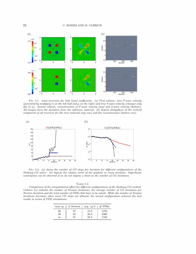
For the test setup, we consider a time interval of 2.5s and a 2d domain of 4km ×4km with a single source in the center. There are 360 receivers on a sphere in 1.2kmdistance from the source. The reference material has a P-wave velocity of 2500m/sand a constant Poisson’s ratio of 0.25. There are four block perturbations of thematerial with a P-wave velocity of either 2750m/s or 2250m/s. These perturbationsare created by modifying either λ or µ, but not both (see first column of Figure 5.1(a)).Thereby, the Poisson’s ratio varies from 0.15 to 0.31. Data is generated by a simulationwith this material model and adding 2% Gaussian noise. The source is modeled bya Ricker wavelet with a dominant frequency of 10Hz. The discretized problem has103,041 spatial grid points for the parameter and state mesh and 3,000 time steps.Note, however, that the material is parameterized with bilinear shape functions whilethe state uses 4th-order polynomials. The initial model is homogeneous with a P-wavevelocity of 2500m/s and a constant Poisson’s ratio of 0.25. We impose constraints onthe Poisson’s ratio for the inverse problem and restrict ν to [0.15, 0.31].

The reconstruction is shown in the second column of Figure 5.1. Here, we showvp and vs computed from the reconstructed λ and µ. The right column in Figure 5.1compares shotgathers of all receivers for the true and reconstructed material. Here,the amplitude of the signal is visualized as a function of receiver’s location (on thehorizontal axis) and time (on the vertical axis). The order of the receivers’ locationsis clock-wise. The first arrival around 0.6s shows the P-wave and the second arrivalat roughly 1s is the S-wave. The wavefronts arrive delayed or premature due to theheterogeneities of the material. In particular, the P-wave arrival time is affected byall four block perturbations, while the S-wave arrival time is only sensitive to the firsttwo. We observe a good match between synthetic and observed data. In particular,the misfit has been reduced by 95% compared to the initial material. Note that theconstraints never become active during the inversion, hence γ is not increased andj and jγ coincide for every iterate. We terminate the Steihaug-CG algorithm if therelative residual is less than

εk = 0.01 ·min1, ‖∇jγ(mi)‖/‖∇jγ(m0)‖,

where mi denotes the i-th Newton iterate. Note that we do not impose a fixed limiton the number of CG iterations in this example. After 22 iterations the norm ofthe gradient has been reduced by more than 12 orders of magnitude and we observea superlinear rate of convergence, see Figure 5.2(b). However, the number of CGiterations increases significantly for the last 7 iterations, see Figure 5.2(a). Therefore,we test different strategies regarding the maximum number of CG iterations anddefine the stopping tolerance as a reduction of the norm of the gradient by 6 ordersof magnitude, which is sufficiently accurate for inverse problems. The computationaleffort is summarized in Table 5.3. With a maximum number of 20 CG iterations, 37Newton iterations are required and the total number of simulations is higher than inthe previous case. Limiting the number of CG iterations to 40 provides a good tradeoff.Here, only two additional Newton iterations are required compared to the unlimitedcase and the total number of PDEs is about 10% less. However, a superlinear rateof convergence cannot be observed for these two configurations, see Figure 5.2(b).Nevertheless, simulating the elastic wave equation dominates the computational costs,thus, the limit of 40 CG iterations gives the best result in terms of computing time.

In order to analyze the effect of constraints in more detail, we modify the prob-lem formulation and restrict ν to values in [0.225, 0.275]. Hence, the true material is


(a) (b)

0 2 40

2

4

0 2 40

2

4

tim

e(s

)

receiver100 200 300

0.5

1

1.5

2

2.5

0 2 40

2

4

0 2 40

2

4

tim

e(s

)

receiver100 200 300

0.5

1

1.5

2

2.5

Fig. 5.1. Joint inversion for both Lame coefficients. (a) First column: true P-wave velocity(generated by modifying λ on the left half and µ on the right) and true S-wave velocity (changes onlydue to µ). Second column: reconstruction of P-wave velocity (top) and S-wave velocity (bottom).All images show the deviation from the reference material. (b) depicts shotgathers of the verticalcomponent of all receivers for the true material (top row) and the reconstruction (bottom row).

(a) (b)

0 5 10 15 20 25 30 35 400

20

40

60

80

100

120

140

160

180

iterations

cg

it

cg 20 cg 40 cg ∞

0 5 10 15 20 25 30 35 4010

−15

10−10

10−5

100

105

iterations

rel. o

ptim

.

cg 20 cg 40 cg ∞

Fig. 5.2. (a) shows the number of CG steps per iteration for different configurations of theSteihaug-CG solver. (b) depicts the relative norm of the gradient in every iteration. Superlinearconvergence can be observed if we do not impose a limit on the number of CG iterations.

Table 5.3Comparison of the computational effort for different configurations of the Steihaug-CG method.

Column 2-4 indicate the number of Newton iterations, the average number of CG iterations perNewton iteration and the total number of PDEs that have to be solved. While the number of Newtoniterations decreases when more CG steps are allowed, the second configuration achieves the bestresults in terms of PDE simulations.

max cg it Newton avg. cg it # PDEs

20 37 15.9 137040 23 20.4 1060∞ 21 25.4 1162


0 2 40

2

4

0 2 40

2

4

0 1 2 3 4

0.16

0.18

0.2

0.22

0.24

0.26

0.28

0.3

0.32

ν

Fig. 5.3. Joint inversion for both Lame coefficients with unattainable true material model. Theleft and middle image depict the reconstructed P-wave (left) and S-wave velocity (middle). Theimage on the right indicates the Poisson’s ratio along the diagonal line depicted in the left image.The plot shows the true material in black, the previous reconstruction in green and the reconstructionwith “hard constraints” in red. Both, lower and upper bounds are active in parts of the domain.

infeasible and the test setup is rather of academic nature. We use the previous recon-struction as initial model and restart the inversion, which required 6 iterations andincluded 2 updates of the penalty parameter. Since the true model is unattainable,the bounds on the Poisson’s ratio become active in the reconstruction and the resultis slightly worse. This is shown in Figure 5.3. The final misfit is 0.0378 comparedto 0.0329 in the first case. Interestingly, however, the reconstructed P- and S-wavevelocities still look very similar with a maximum pointwise difference of 29m/s for vpand 41m/s for vs. This shows that constraints can be used to add prior knowledgeto the formulation of the inverse problem in order to restrict physical quantities thatcannot be resolved by the measurements. The Poisson’s ratio for the true materialand both reconstructions is shown in the right image of Figure 5.3.

5.3. Borehole Tomography in 3D. In this example, we consider a domainof 4km × 4km × 4km and a time interval of 6s. There is one seismic source witha dominant source frequency of 2.5Hz located in the lateral and longitudinal centerat 3.75km depth. There are four boreholes near the corners of the domain equippedwith receivers that measure data every 200m. In addition, there is an array of 441stations near the surface with 21 receivers each in lateral and longitudinal directionsand a 175m spacing. Similar as in the previous example, the “true” material hasa homogeneous P-wave velocity of 2500m/s with two ball-shaped perturbations ofeither 2700m/s or 2250m/s. The material model as well as the locations of sourcesand receivers are shown in Figure 5.4. Here, we assume a constant Poisson’s ratio of0.25 and invert only for λ. Again, the initial model is homogeneous with a P-wavevelocity of 2500m/s. We use the lower and upper bounds of the true material asconstraints on the absolute value of λ, which gives λ ∈ [3.375, 5.042] · 109.

For the spatial discretization of the elastic wave equation, we use 531,441 gridpoints and 4,000 time steps. The parameter mesh has approximately 68,921 degreesof freedom and is discretized by 41 × 41 × 41 grid points. Figure 5.4 shows the re-construction on the right-hand side. Only 6 Newton iterations with a maximum of 40CG steps are required to solve the problem to a relative tolerance of 10−6. Here, themisfit has been reduced by more than 99%. Table 5.4 shows the iteration tableau.Note that this inverse problem is considerably easier to solve than the previous exam-ple. On the one hand, there is only one parameter field to determine instead of bothLame coefficients. On the other hand, there is a good coverage of the domain by thereceivers at the surface and inside the boreholes.


Fig. 5.4. Borehole Tomography. The test setup is shown on the left with black dots representingthe receivers’ locations and the red dot indicating the position of the seismic source. Furthermore,the two perturbations of the true material are visualized and projected to the bottom for a bettervisibility. The right image shows the reconstruction which captures the two perturbations very well.

Table 5.4Iteration tableau for the borehole example. The second column shows the relative decrease of the

objective function and the third column indicates the relative reduction of the optimality criterion.All iterates are feasible.

it rel. obj. rel. optim. cg it

0 1.00 1.001 3.95e-01 7.09e-01 92 4.54e-02 6.04e-02 193 2.25e-02 2.57e-02 404 2.21e-02 5.66e-04 345 2.21e-02 9.34e-06 406 2.21e-02 3.83e-07 40

5.4. 2d elastic inversion with the Marmousi model. The last example isbased on the Marmousi data set provided by the Institut Francais du Petrole EnergiesNouvelles [47]. It consists of a rectangular domain of 9,216m × 3,072m. The wavevelocities are highly heterogeneous and the material contains a series of normal faultsand resulting tilted blocks. Note that the original data set is an acoustic model,however, we generate an elastic model by using the P-wave velocities of the acousticmodel and assuming a constant Poisson’s ratio of 0.25. This gives the relation λ = µand we invert for parameter λ only. Due to the constant Poisson’s ratio the S-wavevelocity is given by vs = (1/

√3)vp. The P-wave velocity profile is depicted in the top

row of Figure 5.5. Here, we only consider the upper part of the domain with up to1km depth, as the reconstruction becomes less accurate for deeper structures.

In our test setup, we place 191 seismic sources at 36m depth and use a Rickerwavelet with a dominant frequency of 5Hz as source time function. 384 receivers thatare placed equidistantly on a horizontal line at 100m depth record the signal (with 1%Gaussian noise added). This setup mimics a marine seismic exploration with sourceslocated in a water layer and geophones measuring data at the seafloor. Note, however,that we do not explicitly model the fluid layer. For the discretized problem we use auniformly refined parameter mesh with 49,665 degrees of freedom. The state equationis discretized with 197,633 degrees of freedom and 6,000 time-steps.


The large number of seismic events makes it computationally very expensive toconsider every seismic source independently. A promising approach is to exploit thelinearity of the elastic wave operator with respect to the displacement field and totrigger the sources simultaneously by building the weighted sum of the individualright-hand sides [16]. In particular, we choose weights wk ∈ Rns , k = 1, . . . ,K, andcompute uk = u(m,wk) by solving the following elastic wave equation for every k:

E(uk,m) =

ns∑i=1

wki fi, uk(0) = 0, ukt (0) = 0. (5.2)

The misfit term in the cost functional compares now the seismograms generated byuk with the weighted sum of the observed data, i.e.,

Jfit

(u(m,wk),

ns∑i=1

wki uδi

), k = 1, . . . ,K. (5.3)

Hence, we only have to consider K (super)-sources instead of ns. In this example,we choose K = 8 and weights wki as i.i.d. samples of Rademacher’s distribution, i.e.,wk ∈ −1, 1ns with P (wki = 1) = P (wki = −1) = 0.5, as has been suggested in [2].

We start the inversion using a reference model that varies only in depth and usesthe average of the true material model in the horizontal plane, see middle row ofFigure 5.5. The reconstructed material is shown in the bottom row of Figure 5.5.Here, the misfit has been reduced by 91%. As stopping criterion we use a relativereduction of the norm of the gradient by either 10−3 or 10−6. The CG iterationsare terminated after at most 40 iterations or if the relative residual is less than 0.01.Table 5.5 summarizes the optimization process for the different tolerances.

1450 1600 1800 2000 2200 2400 m/s

0 2 4 6 8

0

0.5

1dep

th(k

m)

0 2 4 6 8

0

0.5

1dep

th(k

m)

0 2 4 6 8

0

0.5

1dep

th(k

m)

length (km)

Fig. 5.5. P-wave velocity profile of the Marmousi model. Top row: true material, middle row:initial model, bottom row: reconstruction.

In a second step, we additionally enforce lower bounds on the P-wave velocity.In particular, we impose λ ≥ 1.4 · 109 in the whole domain. Due to the constantPoisson’s ratio, this is equivalent (with minor rounding) to vp ≥ 1450[m/s]. This


Table 5.5Computational effort to solve the Marmousi test problem with and without additional con-

straints. The first column indicates the relative tolerance for the stopping criterion.

tolunconstrained constrained

it Newton avg. cg it # PDEs it Newton avg. cg it # PDEs

10−3 24 17.0 7120 25 17.9 780010−6 30 21.6 11104 33 23.3 13112

Table 5.6Iteration tableau for the Marmousi test case with constraints for increasing penalty parameter γ.

γ it Newton avg. cg it # PDEs

1 7 2.4 45610 3 7.0 416102 2 8.0 304103 6 19.2 1992104 15 39.9 9944

bound is only relevant near the surface as the velocities increase with depth andthe true Marmousi model is feasible with respect to this bound. There is a slightimprovement of the reconstruction in shallow depths up to 100m compared to theunconstrained case. Here, the maximum relative error is reduced from 0.22094 to0.22068. The solutions coincide for deeper structures. The number of iterations foran increasing penalty parameter is indicated in Table 5.6. γ is updated as outlined atthe end of section 3.3. Summing up, this test shows a nice application of additionalconstraints, where the solution can be slightly improved by adding prior knowledgeto the problem formulation. More importantly, the computational effort for solvingthe constrained problem does not increase significantly as Table 5.5 indicates.

6. Conclusion. In this paper, we proposed a semismooth Newton method forsolving problems in full-waveform seismic tomography with additional constraints onthe material parameters. We established the continuity and Frechet differentiabilityof the parameter-to-state operator for the elastic wave equation in a suitable func-tion space setting. Constraints on the parameters are treated by the Moreau-Yosidaregularization, which results in a penalized problem, where the first order optimalityconditions are given by a semismooth operator equation. The numerical results un-derline the applicability of the proposed semismooth Newton-PCG method to solveseismic inverse problems in 2d and 3d. A superlinear rate of convergence can beobserved with a suitable stopping tolerance on the CG iterations.

Since the computational costs are vastly dominated by repeatedly solving theelastic wave equation, strategies to reduce the required number of simulations arehighly desirable and an interesting field for future research. For instance, only a subsetof the seismic sources can be used to compute Hessian-vector products. Alternatively,an initial phase using L-BFGS [5] approximations could be incorporated requiringonly 2ns simulations per iterations. Moreover, a preconditioner for the misfit termcan be constructed using the L-BFGS approximation, cf. [10].

Acknowledgements. The authors would like to thank two anonymous refereesand the Associate Editor Tim Kelley for their valuable suggestions that helped toimprove the paper. The authors gratefully acknowledge support by the International


Graduate School of Science and Engineering at the Technische Universitat Munchen,Germany, as well as from the International Research Training Group IGDK1754,funded by the German Science Foundation (DFG). Some of the computations werecarried out on a Linux cluster that was partially funded by the grant DFG INST95/919-1 FUGG.

REFERENCES

[1] R.A. Adams and J.J.F. Fournier. Sobolev Spaces, volume 140 of Pure and Applied Mathematics.Elsevier/Academic Press, Amsterdam, 2003.

[2] A. Aravkin, M. Friedlander, F. Herrmann, and T. van Leeuwen. Robust inversion, dimension-ality reduction, and randomized sampling. Math. Program., 134:101–125, 2012.

[3] K.D. Blazek, C. Stolk, and W.W. Symes. A mathematical framework for inverse wave problemsin heterogeneous media. Inverse Problems, 29(6):065001, 2013.

[4] C. Boehm and M. Ulbrich. A newton-cg method for full-waveform inversion in a coupled solid-fluid system. In Michael Bader, Hans-Joachim Bungartz, and Tobias Weinzierl, editors,Advanced Computing, volume 93 of Lect. Notes Comput. Sci. Eng., pages 99–117. Springer,Berlin, 2013.

[5] R. Byrd, P. Lu, J. Nocedal, and C. Zhu. A limited memory algorithm for bound constrainedoptimization. SIAM J. Sci. Comput., 16(5):1190–1208, 1995.

[6] E. Chaljub, D. Komatitsch, J.-P. Vilotte, Y. Capdeville, B. Valette, and G. Festa. Spectral-element analysis in seismology. In Valerie Maupin Ru-Shan Wu and Renata Dmowska,editors, Advances in Wave Propagation in Heterogenous Earth, volume 48 of Advances inGeophysics, pages 365 – 419. Elsevier, 2007.

[7] S. Dain. Generalized korn’s inequality and conformal killing vectors. Calc. Var. Partial Dif-ferential Equations, 25(4):535–540, 2006.

[8] J. Dennis, Jr. and J. Mor. Quasi-newton methods, motivation and theory. SIAM Rev., 19(1):46–89, 1977.

[9] A.M. Dziewonski and D.L. Anderson. Preliminary reference earth model. Physics of the earthand planetary interiors, 25(4):297–356, 1981.

[10] I. Epanomeritakis, V. Akcelik, O. Ghattas, and J. Bielak. A newton-cg method for large-scalethree-dimensional elastic full-waveform seismic inversion. Inverse Problems, 24(3):034015,2008.

[11] L.C. Evans. Partial Differential Equations. Graduate Studies in Mathematics. AMS, 2010.[12] A. Fichtner. Ses3d version 2.1: Programme description and mathematical background. Tech-

nical report, Ludwig-Maximilians-Universitat Munchen, 2009.[13] A. Fichtner. Full seismic waveform modelling and inversion. Springer, Heidelberg, 2011.[14] A. Fichtner, B.L.N. Kennett, H. Igel, and H.P. Bunge. Theoretical background for continental-

and global-scale full-waveform inversion in the time–frequency domain. Geophys. J. Int.,175(2):665–685, 2008.

[15] A. Fichtner, B.L.N. Kennett, H. Igel, and H.P. Bunge. Full seismic waveform tomography forupper-mantle structure in the Australasian region using adjoint methods. Geophys. J. Int.,179(3):1703–1725, 2009.

[16] E. Haber, M. Chung, and F. Herrmann. An effective method for parameter estimation withpde constraints with multiple right-hand sides. SIAM J. Optim., 22(3):739–757, 2012.

[17] M.A. Heroux, J.M. Willenbring, and R. Heaphy. Trilinos developers guide. Sandia NationalLaboratories, SAND2003-1898, 2003.

[18] M. Hintermuller and M. Hinze. Moreau–yosida regularization in state constrained ellipticcontrol problems: Error estimates and parameter adjustment. SIAM J. Numer. Anal.,47(3):1666–1683, 2009.

[19] M. Hintermuller, K. Ito, and K. Kunisch. The primal-dual active set strategy as a semismoothnewton method. SIAM J. Optim., 13(3):865–888, 2002.

[20] M. Hintermuller and K. Kunisch. Feasible and noninterior path-following in constrained mini-mization with low multiplier regularity. SIAM J. Control Optim., 45(4):1198–1221, 2006.

[21] M. Hintermuller and K. Kunisch. Path-following methods for a class of constrained minimiza-tion problems in function space. SIAM J. Optim., 17(1):159–187, 2006.

[22] M. Hintermuller and K. Kunisch. Pde-constrained optimization subject to pointwise constraintson the control, the state, and its derivative. SIAM J. Optim., 20(3):1133–1156, 2010.

[23] M. Hintermuller, A. Schiela, and W. Wollner. The length of the primal-dual path in moreau–yosida-based path-following methods for state constrained optimal control. SIAM J. Op-


tim., 24(1):108–126, 2014.[24] M. Hinze, R. Pinnau, M. Ulbrich, and S. Ulbrich. Optimization with PDE constraints. Springer,

Berlin, 2008.[25] C. Horgan. Korn’s inequalities and their applications in continuum mechanics. SIAM Rev.,

37(4):491–511, 1995.[26] T.J.R. Hughes. The finite element method. Dover Publications, Mineola, NY, 2000.[27] A. Kirsch and A. Rieder. On the linearization of operators related to the full waveform

inversion in seismology. Math. Methods Appl. Sci., 2013. first published online, doi:10.1002/mma.3037.

[28] D. Komatitsch, C. Barnes, and J. Tromp. Wave propagation near a fluid-solid interface: Aspectral-element approach. Geophysics, 65(2):623–631, 2000.

[29] M. Kristekova, J. Kristek, and P. Moczo. Time-frequency misfit and goodness-of-fit criteria forquantitative comparison of time signals. Geophys. J. Int., 178(2):813–825, 2009.

[30] A. Kroner, K. Kunisch, and B. Vexler. Semismooth newton methods for optimal control of thewave equation with control constraints. SIAM J. Control Optim., 49(2):830–858, 2011.

[31] Axel Kroner. Adaptive finite element methods for optimal control of second order hyperbolicequations. Comput. Methods Appl. Math., 11(2):214–240, 2011.

[32] J.L. Lions and E. Magenes. Non-homogeneous boundary value problems and applications,volume 1. Springer, Berlin, 1972.

[33] R. Madariaga. Seismic source theory. In G. Schubert, editor, Treatise on Geophysics, pages 59– 82. Elsevier, Amsterdam, 2007.

[34] L. Metivier, R. Brossier, J. Virieux, and S. Operto. Full waveform inversion and the truncatednewton method. SIAM J. Sci. Comput., 35(2):B401–B437, 2013.

[35] G. Nolet. A breviary of seismic tomography. Cambridge University Press, Cambridge, 2008.[36] D. Peter, D. Komatitsch, Y. Luo, R. Martin, N. Le Goff, E. Casarotti, P. Le Loher, F. Magnoni,

Q. Liu, C. Blitz, T. Nissen-Meyer, P. Basini, and J. Tromp. Forward and adjoint simulationsof seismic wave propagation on fully unstructured hexahedral meshes. Geophys. J. Int.,186(2):721–739, 2011.

[37] R.G. Pratt, C. Shin, and G.J. Hick. Gauss-newton and full newton methods in frequency-spaceseismic waveform inversion. Geophys. J. Int., 133(2):341–362, 1998.

[38] V. Prieux, R. Brossier, S. Operto, and J. Virieux. Multiparameter full waveform inversionof multicomponent obc data from valhall. part 2 : imaging compressional and shearwavevelocities. Geophys. J. Int., 2013.

[39] N. Rawlinson, S. Pozgay, and S. Fishwick. Seismic tomography: A window into deep earth.Phys. Earth Planet. Int., 178(3-4):101 – 135, 2010.

[40] T. Steihaug. The conjugate gradient method and trust regions in large scale optimization.SIAM J. Numer. Anal., 20(3):626–637, 1983.

[41] C. Tape, Q. Liu, A. Maggi, and J. Tromp. Seismic tomography of the southern california crustbased on spectral-element and adjoint methods. Geophys. J. Int., 180(1):433–462, 2010.

[42] J. Tromp, D. Komatitsch, and Q. Liu. Spectral-element and adjoint methods in seismology.Commun. Comput. Phys., 3(1):1–32, 2008.

[43] J. Tromp, C. Tape, and Q. Liu. Seismic tomography, adjoint methods, time reversal andbanana-doughnut kernels. Geophys. J. Int., 160(1):195–216, 2005.

[44] M. Ulbrich. Semismooth newton methods for operator equations in function spaces. SIAM J.Optim., 13(3):805–841, 2002.

[45] M. Ulbrich. Semismooth Newton Methods for Variational Inequalities and Constrained Opti-mization Problems in Function Spaces. SIAM, Philadephia, PA, 2011.

[46] T. Van Leeuwen and W. A. Mulder. A correlation-based misfit criterion for wave-equationtraveltime tomography. Geophys. J. Int., 182(3):1383–1394, 2010.

[47] R. Versteeg. The marmousi experience: Velocity model determination on a synthetic complexdata set. The Leading Edge, 13(9):927–936, 1994.

[48] J. Virieux and S. Operto. An overview of full-waveform inversion in exploration geophysics.Geophysics, 74(6):WCC1–WCC26, 2009.

[49] L.C. Wilcox, G. Stadler, C. Burstedde, and O. Ghattas. A high-order discontinuous galerkinmethod for wave propagation through coupled elastic-acoustic media. J. Comput. Phys.,229(24):9373 – 9396, 2010.

a semismooth newton-cg method for … semismooth newton-cg method for constrained parameter...

Documents