a search theory of dowry conor walsh
TRANSCRIPT

A Search Theory of Dowry
Conor Walsh
Abstract
Dowries have traditionally been viewed in economics as arising from a supply imbalance
of the marriage market which disadvantages women. In this thesis, a different cause is
proposed. Dowries are modelled as arising from an intertemporal bargaining process in
a frictional search market, with differential aging in favour of men. This extends the in-
sights of the standard model and is able to explain several puzzling stylised facts. Most
notably, dowries may occur when there are more men than women in the market, and
dowry and brideprice can coexist in the same market. The model is extended to include
heterogeneous males of different quality.
Thesis submitted in partial fulfilment
of the requirements of the degree of
Bachelor of International Studies (Honours)
Supervised by Prof. Kunal Sengupta
October 28, 2011
School of Economics
University of Sydney

1
Statement of Originality
I hereby declare that this submission is my own work and to the best of my knowledge
it contains no materials previously published or written by another person, nor mate-
rial which to a substantial extent has been accepted for the award of any other degree or
diploma at University of Sydney or at any other educational institution, except where due
acknowledgement is made in the thesis.
Any contribution made to the research by others, with whom I have worked at University
of Sydney or elsewhere, is explicitly acknowledged in the thesis. I also declare that the
intellectual content of this thesis is the product of my own work, except to the extent that
assistance from others in the project’s design and conception or in style, presentation and
linguistic expression is acknowledged.
SIGNED .........................................................

2
Acknowledgments
This thesis would not be possible without Kunal Sengupta. His patience and skill were
indispensable in all stages of its construction, from conception to completion. This thesis
has also benefited from comments from Abhijit Sengupta and Vladimir Smirnov. The
author is very grateful for their generosity with their time. Thanks also to Andrew Lilley,
Priyanka Goonetilleke and Dominic Reardon for helpful suggestions. Lastly, the author
wishes to thank all his classmates, for their boundless energy, creativity and optimism
which they shared with him at all stages of the Honours year. Of course, all mistakes
contained herein are the fault of the author, and the author alone.

Contents
1 Introduction 41.1 Problems with the Standard Model - Empirical . . . . . . . . . . . . . . . . 41.2 Problems with the Standard Model - Theoretical . . . . . . . . . . . . . . . 51.3 Searching for a Mate . . . . . . . . . . . . . . . . . . . . . . . . . . . . . . . 61.4 Results . . . . . . . . . . . . . . . . . . . . . . . . . . . . . . . . . . . . . . . 7
2 Literature Review 82.1 The Purpose of Dowries . . . . . . . . . . . . . . . . . . . . . . . . . . . . . 8
2.1.1 The Standard Model - Dowry as a Price . . . . . . . . . . . . . . . . 82.1.2 Dowry as a Bequest . . . . . . . . . . . . . . . . . . . . . . . . . . . 92.1.3 Reconciling the two approaches . . . . . . . . . . . . . . . . . . . . . 10
2.2 Central Issues in Dowry Economics . . . . . . . . . . . . . . . . . . . . . . . 102.2.1 Are Dowries Rising? . . . . . . . . . . . . . . . . . . . . . . . . . . . 102.2.2 Why Do Dowries Matter? . . . . . . . . . . . . . . . . . . . . . . . . 11
2.3 Search Costs and Matching . . . . . . . . . . . . . . . . . . . . . . . . . . . 122.3.1 Search Costs and the Marriage Model . . . . . . . . . . . . . . . . . 122.3.2 Dowries and Search Costs . . . . . . . . . . . . . . . . . . . . . . . . 12
3 Theoretical Model 143.1 Solution Concept . . . . . . . . . . . . . . . . . . . . . . . . . . . . . . . . . 15
3.1.1 The Dowry Function . . . . . . . . . . . . . . . . . . . . . . . . . . 163.2 Symmetric Agents . . . . . . . . . . . . . . . . . . . . . . . . . . . . . . . . 173.3 Asymmetric Ageing - Case 1 . . . . . . . . . . . . . . . . . . . . . . . . . . 193.4 Characterizing Asymmetric Equilibria . . . . . . . . . . . . . . . . . . . . . 223.5 Asymmetric Ageing - Case 2 . . . . . . . . . . . . . . . . . . . . . . . . . . 283.6 The Emergence of Dowries . . . . . . . . . . . . . . . . . . . . . . . . . . . . 323.7 A Sufficient Condition for Dowries . . . . . . . . . . . . . . . . . . . . . . . 363.8 Comparative Statics . . . . . . . . . . . . . . . . . . . . . . . . . . . . . . . 39
4 Extension- Heterogeneity of Males 414.1 Generalization to a Continuum of Male Worth . . . . . . . . . . . . . . . . 504.2 A Note on Multiple Searches per Period . . . . . . . . . . . . . . . . . . . . 50
5 Implications of Results 515.1 What Really Causes Dowries? . . . . . . . . . . . . . . . . . . . . . . . . . . 515.2 Empirical Applications . . . . . . . . . . . . . . . . . . . . . . . . . . . . . . 515.3 Banning Dowries- Some Theoretical Insight . . . . . . . . . . . . . . . . . . 525.4 Why Do Dowries Decline With Modernisation? . . . . . . . . . . . . . . . . 53
6 Conclusions 54
A Appendix 56
3

Chapter 1
Introduction
The phenomenon of dowry has long been of interest to social scientists. The practice is
an ancient one- records dating to the 5th Century B.C. describe its occurrence in Ancient
Greece, and later the rising Roman Empire. Its mirror image, brideprice (a payment from
a male to a female at the time of marriage), appears to have an even longer history, being
documented in Ancient Egypt, Mesopotamia and the Incan Empire. As such it is no
mystery that as far back as the 19th Century, it became an object of serious study for
anthropologists and sociologists (Quayle, 1988).
In contrast, it took economists a little longer to embrace this area of study. The first
coherent theoretical framing of the problem arises in the work of Becker (1981) on the
economics of the family. Why it took so long is a little puzzling. Unlike other parts of
Becker’s ground-breaking work in this area (such as the division of labour in a marriage),
physical cash payment from one marital party to another obviously carries an economic
flavour. Perhaps the culprit was the traditional reluctance in economic thought to take
the market to the bedroom (a reluctance which Becker, apparently, never had).
Regardless of this curious blindspot, once the lens of economic analysis was shone on the
problem, open season began. What shall be termed here the ‘standard model of dowries’
was quickly established. This model posits the existence of a ‘marriage market’ operating
in society, where prospective brides and grooms with perfect information will seamlessly
come together in order to form matches, with the aim of maximizing self-gain. Dowry
(or brideprice) will emerge in this market whenever there is an oversupply of brides (or
grooms), in order to equilibrate the demands of both sides.
However, the standard model has not been without problems. They are mentioned here
briefly in two categories, empirical and theoretical, with further analysis undertaken later
in the thesis.
1.1 Problems with the Standard Model - Empirical
If one takes the standard model as correct, then dowry should occur when, for whatever
reason, an imbalance of men and women looking for partners occurs. The women will
4

CHAPTER 1. INTRODUCTION 5
compete on price until those with the highest marginal benefit of marrying exactly equals
the number of available men.
A cursory first glance at the stylized facts of dowry seems to contradict this theory. Some-
what counter-intuitively, dowry seems to occur in modern times in that small subset of
countries where men outnumber women, specifically South Asian countries such as India
and Pakistan. Due to its size, treating India as one country obscures much of interest. If
one looks at the data by region, dowries are shown to be higher in the northern states,
where there are far more men than women (Das Gupta and Bhat, 1997; Dalmia and
Lawrence, 2005).
This fact is well-recognized in the literature, and the response has been to argue that men
and women marry at different ages. Thus, if women begin to marry younger than men,
there may actually be a surplus of eligible women in the marriage market, even when the
gross ratio of females to males is less than one.
However, this has proved unsatisfactory. Even when one does condition cohort size on
marriage ages, the result is that local gender ratios are not empirically significant deter-
minants of dowries. This raises a very fundamental question for adherents to the standard
model of dowries that is often overlooked....just what is causing dowries, if not supply and
demand?1 Can there be dowries when there are more men in the market than women?
Moreover, the standard model seems to rule out entirely the simultaneous occurrence of
dowry and brideprice. In a frictionless market context, the two should engage in a struggle
driven by the rational pursuit of self-gain, and like a battle of matter and anti-matter,
one should eliminate the other. However, it appears that dowry and brideprice may occur
in the same region simultaneously (Murdock, 1967). Murdock documents over a dozen
historical societies which have experienced this concurrence, something which the standard
model lacks an explanation for.
1.2 Problems with the Standard Model - Theoretical
Regardless of the record of the standard model in data, it also retains a somewhat unsat-
isfactory feel. On deeper examination, one cannot escape the conclusion that, except in
the most abstract of senses, there is no such thing as a marriage market. In no society on
Earth is it possible to go to a centralized exchange, view all prospective mates at once,
1Similarly unsatisfactory is an appeal to cultural or historical norms, such as the banal ”to give adowry is simply the custom, nothing more”. Such norms are malleable across time, and should not arise inisolation, without some fundamental behavioural cause. The author rejects this explanation prima facie

CHAPTER 1. INTRODUCTION 6
and then compete with other “buyers” on price to gain a spouse 2.
How does marriage really happen? It may be obvious, but humans devote a considerable
portion of their time and energy to searching for a mate, with search being the operative
word. This process is not perfect- far from it. This author identifies two significant frictions
that operate to the detriment of the searchers. First, search is noncertain, and secondly,
search is nondirected.
Search is said to be noncertain in that the probability of meeting anyone at all (desirable
or not) given a decision to search has been made is not unity. Search is also nondirected,
in that one does not know where one’s perfect match is located. .One may have an idea,
but the process is still inescapably one of screening selected applicants for the desired
attributes.
A true theory of dowry should reflect the way in which individuals look for partners.
1.3 Searching for a Mate
The key question explored in this thesis arises from such an examination, and may be
stated succinctly as, “how do dowries arise in a world where partner search is costly”?
The explanation offered is that, in a developing country context, a woman’s worth may
be declining faster than a man’s with age. In a world where search is costly, this is a
significant asymmetry. If a young woman meets a man and wishes to marry him, in order
to avoid having to go back to the search market as an older woman, she may be willing
to transfer some utility to the man (through a cash payment), and settle now.
It is worthwhile spending some time to justify this assumption, for much depends on
it. Consider the way marriage is modelled by Becker, as a joint production decision to
maximise output. What are the arguments of this function, and what is exactly meant
by output? Becker is refreshingly vague about this point, so here an interpretation will
be offered with specific reference to developing economies, which without exception are
where we observe dowries today. In general, one may imagine that some of the inputs into
a good marriage consist of productive activity- that is, the economic production, domestic
production and child raising undertaken by both parties.
One of the stylized facts about dowries outlined by Anderson (2007a) is that they occur
primarily in traditional societies where women do not take part in agricultural production.
2The reader may well wonder if perhaps something akin to a marriage market exists in the world ofonline dating. After all, it is relatively costless to attain an account at EHarmony.com or Rsvp.com.auand compare and communicate with many potential partners at once. However, anyone with even themost cursory experience with such websites will highlight the informational problems that bedevil them,occasionally leading to their total collapse. While such a topic is profoundly interesting to an economist,it is beyond the scope of this thesis-suffice it to say that Akerlof’s Lemons have electronic counterpartsamong both men and women.
So though they may be increasing in prominence worldwide, this author does not believe that onlinedating websites have fundamentally changed the dating world just yet, and thus will continue on thepresumption that perfect marriage markets are a beautiful abstraction from the real world.

CHAPTER 1. INTRODUCTION 7
This is rather unusual among developing economies, where it is estimated that around 70%
of agricultural work is undertaken by women (FAO, 2011). However, they remain united
with other developing economies in one sense by the fact that women also have very limited
labour market opportunities.
The dearth of both labour market and agricultural opportunities mean that it is conceiv-
able women in dowry-practising countries contribute little in the way of market production
to a household, and instead specialize in domestic production and child rearing. In a sense
(if one can be so crude), women trade children and domestic work with a man in exchange
for the economic resources necessary for survival.
This, however, introduces an asymmetry between men and women. It is a well-established
biological fact that the reproductive ability of women declines much faster then that
of males (see, for example,(Wood, 1989) and (Piette, De Mouzon, Bachelot, and Spira,
1990)). A healthy woman’s most fertile period is from her late teens to her early twenties,
and she becomes, except in rare cases, practically unable to have children around her
forty-fifth birthday. A man, on the other hand, is able to continue conceiving children
well into old age (even though the above papers note a decrease in the quality of sperm).
Therefore, it is likely that an old woman is worth less in a marriage in such developing
countries than a young woman, controlling for mitigating aspects such as looks and wealth,
precisely because her reproductive abilities are lessened and she can produce less children.
But, as a young woman knows she will one day be old, she may pay a man a dowry in
order to marry now. This, it will be shown, provides a powerful explanation for the dowry
phenomenon.
1.4 Results
This thesis demonstrates that such an ageing effect could be a significant determinant of
dowries. It is also demonstrated that dowries can indeed occur when there are more men
than women in the market. Furthermore, it shows that falling search costs are likely to
increase dowries, which has useful implications for policy.
It is further shown in this thesis that brideprice and dowry can coexist in one society. Very
simply, a low quality man and high quality female match can sustain a brideprice, even
if the average dowry paid in the economy is positive, because the cost resulting from the
man rejecting the match in search of a dowry make such an action infeasible. Lastly, it is
demonstrated that older women will pay a higher dowry, and men will on average marry
at an older age than women.
The remainder of the thesis is presented as follows. Chapter 2 reviews the relevant litera-
ture, while Chapter 3 presents the theoretical model. Chapter 4 presents an extension on
the basic model, and Chapter 5 develops some implications of the results obtained.

Chapter 2
Literature Review
2.1 The Purpose of Dowries
In the economic literature, the phenomenon of dowries has typically been studied in two
different conceptual frameworks- as a groom price, the function of which is to clear the
marriage market, or as a bequest to daughters, the function of which is an intergenera-
tional transfer of wealth. These frameworks are entirely distinct and separate manners of
understanding what is occurring when a dowry is paid.
2.1.1 The Standard Model - Dowry as a Price
In Becker’s seminal work on the economics of the family, he modelled marriage as a joint
production decision between a man and a woman to maximise output (both market and
household) (Becker, 1981). One famous result is that in the absence of imperfections, then
the market will exhibit assortative matching (that is, higher quality men will match with
higher quality women). Becker also notes that “this model contrasts sharply with other
models of the marriage market”(ibid, pg 127), such as in Gale and Shapley (1962), as
preferences for partners are not given ex-ante, but emerge ex-post from the equilibrium
generated.
This marriage model also allowed him to construct the first formal statement of the condi-
tions under which dowries may arise. He argued that if the division of output is inflexible,
(that is, determined in some way outside the marriage market, such as through culture, law
or customs), then transfers at marriage should take place to ensure each partner receives
their shadow price.
One intuitive appeal of this explanation for dowries is that it can also be used to explain
brideprices, which have historically been common in Sub-Saharan Africa (Goody and
Tambiah, 1973; Anderson, 2007a), and in parts of rural China and Thailand (Brown,
2009; Cherlin and Chamratrithirong, 1988). A key deficiency of the “Dowry as a Bequest”
approach, outlined below, is that it has no such mirrored and elegant explanation for
brideprices.
8

CHAPTER 2. LITERATURE REVIEW 9
An implication of this is that if there is a surplus of partners on either side of the market,
transfers at marriage should emerge to ensure that the market clears- that it is optimal for
some men or women to remain single with the emergent brideprice/dowry. This concept
is the basis for much of the work in this area (see, for example, (Rajaraman, 1983; Rao,
1993b; Esteve-Volart, 2004; Dalmia, 2004)). It is then important to ask whether this
imbalance based approach is sufficient to explain the phenomenon of dowries in South-
Asia. Firstly, the predominant dowry-generating countries of South Asia such as India
have a highly skewed sex ratio at birth, in favour of men. First documented by Sen
(1990), this is referred to as the “Missing Women” Phenomenon, and has been studied by
a range of disciplines, from economics and demography to anthropology (see, for example,
Johansson and Nygren (1991); Klasen and Wink (2002); Qian (2008)). With time, this
has resulted in unusual population demographics for these countries. For example, the
gross ratio of males to females between the age of 15-64 is 1.06 : 1 for both India and
Pakistan (C.I.A, 2011).
The response has been to argue that because women begin to marry at a younger age
then men, even though the overall ratio of men to women is skewed, there still may be
more women of marriageable age in the market than there are potential husbands. These
hypothesis is known as the “marriage squeeze”. The seminal paper is given by Rao (1993b),
whose asked if dowries are rising with time, and how this might be explained with the
standard model. It is pursued in (Bhat and Halli, 2001) and (Maitra, 2006), among others.
However, the empirical evidence for such a squeeze is mixed, to say the least. If one
looks on a micro-level, it has been shown that local gender ratios are not empirically
significant determinants of dowries (Edlund, 2000; Anderson, 2000; Dalmia and Lawrence,
2005; Arunachalam and Logan, 2006). Factors such as the education levels of the pair,
their respective ages and the wealth and caste of the groom play a much greater role. As
it is probably local ratios that matter more for marriage market dynamics that state or
country-wide ratios, this is a problem with the standard theory of dowries.
2.1.2 Dowry as a Bequest
An alternative to modelling dowries as a price that has been explored extensively in the
literature is viewing dowries as bequests. Their function here is not to clear the marriage
market, but to transfer wealth from one generation to another.
In particular, Botticini and Siow (2003) argue in an influential study that dowries overcome
an important free riding problem in virilocal societies (societies where the son/s will stay
with the family and work with family resources, whereas the daughter will leave the
family). They also posit this as an explanation for why dowries decline in importance with
modernization, which is a well-documented occurrence in the anthropological literature
(Queller and Madden, 1993; Self and Grabowski, 2009). In their model, as development
and labour market opportunities increase for both sons and daughters, there is less instance
of working with the family resources, and thus less of a free-riding problem.

CHAPTER 2. LITERATURE REVIEW 10
Other notable studies of dowry as a bequest include Zhang and Chan (1999) and Suen,
Chan, and Zhang (2003). Zhang and Chan propose that in societies with cultural and
legal barriers to female inheritance of property, dowries play an important role in intra-
generational altruism between parents and daughters, and thus are important tools to
maximise female welfare. Suen et al emphasize that in an altruistic setting, parents are
incentivised to transfer more property to a married child than a single one due to greater
efficiencies in consumption. Such bequests also increase the stability of marriage.
2.1.3 Reconciling the two approaches
Arunachalam and Logan (2006) provide a novel test for which approach is valid for under-
standing the problem. They model an exogenous switching regression for both frameworks
using data from rural Bangladesh, and “find robust evidence of heterogeneity of dowry
motives in the population” (ibid, pg. 27). That is to say, both price and bequest dowry
regimes are present in the data, with dowries as a price being more common, in around
71% of marriage transactions. Moreover, they found that dowries as bequests have de-
creased both in prevalence and magnitude over time, while the incidence of dowries as a
price has increased. Anderson (2000) reveals similar findings for Pakistan.
Using this empirical motivation, this thesis will abstract from dowries which form bequests,
and focus on the price notion.
2.2 Central Issues in Dowry Economics
2.2.1 Are Dowries Rising?
Much of the study of dowries in the economic literature is motivated by inquiry into a
singular phenomenon- whether dowries in South Asia, and especially India, are rising
over time. The original paper by Rao (1993b) suggested that they were, using data from
villages in rural India.
This study spawned a large body of work on dowry inflation. See, for example, (Caldwell,
Reddy, and Caldwell, 1982; Billig, 1992; Rao, 1993a; Maitra, 2006; Sautmann, 2009). All
these studies are attempts (both theoretical and empirical), to account for dowry inflation
using some variant of the marriage squeeze outlined above- where a rising number of
women of marriageable age drives an increase in the dowry level.
However, many of these studies rely on a handful of small and limited datasets. The
difficulty of finding empirical data for marriage transactions in South Asia is well known,
as the practice of dowry has been technically illegal in India since 1961, and is now illegal in
Pakistan and Bangladesh. In practice this has meant that until recently, a comprehensive
investigation into dowry inflation has not been forthcoming.
It is to this end that Arunachalam and Logan (2008) attempted a systematic study of the

CHAPTER 2. LITERATURE REVIEW 11
empirical evidence for rising real dowries. They do not include an estimate of a dowry
function such as in (Rao, 1993b), but use the correlation of the year of marriage with
the real dowry amount (deflated by the price of rice, a method used in the development
literature as standard price indices may not reflect the prices for goods actually used by
the poor (Banerjee and Duflo, 2007)). This simple measure gives them access to a larger
range of datasets from across South Asia. They “do not find any evidence of rising real
dowries” (Arunachalam and Logan, 2008, page 2).
In another interesting study, Edlund attempts to replicate Rao’s results, and is unable to
(Edlund, 2000), though Rao contends that this is because Edlund used a different estimate
of the sex ratio than him (Rao, 2000). Dalmia also attempts to model a hedonic dowry
function with a different dataset, and in doing so, she conclusively rejects the hypothesis
that real dowries in India have been rising with time (Dalmia, 2004).
2.2.2 Why Do Dowries Matter?
Though recent papers have shown that there is mixed evidence for rising dowries, as
Anderson (2007b) notes, this is in one respect a moot point. The evolution of this subfield
of economics has developed new tools and methods for analysing marriage transactions
and has thus advanced the state of scholarly inquiry, regardless of the veracity of the
phenomenon.
This author contends that the concern about rising dowries stems from the same angst
about the phenomenon itself that motivates the entire subfield, and is then in some sense
misguided. The more important question is not whether dowries are rising or falling, but
why they exist in the first place,and what welfare implications they have. This is still an
open scholarly question.
Several recent moves towards the welfare impacts of the practice of dowry deserve to be
noted here. Bloch and Rao (2002) model the incentives towards domestic violence against
women that dowries generate, and find they are significant. The popular press is also
fixated on the violence that notoriously follows dowries, with ‘dowry death’ attracting
widespread outrage and condemnation (Van Willigen and Channa, 1991). In a related
manner, Srinivasan and Bedi (2007) find that the practice of dowry in Southern India is
likely fueling sex-selective abortion and infanticide against baby girls, adding weight to
the urgency of the “Missing Women” phenomenon outlined above. In another intriguing
study, Lahiri and Self (2007) develop a theoretical two-period model which purports that
the practice of dowry, which under Becker’s marriage model may be exacerbated by lack
of opportunities in the labour market for women, can itself lead to more labour market
discrimination, thus entrenching the practice.
An economist may view these facts as evidence that the practice of dowry generates neg-
ative externalities, in that the costs of the decision to marry are not borne entirely by
the bride and groom. The extent and magnitude of these externalities have not been for-
mally studied in the economic literature, and would make an intriguing study. But before

CHAPTER 2. LITERATURE REVIEW 12
this can be done, it is of paramount importance that economists have a coherent model
of dowries which accords both with data and intuition, because a deep understanding of
what is causing the phenomenon is a prerequisite for optimal policy, and even the decision
not to implement any policy at all. It is to this end that we now turn to search models of
marriage.
2.3 Search Costs and Matching
2.3.1 Search Costs and the Marriage Model
The marriage model begun by Becker has been rewritten extensively over the last few
decades to incorporate search costs, following the success this lens of analysis had in the
realm of labour economics.
Smith (2006) extends Beckers work by adapting the marriage model to a world where
search is costly. Smith finds that in the presence of search costs,one can no longer guarantee
positively assortative matching. The intuition is that one be willing to settle for a less
than perfect partner in a frictional market, simply to avoid coming back to the market and
searching again in the future. This work is further developed and formalised in Shimer
and Smith (2000)1. Other novel examples of this literature include Cornelius (2003),
who allows for the possibility of divorce in the marriage market, and Brien, Lillard, and
Stern (2006) which examines household formation and co-residential habitation in a search
framework.
The key to the result by Smith is that search costs as modelled as a cost of time only,
which enter via a discount rate for expected future utility, and the fact that an agent
does not meet every other agent in every period. An alternative approach is to introduce
search costs explicitly, as an additive cost that must be paid in each period that search is
undertaken. A prominent example is Atakan (2006), who constructs a search cost model
of the marriage market with transferable utility and an explicit search cost which must be
paid as a fee in each period. This is particularly useful in the study of dowries as it allows
for the possibility of transfer payments at the time of marriage from one side to another.
Other examples of the fixed-fee approach but with non-transferable utility include (Chade,
2001) and (Bloch and Ryder, 2000).
For simplicity’s sake, this thesis will use the fixed fee approach to search costs.
2.3.2 Dowries and Search Costs
Surprisingly few attempts have been made to integrate the theory on dowries with the
extensive literature on marriage markets in the presence of search costs. As far as this
author is aware, only one paper attempts to build a model that contains both search
1Note that though Smith’s original paper is listed as appearing in the JPE in 2006, it was written longbefore in 1993 as an MIT working paper.
CHAPTER 2. LITERATURE REVIEW 13
costs and dowries. This is given by the groundbreaking work of Sautmann (2009), who
developed a search model of the Indian marriage market which included a dowry function,
but whose purpose was to analyse demographic shocks and the effects of the marriage
squeeze on marriage age and the size of the dowry.
This thesis shares several of Sautmann’s modelling techniques, such as steady state pop-
ulation dynamics, matching probability functions and Nash Bargaining for dividing the
marriage surplus. However, the purpose of the paper is quite different. Sautmann does
not attempt to examine the root of the dowry phenomenon, but merely takes its existence
as granted, and instead studies theoretically and empirically its response to demographic
shocks.
This thesis examines a deeper question. What is it exactly that causes dowry, in a world
where search is costly? It is to answer this question that we now turn to the model.

Chapter 3
Theoretical Model
The economy consists of two types of agents, men and women, denoted by type m and
type w. Both types are infinitely lived, and form marriages between types whose output is
denoted f(m,w). Only marriage yields utility; an unmarried agent receives nothing. If a
pair decide to marry, they negotiate over the output through symmetric Nash Bargaining.
Once they are married, they are married forever (there is no divorce).
Time is discrete in periods of t, and each agent is indexed by their age t ∈ 0, 1, ...∞.To begin with, assume that the marriage output depends on the age of the partners, such
that f(m,w) = f(mt, wt). There is perfect information, in that the age of any agent is
perfectly observable to any other agent.
Each period, an agent may search for a partner with whom to negotiate a marriage. If at
any period there are M men and W women, then let g = W/M . Then let λm(g) (resp
λw(1/g)) denote the probability that a man will meet a woman (resp. a woman will meet
a man), where each function is increasing in its argument. Further assume that if M = W ,
then λm = λw = λ.
There is a fixed cost c that must be paid to search in every period, which is constant across
time and common to all agents. Each period nature adds a fixed number X of agents of
age t = 1 to the populations of each gender. Also, each period 1− δ agents of both sexes
die, with this proportion invariant to age.
Thus a man who decides to enter the search market in a given period at age t and look
for women of an age he finds acceptable (and who also find him acceptable) will receive
an expected payoff of:
V ′t = λm
T∑t=τ
µwt Rmt,t + (1− λm)δV ∗t+1 − c (3.1)
where µwt is the probability of finding a woman of any age t, τ is the minimum and T is
the maximum age of a mutually acceptable partner, and V ∗t+1 is the continuation value in
the next period. Rmt,t is the reward for a successful match, which is determined by Nash
14

CHAPTER 3. THEORETICAL MODEL 15
Bargaining between a man and a woman pair. The equivalent equation for a woman of
age t is
U ′t = λw
T∑t=1
µmt Rwt,t + (1− λw)δU∗t+1 − c (3.2)
The symmetric Nash bargaining operates as follows. If a man and woman decide to get
married, they bargain over the marriage output in such a way that each party receives
their outside option (which are the continuation values V ∗t+1 and U∗t+1 resp.), discounted
by the death rate, plus half the surplus of the marriage. Formally, the payoff to a man
and a woman of ages t from an agreed marriage is
Rmt,t = δV ∗t+1 +f(mt, wt)− δV ∗t+1 − δU∗t+1
2(3.3)
Rwt,t = δU∗t+1 +f(mt, wt)− δV ∗t+1 − δU∗t+1
2(3.4)
V ∗t+1 and U∗t+1 can be thought of as the shadow prices of the man and woman respectively,
or what they are able to receive in the next period if a match does not take place. They
are determined by the aggregate behaviour of all the agents in the model.
3.1 Solution Concept
The solution concept is described here somewhat informally, and then presented formally
in a later section.
Agents of both sides must choose two things to maximise utility; whether they will enter
the search market in the first place and whom they will marry if they do so. They solve
through backwards induction, deciding who is an acceptable match first out of all agents
of the opposing side, and then whether to enter the market. In doing so, they take the
continuation values V ∗t+1 and U∗t+1 as given, as these depend on the aggregate number
of men and women who enter in the next period, and the aggregate choices over who is
acceptable to whom.
Let the probability that a man (woman) will accept a woman (man) of age t be denoted
qmt,t (resp. qwt,t) ∈ [0, 1]. Then let the probability that a man (woman) enters the market at
age t be denoted by pmt (resp. pwt ) ∈ [0, 1].
An equilibrium occurs when:
1. All agents choose their strategies optimally, given their continuation values.
2. V ′t = V ∗t and U ′t = U∗t for all agents of age t, for all t, and are consistent with the
optimally chosen strategies

CHAPTER 3. THEORETICAL MODEL 16
3. The population of agents in the market attains a steady state
A steady state occurs when the number of new agents who are born in a given period and
decide to search are exactly offset by those who are matched or die. This causes the popu-
lation to reach a constant level, and with optimal strategies of identical agents ensures that
the probabilities λm and λw are constant. More is given on the determination of this later.
Observation 3.1. A no search equilibrium always exists.
Proof. Fix all women’s strategies as “not enter”. Then if a man were to enter the market,
he would receive a negative payoff, as there would be no-one there for him to meet.
Applying the same logic when fixing a man’s strategy as “not enter” reveals that this is
a Nash equilibrium, for any parameter values. Thus we may have the unusual situation
that because no-one believes others will search, no-one will search.
As such an equilibrium is not of practical relevance for the task at hand, attention will be
restricted to positive search equilibria throughout the remainder of the thesis, where at
least some agents enter the market.
3.1.1 The Dowry Function
The dowry paid in a match between a man of age t and a woman of age t will be defined
by the function-
Dt,t ≡ 1/2(Rmt,t −Rwt,t) (3.5)
iff a match takes place, where Rt is the payoff to an individual from matching. If the value
is negative it is termed a “brideprice”.
The intuition behind this function follows Becker (1981). Becker stipulated that if the divi-
sion of the gains of marriage is determined exogenously (in some way outside the marriage
market), then cash transfers will arise to restore the necessary equilibrium. Intuitively,
many societies stipulate certain roles for men and women about what and how much each
should contribute to the marriage.
Here, for simplicity it is implicitly being assumed that some outside force (perhaps society,
culture or religion) forces an ex-ante division of marriage output for the duration of the
marriage as a 50-50 split. Then, to ensure that each side receives their continuation
utility, one side will transfer utility to the other side in the form of a cash gift at the time
of marriage. Thus we can recursively construct the dowry from half the difference in their
payoffs, if they decide to match.
There are two notions of dowry-paying society which follow intuitively from this defini-
tion. The first is a market where Dt,t > 0 for all women and men pairs that emerge in
equilibrium. This notion will be used extensively throughout the results that follow.

CHAPTER 3. THEORETICAL MODEL 17
The second is a society where the average dowry is positive. That is, even though some
men may pay a brideprice in equilibrium, the average magnitude of the dowry payments
outweigh any brideprice effects. This notion will also be explored later.
3.2 Symmetric Agents
Let us begin by giving the symmetric solution for the sake of introduction, with equal
numbers of identical men and women and no change in their worth as they age.
Proposition 1. If:
• f(m,w) is independent of t
• f(m,w) > 2cλ
• λw and λm are homogeneous of degree zero
then there is a unique positive search equilibrium- pw = pm = 1 and qw = qm = 1
Proof. If f(m,w) is independent of t and all men and women are identical it can be written
simply as f . Consider the strategy profile where every man matches with the first woman
he meets, and vice versa, such that qm = qw = 1, and all agents enter in each period such
that pm = pw = 1
The payoff for any man who meets any woman is given by the chance of meeting (λm),
the Nash Bargaining Solution and the chance of continuing on:
V = λm(δV +f − δU − δV
2) + (1− λm)δV − c
V will be constant at this strategy profile, as there are no age effects, so this simplifies to:
V =λm(f − δU)− 2c
2− 2δ + δλ
Similarly we can also write the payoff for a woman who meets any man as:
U =λw(f − δV )− 2c
2− 2δ + δλ
If pm = pw = 1, then it must be the case that λw = λm = λ. From our condition above,
this also implies that:
M = W =X
1− (1− λ)δ
which are the steady state numbers of men and women. Each period, the proportion λ
of women and men are matched and 1− δ proportion of the population dies, so (1− λ)δ

CHAPTER 3. THEORETICAL MODEL 18
proportion of the agents search again. If X agents of each gender are born every period,
the total number in the market is given as above, and is constant.
Lastly, we have the value functions:
V = U =λf − 2c
2 + 2δ(λ− 1)(3.6)
which is positive iff f > 2c/λ. If this condition is met, it is validated that pw = pm = 1.
This satisfies all the intuitive conditions we might expect from the model. The payoff off
both sides is increasing in the value of a match and in the chance of finding a partner, and
decreasing in the cost of search.
Now consider a deviation from this strategy by a player (either man or woman), holding
all other player’s strategies constant. If the player refuses to marry a person he/she meets
in period t, he/she incurs a cost of c for searching and continues on to t+1. In t+1 he/she
faces an identical situation to in period t. If he/she meets someone and marries, he/she
receives a positive payoff by Equation (3.6). However, it is strictly preferable to marry in
period t and not incur the cost of an extra period of search. This establishes that this is
indeed an equilibrium.
The proof of uniqueness is as follows. First note that given a man and woman meet, it is
always optimal to accept one another as a match, so that qw = qm = 1. This is because
men and women are all the same, and having met someone is preferable to returning to
the market to search for the same situation.
It also must be the case that if f > 2c/λ, pw = pm = 1.
Suppose not, and that there is another equilibrium for entering strategies. Let V and U
denote the equilibrium payoffs in this other equilibrium (since f is independent of t, these
values must be constant).
Now if in this equilibrium the number of men and women who search in every period are
equal, then λm = λw = λ, and then because f > 2c/λ, all agents must search.
Thus, if this is a different equilibrium, the number of men and women cannot be the same,
and so some agents must not search in equilibrium. Without loss of generality, assume
that there are more women who search at this equilibrium. If this is the case, then some
men must drop out of the market. For this to happen, V must equal 0 (it cannot be
negative, because then all men drop out and women will not search at all).
Moreover, λm(g) > λ, and so
0 = V > λ/2(f − δU)− c (3.7)
Now as g > 1,

CHAPTER 3. THEORETICAL MODEL 19
U < λ/2(f + δU) + (1− λ)δU − c
= λ/2(f − δU) + δU − c (3.8)
But then using Equations (3.7) and (3.8) implies U < δU , which is a contradiction.
So the unique equilibrium must have g = 1, and pw = pm = 1.
Observation 3.2. Homogeneity of degree 0 for the matching functions is required to rule
out certain unstable knife edge equilibria that occur if the size of the market is important.
To see this, suppose that λ depends on the size of the market Π = M +W . Then suppose
only a fraction of searchers pw = pm ∈ (0, 1) of both sides enter in equilibrium. This will
require V = U = 0. If λ(Π) is decreasing in Π, it may be the case that λ(Π)f − 2c = 0,
validating that agents randomise in equilibrium. If so, there may be multiple equilib-
ria, but the mixed-strategy equilibria will clearly be unstable, as a small perturbation of
the system will drive it to either a no-search situation, or the pure strategies derived above.
There is also no dowry paid at this unique equilibrium. To see this, note that because
V = U from Equation (3.6), it must be the case from that Rw = Rm (dropping the age
subscripts), and then Dt,t = D = 0 from Equation (3.5).
So to obtain a model which predicts dowries are paid in equilibrium, an asymmetry be-
tween men and women is necessary. For the remainder of the thesis, the assumption is
made that a woman’s worth declines with age, but a man’s does not. Formally:
Assumption 1. The output function of marriage f(m,wt) is nonincreasing in t, and
• inff(m,wt) = α
• f1 > α
This assumptions states that a woman’s worth in marriage must decline over time, and in
the limit reaches some minimal value.
As at this stage, the output function of marriage only depends on the woman, and they
are only differentiated by age, it serves to write f(m,wt) as ft.
There are two cases for this assumption that will be explored below.
3.3 Asymmetric Ageing - Case 1
The first case is when α < 2c.

CHAPTER 3. THEORETICAL MODEL 20
If this is true, we know that there must exist an age T ∗ where a woman of age T ∗ and
a man can never be matched. A sufficient condition for this is that fT ∗ < 2c. This is
because one partner at least must get less than their cost of search, and so in a positive
search equilibrium men will prefer to reject the match and keep searching. Thus beyond
this point, it is certain that a woman will not enter the market. However note that women
may drop out before this date, as her value might be too low for a man to accept, taking
his continuation value as given.
It is imperative to find the age T , the last age where a woman will enter the marriage
market in equilibrium.
Her payoff in period T will be :
U ′T = pwT qmT λw[RwT ] + δ(1− λw)× 0− c
Where RTw is given by the Nash Bargaining Solution so
RwT = 1/2[fT − 0− δV ∗m] + 0
as she has no continuation value by the definition of T. Then define:
U∗T = max(pwT qmT λw[RwT ]− c, 0)
where pwT is the argmax of the expression, taking all other variables as given.
Note that the men are all the same, so in a steady state equilibrium their continuation
payoff V ∗m must be constant. Of course, if fT < V ∗m, then qmT = 0 and the match does not
take place. Also, the homogeneity of men implies that if a woman finds it in her interest
to enter in a given period, she will marry any man, so qwt = qw = 1.
This allows us to recursively characterize the payoffs for the women, so
U ′T−1 = pwT−1qmT−1λw[RwT−1] + δ(1− λw)U∗T (w)
where
RwT−1 = 1/2[fT−1 − δU∗T (w)− δV ∗m] + δU∗T (w)
and so on for U ′T−2.... up to U ′1. Thus if we know what V ∗m and the vectors of pwt and qmt
are, all payoffs are determined in equilibrium.
The men’s problem follows the following process. First, they must decide whether to enter
in a given period, which is modelled by the probability pm ∈ [0, 1]. They will do this
as long as they do not receive a negative payoff (for a zero payoff, they will randomise
between entering and not entering).

CHAPTER 3. THEORETICAL MODEL 21
They must also decide whether to accept a match with a woman of age t upon meeting
her, which determines the vector of probabilities qmt . They will accept a match with a
woman as long as they receive at least their continuation value from a match. Noting that
the surplus from marriage is split by Nash bargaining, their maximization problem can be
written with the Bellman
maxqmt ,p
mpm[λmµtq
mt 1/2(ft − δU∗t+1 + δV ∗m)+ (1− λm)δV ∗m − c]
where they solve backwards by choosing qmt first, and then pm, taking V ∗m, λm and Ut+1
as given as they are determined by aggregate behaviour. µt denotes the probability of
meeting a woman of age t. In a steady state equilibrium, this is equivalent to:
µt =(δ(1− λw))tpwt X
W
The solution to the marriage choice problem is then:
qmt =
1 if ft
δ − U∗t+1 > V ∗m
0 if ftδ − U
∗t+1 < V ∗m
∈ [0, 1] if ftδ − U
∗t+1 = V ∗m
(3.9)
The numbers of Men and Women in a steady state equilibrium are given by:
M =pmX
1− (1− λm)δpm, W = X
T∑t=1
(pwt ((1− λw)δ)t−1t−1∏t=1
pwt−1) (3.10)
as men continue searching (up to forever) to find a partner if it is profitable to enter in
the first instance, whereas women will drop out after age T .
Lastly, to close the model, we need to describe how the aggregate behaviour determines
the shadow price V ∗m (and thus by extension, all U∗t ).
To do this, a mapping is constructed that takes as its argument (< pwt >, V∗m) and maps
it onto (< p′t >, V′) for all values of t ∈ 1, 2, ..., T ∗. This determines the supply side
dynamics.
The mapping is defined as follows: φ(< pwt >, V∗) = (< p′t >, V
′), where:
p′t = argmax pwt [λwRwt + δ(1− λw)U∗t+1 − c]
The solution is then:

CHAPTER 3. THEORETICAL MODEL 22
p′t =
1 if λwR
wt + δ(1− λw)U∗t+1 > c
0 if λwRwt + δ(1− λw)U∗t+1 < c
∈ [0, 1] if λwRwt + δ(1− λw)U∗t+1 = c
(3.11)
V ′ is defined as
V ′ = λm[T∑t=1
µtqmt R
mt ] + δ(1− λm)V ∗m − c (3.12)
such that fT > V ∗m. Rmt as before is the utility for the man of a match with a woman of
age t.
Observation 3.3. If pwt > 0 in equilibrium, then it must be the case that pwt−1 = 1. Thus
if a woman enters in some period t, she must enter in all previous periods.
Proof. By A.1, ft is non-increasing in t, and V ∗m is constant in equilibrium, so U∗t is
monotonically decreasing in t. This follows from the fact that even if ft = ft−1, a woman
of age t is closer to a decline in the function than a woman of age t-1, and thus has less
opportunity. Thus it must be the case that if pwt > 0, pwt−1 = 1
Observation 3.4. If qmt = 0, then qmt+n = 0 for all n ∈ [1, ...,∞]. Thus if a man does not
accept a match with some woman of age t in equilibrium, he will never accept a match
with a woman older than t.
Proof. Immediate from examining A.1, and noting that V ∗m is constant in equilibrium.
Observation 3.5. qmt = 0⇒ pwt = 0. Thus if a man will not accept a woman of age t in
equilibrium, she will never enter at age t
Proof. First note Observation 3.4. Then by Equation (3.11), qwt = 0 implies that the
expression λwRwt + (1− λw)Ut+1 = 0 < c. Thus pwt = 0.
3.4 Characterizing Asymmetric Equilibria
An equilibrium consists of a set of strategies pm, < pwt >,< qmt > where-
1. Given V ∗m and U∗t , no-one has any incentive to deviate from their chosen strategy.

CHAPTER 3. THEORETICAL MODEL 23
2. V ′ = V ∗m and U ′t = U∗t ∀ t
3. The age distribution of the population attains a steady state
Proposition 2. There always exists an equilibrium in the marriage market described
above. Moreover, iff λm(T = 1)f1 > 2c, then a positive search equilibrium always exists
Proof. This proof proceeds by establishing the existence of a fixed point, where V ∗m = V ′
and jointly determines and is determined by < p′t >.
Lemma 3.1. The mapping φ(< pwt >, V∗) is convex-valued and upperhemicontinuous for
all values of t ∈ 0, ..., T ∗
Before proceeding with the proof of the lemma, let us describe more fully the nature of
the correspondence
As stated above, p′t lies on the interval between [0, 1]. Moreover, there may be some value
for t where it can take any and all values on this interval.
Now, < p′t > is fully determined by choosing a V ∗m. To see this, all one must do is examine
Equation (4) and note that choosing a V ∗m fully determines all the payoffs in the set of U∗t .
The graph of the correspondence in < p′t > for all values of t, with a fixed V ∗m, may appear
as in Figure 3.1 when T is large.
t*
0
1
t
p'
Figure 3.1: Probabilities of a woman entering for an arbitrary V ∗m
Now consider V ′.
It is useful to rewrite Equation (3.12) so that V ∗m is fully visible in the equation. To do
this, remember that Rmt = (1/2(ft − δV ∗m − δU∗t+1) + δV ∗m). Thus:

CHAPTER 3. THEORETICAL MODEL 24
V ′ = λm[T∑t=1
µt(1/2(ft − δU∗t+1) +δ
2V ∗m)] + δ(1− λm)V ∗m − c
We can then solve expand out U∗t+1 by considering a woman’s payoff in period t+ 1, so:
V ′ = λm[T∑t=1
µt(1/2(ft − δp′t(λw(1/2(ft+1 − δV ∗m) +δ
2U∗t+2)
+δ(1− λw)U∗t+2 − c) +δ
2V ∗m] + (1− λm)δV ∗m − c
Doing this for all periods up to T gives one:
V ′ = λm[
T∑t=1
µt(δ
2+δ2λw
2
T∑τ=0
(δ(1− λw2
))τT∏τ=0
p′tV∗m] + δ(1− λm)V ∗m + Ω− c (3.13)
Where
Ω = λm[
T∑t=1
µt(ft2− δλw
2
T∑τ=0
(δ(1− λw2
))τT∏τ=0
p′tft+τ +δc
2
T∑τ=0
(δ(1− λw2
))τ )
T∏τ=0
p′t]
While seemingly quite complex, this allows one to see that V ′ is in fact linear in V ∗m for a
fixed vector of probabilities < p′t >. Figure 2 illustrates the characterization-
1. Pick any real V ∗m
2. This determines a vector of probabilities < p′t >
3. This vector then gives a linear relation by Equation (3.13)
One last point, which will soon become apparent; in the case that λmRwt +δ(1−λw)U∗t = c
at this chosen V ∗m, then we will actually have a family of linear relations, as p′t can take
any value on the interval [0, 1].
We are now ready to begin the proof of the Lemma.

CHAPTER 3. THEORETICAL MODEL 25
V*(1)
V*
V'
x=f(x)
V'(1)
Figure 3.2: Graph of V ′ for an arbitrary V ∗m
Proof. Upperhemicontinuity requires that the correspondence in question has a closed
graph, such that
1. xn ∈ X converges to x∗ ∈ X
2. yn ∈ f(xn) and
3. yn converges to y∗ such that y∗ ∈ f(x∗)
Take a sequence of V ∗m converging to any limit point in the set of V ∗m (call it V ). We have
two possible cases.
In the first case, the vector of probabilities does not change during the convergence (such
that pwT = 1), and we have an unchanged linear relation for V ′. If this is the case, then it
must be so that V ′ ∈ φ(< pwt >, V ), for one is simply moving along the continuous line
depicted in Figure 3.2.
However, in the second, more interesting case, V lies on that crucial juncture where
pwT ∈ [0, 1]. At this point there is a family of linear relations, all of which are implied by
V .
The set of pwT is a closed set, such that it includes its own limit points (0 and 1). Thus as
the continuous convergence reaches V , one of the family of linear relations implied by the
value for V must be based on pwT = 1. So V ′ is in the correspondence φ(< pwt >, V ).
We can also see that if we start the convergence at such a V ∗m which implies a continuum
of values for pwT , and go from there to a higher V , the logic holds true, because there is a
linear relation where pwT = 0. The V ′ is “coming out the bottom” of the correspondence.
Thus the mapping φ(< pwt >, V∗m) must be upperhemicontinuous.
It must also be convex-valued. This is trivially so for the vector of probabilities, lying
as they do on [0,1]. It must also be so for V ′, as we can represent any V ′ through a

CHAPTER 3. THEORETICAL MODEL 26
combination of another two in the set.
This proves Lemma 1.1.
Now, by the application of Kakutani’s fixed point theorem for a correspondence 1, there
must exist a fixed point such that (< p′t >, V∗m) = (pwt , V
∗m). This establishes the existence
of an equilibrium.
Lemma 3.2. Iff λm(T = 1)f1 > 2c, then there exists a positive search equilibrium
Proof. To give sufficient conditions on the existence of a positive search equilibrium, it
serves to ask, when is it profitable for some agents to enter? The absolute minimum we
require is that a match between a man and the very youngest woman could be profitable.
In such a world, with only the youngest woman entering the market, the probability of a
man finding a woman is given by λm(T = 1), which is computable by assuming a specific
form on the probability functions (which will be done below). In order to have any hope
of entering, we then must have the potential gain from entering, λm(T = 1)/2 f1, greater
than the cost, c.
As W < M in such a world, λw > λm, and so this also serves as a sufficient condition for
women to enter profitably. They may then divide the surplus between them using Nash
Bargaining and get positive payoffs.
Moreover, if a positive search equilibrium exists, then the no-search equilibrium will be
unstable. This is intuitive- a small shock to the system will cause the no search equilibrium,
if attained, to subsequently collapse.
Lastly, note that at a fixed point, the age distribution of the population will attain a
steady state. This is because, following from Observation 3.5, if a woman is unacceptable
at the equilibrium, she will not enter. Thus everyone who meets a partner, man or woman,
in any period t, will marry them as they will receive their continuation value. Following
this logic:
Lm = (1− (1− λm)pm)M
men will leave the market each period (or die), and
Ltw = [1− (1− λw)δp′t+1]wt
1The theorem is stated here for convenience, from Mas-Colell, Whinston and Green (1995). Supposethat A ⊂ RN is a non-empty, compact, convex set, and that f : A → A is an upperhemicontinuouscorrespondence from A into itself with the property that the set f(x) ⊂ A is non-empty and convex forevery x ∈ A. Then f(.) has a fixed point; that is, there is an x ∈ A such that x ∈ f(x)
CHAPTER 3. THEORETICAL MODEL 27
women of every age t will also leave.
As every man gets matched with the first woman he meets, we have M given as in Equation
(3.10) and
wt = X((1− λw)δ)tt∏t=1
p′t.
A little algebraic manipulation reveals-
Lm = pmX andT∑t=1
Ltw = p′1X
So those that leave and are matched are offset by new agents who are born and enter the
market for the first time in every period, and we must have a steady state age distribution.
This ensures that the λw and λm are constant in each period, ensuring that the optimally
chosen strategies above can be constant.
One can give a constructive procedure for finding an equilibrium, which helps give the
intuition behind the claim.
Begin by setting pw1 =1 and all other pwt = 0 ∀ t ∈ T ∗. Calculate V ∗m at this vector of
probabilities from Equation (3.12), and use the fact that in equilibrium V ′ = V ∗m and
U ′t = U∗t .
First ensure that V ∗m is positive, so that all men enter. Then check the women’s choice. If
U∗1 is negative at this equilibrium, so that it does not make sense for a woman to enter,
stop, as the equilibrium is a no search equilibrium.
However, if U∗1 is positive, then the original assumption that pw1 = 1 is justified.
Now check the women’s choice for age t = 2. If pw2 = 0 at this V ∗m, then stop, as you have
found the equilibrium. However, if the implied value of pw2 > 0, then allow women of age
2 to enter and recalculate V ∗m.
If pw1 > 0 and pw2 > 0 at this new V ∗m, but pwt for t 6= 1, 2 is 0, then stop, as you have found
the equilibrium.
The interesting case is where pw2 now equals 0 at this new V ∗m, implying a contradiction.
Instead what must happen is that women of age 2 must randomise. In doing so, she will
pick a value for pw2 which causes λwRwt +δ(1−λw)Ut+1 = c (there can be only one of these
between 0 and 1). Thus in this last period, only a fraction of the women will enter, and
this will be an equilibrium.
As we are now certain of the existence of an equilibrium, we can impose the condition
that V ′ = V ∗m and solve for V ∗m explicitly, as a function of the parameters of the model-

CHAPTER 3. THEORETICAL MODEL 28
V ∗m =Ω− c
1− (λmΘ + (1− λm)δ)(3.14)
where
Θ =T∑t=1
µt(δ
2+δ2λw
2
T∑τ=0
(δ(1− λw2
))τT∏τ=0
p′t)
and Ω is as before. A handy way of writing this that will be used later is the simpler form
V ∗m =λ2
∑Tt=1 µt(ft − δU∗t+1)− c
1− (1− λ2 )δ
(3.15)
3.5 Asymmetric Ageing - Case 2
The second case is when α > 2c. Under this assumption, it is possible that an equilibrium
exists where women never drop out of the marriage market, in contrast to above.
Using this assumption yields the following result.
Proposition 3. If α > 2c, given a small c and λ, δ ∈ (0, 1), there is always a sequence
of values f1 ≥ ... ≥ α for the production function such that an equilibrium exists where
pt = 1 ∀ t
Proof. For a pure strategy equilibrium to exist where women enter with probability 1 at
any age, a man must be able to profitably marry any woman woman given he has met
her. Thus we require
α > δV ∗m(T =∞)
imposing the condition that T =∞, and solving for V ∗m.
Looking at the definition for V ∗m in Equation (3.15), a sufficient condition for this is-
α > h(µt[f1, f2, ..., α])
h is a scalar, given by
h =δλ/2
1− (1− λ/2)δ
which is always less than one given λ, δ < 1.

CHAPTER 3. THEORETICAL MODEL 29
In other words, α must be bigger than a fraction of the weighted average of all values of
the production function (including itself).
Given δ and λ are strictly less than one, it will always be possible to choose a sequence
that satisfies this restriction.
We also require V ∗m > 0 (or pm = 1) , which is equivalent to saying that the values of the
production function must be sufficiently larger than the search cost c. This can also be
accommodated in the sequence.
Lastly, the above also serves as a sufficient condition for U∗T ∗ > 0 (the utility of the woman
with the lowest output value α), which is required for the pure-strategy equilibrium.
Note that
U∗T ∗ = U∗T ∗+1 =λ/2(α− δV ∗m)− c
1− (1− λ/2)δ
This will be positive if search costs are sufficiently small. Intuitively, if an old woman
meets a man, after he has taken his cut of the marriage output α, the leftover for her must
be greater than the search costs. This can be accommodated if search costs are sufficiently
small.
While necessary, this sequence and a small c also serves as a sufficient condition for such
an equilibrium to exist. To check this, all one must do is impose the strategy that all men
and women enter at all ages, and men marry any woman. Working backwards, all that is
required for this to be an equilibrium are the conditions given above.
So such a sequence can always be found which ensures that an equilibrium exists where
women enter in all periods with probability one.
The intuition of this result is that if women do not decay in worth too fast, then it may
be profitable for a man to marry any woman when taking into account the costly and
uncertain nature of the market.
Now that the existence of an equilibrium in the marriage market has been established, its
uniqueness must be examined.
Proposition 4. The equilibrium found by the mapping φ(< p′t >, V∗m) may not generally
be unique.
In order to give a specific example of the marriage market, it is necessary to give a form
to the probability functions λm and λw, so a closed form solution can be obtained. The
following simple assumption is used-

CHAPTER 3. THEORETICAL MODEL 30
Assumption 2.
λm =
λ if W > M
λWM if M > Wλw =
λ if M > W
λMW if W > M
It is designed to capture a “congestion friction”- in that, when one side outnumbers the
other, the larger side has a lower chance of finding a mate. These forms are overwhelmingly
similar to those used in Sautmann (2009). This assumption will be used throughout the
rest of the thesis when closed-form solutions are required.
Proof. It suffices to give one counter example.
Let the marriage output be given as
ft =
100 if t=1
90 if t=2
70 if t =3
0 if t > 3
where t denotes the age of the woman.
Let c = 1. This establishes that no matches will take place with any woman older than
t = 3.
The Women’s bargaining equations are given by
U∗3 = λw(1/2(70− δV ∗))− 1
U∗2 = λw(1/2(90− δV ∗) +δV32
) + (1− λw)δU3 − 1
U∗1 = λw(1/2(100− δV ∗ +δV22
) + (1− λw)δU2 − 1
Let λw = λ = 9/10, λm = λ×W/M and δ = 9/10, and X=1
The S.S distributions of men and women are therefore
M =X
1− δ(1− λm)=
1
1− 9/10(1− 9/10 ∗W/M)
W = Xpw1 + δ(1− λ)pw2X + (δ(1− λ))2pw3X

CHAPTER 3. THEORETICAL MODEL 31
= 1pw1 + 9pw2 /20 + (9/20)2pw3
V ∗m = 9/10×W/Mpw1 /W (1/2(100− 9U2
10) +
9V ∗m20
) +pw2 9
20W(1/2(90− 9U3
10) +
9V ∗m20
)+
+pw3 (9/20)2
W(1/2(70) +
9V ∗m20
))+ 9/10(1− 9/10×W/M)V ∗m − c
Now let us solve for the equilibrium by setting pw1 = pw2 = 1 and pw3 = 0.
This gives us a value of V ∗m = 80.6. At this V ∗m, all women of ages up to 2 will enter, but
U∗3 will be negative, and thus such a woman will not rationally enter. This establishes
that this is an equilibrium.
However, consider what happens if we impose the condition that a woman of age 3 does
enter (i.e pw3 = 1). Then the new calculated V ∗m will be lower, with a value of 75.1. At
this new V ∗m, it now makes sense for for the older woman to enter, as U∗3 = 0.12. Thus
this too is an equilibrium.
The intuition of this result comes from examining what happens to the relative bargaining
power of men and women as we increase T . The bargaining power of women must always
increase under the specification adopted above, as they have a higher continuation value
if they can search for more periods. The payoff of men depends on two things- λm and
(negatively) on U∗t . In the above example, when moving T from 2 to 3, λm only increases
by a minuscule amount. However, because the women can search for an extra period, all
U∗t rise by a notable amount. Thus we have the result that V ∗m decreases, and multiple
equilibria arise.
This result leads us into a characterization of when a unique equilibrium will arise. It turns
out that a simple condition can be derived which guarantees uniqueness of the equilibrium.
Proposition 5. If V ∗m(T ) is increasing in T ∀ T , than the fixed point found by the mapping
φ(< pwt >, V∗m) is the unique equilibrium
Proof. Consider finding one equilibrium, where V ∗m > 0, pwT+1 = 0, pwT > 0 and
< pwt<T >= 1. Assuming the condition in Proposition 2 is satisfied, such an equilibrium
must exist.
Now consider imposing the equilibrium condition that a woman enters at an age of T + 1.
If V ∗m increases, then U∗T+1 must be negative, violating the imposition that such a woman
can profitably enter. Similarly, impose the equilibrium condition that women enter up to

CHAPTER 3. THEORETICAL MODEL 32
the age of T − 1. If V ∗m decreases, then it must be rational for a woman of age T to enter,
violating that T − 1 is an equilibrium.
As T was arbitrary, if V ∗m(T ) is increasing in T ∀ T , then there can only be one unique
equilibrium.
It should be noted that the generality of the above results does not depend on the specific
nature of the Nash Bargaining Solution. The model has assumed that both suitors receive
their continuation value plus half the surplus of the match if they decide to partner up. In
general, there is no reason why such an assumption should be the case. The Generalised
Nash Bargaining Solution instead assigns the share of the surplus as π to one side and
(1−π) to the other side, with this parameter determined outside the model. In some sense,
it represents a socially determined “bargaining power” which does not reflect endogenous
factors.
The original Nash Bargaining Solution with equal division of surplus was chosen because
it intuitively felt natural. Also, examining dowries by assuming that men have more
bargaining power is unsatisfactory and trivial, equivalent to assuming one’s results.
3.6 The Emergence of Dowries
We are now ready to examine the phenomenon of dowries in the model. As men are all
identical, Dt,t will be written simply as Dt, denoting the dowry paid by a woman of age t.
To begin with, consider the following numerical example which illustrates intuitively the
emergence of dowries.
Example 1. Let the marriage output be given as above-
ft =
100 if t=1
90 if t=2
80 if t =3
0 if t > 3
where t denotes the age of the woman.
Let c = 1. This establishes that no matches will take place with any woman older than
t=3.
Also, let λw = λ = 1/2, λm = λW/M and δ = 9/10, and X=1.
The process of solving for an equilibrium is similar to above, and is omitted in the interest
of brevity. The unique equilibrium has V ∗m = 51.55 and pw1 = pw2 = pw3 = 1 and pw>3 = 0.

CHAPTER 3. THEORETICAL MODEL 33
Using the definition of dowries in Equation (3.5), we can thus calculate the dowry in each
period as half the difference in the payoff of the man and woman, conditional on the fact
they meet. The results are given in Table 3.1.
Table 3.1: Payoffs and Dowries
Agent Expected Payoff Rwt Rmt Dt
Woman of t=1 20.29 31.02 60.26 14.61
Woman of t=2 13.06 26.02 57.76 15.86
Woman of t=3 7.4 14.22 65.77 25.77
As can be seen, a positive dowry is paid in all periods, despite the fact that there are more
men in the search market at any period t than women (the ratio is around 2 men to every
1 woman). Note also that the dowry paid rises with age. In fact this is a general result of
the model.
Proposition 6. In any equilibrium with a finite T, it must be the case that Dt > 0 for
some t. Furthermore, Dt is always monotonically increasing in the age of the woman.
Proof. Recall the definition of the dowry function given in Equation (3.5). In equilibrium,
we can rewrite this explicitly as
Dt = 1/2(ft − δU∗t+1 + δV ∗m
2−ft + δU∗t+1 − δV ∗m
2)
which simplifies to
Dt = δ/2(V ∗m − U∗t+1)
As women must drop out at some date T, there is at least one t for which U∗T+1=0. At
such a T we must have Dt > 0 .
As V ∗m is constant in equilibrium, but the continuation value for a woman declines with
age, we have Dt monotonically increasing in t.
Thus this model predicts dowries will be higher for older women than for younger women,
ceteris paribus.
Now, to avoid suspense, the model does not predict dowry for all values of the parameters,
but in fact can see the emergence of brideprices for extreme cases if T is finite. To see
why, consider the following simple example.
Example 2. Let ft =
100 if t = 1
90 if t = 2
0 otherwise
and λ = 0.1, δ = 0.1 and X = 1

CHAPTER 3. THEORETICAL MODEL 34
The unique equilibrium has T = 2 and V ∗m = 3.35.
The payoffs are then in Table 3.2.
Table 3.2: Brideprice and Dowry
Agent Expected Payoff Rtw Rtm Dt
Woman of t=1 6.71 51.51 48.48 -1.52
Woman of t=2 3.35 43.49 46.5 1.51
As one can see, if a man meets a woman of age 1, he must pay a brideprice. If he meets
a woman of age 2, he receives a dowry.
What is happening here? It turns out that in some cases supply and demand do resume
their traditional importance. In the above example, the very low search probability and
death rate create a huge imbalance of men and women when T = 2. In fact, the imbalance
of men to women is so large (around 8 men for every 1 woman) that it outweighs the
negative effect on their bargaining power of only being able to search for two periods.
The above examples show that dowry is determined by two forces in the model- the rel-
ative supply of women and their deteriorating bargaining power as they age. In order to
ask when the ageing effect will fully dominate the supply effect (as Proposition 6 shows
that there can never be an all brideprice equilibrium) , it serves first to turn to the special
equilibrium derived under Case 2 above.
Proposition 7. At an equilibrium where T =∞, Dt > 0 ∀ t given f1 > ft for some t
This proposition demonstrates that if men and women search for the same length of time,
and thus there is no relative supply imbalance, all women must pay a dowry in equilibrium.
A sufficient condition to obtain positive dowries for all ages of women is for D1 > 0, as by
Proposition 6, this will cause all dowries to be positive. Proposition 6 also shows that a
simple requirement for this is that V ∗m − U∗1 > 0.
Proof. The implication of T =∞ is that λm = λw = λ.
This being the case, we can write the payoffs of the women in the market as
U∗1 =λ
2(f1 − δV ∗m + δU∗2 ) + (1− λ)δU∗2 − c
U∗2 =λ
2(f2 − δV ∗m + δU∗3 ) + (1− λ)δU∗3 − c
...
U∗τ =λ
2(fτ − δV ∗m + δU∗τ+1) + (1− λ)δU∗τ+1 − c
...

CHAPTER 3. THEORETICAL MODEL 35
This can be written as
U∗1 − σU∗2 =λ
2(f1 − δV ∗m + δU∗2 )− c
σU∗2 − σ2U∗3 =λσ
2(f2 − δV ∗m + δU∗3 )− σc
...
στ−1U∗τ − στU∗τ+1 =λστ−1
2(fτ − δV ∗m + δU∗τ+1)− στ−1c
...
where σ = (1 − λ)δ for notational convenience. Now taking the telescopic sum (which is
possible as σ < 1), U∗1 can be written as
U∗1 =λ
2
∞∑t=1
σt−1(ft − δV ∗m + δU∗t+1)−∞∑t=1
σt−1c
=λ
2
∞∑t=1
σt−1(ft − δV ∗m + δU∗t+1)−c
1− σ
We also have an expression for V ∗m, which is given by rearranging Equation (3.15), so
V ∗m =λ2
∑Tt=1 µt(ft − δU∗t+1 + δV ∗m)− c
1− σ(3.16)
We need to be able to compare these two variables somehow. To do so, first define two
new variables, V †m and U †1 with minute differences to above.
V †m =λ2
∑Tt=1 µt(ft − δU
†1 + δV †m)− c
1− σ
and
U †1 =λ
2
T∑t=1
σt−1(ft − δV †m + δU †1)−T∑t=1
σt−1c
Note that V ∗m > V †m and U †1 > U∗1 given f1 > ft for at least one t.
Beginning from
V †m − U†1 =
λ2
∑∞t=1 µt(ft − δU
†1 + δV †m)− c
1− σ− λ
2
∞∑t=1
σt−1(f1 − δV †m + δU †1) +c
1− σ

CHAPTER 3. THEORETICAL MODEL 36
we have
(1− δλ
1− σ)(V †m − U
†1) =
λ2
∑∞t=1 σ
t−1(1− σ)(ft)− c1− σ
− λ
2
∞∑t=0
σt−1(ft) +c
1− σ
using the definition of µt given earlier, or
(1− δλ
1− σ)(V †m − U
†1) = 0
Finally, because V ∗m > V †m and U †1 > U∗1 , we have V ∗m > U∗1 . So if neither men nor women
drop out of the market, then all women must pay a dowry.
In one sense, this is somewhat surprising. Consider a woman of age 1, about to search. She
knows, with certainty, that if she meets a man they will bargain over the largest possible
output, f1. A man however, knows that if he meets someone there is only a fractional
chance she will be of the highest quality, lowering his bargaining power. Ex-ante it does
not seem obvious that such a woman would have to pay a dowry. However, ex-post we see
this result derives from the fact that a man will always have a chance to meet the best
women, whereas the woman is only going to grow older.
3.7 A Sufficient Condition for Dowries
Now one is ready to turn to asking under what condition we will have dowry in every
period even when women drop out of the market.
The first thing to note is that, in an equilibrium where T =∞, Proposition 7 guarantees
that all dowries will be positive.
We can also note that the difference between V ∗m and U∗1 is monotonic in T under A.2. That
is, moving from any one pure strategy equilibrium to another (i.e pwT = 1 to pwT+τ = 1),
the difference will change in a monotonic fashion. To see this, write
V ∗m =λW2M [µt(ft − δU∗t+1 + δV ∗m)]− c
1− σm
where σm = (1 − λm)δ.Using the definition for µt, and noting that M = X1−σm , we can
write-
V ∗m =λ
2
T∑t=1
σt−1(ft − δU∗t+1 + δV ∗m)− c
1− σm
Taking the telescopic sum version of U∗1 derived above,

CHAPTER 3. THEORETICAL MODEL 37
U∗1 =λ
2
T∑t=1
σt−1(ft + δU∗t+1 − δV ∗m)−T∑t=1
σt−1c
As in the last section, define two new variables, V †m and U †1 , such that
V †m =λ
2
T∑t=1
σt−1(ft − δU †1 + δV †m)− c
1− σm
U †1 =λ
2
T∑t=1
σt−1(ft + δU †1 − δV†m)−
T∑t=1
σt−1c
Solving for the difference yields
V †m − U†1 =
∑Tt=1 σ
t−1c− c1−σm
1− λδ∑T
t=1 σt−1
This difference is monotonic in T , as the top of the fraction is converging towards zero
faster than the bottom fraction is converging to its limit point.
Returning to V ∗m − U∗1 , it can be written as
V ∗m − U∗1 = V †m − U†1 + λ
T∑t=1
σt−1(U †1 − U∗t ) + λ
T∑t=1
σt−1(V ∗m − V †m)
Using the above fact, the whole difference is monotonic in T , as V ∗M > V †m and U †1 > U∗t .
This takes care of the pure strategy equilibria where women enter with probability 1 in
the last period T .
As for any mixed strategy equilibria, we can write
V †m − U†1 =
∑Tt=1 p
wt σ
t−1c− c1−σm
1− λδ∑T
t=1 pwt σ
t−1
As we increase pwT from 0 towards 1 (and noting that if pwT > 0, than pwt<T = 1 by
Observation 3.3), this difference is clearly montonic in pwT , for the speed of convergence
reason outlined above.
Then we can see,
V ∗m − U1 = V †m − U†1 + λ
T∑t=1
pwt σt−1(U †1 − U
∗t ) + λ
T∑t=1
pwt σt−1(V ∗m − V †m)
is also montonic in pwT .
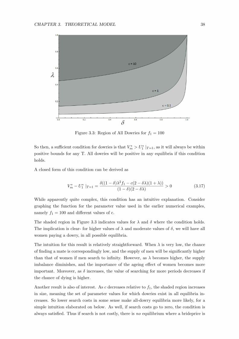
CHAPTER 3. THEORETICAL MODEL 38
Figure 3.3: Region of All Dowries for f1 = 100
So then, a sufficient condition for dowries is that V ∗m > U∗1 |T=1, as it will always be within
positive bounds for any T. All dowries will be positive in any equilibria if this condition
holds.
A closed form of this condition can be derived as
V ∗m − U∗1 |T=1 =δ((1− δ)λ2f1 − c(2− δλ)(1 + λ))
(1− δ)(2− δλ)> 0 (3.17)
While apparently quite complex, this condition has an intuitive explanation. Consider
graphing the function for the parameter value used in the earlier numerical examples,
namely f1 = 100 and different values of c.
The shaded region in Figure 3.3 indicates values for λ and δ where the condition holds.
The implication is clear- for higher values of λ and moderate values of δ, we will have all
women paying a dowry, in all possible equilibria.
The intuition for this result is relatively straightforward. When λ is very low, the chance
of finding a mate is correspondingly low, and the supply of men will be significantly higher
than that of women if men search to infinity. However, as λ becomes higher, the supply
imbalance diminishes, and the importance of the ageing effect of women becomes more
important. Moreover, as δ increases, the value of searching for more periods decreases if
the chance of dying is higher.
Another result is also of interest. As c decreases relative to f1, the shaded region increases
in size, meaning the set of parameter values for which dowries exist in all equilibria in-
creases. So lower search costs in some sense make all-dowry equilibria more likely, for a
simple intuition elaborated on below. As well, if search costs go to zero, the condition is
always satisfied. Thus if search is not costly, there is no equilibrium where a brideprice is

CHAPTER 3. THEORETICAL MODEL 39
paid between a woman and a man.
3.8 Comparative Statics
It also serves to ask how a change in c will change an established equilibria. The following
result is of prime importance.
Proposition 8. If women stay in the market for a finite number of periods T , a marginal
increase in search costs will cause all dowries to fall, in any equilibrium
Proof. Recall the Dowry function given in Equation (3.5). One can then see that-
δDt
δc= 1/2[
δV ∗mδc− δU∗t
δc]
Take the second argument first.
Beginning from the telescoped version of U1 outlined above, we can derive
U∗t =λ
2
T∑t=τ
θt−1(ft − δV ∗m)−T∑t=τ
θt−1c
where θ = (1− λ2 )δ.
Taking the derivative w.r.t c yields
δU∗tδc
= −λδ2
T∑t=τ
θt−1δV ∗mδc−
T∑t=τ
θt−1
Now consider V ∗m. Manipulating Equation (3.16), we can show
V ∗m =λm2
∑Tt=1 µt[ft − δU∗t+1]− c
1− θm
where θm = (1− λm2 )δ. Taking the partial derivative,
δV ∗mδc
= − 1
1− θm−
λmδ2
∑Tt=1 µt[
δU∗t+1
δc ]
1− θm
When T=1, solving these equations gives
δV ∗mδc− δU∗1
δc|T=1 =
−1
1− θm− λδ
2(
1
1− θm) + 1 < 0

CHAPTER 3. THEORETICAL MODEL 40
When T =∞ ,δU∗t
δc =δU∗t+1
δc =δU∗
1δc , as a woman entering the market in period t will expect
to search just as many times as a woman in period t+ 1.Thus we will have
δV ∗mδc
= − 1
1− θ−
λ2δU∗t
δc
1− θ
δU∗tδc
= − 1
1− θ−
λ2δV ∗mδc
1− θ
Of course, when T =∞ then θm = θ as λm = λw.
Solving these equations yields
δV ∗mδc− δU∗t
δc|T=∞ = 0
Lastly, δDtδc is monotonically increasing in T , and so must lie between these bounds.
To see this, first note thatδU∗t
δc < 0 ∀ T . This is because λδ2δV ∗mδc < 1 , even evaluated at
the maximal effect of 11−θm . This also establishes that
δU∗t
δc is monotonically decreasing in
T .
Now take δV ∗mδc . It is clear it is monotonically increasing in T . This follows from the fact
that − 11−θm is increasing in T , as λm always increases with T, −
λδ2
1−θm is decreasing for the
same reason, and as outlined above,δU∗t
δc is decreasing.
So the first term in δDtδc is increasing, minus a decreasing term, so all up δDt
δc must be
monotonically increasing in T .Thus it must always be within negative bounds.
The intuition behind this result is straightforward. If women must drop out in some period
T, then they spend less time on average searching for a mate. If this is the case, then
women can expect to pay the fixed fee c less times in the future, and thus a rise in the fee
will have proportionally less of an effect on their continuation value than it will on males’.
As dowries are negotiated through continuation values, they must then fall.
However, it is not quite as strong a result as one might hope. It can be seen that if the
rise in c is large enough, it can knock the market into another equilibrium. That is, a
sufficient rise in c will cause a woman of age T to drop out of the market. This will shrink
the supply of women, and the effect on dowries is ambiguous.

Chapter 4
Extension- Heterogeneity of Males
One obvious simplification of this search theory of dowries is that men are all identical,
whereas women are heterogeneous. As explained above, this was done to capture the
effect of a decaying worth of women over time. In real life, however, men are obviously
not identical, and the theory should attempt to capture this heterogeneity.
One way in which to do this is to allow the worth of men to decline with age as well,
but at a slower rate than women. However, in the infinite horizon case the model quickly
becomes intractable.
Instead, another way to proceed is to allow for different qualities of men, whose worth
is static through time. This is modelled by assuming that there are two types of men,
educated and uneducated 1.These qualities are exogenous and are determined in some away
outside the marriage market.
It is further assumed that an educated man has more to bring to a marriage (perhaps
through higher wages in the labour market, or more stimulating dinner conversation), and
thus his output when matched with any woman of age t is always more than that of an
uneducated man.
Consider the following model.
There are two types of men, Educated and Uneducated. Each period nature adds Xe
Educated men and Xn Uneducated men to the market, with Xe + Xn = X. Nature also
adds X women to the market each period.
If a woman marries an educated man, the surplus is Yt,e, and if she marries an uneducated
man, the surplus is Yt,n, with Yt,e > Yt,n.
Women age as follows: up to period T, a match with her will produce Y1,j , and then in
period T and onwards she will produce Y2,j , with Y1,j > Y2,j . Call a woman Young if
t < T , and Old if t ≥ T
This is a significant simplification on A.1, but is implemented for two reasons. Firstly,
the situation where old women drop out of the market and affect the overall supply of
1One could also use the distinction Wealthy and Poor, with little difference.
41

CHAPTER 4. EXTENSION- HETEROGENEITY OF MALES 42
women has been studied above, and the point of this extension is instead to study the
effect of introducing different types of males. Thus the simplest specification possible is
used. Secondly, it is believed that this form of the production function well captures the
underlying ageing dynamics. The reason is that though the drop is sudden at some date
T , women can see it coming, and as they approach this date, their continuation value
worsens, lowering their bargaining power.
So there are then four cases for the marriage surplus-
Y =
Y1,e if man is Educated an t < T
Y2,e if man is Educated and t ≥ T
Y1,n if man is Uneducated and t < T
Y2,n if man is Uneducated and t ≥ T
(4.1)
with Y1,e > Y2,e > Y1,n > Y2,n > 2c, which ensures a woman of any age will always pre-
fer to be married with an educated man. The surplus is split by Nash bargaining, as before.
The solution concept is virtually identical to that presented in the baseline case. Both
men and women will attempt to maximise utility in any period t by solving their problems
backwards- first choosing who to marry, and then whether to enter the search market.
They take the shadow prices V ∗E , V∗N and U∗t as given, as they are determined by aggregate
behaviour.
Now, the payoff of an Old woman who searches in period T must be given by
U∗T = max[pwT λw(ρ
2qTNq
NT (Y2,n − δV ∗N ) +
1− ρ2
qET (Y2,e − δV ∗E)) + (1− λw2
)δU∗, 0]
where ρ = XnX , or the chance that a woman will meet an Uneducated man, conditional on
meeting someone at all, and V ∗ (resp. U∗) is the constant continuation value for a man
(Old woman).
qEt is the probability that an Educated man will marry a woman of age t, the solution of
which is
qEt =
1 if
Yt,eδ − U
∗t+1 > V ∗E
0 ifYt,eδ − U
∗t+1 < V ∗E
∈ [0, 1] ifYt,eδ − U
∗t+1 = V ∗E
qNt and qtN are the probabilities that an Uneducated man will marry a woman of age t,
and the probability that a woman of age t will marry an Uneducated man respectively.
They follow identical logic to above. Note that it must be the case that qtE = 1.

CHAPTER 4. EXTENSION- HETEROGENEITY OF MALES 43
As before, the payoffs of all the Young women can be characterized as:
U∗T−1 = max[pwT−1λw(ρ
2qT−1N qNT−1(Y1,n−δV ∗N )+
1− ρ2
qET−1(Y1,e−δV ∗E))+(1−λw2
)δU∗T−c, 0]
...
U∗1 = max[pw1 λw(ρ
2q1Nq
N1 (Y1,n − δV ∗N ) +
1− ρ2
qE1 (Y1,e − δV ∗E)) + (1− λw2
)δU∗2 − c, 0]
Once again, we wish to know how the continuation V ∗E , V ∗N and < U∗t > emerge as a result
of the aggregate decisions over entering and matching decisions.
To do this, a mapping is constructed, which takes as its arguments (< pwt >, V∗N , V
∗E) and
maps it onto (< p′t >, V′N , V
′E , ) for all values of t ∈ 1, 2, ..., T.2
This mapping is defined as follows: Ψ(< pwt >, V∗N , V
∗E) = (< p′t >, V
′N , V
′E), where
p′t = argmax pwt λw(ρ
2qtNq
Nt (Yt,n − δV ∗N ) +
1− ρ2
qEt (Yt,e − δV ∗E)) + (1− λw2
)δU∗t+1 − c
The solution is thus:
p′t =
1 if λw(ρ2q
tNq
Nt (Yt,n − δV ∗N ) + 1−ρ
2 qEt (Yt,e − δV ∗E)) + (1− λw2 )δU∗t+1 > c
0 if λw(ρ2qtNq
Nt (Yt,n − δV ∗N ) + 1−ρ
2 qEt (Yt,e − δV ∗E)) + (1− λw2 )δU∗t+1 < c
∈ [0, 1] if λw(ρ2qtNq
Nt (Yt,n − δV ∗N ) + 1−ρ
2 qEt (Yt,e − δV ∗E)) + (1− λw2 )δU∗t+1 = c
V ′E is given by
V ′E = pmE λm2
(T−1∑t=1
µtqEt (Y1,e−δU∗t+1)+(1−
T−1∑t=1
µt)qET (Y2,e−δU∗))+(1−λm
2)δV ∗E−c (4.2)
where µt is the probability of meeting a Young woman of age t, given by((1−λ)δ)t−1pwt
W , and
(1−∑T−1
t=1 µt) is the probability of meeting an Old woman.
Analogously,
2It is only necessary to define the mapping up to T, because all Old women are identical. If one enters,they all enter, so to speak, and so though they may keep coming back to the market at any date after T,pT captures the relevant information for all of them.

CHAPTER 4. EXTENSION- HETEROGENEITY OF MALES 44
V ′N = pmNλm2
(T−1∑t=1
µtqNt q
tN (Y1,n−δUt+1)+(1−
T−1∑t=0
µt)qNT q
TN (Y2,n−δU∗))+(1−λm
2)δV ∗N−c
(4.3)
The first task is to establish the existence of an equilibrium in the marriage market.
Again, this equilibrium takes the form of a fixed point where V ∗N = V ′N , V∗E = V ′E , and
U∗ = U∗T = U∗T+i.
Proposition 9. There exists an equilibrium in the marriage market with heterogeneous
males. Moreover, under A.2, if λ−δλ(1−ρ)−δλY1,e > 2c and ρ < δ(1−λ), then there is a positive
search equilibrium
Proof.
Lemma 4.1. The mapping Ψ(.) is convex-valued and upperhemicontinuous for all t ∈ T ∗
Proof. See Appendix
Then, by the application of Kakutani’s fixed point theorem, there must exist a fixed point.
This is the equilibrium.
Above all, we are interested in a positive search equilibrium, where some agents engage in
search for partners. The following Lemma gives a sufficient condition for this.
Lemma 4.2. Under A.2, if
• λ−δλ(1−ρ)−δλY1,e > 2c and
• ρ < δ − λδ,
then at least some agents will enter the market
This Lemma is the multiple male type form of Lemma 3.7, explored under the specific
probability functions in A.2. The general sufficient condition is
λm(M,W |T = 1, V ∗N = 0)Y1,e > 2c
but in the interest of exposition and clarity, the closed form solution is explored.
Proof. All that is required for a positive search equilibrium is that some agents find it in
their interest to enter. A natural angle of attack is to examine the minimum conditions
necessary for the highest quality agents to enter.

CHAPTER 4. EXTENSION- HETEROGENEITY OF MALES 45
What do we need for the very youngest women, and the educated men, to enter and pair
up profitably? If women of age t=1 enter, then for a man to be able to bargain over
positive surplus requires
λmY1,e > 2c
Using our previous assumption on λm,
λm = λW
M
= λX
X((1−ρ)−δλ)1−δ
=λ− λδ
(1− ρ)− λδ
For this equation to hold true, there needs to be less women then men, or W < M , which
requires 1−δ(1−ρ)−λδ < 1. Alternatively, we need
ρ < δ(1− λ)
Obviously, if potential gain is positive from the men’s perspective (λmY1,e > 2c), then it
must also be from the women’s perspective (λY1,e > 2c). So if both women of age t = 1
and educated men meet, they can match with positive gain, and we will have a positive
search equilibrium.
From here it serves to examine the types of possible equilibrium that may emerge. As
stated above, in this section the case of most interest is where Old women enter with
probability 1, such that the only effect driving dowries is the ageing effect. One result is
immediately of interest.
Proposition 10. A fully separating equilibrium can never exist in this marriage market
Proof. There are two types of fully separating equilibrium which are conceptually possible
here. Consider the interesting one first, where Young women marry Educated men and
Old women marry Uneducated men, and all enter with probability one.
The continuation value for an Old woman would be constant if such an equilibrium existed,
and given by-
U∗ = λ(ρ(1/2(Y2,n − δV ∗N + δU∗))) + (1− λ)δU∗ − c
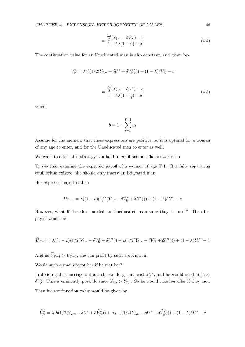
CHAPTER 4. EXTENSION- HETEROGENEITY OF MALES 46
=λρ2 (Y2,n − δV ∗N )− c1− δλ(1− ρ
2)− δ(4.4)
The continuation value for an Uneducated man is also constant, and given by-
V ∗N = λ(b(1/2(Y2,n − δU∗ + δV ∗N ))) + (1− λ)δV ∗N − c
=λb2 (Y2,n − δU∗)− c1− δλ(1− b
2)− δ(4.5)
where
b = 1−T−1∑t=1
µt
Assume for the moment that these expressions are positive, so it is optimal for a woman
of any age to enter, and for the Uneducated men to enter as well.
We want to ask if this strategy can hold in equilibrium. The answer is no.
To see this, examine the expected payoff of a woman of age T-1. If a fully separating
equilibrium existed, she should only marry an Educated man.
Her expected payoff is then
UT−1 = λ((1− ρ)(1/2(Y1,e − δV ∗E + δU∗))) + (1− λ)δU∗ − c
However, what if she also married an Uneducated man were they to meet? Then her
payoff would be-
UT−1 = λ((1− ρ)(1/2(Y1,e − δV ∗E + δU∗)) + ρ(1/2(Y1,n − δV ∗N + δU∗))) + (1− λ)δU∗ − c
And as UT−1 > UT−1, she can profit by such a deviation.
Would such a man accept her if he met her?
In dividing the marriage output, she would get at least δU∗, and he would need at least
δV ∗N . This is eminently possible since Y1,n > Y2,n. So he would take her offer if they met.
Then his continuation value would be given by
V ∗N = λ(b(1/2(Y2,n − δU∗ + δV ∗N )) + µT−1(1/2(Y1,n − δU∗ + δV ∗N ))) + (1− λ)δU∗ − c
CHAPTER 4. EXTENSION- HETEROGENEITY OF MALES 47
which is greater than V ∗N .
This establishes that there can never be an equilibrium where educated men marry only
young women, and uneducated men marry only old women. What about the converse
situation? This can also never be the case, for if an educated man and young woman met,
it is in both their interests to match and deviate from such a strategy, by the same logic
above.
Thus there can never be a fully separating equilibrium in this marriage market.
This is somewhat intriguing. Firstly, it contradicts the work of Becker (1991) on frictionless
marriage markets, a key result of which is that matching should be perfectly assortative
(higher quality men will match with higher quality women), and accords with Shimer and
Smith (2000). Because of the vagaries of the search market, a young woman must be
willing to broaden the set of men she finds acceptable.
However, while the model admits the possibility of a pooling equilibrium (conditions of
which are omitted here, but relatively easy to derive), from an intuitive standpoint we are
more interested in a least a partially assortative matching result- for this is precisely how
the romantic world works in practice. The model admits this possibility as well.
Define d1 = Y1,e − Y2,e and d2 = Y1,n − Y2,n
Proposition 11. If d1 and ρ are sufficiently large and d2 and c sufficiently small,a par-
tially separating equilibrium exists where:
• Old women will enter with probability 1
• Educated men will only marry young women, but all other actors will marry whomever
they meet.
Proof. This proof is analogous to the proof of Proposition 3, so in the interest of brevity
is only sketched.
If Old women enter with certainty, then λw = λm = λ.
For an Educated man not to marry an Old woman if he meets her, we must have
δV ∗E =δ λ2 (Y1,e − δ
∑T−1t=1 µtUt)− c
1− θ> Y2,e
This is clearly possible if d1 is large and c is small.
For an Uneducated man to agree to marry an Old woman, we must have
Y2,n > δhV ∗N (Y1,n, Y2,n)

CHAPTER 4. EXTENSION- HETEROGENEITY OF MALES 48
which will be possible if d2 is sufficiently small.
For a Young woman to agree to marry an Uneducated man, it must be that
Y1,n > δhU∗t (ρY1,n, (1− ρ)Y1,e)
This will be possible if ρ is sufficiently large, that is, if the number of educated men in the
market is low.
Other conditions we require are that U∗, V ∗N > 0 sot that both Old women and Uneducated
men enter the market with probability 1, which can also be solved out as functions of the
parameters. This rests on the fact that c is sufficiently small.
Again, as in Proposition 3, these serve as sufficient conditions as well.
Feeling that this equilibrium is very natural, its properties are now studied to examine
dowries.
Proposition 12. At this equilibrium-
i) if a woman of any age marries an educated man, she must pay a dowry.
ii) the average dowry of the system is positive
Proof. The proof of part i) follows similar logic to the proof of Proposition 7, and thus
appears in the Appendix.
The intuition is familiar- because λm = λw at this equilibrium, the ageing effect ensures
that when a woman matches with a high-quality man, she must pay a dowry. However,
this is not true for an Uneducated man. If such a man meets a very young woman, the
chance of meeting a higher-quality man next period is factored into her decision. If they
are to marry, it is possible he may have to transfer some utility to her to convince her to
settle.
As for part ii), one can think of the average dowry of the system as the dowry payments
of each woman of age t weighted by the size of her age cohort, conditional on meeting a
man of a certain education. Thus, denoting average dowry as ∆, we have
∆ =∞∑t=1
µtDj,t = δ/2∞∑t=1
µt[ρV∗N + (1− ρ)V ∗E − U∗t ]
=δ
2[ρV ∗N + (1− ρ)V ∗E −
∞∑t=1
µtU∗t ]
This expression must be positive. To see this, a woman’s expected payoff at age t at this
equilibrium is given by

CHAPTER 4. EXTENSION- HETEROGENEITY OF MALES 49
U∗t =λ
2[ρ(Yt,n − δV ∗N + δU∗t+1) + (1− ρ)(Yt,e − δV ∗E + δU∗t+1)] + (1− λ)δU∗t+1 − c
Rearranging U∗t+1 in the expression and multiplying both sides by∑∞
t=1 µt gives
∞∑t=1
µtU∗t =
λ
2
∞∑t=1
µt[ρ(Yt,n− δV ∗N − δU∗t+1) + (1− ρ)(Yt,e− δV ∗E − δU∗t+1)] + δ
∞∑t=1
µtU∗t+1− c
noting, of course, that∑∞
t=1 µtc = c, as the probabilities must sum to one.
However, as U∗t+1 ≤ Ut, with this holding with strict inequality ∀ t < T , we may write
(1− δ)∞∑t=1
µtU∗t <
λ
2
∞∑t=1
µt[ρ(Yt,n− δV ∗N − δU∗t+1) + (1− ρ)(Yt,e− δV ∗E − δU∗t+1)]− c (4.6)
Now Equations (4.2) and (4.3) can be rewritten as
(1− δ)V ∗E =λ
2(T∑t=1
µt(Yt,e − δU∗t+1 − δV ∗E))− c
(1− δ)V ∗N =λ
2(∞∑t=1
µt(Yt,n − δU∗t+1 − δV ∗N ))− c
It is the easy to verify that the R.H.S of (4.6) is less than
(1− δ)(ρV ∗N + (1− ρ)V ∗E). So, cancelling the common (1− δ) gives
∞∑t=0
µtU∗t < ρV ∗N + (1− ρ)V ∗E
Thus we have ∆ > 0.
This is an intriguing result. The logic of part i) of Proposition 12 should convince the
reader that there is no reason why a young woman may not receive a brideprice from an
uneducated man in equilibrium. However, part ii) assures us that even if this is the case,
the average dowry of the system will still be positive. The expectation of declining worth
for young women is enough to convince them to settle now with anyone, before it is too
late.
Observation 4.1. This result can also be shown to shown to hold in any equilibrium
(pooling or partially separating) where women enter at all ages, so that λw = λm.

CHAPTER 4. EXTENSION- HETEROGENEITY OF MALES 50
The obvious next step is to obtain a sufficient condition for dowries in any equilibrium as
was done in the baseline case. However, due to time constraints this was not possible.
4.1 Generalization to a Continuum of Male Worth
It is simple to extend this argument to n types of males, as all the same methods outlined
above can be used (with clearly exponential computational complexity). On reflection,
Propositions 9 - 12 will also hold in an n-type economy.
What is interesting is considering a continuum of male worth. This too should in principle
be possible. Consider indexing males on an atomless continuum of fitness [0, 1].
We will then have Ut given by
Ut =λw2
[
∫ 1
0g(i)(Yt,i − δV ∗i + δUt+1)di] + (1− λw)δUt+1 − c
where g(i) is the probability density function of male worth.
The problem arises from trying to apply the standard fixed point theorem to this problem,
to prove the general existence of an equilibrium. The author is not sure how this might
be done.
4.2 A Note on Multiple Searches per Period
A simplifying assumption of this thesis is that women and men may only search once per
period. One must ask, how realistic is this? A man or a woman in the real world will
search for years (or even decades) for the perfect partner. While we can make T arbitrarily
large to cover this situation, the question still arises, what would change if we incorporate
this possibility of multiple searches per period?
Here a preliminary answer will be given- functionally nothing.
Let us return to the baseline model, with homogeneous men, and define the output function
of marriage a little more generally. Permit agents to search z times in period t, but have
the output function f(m,wt) defined over t only.
A modeling problem immediately arises, in that now the matching probabilities are func-
tions of the time period in which one finds oneself, or more specifically the particular z.
This owes to the fact that if X agents are entering in period t, assuming some matches
in z1 there will be less agents in z2. So one then must make the simplifying but natural
assumption that instead of X agents of both sexes entering in period t, x agents of age 1
enter in each sub-period z, with x = Xz .
However, if one makes this assumption, the problem is formally identical to the model
derived above, with all the same results.

Chapter 5
Implications of Results
5.1 What Really Causes Dowries?
As has been outlined, most of the economic literature has assumed that dowries arise as a
price to clear an imbalanced marriage market. Indeed, much of the most recent work (e.g
Self and Grabowski (2009)) merely assumes the existence of a dowry system, and then
asks how various attributes of the bride and groom (caste, age, wealth) will change the
level.
This thesis has provided a new explanation for the source of dowries, based on differential
ageing in favour of men. The model presented is consistent with the standard model, while
extending its insights. Supply and demand of men and women may be important factors,
but ageing effects may be even more important, and go some way to explaining the poor
record of the standard model on a micro-empirical level.
5.2 Empirical Applications
This thesis throws up some eminently testable empirical applications, some of which are
confirmed by existing studies and others which will require new work.
The first relates to the age structure of dowries that this thesis has constructed. The
model predicts that older women will pay higher dowries than younger women, as a result
on having limited options and a declining value of search. This prediction is confirmed by
some studies, for example (Edlund, 2000), who found that dowries rise with a woman’s age.
There is also support that this ageing effect is not a uniquely South Asian phenomenon,
in that it occurred in other historical dowry paying societies, such as Renaissance Tuscany
(Botticini, 1999), which lends generality to the results. Specifically, Botticini reports that
each additional year in the bride’s age led to a statistically significant increase of 8 gold
florins in the dowry paid (around 6% of average dowry size).
The data also supports the corollary of A.1, that the worth of men does not similarly
decay with time. In fact, it has been well-documented empirically that average dowry size
51

CHAPTER 5. IMPLICATIONS OF RESULTS 52
in fact increases with groom age (Dalmia, 2004; Edlund, 2000), even controlling for wealth
which usually rises with age.
However, there is a problem with simply regressing dowry size on bridal age and using it to
justify this hypothesis. There remains the possibility that older women pay higher dowries
simply because men find them less attractive, and not because they are less productive in
the marriage. It would require some serious thought on how one separate the ageing effect
due to declining reproductive ability from any taste-based discrimination that occurs from
physical beauty. The issue, is of course, complicated by the simultaneous interaction of
both effects due to evolution- it is likely men find younger women more attractive precisely
because of the higher chances of conception.
In a perfect world, the empiricist would like to gather a dataset on dowries that also
contains an objective measure of the bride and groom’s physical appearance (perhaps based
on the aggregation of several subjective opinions). Such objective measures of beauty have
been used before in labour economics, most notably in the famous study by Hamermesh
and Biddle (1994) on the effect of physical beauty on labour market outcomes. One
might then be able to control for such simultaneous interaction with standard empirical
techniques, and separate out the hypothesized general age effect for women.
The second relates to the issue of search costs. This issue is (empirically speaking) virgin
land for economists. It would form interesting research in its own right to investigate the
hypothesis raised in this thesis, that dowries may increase with a decline in search costs.
Prima facie, this should be be testable.
How one would go about it is the unique joy of empirical work. One possible dimension
to explore is that of communication technology, and another is greater population density,
which enhances the possibility of random meetings between sexes. Both of these intu-
itively would imply that search costs should be lower in urban areas and dowries higher,
controlling for individual characteristics, which could well be verifiable.
5.3 Banning Dowries- Some Theoretical Insight
As explained above, it is theorised that dowries generate significant externalities which
fall on the families of both parties, and the wider society. Studying and specifying these
externalities is a task that has barely begun, and models such as this are necessary to
move forward. However, while we wait for a more generally specified model, some small
things of interest may be said.
Let us for now make the simplifying conjecture that the externalities generated by dowries
outweigh the benefits derived from the free exchange of two consenting adults, such that the
phenomenon is a negative one, on balance. Banning the practice is the logical conclusion.
Yet it is patently obvious that, in the case of India at least, the government is not capable
of fully banning the practice. Despite being illegal since 1961, the practice appears no less

CHAPTER 5. IMPLICATIONS OF RESULTS 53
prevalent than it was back then, and has perhaps spread to areas and castes where it was
not observed before (Anderson, 2007a). So a more realistic way of evaluating the policy
is the following.
Suppose the government imposes a heavy penalty on those families it catches which have
participated in dowry, but there is a non-certain probability that it will be able to catch
the,. One can easily imagine that this marginally raises the fixed fee c that a party must
pay to search. As Proposition 8 shows, this would have the effect of lowering the dowry
level in an established equilibrium, as well as decreasing the set of equilibria where all
women pay a dowry. Thus even an ineffective dowry ban may be doing some good.
5.4 Why Do Dowries Decline With Modernisation?
The results could also be used to shed a sliver of light on the holy grail of dowry economics.
It is a truly magnificent and robust empirical phenomenon that the practice of dowry
declines with industrialisation and a sustained rise in the standard of living (Self and
Grabowski, 2009), such that no country with a GDP per capita over $US PPP 10,000
observes dowry or brideprice1. Several explanations have been proposed (Becker, 1981;
Anderson, 2003), but none is undisputed in the economics literature.
This thesis makes one potential explanation less plausible. One defining characteristic of
modernisation is that search costs in the marriage market are likely to fall. Increasing
urbanisation means that people are clustered closer together, and highly developed com-
munications technology makes it easier for them to communicate. However, this thesis
has showed that the most likely effect of falling search costs is an increase in dowry.
However, perhaps the decline has something to do with a change in the production func-
tion. Specifically, suppose it is the case that as a country enters the modern world, labour
market opportunities increase for women. This will alter the production function of mar-
riage, as women may also choose to produce some market income. If this is the case, their
worth will depend less and less on their unique ability to bear children, and the ageing
effect may disappear.
1In Europe, the practice declined at much lower levels of per capita income, sometime in the 18thCentury.

Chapter 6
Conclusions
As with any research, this piece is not without weaknesses. Before concluding, it serves
to briefly mention them in order to contextualise the model and its usefulness.
A reader familiar with South Asian culture is likely to point to two observations which
this thesis abstracts from. The first is the importance of caste in marriage. In this search
model, caste is entirely absent, but this is not considered to be a serious defect. For
one, the interaction of caste and dowries has been well-studied in the literature by many
authors. Furthermore, the model is well able to bear the imposition of caste without
too much difficulty. One can consider caste as a quality or desirableness indicator, in
which case it can be modelled just as education was. A more interesting question arises if
marriage is difficult or impossible between castes, which will fragment the search market.
This too is unproblematic in the basic case (if castes cannot intermarry, each may be
studied in isolation). However, there is a possibility that marriages between different
castes are asymmetric based on sex. There exists convincing evidence that women in
India are encouraged to marry into a higher caste than their own, but severely penalised
for marrying into a lower caste (so-called hypergamy). This problem has been well studied
by Anderson (2000; 2003; 2007b), and the author does not believe that this model has any
value to add to the question.
The second observation revolves around the fact that dowries and marriages are often not
the result of decisions by the bride and groom, but by the families of both parties, who are
instrumental in the entire matching process. How does the search model account for this?
If one is willing to make a single simplifying assumption- that households will try and
maximise the utility of their children- the problem is a non-issue, and all the techniques
above will apply.
One assumption in the model is clearly unsatisfying, in the sense that it perhaps abstracts
too far from reality. This is the assumption on a fixed birth rate- that each period nature
adds X agents of age t = 1 to the market. A nice aspect of this assumption is that it allows
a steady state to emerge in equilibrium, which is perhaps why it was also used by Sautmann
(2009). However, it also means that the children born in a period are independent of the
matches that formed in the previous period, something that is at best unusual and at
54

CHAPTER 6. CONCLUSIONS 55
worst a flaw in the description of the marriage model. Matters are further complicated
if one considers that a higher level of dowries may induce female infanticide, and thus
affect the birth rate. Trying to formally account for more realistic birth dynamics proved
unfruitful, as as a steady state was unable to be obtained with the author’s abilities.
The other way that search models deal with this problem is to fix the population size
and allow for exogenous dissolution of matches in each period, so that some fraction of
searchers must return to the market in each period. In a labour market this means a
random separation decision (Mortensen and Pissarides, 1999), in a marriage market this
means divorce (Smith, 2006). However, considering the nature of the model and the huge
focus on ageing dynamics, the utility of this approach was limited; and old women who
divorces might have no prospect of returning to the market, meaning the market shrinks
over time and eventually collapses without births.
This thesis has critiqued the standard model of dowries for not accounting for search
frictions, and has showed that doing so can substantially change the conclusions of theory.
However, in emphasising the frictional nature of the process, it is possible one has gone
too far in abstracting from the role of competition. In this model, competition with agents
of the same sex only enters through the matching probability functions. This is somewhat
undesirable, for competition seems to be a central feature of romantic interaction.
In further research, it may be of some interest to construct a hybrid search model, which
still features some competition. That is to say, a search model without the feature of single
pair meetings in time t. How one may do this is an open question, for it would not be
a trivial exercise, and the author is not aware of any previous work done on the subject.
One potential way forward is to keep the notion of a market, but introduce an element of
randomness in the process of arrival at the market, such that once a decision to search has
been made, the probability of participating in the market is not unity. One may then use
the techniques developed in this model (asymmetric ageing and intertemporal bargaining)
to construct a complete statement of dowries.
The model presented herein is a small part of a well-established trend in economics to con-
sider all aspects of human interaction within its domain. Applying economic methodology
to questions of family life and emotional interaction has been very successful in the past.
It is the hope of this author that investigations such as this will continue to illuminate the
remarkable complexities of human relationship.

Appendix A
Appendix
Proof of Lemma 4.1
The logic of the proof is similar to Lemma 3.1.
Before beginning, consider the nature of the mapping more closely. Choosing any pair of
V ∗N and V ∗E will fully determine the vector of probabilities pwt , and then Equation (4.2)
will imply a linear relation for V ′E in V ∗E (or a family of linear relations) and V ′N in V ∗N
Now consider taking a sequence of V ∗N and V ∗E . As both increase, the value of U ′T must
decrease. We also know that the intercepts of V ′E and V ′N will be changing, due to the
change in the other part of the pair. This change is, of course, continuous- an ε change in
V ∗E will cause the intercept of V ′N to move by λmλwδ2ρ4 ε, and vice-versa.
We move along the continuous path in V ′E and V ′N until we reach the point where U ′Treaches zero. At this point, they will randomise, and there will be a family of linear
relations for both V ′N and V ′E , which include the possibility of p′T = 1 and p′T = 0. As
demonstrated earlier, at this point the correspondence is no longer continuous, but it is
still upperhemicontinuous. Moving past this point, the correspondence collapses again
into a single valued mapping for V ′E and V ′N , until we reach the point where U ′T−1 = 0 and
the process repeats.
This demonstrates the mapping is upperhemicontinuous. It is also convex valued, as any
point in V ′N and V ′N can be represented by a convex combination of another two points.
This derives from the fact that a linear relation is convex valued, and at the vertical line
points in the correspondence, all points can be represented by a convex combination.
This proves the lemma.
56

APPENDIX A. APPENDIX 57
Proof of Proposition 12, Part i)
If a woman of any age marries an educated man, she must pay a dowry.
Proof. We can write the payoffs of all women as
U∗1 =λ
2(ρ(Y1,N − δV ∗N + δU∗2 ) + (1− ρ)(Y1,E − δV ∗E + δU∗2 )) + (1− λ)δU∗2 − c
U∗2 =λ
2(ρ(Y1,N − δV ∗N + δU∗3 ) + (1− ρ)(Y1,E − δV ∗E + δU∗3 )) + (1− λ)δU∗3 − c
...
U∗T =λ
2(ρ(Y2,N − δV ∗N + δU∗T )) + (1− λ)δU∗T − c = U∗T+1 = U∗T+...
U∗1 then telescopes to
U∗1 =λ
2
T∑t=1
σt−1[ρ(Y1,N−δV ∗N+δU∗t+1)+(1−ρ)(Y1,E−δV ∗E+δU∗t+1)]+λ
2
σTρ(Y2,N − δV ∗N + δU∗T )
1− σ− c
1− σ
V ∗E and V ∗N can be written as
V ∗E =λ2 (∑T
t=0 µt(Y1,e − δU∗t+1 + δV ∗E))− c1− σ
V ∗N =λ2 (∑∞
t=0 µt(Yt,n − δU∗t+1 + δV ∗N ))− c1− σ
By revealed preference (Proposition 11) ,
V ∗E > V ∗E =λ2 (∑∞
t=0 µt(Yt,e − δU∗t+1 + δV ∗E))− c1− σ
and of course, V ∗E > V ∗N
Now define two new variables, such that
U †1 =λ
2
T∑t=1
σt−1[(ρY1,N + (1−ρ)Y1,E− δV †EN + δU †1 ] +λ
2
σTρ(Y2,N − δV †NE + δU †1)
1− σ− c
1− σ
V †EN =λ2
∑∞t=1 µt(ρYt,N + (1− ρ)Yt,E − δU †1 + δV †EN )− c
1− σ

APPENDIX A. APPENDIX 58
Using the definition of µt (as it sums to infinity), we can write,
V †EN =λ
2
∞∑t=1
σt−1(ρYt,N + (1− ρ)Yt,E − δU †1 + δV †EN )− c
1− σ
One can note that V ∗E > V †EN and U †1 > U1
First of all, if T = 2 (a woman becomes old almost immediately), taking the difference
V †EN − U†1 yields
V †EN − U†1 |T=2 =
λ(1− ρ)σY2,E2− σ(2 + δλ(1 + ρ))
which is unambiguously positive, given ρ < 1.
Secondly, if T =∞ (that is to say, a woman never ages), then]
V †EN − U†1 |T=∞ = 0
Lastly, the difference V †EN −U†1 is monotonically decreasing in T , so it must lie with these
bounds. To see this, note a one period increase in T will increase V †EN byλ2σ
T (ρY1,N + (1−ρ)Y1,E− (ρY2,N + (1−ρ)Y2,E)), which is positive given the specifications
on the production function of marriage. But U †1 will increase by even more, specificallyλ2σ
T (ρY1,N + (1 − ρ)Y1,E − ρY2,N ) So the difference V †EN − U †1 will decrease by a netλ2σ
T ((1− ρ)Y2,E)
This shows that for any finite T 6= 1, V †EN − U†1 > 0. Now as V ∗E > V †EN and U †1 > U1 at
any T, then we have V ∗E > U1 at any T .
As U1 > Ut, then V ∗E > Ut. Going from the dowry function in Equation (3.5), if a woman
of any age marries an educated man, she must pay a dowry.

Bibliography
Anderson, S. (2000): The Economics of Dowry Payments in Pakistan. Tilburg Univer-
sity.
(2003): “Why Dowry Payments Declined with Modernization in Europe but are
Rising in India,” Journal of Political Economy, 111(2), 269–310.
(2007a): “The Economics of Dowry and Brideprice,” The Journal of Economic
Perspectives, 21(4), 151–174.
(2007b): “Why the Marriage Squeeze Cannot Cause Dowry Inflation,” Journal
of Economic Theory, 137(1), 140–152.
Arunachalam, R., and T. Logan (2006): “On the Heterogeneity of Dowry Motives,”
NBER Working Paper.
(2008): “Is There Dowry Inflation in South Asia?,” NBER Working Paper.
Atakan, A. (2006): “Assortative Matching with Explicit Search Costs,” Econometrica,
74(3), 667–680.
Banerjee, A., and E. Duflo (2007): “The Economic Lives of the Poor,” The Journal
of Economic Perspectives, 21(1), 141.
Becker, G. (1981): A Treatise on the Family. Harvard University Press.
Bhat, P., and S. Halli (2001): “Demography of Brideprice and Dowry: Causes and
Consequences of the Indian Marriage Squeeze,” Population Studies, 53(2), 129–148.
Billig, M. (1992): “The Marriage Squeeze and the Rise of Groomprice in India’s Kerala
state.,” Journal of Comparative Family Studies.
Bloch, F., and V. Rao (2002): “Terror as a Bargaining Instrument: A Case Study of
Dowry Violence in Rural India,” The American Economic Review, 92(4), 1029–1043.
Bloch, F., and H. Ryder (2000): “Two-Sided Search, Marriages, and Matchmakers,”
International Economic Review, 41(1), 93–116.
Botticini, M. (1999): “A Loveless Economy? Intergenerational Altruism and the Mar-
riage Market in a Tuscan Town, 1415–1436,” The Journal of Economic History, 59(01),
104–121.
59

BIBLIOGRAPHY 60
Botticini, M., and A. Siow (2003): “Why Dowries?,” The American Economic Review,
93(4), 1385–1398.
Brien, M., L. Lillard, and S. Stern (2006): “Cohabitation, Marriage and Divorce in
a Model of Match Quality,” International Economic Review, 47(2), 451–494.
Brown, P. (2009): “Dowry and Intrahousehold Bargaining: Evidence from China,” Jour-
nal of Human Resources, 44(1), 25.
Caldwell, J., P. Reddy, and P. Caldwell (1982): “The Causes of Demographic
Change in Rural South India: A Micro Approach,” Population and Development Review,
8(4), 689–727.
Chade, H. (2001): “Two-Sided Search and Perfect Segregation with Fixed Search Costs,”
Mathematical Social Sciences, 42(1), 31–51.
Cherlin, A., and A. Chamratrithirong (1988): “Variations in Marriage Patterns in
Central Thailand,” Demography, 25(3), 337–353.
C.I.A (2011): “The World Factbook,” Central Intelligence Agency, www.cia.gov.
Cornelius, T. (2003): “A Search Model of Marriage and Divorce,” Review of Economic
Dynamics, 6(1), 135–155.
Dalmia, S. (2004): “A Hedonic Analysis of Marriage Transactions in India: estimating
determinants of dowries and demand for groom characteristics in marriage,” Research
in Economics, 58(3), 235–255.
Dalmia, S., and P. Lawrence (2005): “The Institution of Dowry in India: Why it
Continues to Prevail,” The Journal of Developing Areas, pp. 71–93.
Das Gupta, M., and P. Bhat (1997): “Fertility decline and increased manifestation of
sex bias in India,” Population Studies, 51(3), 307–315.
Edlund, L. (2000): “The Marriage Squeeze Interpretation of Dowry Inflation: A Com-
ment,” Journal of Political Economy, pp. 1327–1333.
Esteve-Volart, B. (2004): “Dowry in Rural Bangladesh: Participation as insurance
against divorce,” London School of Economics.
FAO (2011): “Women, Agriculture, and Food Security,” Food and Agriculture Organisa-
tion.
Gale, D., and L. Shapley (1962): “College Admissions and the Stability of Marriage,”
The American Mathematical Monthly, 69(1), 9–15.
Goody, J., and S. Tambiah (1973): Bridewealth and Dowry. Cambridge University
Press.
Hamermesh, D., and J. Biddle (1994): “Beauty and the Labor Market,” The American
Economic Review.

BIBLIOGRAPHY 61
Johansson, S., and O. Nygren (1991): “The Missing Girls of China: A New Demo-
graphic Account,” Population and Development Review, 17(1), 35–51.
Klasen, S., and C. Wink (2002): “A Turning Point in Gender Bias in Mortality? An
Update on the Number of Missing Women,” Population and Development Review, 28(2),
285–312.
Lahiri, S., and S. Self (2007): “Gender Bias in Education: the Role of Inter-household
Externality, Dowry and other Social Institutions,” Review of Development Economics,
11(4), 591–606.
Maitra, S. (2006): “Can Population Growth Cause Dowry Inflation? Theory and the
Indian Evidence,” NBER Working Papers.
Mortensen, D., and C. Pissarides (1999): “New Developments in Models of Search
in the Labor Market,” Handbook of Labor Economics, 3, 2567–2627.
Murdock, G. P. (1967): Ethnographic Atlas. Pittsburgh University Press.
Piette, C., J. De Mouzon, A. Bachelot, and A. Spira (1990): “In-Vitro Fertil-
ization: Influence of Women’s Age on Pregnancy Rates,” Human Reproduction, 5(1),
56.
Qian, N. (2008): “Missing Women and the Price of Tea in China: The Effect of Sex-
Specific Earnings on Sex Imbalance,” Quarterly Journal of Economics, 123(3), 1251–
1285.
Quayle, R. (1988): A History of Marriage Systems. Greenwood Press.
Queller, D., and T. Madden (1993): “Father of the Bride: Fathers, Daughters, and
Dowries in Late Medieval and Early Renaissance Venice,” Renaissance Quarterly, 46(4),
685–711.
Rajaraman, I. (1983): “Economics of bride-price and dowry,” Economic and Political
Weekly, pp. 275–279.
Rao, V. (1993a): “Dowry Inflation in Rural India: A Statistical Investigation,” Popula-
tion Studies, 47(2), 283–293.
(1993b): “The Rising Price of Husbands: A Hedonic Analysis of Dowry Increases
in Rural India,” The Journal of Political Economy, 101(4), 666–677.
(2000): “The Marriage Squeeze Interpretation of Dowry Inflation: Response,”
Journal of Political Economy, 108(6), 1334–1335.
Sautmann, A. (2009): “Partner Search and Demographics: The Marriage Squeeze in
India,” mimeo.
Self, S., and R. Grabowski (2009): “Modernization, Inter-caste Marriage, and Dowry:
An Analytical Perspective,” Journal of Asian Economics, 20(1), 69–76.
BIBLIOGRAPHY 62
Sen, A. (1990): “More Than 100 million Women are Missing,” New York Review of Books,
37(20), 61–66.
Shimer, R., and L. Smith (2000): “Assortative Matching and Search,” Econometrica,
68(2), 343–369.
Smith, L. (2006): “The Marriage Model with Search Frictions,” Journal of Political
Economy, 114(6), 1124–1146.
Srinivasan, S., and A. Bedi (2007): “Domestic Violence and Dowry: Evidence from a
South Indian village,” World Development, 35(5), 857–880.
Suen, W., W. Chan, and J. Zhang (2003): “Marital Transfer and Intra-Household Al-
location: A Nash-Bargaining Analysis,” Journal of Economic Behavior & Organization,
52(1), 133–146.
Van Willigen, J., and V. Channa (1991): “Law, Custom, and Crimes Against Women:
The Problem of Dowry Death in India,” Human Organisation, 50(4), 369–377.
Wood, J. (1989): “Fecundity and Natural Fertility in Humans.,” Oxford Review of Re-
productive Biology, 11, 61.
Zhang, J., and W. Chan (1999): “Dowry and Wife’s Welfare: A Theoretical and Em-
pirical Enalysis,” Journal of Political Economy, pp. 786–808.