a scheme of notation and nomenclature for aircraft...
TRANSCRIPT

R. & M. Na. 3562, Part 3
M I N I S T R Y OF T E C H N O L O G Y
A E R O N A U T I C A L RESEARCH COUNCIL
REPORTS AND MEMORANDA
A Scheme of Notation and Nomenclature for Aircraft Dynamics and Associated Aerodynamics
by H. R. HOPKIN
Aero. Dept., R.A.E, Farnborough
Part 3--Aircraft Dynamics
LONDON: HER MAJESTY'S STATIONERY OFFICE
1970
pmcE £1 13s 0d [£1-65] NEa"
m~
,J
b ~ N . 6
PREFACE
For many years the notation and nomenclature used in the UK for aircraft dynamics has consisted of a basic scheme introduced by Bryant and Gates (R. & M. 1801, 1937) together with various additions and amendments due to Neumark, Mitchell, and others. Modifications were not co-ordinated and resulted in a complex mixture having at least two serious drawbacks. First, further rational extensions would be extremely difficult to make and probably confusing. Secondly, some parts of the scheme appeared to possess a pattern which in fact they did not possess, and this hidden ambiguity sometimes led to mistakes.
The present Report is the third in a series offive separate parts ofR. & M. 3562 in which a unified system of notation and nomenclature is described. The system will present few difficulties to those familiar with the scheme of Bryant and Gates and its variants, and has the great advantage that it has a built-in potential for extension. At the same time, reliable patterns are incorporated and furthermore a great deal of freedom is available to an author who wishes in special cases to simplify the notation without ambiguity--for example, by omitting suffixes.
The new system is the outcome of many years of discussion at the Royal Aircraft Establishment, in co-operation with the National Physical Laboratory. It has been adopted by the Royal Aeronautical Society for its Data Items on Dynamics. Moreover, agreements reached by the International Organisation for Standardisation on terms and symbols used in flight dynamics have so far been completely consistent with the principles of the system.
The Aeronautical Research Council hopes that publication in the R. & M. Series 'will encourage the acceptance of the new notation and nomenclature and its use in the general field of aircraft dynamics by workers in research establishments and universities and in industry.

A Scheme of Notation and Nomenclature for Aircraft Dynamics and Associated Aerodynamics
by H. R. HOPKIN
Aero. Dept., R.A.E., Farnborough
Part 3--Aircraft Dynamics
Reports and Memoranda No. 3562 Part 3*
June, 1966
Summary. A scheme of notation and nomenclature applicable to the dynamics and associated aerodynamics of
both aeroplanes and missiles is proposed. The proposals are intended to supersede the attempts made, notably by Bryant and Gates, to revise and extend the existing standard reference in this field, namely R. & M. 1801.
Part 1 contains an extensive introduction describing the main objectives and summarising a consider- able amount of historical background. It also lists the symbols, references, and most of the tables for the whole report, and provides an index. All illustrations are appended to Part 1, and copies included in the remaining parts where required.
Parts 2, 3, and 4 deal with basic notation and nomenclature, aircraft dynamics, and associated aero- dynamic data respectively, and they can be read almost independently of Part 1. A great deal of reference information is included in the main text and in the twelve appendices which comprise Part 5.
Parts 2 to 5 do not contain separate lists of symbols, references or indexes.
LIST OF CONTENTS
Section. 10. Equations of Motion
10.1. General equations of motion for a rigid object of constant mass
10.2. Equations of motion expanded in terms of derivatives of forces and moments
10.2.1. General form of the equations
10.2.2. Linearized equations for small disturbances from a steady state flight condition
10.2.3. Linearized equations for small disturbances from straight symmetric equilibrium flight
10.3. Equations of motion expanded in terms of aerodynamic-coefficient derivatives
*Replaces R.A.E. Tech. Report 66 200, Part 3 (A.R.C. 28 971), and includes the corrections and amend- ments listed in R.A.E. 66 200A.

11. Normalised Equations of Motion
11.1. Basis of normalising procedure
11.2. The dynamic-normalised equations
11.3. The aero-normalised equations
12. Stability and Response Quantities
12.1. Longitudinal stability and response
12.2. Lateral stability and response
13. Some Characteristics of Linear Dynamic Systems
13.1. General nomenclature
13.2. Measures of damping and frequency
13.3. A discussion of the merits of various measures of damping
14. Centres of Force and their Relation to Control Discriminants
14.1. Centres of pressure and aerodynamic centres
14.2. Control discriminants
14.2.1. Control discriminants for an aircraft in straight unbanked level flight
14.2.2. General interpretation of control discriminants
Acknowledgements
Illustrations--Figs. 6 to 11.
Detachable Abstract Cards
10. Equations of Motion. It is not practicable to set out equations of motion that are in a convenient form for all investigations
in aircraft dynamics. A large display of the application of the notation and nomenclature is provided by considering the equations relevant for a rigid object of constant mass in still air, and the following sections in this part of the report are entirely restricted to this case. However, the procedures to be adopted in more general cases are indicated in Appendices C and M. The equation~ of motion are presented here in their full component form, but a matrix form is given in Appendix M.
10.1. General Equations of Motion for a Rigid Object of Constant Mass. It will be assumed that there are no forces or moments present due to contact with the earth, but if
this were not true the symbols X, Y, Z, ~ , Jg, X would merely be replaced by X + X c, etc. according to the notation explained in Section 3. X, etc. represent the forces and moments other than gravitational and earth contact effects.

Section 10.1
The equations of motion of a rigid object of constant mass (m) in still air and referred to any system of body axes with origin at the c.g. are as follows :
m(ti + q w - rv) = X + mgx
J m(f~+ r u - p w ) = Y + m g y
m(Vv + p v - qu) = Z + mgz
Ix~ - Iy~(q 2 - r 2) - Izx(/" + pq) - Ixy((t - rp) - (Iy - I . ) qr = 5Y
I j t - Izx(r 2 - p2) _ ixr( : ) + qr) - Iy~(: ' - pq)---(I~ - Ix) rp = J g
I ~ - Ixy(p 2 - q2) _ Ir~( 4 + rp) - I~x(f~- qr) - (I x - I t ) pq = J f f
(10.1)
t (10.2)
The moments of inertia (Ix, Iv, I,) and the products of inertia (Irz, Izx, lxy) of a rigid object are of course constant. The symbols u, v, w; p, q, r denote the components of linear velocity of the c.g. and the angular velocity of the body respectively. The components of the weight are denoted by max, moy, mgz, and these may be expressed in various forms in terms of attitude angles, as shown in equations (5.14). A 'dot' over a variable denotes differentiation with respect to time.
It is usually convenient to reduce equations (10.1) and (10.2) to a concise form by dividing the force equations through by the mass, and each moment equation by the appropriate moment of inertia. We obtain
X f i + q w - r v - g x = - - ,
m
Y + r u - p w - Oy = - - , (10.3)
m
Z f f + p v - q u - g , = - - ,
m
5 : [~ + dx( q 2 - r 2) -t- ex(~ + pq) + f x( q - rp ) + bxqr = 7 - ,
i x
~1 + ey(r 2 - p2) +fy~ + qr) + dy(~- pq) + byrp = ~ ,
X + f~(p2 _ q2) + d~(~l + rp) + e.(p - qr) + bzpq = __I-- '
where dx, d r, d,; ex, e r, e, ;fx,fy,f,; bx, by, b, are the constant-of-inertia ratios defined in Section 9.
(10.4)
10.2. Equat ions o f M o t i o n E x p a n d e d in Terms o f Force and M o m e n t Derivatives.
10.2.1. General f o r m o f the equations. It is often convenient to expand the forces X, Y, Z and the moments £¢, ~ , j l : on the fight-hand sides of equations (10.1) and (10.2) in terms of the variables defining the motion, including the motivator deflections. There are several ways of doing this, since alternative sets of variables exist and also alternative expressions for the forces and moments. The notation required for coping with the various expansions is discussed in Part 4, and in this Section just one form of expansion is given for illustration.

Section 10.2.1
It should be noted that the equations of motion are very often put in a normalised form to suit the dynamic analysis, and that the force and moment derivatives are almost invariably normalised to suit the aerodynamicist. It is thought better, however, to postpone the presentation of normalised systems until Section 11, and to develop the equations first in their basic form.
We may express the force Z as a Taylor series in terms of increments* such as u', w', q', h', q ' , . . , from datum values Ue, We, qe, he, tie, and in terms of partial derivatives such as Z u = OZ/au, which are evaluated at the datum values Ue, We . . . . . The full Taylor expansion is written
T2 T s ) Z = Z e + T + ~ T + - - ~ ! + . . . Z , (10.5)
where T stands for the differential operator
T = h , ~ _ h + ( U , S ~ + v , ~ _ ~ + w , o _ ~ ) + { , a , ~ , c?'~ I" , O , ~ , O \ . . . .
Retaining only a few typical variables we thus write
Z = Z e + Z u u ' + Z w w ' + Z ~ v f v ' + Z q q ' + Z h h ' + Z . ~ r f + ½ Z u u u ' Z + . . . ,
and likewise
~/~ = J ~ e "1- M,,U' + Mww' + . . . .
the script letters not being required for the derivatives OJJ//Ou, etc. The reference values Z e , / J [ e are the values of Z, J / w h e n the expansion variables u, w . . . . have their datum values.
These partial derivatives Z . . . . . are called f o rce or moment derivatives, and it is convenient to define related concise derivatives, such as
X u Z w X u ~ - - - - ~ Zw - -
m m
Mq N~ mq - Iy n~ Iz
and likewise other concise quanti t ies such as z e = - Z e / m , so that on substituting in the equations of motion we obtain the compact forms
f i + q w - r v - g x + x e + x , u ' + x w w ' + . . . . . . = 0, etc.
*Sometimes variables representing deviations from the datum condition will be used which are functions of the increments and more convenient than the increments themselves. This is especially so for represent- ing perturbations in the attitude or position of the aircraft. Terms of this character are not included here since in free stream the aerodynamic forces and moments do not depend on attitude or position (other than altitude). A fuller discussion of the Taylor expansions will be found in Section 17, and the introduction of additional terms when required, for example on account of ground effect, is straightforward.

Section 10.2.1
The definitions of all concise quantities incorporate negative signs in order to make the majority of these quantities positive. When a concise quantity turns out to be negative it may be convenient to introduce a dressing to denote sign reversal, and the notation suggested is, for example,
NO FIv = - - n v = T z ,
so that ~v and N~, have the same sign. Such a 'reversed' concise quantity* could be referred to as 'n-v-neg'. As an example of the equations of motion we give below those obtained when the x and z-axes lie in
a plane of mass symmetry so that Iy z and l.y, and hence d~, dr, d~,f.,fr,f~, are zero.
fi + q w - rv - Ox + xe + XuU' + xww' + xqq' + x j v ' + Xhh' + x.~l' + . . . . 0
f; + ru - -pw -- 9y + Ye + yvV' + ypp' + yrr' + y¢~' + yc~' + . . . . _ . . . . . . . . 0
w + pv -- qu -- gz + ze + zuu' + zww' + zqq' + z j r ' + Zhh' + z~q' + . . . . 0
[~+ex(i '+pq)+bxqr +le+Ivv ' +lpp' +Irr' + l¢¢' + I f ' + . . . . . . . . . . . 0
+ ey(r 2 _ p2) + b 7 p + me + muU' + mww' + mqq' + mw~' + . . . . . . . . . 0
: + e~(~ - qr) + b~pq + n~ + nov' + npp' + n : ' + n¢~' + n f ' + . . . . . . . . 0
(10.6)
For principal axes the d's, e's, a n d f ' s would be zero. We have retained only a representative selection of the variables and of first-order derivatives. In general other terms, including higher-order derivatives, should be added as required, on the basis of (10.5).
This form of expansion is well suited to problems in which the motion can be treated as a disturbance from some fixed datum condition of flight: that is, the undisturbed flight is a steady condition correspond- ing to constant values of all variables except those that are naturally absent or redundant. The possible sorts of such undisturbed flight are
(a) level flight (straight or turning) at constant speed,
(b) non-level flight (straight or turning) at constant speed provided that the atmosphere can be treated as uniform.
In these steady states u, v, w, p, q, r, qb, ® are constant, while x, y, z, h, or W may be absent or redundant. It should be noted that if the motivators are fixed steady turning flight is possible about a vertical axis
only, and the datum values of the angular velocity components are related to the datum attitude as follows :
Pe = - f~e sin ®~,
qe = ~"~e sin Ce cos Oe,
ge = ~'~e COS (I) e COS •e,
where ~"~e = ~ f and denotes ihe steady resultant angular velocity.
It may be practicable to employ the form of expansion given above even when the datum values of some variables are not constant, provided that these values are defined in some functional way and always
*Confusion with mean derivatives (see Section K.2) is unlikely, but in emergency n-v-neg could be written as n ° or n~-.
Section 10.2.1
provided that increments relative to datum values are sufficiently small for the expansions to be valid. This technique will introduce derivatives that are functions of time or of other variables. As mentioned previously the suffixfshould replace e when datum values are not constant.
In some applications, for example stability investigations, the disturbances are assumed to be so small that the equations may be linearized, and the higher-order derivatives are taken as zero. Acceleration terms such as 0i + qw- r r ) are then written as (ti'+ qew'-r , ,v '+ w~q'-Ver'), and so on (see Section 10.2.2).
The more general types of undisturbed flight conditions such as climbing or diving in a non-uniform atmosphere, or flight at varying speed, are probably best treated by expanding the equations in terms of force- and moment-coefficient derivatives as set out in Section 10.3 ; otherwise the accumulating deviations in altitude or speed would entail a large number of terms in the Taylor series to preserve much degree of accuracy, and it would be difficult and rather artificial to relate the corresponding high-order derivatives to the aerodynamic data by relations like those in Appendix E.
To solve equation (10.6) we must use the kinematic relationships between the angular velocity com- ponents p, q, r and the rates of change of attitude angles, examples of which are equations (5.3) and (5.12). Normally the same attitude angles will be chosen for this purpose and for expressing the gravity components #x, q;, 9: as for example in equations (5.14).
We must also know how the increments in equivalent motivator deflections ~', ~l', (.', v', <~', I," vary. They may, for example, be fixed, or changed by an automatic pilot. In the latter case {', etc. may be functions not only of the increments in velocity components u', v', w', p', q', r', but also of perturbations in attitude angles: on occasion they may also depend on variables defining the deviations of the aircraft from some datum flight path. When such additional variables are introduced, further kinematic relation- ships will be required of the form given in Section 7.
In general, equations (10.6) would only be solved by means of a computing machine, but in particular cases the equations can be linearized and useful analytical solutions can result. Sections 10.2.2 and 10.2.3 give examples of a linearized treatment which may be applicable to all types of aircraft, including missiles, and an example especially pertinent to spinning missiles is given in Appendix F. Appendix G provides an example of the linearized equations expressed in terms of 'displacement' variables. Section 12 develops some aspects of the solution for the example of Section 10.2.2.
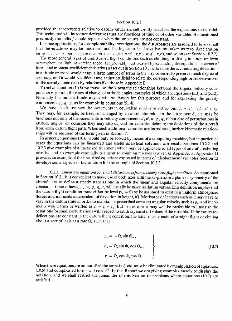
10.2.2. Linearized equations for small disturbances from a steady state flight condition. As mentioned in Section 10.2.1 it is convenient to make use of body axes with the xz-plane in a plane of symmetry of the aircraft. Let us define a steady state as one in which the linear and angular velocity components are constant--these values ue, re, We, Pc, qe, re will usually be taken as datum values. This definition implies that the datum flight condition must either be level (?e = 0) or be assumed to exist in a uniform atmosphere (forces and moments independent of deviation in height, h'). Motivator deflections such as ~ may have to vary in the datum state in order to maintain a prescribed constant angular velocity such as Pe, and incre- ments would then be written as 4' = ~ - is, but in this case it may well be preferable to linearize the equations for small perturbations with respect to arbitrary constant values of the variables. If the motivator deflections are constant in the datum flight condition, the latter must consist of straight flight or circling about a vertical axis at a rate f~e such that
Pe -~" - -{)e s i n Oe,
qe = ~e sin Oe COS ®e,
r r = ~ e COS (I) e COS (~e •
(10.7)
When these equations are not satisfied the terms in 4, etc. must be eliminated by manipulation of equations (10.6) and complicated forms will result 3z. In this Report we are giving examples merely to display the notation, and we shall restrict the remainder of this Section to problems where equations (10.7) are satisfied.

Section 10.2.2
With the choice of axes and datum condition specified above, the linearized~forms of equations (10.6) are as follows*.
fi' + qew' + w~q' - rev' - v~r' - 0'~ + Y, xuu' = 0
° t ! I r t ¢ I v + reu + uer - pew - w~p - 9y + Zyov = 0
° ! ¢ ! t t ! I
W q- pe p q- Vep -- qe u -- Ueq -- 9z -{- ~ Z w W = 0
[Y + ex( F + Peq' + qep') + bx(q~r' + req') + Y, lpp' = 0
q' + 2ey(rer' - PEP') + br(reP' + Pe r') + Y.mqq' = 0
~' + ez(ff - q~r' - req') + b~(p~q' + qeP') + Enrr' = 0
(10.8)
If in addition the angular velocity of the body is zero in the datum condition, considerable simplification ensues because Pe = qe = re = 0, and the equations become
a' + w e q ' - v e r ' - g'~ + Exuu' = 0,
(~' + Uer'-- W e f t -- g'y + ~,yvV' = 0,
if ' + v e P ' - Ueq' -- O'z + Zzww' -- O,
f)' + exO' + Zlpp' = O,
( t '+2mqq ' = 0 ,
~' + edY + Znrr' = 0.
(10.9)
It is often permissible to break up these equations into two groups of three : the first, third, and fifth constitute the longitudinal group, and the others the lateral group. It may then be possible to solve separately for the longitudinal variables u', w', q', 0 (and perhaps h'), and likewise for the lateral variables v', p', r', t~, ¢; and perhaps for variables defining the position of the aircraft c.g. relative to the datum flight path. When this is so, independent longitudinal and lateral motions can exist with no coupling between them.
The conditions for separating out the longitudinal equations are more stringent than those for the lateral equations, and the latter may therefore sometimes be immediately soluble when the longitudinal are not. It is then possible to substitute the solutions for the lateral variables into the longitudinal equations thereby making the coupling terms known functions and rendering these equations consequently soluble as a group.
The lateral equations of (10.9) can be treated separately if the cross derivatives such as Y, , Lw, N q a r e
zero, with the additional requirement that either (I) e and q~e must be zero or the longitudinal perturbations u', w', q', 0 must be zero if Vo or vE enter into the calculation.
The longitudinal equations can always be considered separately if the lateral perturbations v', p', r', c~, qJ are zero. When, however, lateral perturbations are permitted, we can separate the longitudinal equations of (10.9) only if the datum condition is symmetric (re and ~e zero) and if cross derivatives such as X v, Zp, Mr are zero, with the additional requirement that "z'~ must be zero if Uo, Wo, or wE enter into the calcul- ation.
*In practice no confusion is likely if the dashes are omitted when linearized equations are being used exclusively after they are established.
7

Section 10.2.3
10.2.3. Linearized equations for small disturbances from straight symmetric equilibrium flight. If the steady state is one of straight symmetric flight then the equations of motion are separable into longitudinal and lateral groups as explained in Section 10.2.2, since c,. = p,. = q,. = r,. = @~ = q',, = 0. From equations (10.9) and (5.15) the longitudinal equations are
l't' q'-glO+ XuU ' ' ] ' + XwW + (Xq + We) q . . . . . + x+w + x, v + x.r 1 + x~r¢ = O,
t t ! , l ¢ ")" t 7 i g" +geO+z.u +ZwW +(Zq--Ue) q +Z,i,W +z,v + . . r / q - . f l ( = O ,
(t' + m.u' + mww' + mqq' + m~,~' + m~v' + m.rf + m~x' = O,
(10.10)
and the lateral equations are
b'--g~c~--g2~ + y~v' +(yp--w~) p' +(y~+ u~)r' + y¢~' + y~5' + y~(' = O,
l p ' + e . f + l , . v ' + l , p ' + l / + l ¢ ~ ' + l , ~ 5 ' + l f ' = O,
i" + e~p' + n~v' + %p' + n J +n¢¢' + n~5' + n;(' = O .
(10.11)
It will be observed that in equations (10.10) and (10.11) the only 'dot ' derivatives included are those with respect to w, as is usual, but more could be included if they were found to be significant. Derivatives with respect to all six equivalent motivator deflections ~, t/, (, v, 5, x have been included for generality.
Letting D denote d/dt and rearranging the above equations, we obtain
(D-l-.xu) u' +(x~i,D+ xw)W' +(xq-t-we)q'-l-glO+ XvV'-k xn~' W x,~K' = O,
J z,,u' + [( l + z+) O + z,,,] w' + (Zq-U,.) q' + gzO + Z,V' + z,rf + z~c' = O,
m.u' + (mwD + mw) w' + (D + mq) q' + m~v' + m~tf + m~x' = O,
(10.12)
and
(D+ yv) v' + ( y p - w e ) p ' - .q lgp+(y ,+ue)r ' -g2~b + y¢~' + y~5' + y~ ' = O,
l,,v' +(D+Ip) p' +(exD+ lr)r' + l ~ ' +l~6' +l:( ' = 0,
nvv' + (ezD + np) p' + ( D + n,) r' + n¢~' + n~f' + n f ' = O .
(10.13)
The linearized kinematic equations required for solving the equations of motion are given in Sections 5.5 and 7, but are noted here for convenience:
DO = q' 1 !
Dz~ = w~. = - u' sin t~ e -J- W' COS 0~ e - - VeO t
J Dh' = - Dz~ = - w + = u' sin ®e-- W' COS ®e + VeO COS y~
(10.14)

Section 10,2.3
Dq~ = p'
D~ = r'
Dye, = v~, = v ' - V~q~ sin e~ + V~O cos ee
= V'--We~9-I.-Ue~I
(10.15)
The equations for v~ and w~ are needed when the motivator deflections depend on the distances y~ and z~ of the centre of gravity of the aircraft to the right of and below its datum flight path respectively, as for example when an automatic pilot controls the distances from an airport approach beam. The equations for 4;, 0, ~ are always required. The equation for h' is required for disturbances from level flight in a non- uniform atmosphere, or when the motivator deflections depend on h'--which may arise in level flight (Ye = 0), or in climbing or diving flight in an atmosphere that can be treated as uniform. For the non- uniform atmosphere cases, altitude-dependent t e rms Xhh', Zhh'. I'~lhh' must be added in equations (10.12).
The above equations may be modified so as to contain terms in ~1)'. O', W' instead of ~, O, ~. From equations (5.14) we have for ( I ) e = 0
g'~ = - g l O = - g t O ' ,
9'y = 01@+024 ' = 0 1 0 ' ,
g'z = --920 = - -g2 O ' ,
and to make these substitutions is the only modification required in equations (10.12) and (10.13), and also in (10.14), but (10.15) must be replaced by
D@' = p' + r' tan Oe, ]
DW' = r' sec (~)e,
Dy~ = v' - Ve~' sin e~ + VeW cos ?e.
(10.16)
10.3. Equations of Motion Expanded in Terms of Aerodynamic-Coefficient Derivatives. As explained in Section 10.2, expansions of the forces and moments in the form
Z = Z e + Z . u ' + . . .
are not suitable when the undisturbed flight involves varying conditions such as climbing or diving in a non-uniform atmosphere, or flight at substantially varying speed. Alternative expansions may be used, however, of the form
Z = 1 p V2S Cz
F /" T 2 T 3 ] (10.17)
where T is a differential operator given by
Pr ~P~ + q' ~qr + r' -~r~ ) ( . , 0 ., t? ., - + + . . . .
9

fi + qw - rv-Ox
Cz is a non-dimensional coefficient, p denotes the air density, S a representative area, and the normalised variables ~, f , pr, q~, rr, ~, &r,/~r,... are non-dimensional parameters corresponding to w, v, p, q, r, fi, ~, 6 . . . . respectively. Thus ~ represents an incidence angle, and qr is equal to ql/V, where I is the representa- tive length introduced when forming the moment coefficients, such as Cm = ~[/½ pV2SI. Further details are given in Part 4, but it is worth noting here that different values of I may be used for longitudinal and lateral moment coefficients, and that if we have Ct = ~/½pV2SI2, Cm =Jg/½pV2Sla, then the normalised variables should be correspondingly defined: pr = pl2/V, q~ = ql~/V.
If we write Cz, for OCz/Oa, and Cz~ for OCz/Oqr, etc., equation (10.17) may be written
z = ½ pV2S(Cz~+ Cz,~'+ Cz#f'+ Czqq'~+ .. .) ,
in which ½ pV2S may be replaced by ½ pM27S, where P denotes the air pressure, 7 the ratio of specific heats, and M the Mach number.
The reference value Cz~ and the derivatives Cz, . . . . are evaluated at the datum values of the parameters • , fl, pr . . . . . There is no objection to writing Cz, instead of Cz~, except for the possibility of confusion with the American Cz~, which does not have exactly the same meaning and is more analogous to our 2~. Similar remarks apply to all the coefficient derivatives.
We give below a typical set of equations in terms of expansions of the form (10. i7), and corresponding to equations (10.6 ~. As before we retain only a selection of variables and first-order derivatives.
6 + r u - p w - g r
½pV2SICxeq-Cx~'-k-Cx# fl +Cxppr+Cxqq~+Cxaar+Cxnrl + . . . ] _ v I v ~.l v
m
~v+ pv-qu-9~
= m re + Cr~a' + Craft + Crppr + Cv~rr + CreW' + Crf ' + ...
(lO.18)
= ½ pV2SICze+Cz~°~'m +Cz#f' +CzpP'~ +Czqq'r +Czar' r +Cznrf+.. "1
P + e~(f" + Pq) + bxqr - ½ pV2Sl2 I 1 l~--f--- Cle "~- Cl~t "~- Clflft + ClpP'e + Clrr'~ A" Cl~ ~' d- Cliff' -}- ...
q + er(r2 -p2) + brrp= ½ p V z Sl l I Cme + Cm~°g + Cm#fl' + Cmqq'r + Cma&'r d-Cmnq' "'" 1
~+ez(p-qr)+bzpq=½pVZSlz[ ' ' ' 1 iz Cne + C,,a + C,#fl' + C,ppr + C,,r~ + C,¢~' + C,f ' + ...
Section 10.3
10
Section 10.3
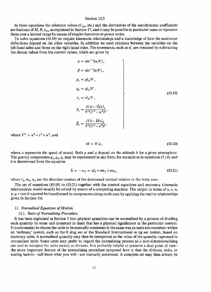
In these equations the reference values (Cxe, etc.) and the derivatives of the aerodynamic coefficients are funtions of M, R, Zoo, as explained in Section 17, and it may be possible in particular cases to represent them over a limited range by means of simpler functions or power series.
To solve equations (10.18) we require kinematic relationships and a knowledge of how the motivator deflections depend on the other variables. In addition we need relations between the variables on the left-hand sides and those on the right-hand sides. The increments, such as ct', are obtained by subtracting the datum values from the current values, which are given by
a = sin- 1(w/V), ]
/ fl = sin- 1(v/V),
p~ = pl2/V ,
q~ = qlz/V,
r~ = tiE~V, [
J
(Vf f - few) 11 &y = V2(V2_w2)4 $,
(Vf)- l?v) 12 1~ = Vz(VZ_v2) , ,
(10.19)
where V 2 = u 2 + v 2 + w 2, and
M = V/a, (10.20)
where a represents the speed of sound. Both p and a depend on the altitude h for a given atmosphere. The gravity components g~, gy, g~ may be represented in any form, for example as in equations (5.14), and h is determined from the equation
= - - W 0 = u / 3 - t - l ) m 3 + w n 3 , (lO.21)
where/3, ma, na are the direction cosines of the downward vertical relative to the body axes.
The set of equations (10.18) to (10.21) together with the control equations and necessary kinematic relationships would usually be solved by means of a computing machine. The output in terms of u, v, w, p, q, r can if required be transformed to components along earth axes by applying the matrix relationships given in Section 5.6.
11. Normalised Equations of Motion. 11.1. Basis of Normalisin# Procedure.
It has been explained in Section 2 that physical quantities can be normalised by a process of dividing each quantity by some unit (constant in time) that has a physical significance in the particular context. It is convenient to choose the units to be mutually consistent in the same way as units are consistent within an 'ordinary' system, such as the ft slug see or the Standard International m kg sec system, based on statutory units. A normalised quantity may then be interpreted as the value of the quantity expressed in normalised units. Some users may prefer to regard the normalising process as a non-dimensionalising one and to interpret the units merely as divisors. It is probably helpful to preserve a dual point of view: the more important feature of the normalising procedure proposed here is that the divisors, units, or scaling factors--call them what you will--are mutually consistent. A complete set may then always be
11

Section 11.1
derived by dimensional analysis once any three independent ones have been specified. In general, a non-dimensionalising or normalising process does not have this restriction on the divisors (which may even vary with time), and the system of units viewpoint may therefore help to emphasise the restriction when it applies. Another advantage of this interpretation is that only one symbol need be employed for denoting a physical quantity, although distinguishing marks may be required when, as in this Report, a quantity is expressed in more than one system.
It does not seem practicable to have one set of normalising units that will satisfy the needs of people who are chiefly interested in aircraft dynamics as well as people who are primarily interested in aero- dynamic forces alone. This Report suggests the adoption of two systems to meet the conflicting requirements. One is called the dynamic-normalised system and the other the aero-normalised system. Dynamical investigations will most often make use of equations of motion that have been normalised according to the dynamic system. The coefficients of the various terms of aerodynamic origin, however, will depend on aerodynamic data that are best normalised according to the aero-system. At this stage we postpone the detailed development of the aero-system until Part 4 and merely note that any quantity Z expressed in the aero-system may be denoted by ~ (Z 'dip'), and that 2 (Z 'cap') may be used to denote the same quantity expressed in the dynamic system. If the need should arise for emphasising that Z is being expressed in ordinary units, the symbol ~ (Z 'ord') could be used.
The normalised forms for presenting the equations and related aerodynamic data are essentially devised to deal with small disturbances from a datum condition, and corresponding units in the two systems are chosen to be simply related, or where possible identical. To this end a speed, such as u, is normalised by dividing its value by a unit of speed equal in magnitude to Ve, where Ve represents a datum value of the aircraft speed (V). We may thus write R = fi = u/Ve. Both u and Ve are usually expressed in ordinary units (o.u.), and the normalised value of u is the same whatever system of ordinary units is employed--as would be expected from a process which can be regarded as non-dimensionalising.
Similarly, the unit of force is made equal to 1 2 peVeS (o.u.), where Pe is a datum value of p, and the normalised forces may thus be directly connected with the non-dimensional force coefficients, such as Cz, which are formed by means of a divisor ½ pV2S. There are consequent connections, often fairly simple, between normalised derivatives of forces and moments and the derivatives of the corresponding force and moment coefficients (see Section 19).
The natural choice for datum values would be within the range of variation, and if the latter were small then the simple connections just mentioned would be realised. If, however, the range of variation were large there would be no advantage in this type of normalisation.
To complete the dynamic-normalised system we specify the third unit to be the unit of mass, and equal to the aircraft mass* m (o.u.). It follows then, for example, that the units of length and time are of magnitude me/½ pe S and me/½ peVeS respectively, which can also be written as #Io and ~lo/V e if we define the relative density parameter to be
m e ]A = ~ P ~ ' !~e¢ ' lO ' ( 1 1 . 1 )
where lo is a representative length. As already stated the aero-normalised system is based on the same units of speed and force as the
dynamic system, but we complete the system in this case by specifying the unit of length to be equal to the representative length used in defining p. It follows that the units of mass and time are of magnitude ½ peSlo = me~# and lo/V e respectively.
When an aircraft is hovering or flying at very low speed the datum speed used in the normalised pro- cedure should be chosen on a different basis. For example, if there is a rotor of radius R and angular
*Some datum mass (me) must be taken if the mass of the aircraft varies, for example owing to fuel consumption. There should not be any confusion between this symbol and the concise quantity corres- ponding to ~'e.
12
Section 11.1
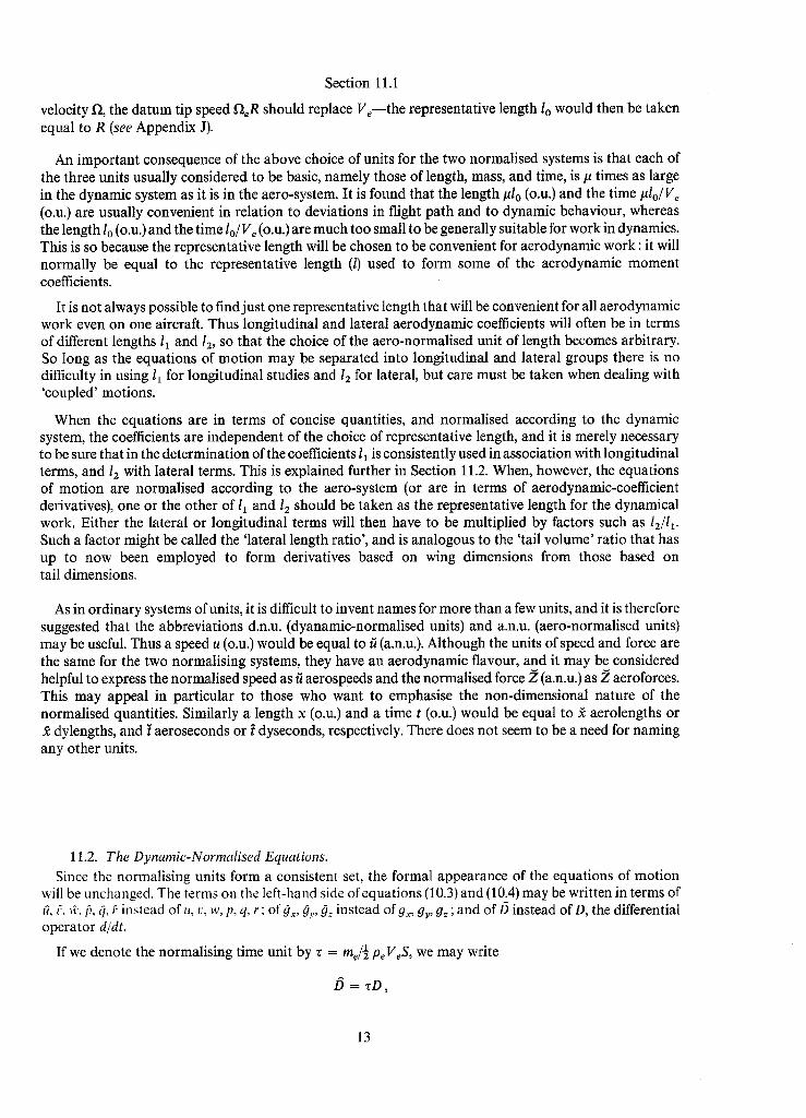
velocity f~, the datum tip speed f~eR should replace V~--the representative length lo would then be taken equal to R (see Appendix J).
An important consequence of the above choice of units for the two normalised systems is that each of the three units usually considered to be basic, namely those of length, mass, and time, is/~ times as large in the dynamic system as it is in the aero-system. It is found that the length #lo (o.u.) and the time I~lo/Ve (O.U.) are usually convenient in relation to deviations in flight path and to dynamic behaviour, whereas the length lo (o.u.) and the time lo/Ve (o.u.) are much too small to be generally suitable for work in dynamics. This is so because the representative length will be chosen to be convenient for aerodynamic work: it will normally be equal to the representative length (1) used to form some of the aerodynamic moment coefficients.
It is not always possible to find just one representative length that will be convenient for all aerodynamic work even on one aircraft. Thus longitudinal and lateral aerodynamic coefficients will often be in terms of different lengths 11 and 12, so that the choice of the aero-normalised unit of length becomes arbitrary. So long as the equations of motion may be separated into longitudinal and lateral groups there is no difficulty in using 11 for longitudinal studies and 12 for lateral, but care must be taken when dealing with 'coupled' motions.
When the equations are in terms of concise quantities, and normalised according to the dynamic system, the coefficients are independent of the choice of representative length, and it is merely necessary to be sure that in the determination of the coefficients l~ is consistently used in association with longitudinal terms, and 12 with lateral terms. This is explained further in Section 11.2. When, however, the equations of motion are normalised according to the aero-system (or are in terms of aerodynamic-coefficient derivatives), one or the other of 11 and 12 should be taken as the representative length for the dynamical work. Either the lateral or longitudinal terms will then have to be multiplied by factors such as 12/l~. Such a factor might be called the 'lateral length ratio', and is analogous to the 'tail volume' ratio that has up to now been employed to form derivatives based on wing dimensions from those based on tail dimensions.
As in ordinary systems of units, it is difficult to invent names for more than a few units, and it is therefore suggested that the abbreviations d.n.u. (dyanamic-normalised units) and a.n.u. (aero-normalised units) may be useful. Thus a speed u (o.u.) would be equal to fi (a.n.u.). Although the units of speed and force are the same for the two normalising systems, they have an aerodynamic flavour, and it may be considered helpful to express the normalised speed as fi aerospeeds and the normalised force ~ (a.n.u.) as 2 aeroforces. This may appeal in particular to those who want to emphasise the non-dimensional nature of the normalised quantities. Similarly a length x (o.u.) and a time t (o.u.) would be equal to ~ aerolengths or
dylengths, and ~ aeroseconds or ~ dyseconds, respectively. There does not seem to be a need for naming any other units.
11.2. The Dynamic-Normalised Equations. Since the normalising units form a consistent set, the formal appearance of the equations of motion
will be unchanged. The terms on the left-hand side of equations (10.3) and (10.4) may be written in terms of fi, :, ~../3, ~?, ~ instead of u, v, w, p, q, r ; of 0x, 0y, 9: instead ofgx, 9y, 9z ; and of b instead of D, the differential operator d/dt.
If we denote the normalising time unit by z = me~ ½ peVeS, we may write
/5 -- ~D,
13

Section 11.2
where/) - d/d~, and the normalising divisors for the other quantities mentioned above are as follows.
Quantity Normalising divisor
U, V,W
p, q, r
g~, gy, g~
Ve
1/T
1 2 Pe Ve S/me
1 2 F o r example, a = U/Ve, p = p~, Ox ~- meOx/½ PeVeS.
When the right-hand sides of equations (10.3) and (10.4) are expanded in terms of force and moment derivatives, it is preferable to normalise these derivatives according to the aero-system (see Section 17). To form a dynamic-normalised concise derivative, such as if%, from the corresponding aero-normalised moment derivative, such as ~w, it is convenient to define inertia parameters ix, iy, i~. These are given by
1 (ix, i,, i,) = ~ (zx, z,, 13,
meto
and are therefore equal to the squares of the aero-normalised radii of gyration. The symbols suggested for the radii of gyration are r,~ ry, r~, so that ix = 5 2, etc.
The multiplying factors required to form the various concise quantities from the appropriate derivatives (in a.n.u.) are given in Table 8. Factors from the third column will yield concise quantities for use with the dynamic-normalised equations. Factors from the fourth column will give concise quantities appropriate for the equations of motion expressed in ordinary units. For example,
- - - - , m w - - i r iyV~z? = V : 2"
The relevant inertia parameter must be used for a moment or a moment derivative: thus,
7v ~Lv uRv
An examination of the Table reveals a pattern that can provide a general basis for determining the multiplying factors for any sort of derivative, including higher-order ones. It is easy to show that for any variable, denoted here by the symbol co, any aero-normalised force derivative such as ~,o will be related to the corresponding dynamic-normalised concise derivative 2,0 according to the equation
:?o, o3
14

Section 1 1.2
TABLE 8
Factors for Converting Forces, Moments , and their Derivatives in Aero-Normalised Units to corresponding Concise Quantities in Different Units
# = me/½ peSlo z = me/½peVeS = #lo/V~
Multiplying factor for forming concise quantity in
Quantity in aero-normalised units
Force
Moment
Force derivative with respect to
linear displacement
linear velocity
linear acceleration
angular displacement
angular velocity
Moment derivative with respect to
linear displacement
linear velocity
linear acceleration
angular displacement
angular velocity
Example
~ g
,,#o
~h
2w 2, 2.
~h
~w
dynamic-normalised units
- 1
- ~ / i y
- 1
- 1
--#2~Jr -IViy
- 1 / i y
- ~ / i y
- 1 / i r
ordinary units
- V e / ~
-- ~/ilc 2
_ ~ / ~ 2
- - 1 / z
-1/#
- V e / ~
- V d t ~
- #2/iyVez3
- #/iy Vez 2
- 1/i, Vez
- - ~ / i y q ~ 2
- 1 / i f i
Similarly rh,o # 63 J~a~ = iy (b"
The ratio cb/6) depends only on the dimensions of 09, and is a power of # as given by the following Table (second column).
It can also be shown that the concise derivatives in ordinary units are related to the corresponding dynamic-normalised derivatives as follows :
o o z___~ = V e cb __m~' = 1 6) i~o z e 3 ' ~ ~2&,
15
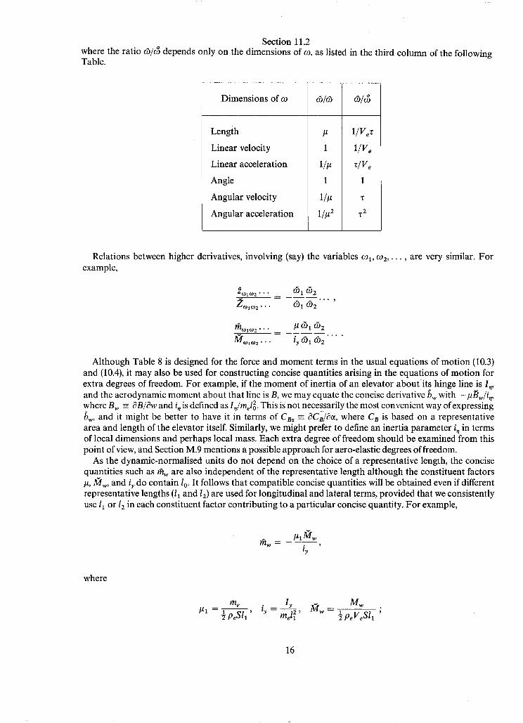
Section 11.2 where the ratio th/e] depends only on the dimensions of co, as listed in the third column of the following Table.
Dimensions of co
Length
Linear velocity
Linear acceleration
Angle
Angular velocity
Angular acceleration
~/~
#
1
1
1/#
1/# 2
~/o5
1/VeZ
1/V~
T/Ve
1
,~2
Relations between higher derivatives, involving (say) the variables col, 0)2 . . . . . are very similar. For example,
Zo~0~2 ' " d ) t ~32 " " '
rh,o~,o~ • . . # °31 o32
/~m1¢o2 " ' " iy {~)1 ~)2 . . . .
Although Table 8 is designed for the force and moment terms in the usual equations of motion (10.3) and (10.4), it may also be used for constructing concise quantities arising in the equations of motion for extra degrees of freedom. For example, if the moment of inertia of an elevator about its hinge line is I,, and the aerodynamic moment about that line is B, we may equate the concise derivative bw with -i~Bw/i,, where Bw - OB/~w and i~ is defined as l,/mel 2. This is not necessarily the most convenient way of expressing bw, and it might be better to have it in terms of CB, - OCB/be, where CB is based on a representative area and length of the elevator itself. Similarly, we might prefer to define an inertia parameter i, in terms of local dimensions and perhaps local mass. Each extra degree of freedom should be examined from this point of view, and Section M.9 mentions a possible approach for aero-elastic degrees of freedom.
As the dynamic-normalised units do not depend on the choice of a representative length, the concise quantities such as rh w are also independent of the representative length although the constituent factors #,/~tw, and iy do contain lo. It follows that compatible concise quantities will be obtained even if different representative lengths (11 and/2) a r e used for longitudinal and lateral terms, provided that we consistently u s e 11 o r l 2 in each constituent factor contributing to a particular concise quantity. For example,
#1-/~w iy
where
m e
#1 ½ peSll l y M w
i, = - ~ , ff/I~, = ½ pT-V-~SI 1 ;
16

Section 11.2
and
P2~o ix
where
me I~ N~ ~2 = ½ peSl 2 iz = ..--.-.-.-.-.-.-.-~, ~[v -- ' reel2 ½ peVeSl2 "
The above remarks also apply to the concise quantities in ordinary units, but not to concise quantities normalised according to the aero-sYstem.
11.3. The Aero-N ormalised Equations.
As stated previously the aero-normalising units of length and time are not generally suitable for dynamic analysis. It may occasionally, however, be desired to employ the equations of motion normalised according to the aero-system, and these are obtained as follows.
The terms on the left hand sides of equations (10.3) and (10.4) may be written in terms of ~, ~, #,/~, ~, r- g:,, gr, #z, and of the operator i3. Since the unit of time is of magnitude lo/V~, we have V~/3 = loD, where D = d/d~, and the n6rmalising divisors for the other quantities are as in the following Table.
Quantity .Normalising Divisor
U~ I)~ W
p, q, r
gx, Or, g~
ge
Ve/lo = p/z
V~llo = I~peV~S/2me
For example, ~ = u/Ve ( = a), ~ = plo/V ~ ( = p/p), gx = m~gff½ P e V 2 S ~ ( : ~x/#)" When the aircraft mass and moments of inertia are constant their values in aero-normalised units are
/~e : ]l, and ix -- #ix, etc. It follows that all concise quantities concerned with aerodynamic forces can be obtained by dividing by - p , and all concise quantities concerned with aerodynamic moments can be formed by dividing by -pix, - # i r, or -pi~, whichever is appropriate. For example,
~o = - : g e / , , ~ = - # i w / , i , ,
When different representative lengths, say 11 and 12, are used for longitudinal and lateral aerodynamic coefficients, and for their derivatives, one of these should be chosen as the aero-length for normalising the equations as a whole. This naturally includes the expressions for # and the inertia parameters ix, iy, ix, etc.
12. Stability and Response Quantities.
It is convenient to have symbols for representing the complicated determinantal expressions that arise when we are studying the stability and response of an aircraft on the basis of small perturbations and linearized equations of motion. As examples we have taken the separate groups of longitudinal and lateral equations as set out in Section 10.2.3, and in each case we first consider the natural aircraft, that is the aircraft in a state where motivators are not actuated by any automatic control device.
17

Section 12
We distinguish between the operator D = d/dt and the Laplace transform or Heaviside parameter. It has been traditional to represent the latter as p in non-aeronautical work, although the strong influence of American literature on automatic control is resulting in the use of s. It is not advisable to use p in aeronautical work since it represents rate of roll, and the use ofs is generally endorsed. There may occasion- ally be a clash with another s, for example the pilot's control output (see Section 8), and in principle it seems unnecessary as a rule to depart from the traditional 2, for its original meaning of a root of the stability equation is consistent with Laplace parameter usage. In this report we use 2 but the freedom of choice exists to suit the circumstances. The incidence-plane angle is also denoted by 2, but this would rarely cause any confusion.
12.1. Longitudinal Stability and Response. If only one type of motivator is in operation (say the elevator), equations (10.12) and (10.14) may be
reduced to the operational form
u' w' q' 0 h' t/ (12.1)
A.. A~. Aq. D- 1Aq. Ahn A 0 '
where the denominators are polynomials in D, and are equal (apart from sign) to the determinants formed from the array below by deleting each column in turn. As it stands the array is valid for level flight (Te = 0), but can also be applied to non-level flight in a uniform atmosphere by putting Xh = Zh = mh ---- 0, and replacing h' in equations (12.1) by - z ~ , Ah~ becoming - A~,.
t D+x. x.D+xw (Xq-Jc'We) D-.l-g 1 x h x .
z. (1 +z . ) D+z~ (zq-u~) D+g2 zh z,
m. m.D + m~ D 2 + m.D mh m.
- sin ~e cos ct e - V e D 0
It is useful to express each denominator of equations (12.1) in the form
A., = Uxx, + Uzz, + U,~% , (12.2)
since the twelve polynomials Ux, Uz, Urn, W= etc. recur in the analysis of aircraft stability with and without automatic control. A,, may be called the complete response polynomial of u with resPect to q, and it has component parts Ux, Uz, Urn, which are response polynomials.
The function Ao, obtained from the first four columns, defines the stability of the aircraft when the motivator is fixed, that is ~/' = 0. If in the usual way we assume that u', w', q', O, h' are proportional to exp(2t), and we replace D by 2, the equation Ao = 0 becomes the characteristic or stability equation for the natural aircraft, and Ao is called the stability determinant or (after expansion) the stability polynomial*. The polynomial is in general a quintic, and the determinant may be expanded in various ways, such as
Ao = Ux(2 + x.) + W~(x.t + xw) + Q~[x~ + we + g l;~- 1] + H~xh
= U~z, + W,[(I + z~)l + zw] + Q~[z,-. u e + g22- ~] + H, zh.
= U,nm u + Wm(m•2 + row) + Qm(2 + m~) + H,.mh.
*The stability determinant for any system may be denoted by A. The suffix o is added here in order to avoid confusion later in this Section, but may be omitted when no confusion arises. Similarly, Au may be written instead of A~ when possible, and expressed as a polynomial with coefficients Ui: A, = E UiD ~.
i
18

Section 12.1
If
A 0 = K s l S + K 4 2 4 + K s 2 3 + K 2 2 2 + K 1 2 + K o ,
and Umi, etc. are the coefficients of 25 in the polynomials U,~, etc., distinct expressions for the coefficients Ki may be obtained from the various expansions of Ao. The third expansion, for instance, leads to the following expressions.
K s = Qm4
K4 = Qma + Q,~4rn~ + Wmam,
K3 = Qm2 + Qm3mq + Wra2mw "Jr- Wmam w + Um3m u
K2 = Qml + Qm2m~ + W m l m , + Wm2mw + Um2mu + H,~2mh
K1 = Qmtm~ + Wmom, + Wmlrnw+ Umtm,+ Hmtmh
K 0 = Wmom w + Umornu + Hmomh
A complete list of the coefficients Umi, etc. is given below. Extensive use is made of short-hand expressions for second-order determinants: for example,
XuZw-- XwZ u =_- XuZ w ,
and it is suggested that the overscript "-. be called a 'slur'.
Ux4 = 1 q-z,~
Ux3 = mq + Zw + Uem~, + mqz,
Ux2 = Uem w + mqz w - g2mw - z h cos O~ e
U xl = - g 2mw + V e( mhzv¢ + W ernh) + mhz ~ cos ote
Uxo = Ve~hz w-I- g2mh cos t~ e
Uz4 : .- x~
Uza = -- x w "mqx~, -F Were ~,
U~2 = mwx,j + wemw + g t m , + xh cos ~e
U~I -- #lmw + Vem~,Xh +(mClXh -- w~mh) cos ~
Uzo = VemwXh--glm h cos ~e
19

Sec t ion 12.1
Urn3 = - - x q - - w e "-[- ~qX w - - UeX~i , - - WeZ¢,,
U,.2 = x~zq - ,qx(1 + z . ) + 9 z x . - uex. , - wez ..
U ,. ~ = - g ~ zw + o ~ x . , + Ve( ;'gwZ, - - W .X~) + ( ~ Z ~ + W ~Z~) COS ~
Umo = V~x"~wzh + (91Zn-- 9zXh) COS ~
W x 3 = _ z u
W x 2 -~. - t~qz u - Uem u - z h sin ¢x e
W x t = f l 2mu + (m'~hZq - - Uemh) sin ~z,
W ~ o = V~m"~h + gzmh sin ~
W z 4 -~- I
W z 3 = x u + m q
W z 2 = X ~ ' ~ q - - W e m u + x h sin ~e
W z t = - 91m,, + VeUem h + m"qX h sin 0~ e
W z o = V e m ~ x . - - g t m h sin (x e
Vl/m3 ~ bl e - Zq
W, .2 = u~x~ + w~z~ + z~xq - 92
W , . 1 = ,q ~ z . - 92 x,, - V~uezh + ( x ~ h + UeXh) sin 7~
W . , o = V ~z"~h + (91zh --.q z Xh) sin c~
Qx3 = - mu + n~,Zu
Qx2 = ~h~wz,, + (mT~,zh - mh) sin ~e
Oxl = m"~h cos ~ , + m ~ , z h sin ~
Qz3 = - m w - m~'x ,
Q~2 = - m,v"x, + mh cos ~e + m~'x+ sin ~x e
Q z l = ll~hXu COS ~e + m ~ w sln~x e
20
Section 12.1
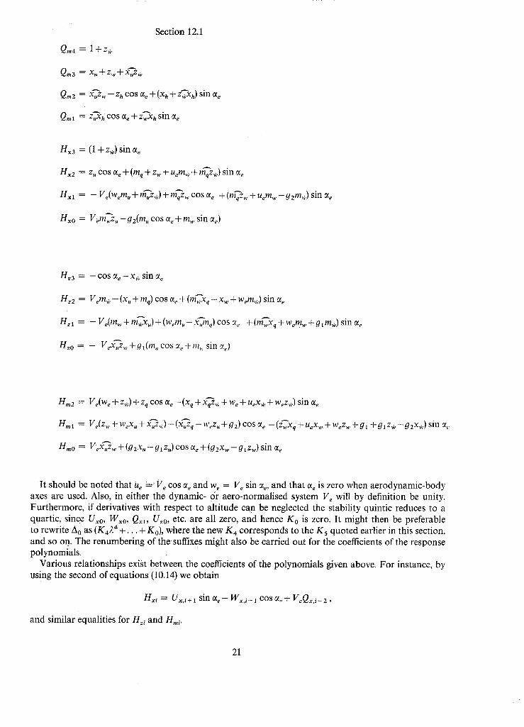
Qm4 = 1 + z~i.
Qm3 = xu W zv,,'-l- x " ~ ,
Q,.2 = x'-~w - Zh COS ~ + (xh + z~'~h) sin ~e
Q,.~ = z'~h cos ~ +z~xhsin ~e
H~3 = (1 +z~) sin ~e
Hx2 = z u COS ~e + (mq + z w + u~m,+ + ~-~qz.,) sin ~e
H x l = - V e(wemu + @~i,) + m'-~w c o s ~e + (tT/~w + Uemw - ,qzm~) sin ae
H~o = V~n~.z . -g2(m. cos a~+mw sin a~)
Hz3 = - c o s ~e - - Xff s i n ~e
H~2 = Vem¢,, - ( x . + mq) cos ~ + (m~.xq - xw + w~m~O sin ~e
H~ I = - V ~(mw + m ~ c . ) + (w d n . - X~nq) cos ~e + (m~xq + Wemw + ,q 1 m . ) sin ~
Hzo = - V~x"~w +,ql(m, , cos :~,. + m,,, sin ~ t
H,,, 2 = V.(we + z~,) + zq c o s a e - (Xq + x " ~ + w e -[- bleX ~ + WeZ~i, ) sin a~
Hm I = Ve(zw -t- WeX u q- .~i.~.) "+" (XP~q -- WeZ u -'1- g Z) COS O~ e -- (~w.¥q' "Jr- UeX w + WeZ w + g 1 + .q 1Zfv -- O 2X~. ,) sin c~,,
H/~ 0 = V ; x " ~ + ( 9 2 x , - Olz , ) cos ae + (.qaXw - 9 lzw) sin ae
I t should :be noted that Ue ----" Ve cos ae and w e = Ve sin ee, and that ae is zero when aerodynamic-body axes are used. Also, in either the dynamic- dr aero-normalised system Ve will by definition be unity. Furthei:more, if derivatives with respect to altitude can be neglected the stability quintic reduces to a quartic, since Ux0, Wxo, Qxl, U~0, etc. are all zero, and hence Ko is zero. It might then be preferable to rewrite A0 as (K424+. . . + K0) , where the new K4 corresponds to the K5 quoted earlier in this section, and so on. The renumbering of the suffixes might also be carried out for the coefficients of the response polynomials.
Various relationships exist between the coefficients of the polynomials given above. For instance, by using the second of equations (10.14) we obtain
Hx~ = Ux,~+~ sin a e - W x , i + l cosao+ VeQx,i+ 2 ,
and similar equalities for Hz~ and H,. v
21

Section 12.1
Automatic control.
Consider an automatic pilot which produces pitcher, proaptor, and catanator deflections (see Section 8). Ideally simplified linearized control equations would be of the form
!
q' = GuU' + G~,Du' + Ga ~ u + Gww' + . . . . . .
h 1 , i v' = Auu' + A~,Du' + ~, -~ u + Aww + . . . . . .
! i x' = Cuff + C¢,Du' + Cr,-D u + C~,w + . . . . . .
where G,, A., C,, etc. are autopilot parameters* (called gains or gearings), which are assumed constant for small deviations from particular steady state flight conditions, but which may be varied as functions
t t ~
of the steady state flight conditions. The operator lID is defined to be I ' ' "dr. It is sufficient to consider J
the abridged control equations. 0
~l' = Guu' + Gww' + GoO + Ghh' ,
v' = Auu' + A~,w' + AoO + Ahh' , (12.3)
t¢' = Cull' + Cww' ' + CoO -1- Chh' ,
since the effect of other gearings can be deduced as will be explained.
When the motivator deflections are functions of the variables it is possible to derive many expressions on the lines of (12.1) giving the ratios of pairs of variables, and it does not seem necessary to devise a notation that would cover all possibilities. It is, however, useful to consider the stability polynomial, which from equations (10.11), (10.13), and (12.3), is equal to the determinant A given by
a 1 a 2 a 3 a 4 X v Xn X~
bl bE b3 b4 zv g n gr
cl c2 c3 c4 my m, mr
dl d2 da d4 0 0 0
- A n - A w - A o --Ah 1 0 0
- G , - G w - G o --Gh 0 1 0
- C u - C w - C o --Ch 0 0 1
w h e r e [alb2c3d4l would be the stability determinant (Ao) when v' = ~/' = x' = 0, as set out earlier in this Sectiofi. The general expression for A has the form
* Other suffixes (or no suffixes) may be used when control equations include awkward transfer functions
or special groupings. For example, r/' 1 + nzD GO ~l' = l + z D or = Gl(O+kh')+ I-FZ13 G20"
22

Section 12.1
A = A o + A u Auv + Aw Awv + AoAqfl- 1 + AhAh ~ +
+ GuAu, + GwAw,7 + GoAq,/. + GhAh n +
+ CuAu ~ + Cu, AwK + CoAq~) ~- 1 + ChAh K +
+(double product terms such as A.G . . . . . )+
+ (triple product terms such as .4.,G,,C,... 3.
and the first three rows may also be put in the form
A0 + xv(AuUx + AwWx + AoQx 2- l + AhHx ) +
+ z,.(A.U: + A..W: + AoQ:2- ~ + AhH:) +
+ m~(A. U,. + A~, W m + AoQ,,.2-1 + AhHm) +
+ x,(G.Ux + G~,Wx + GoQx2- ~ + GhH~,) +
+ z,(G.Uz + G,vW~ + GoQ~2-1 + GhH~ ) +
+ m~t(GuU m + GwW m + GoQ,.2-1 + GhH,.) +
+ xdCu Ux + Cw W~ + CoQx2- ~ + ChH~) +
+ z~(CuU~ + CwW~ + CoQ:2- ~ + ChH~) +
-4- mJ C,, U,,, + C.. W,,, + CoQ,.2-1 + ChHm )
When there is only one kind of control all the double and triple product terms are zero as well as many of the simpler terms, since only A's or only G's or only C's are involved.
The triple product terms are all contained in the product of two determinants :
XO X v X K
Zq Z v Z r
m . m y m~
x - s i n :%
- G u
- A .
- C u
cos ae - V e )L
- G., - Go - Gh
- A w - A o --Ah
- C ~ - C o --Ch
The contribution to the stability polynomial is therefore equal to
(mS& + + + + ¢.4,,C,,.)+
+ r e ( . . . . . .
+oos o( . . . . . . ) + c,, ,@,, + ¢ . .@, , j+
+s in ae( . . . . . . )(G,,.AoC,,+GoAhCw+G,,A,,.Co).
The double products are conveniently listed in terms of second-order minor determinants of Ao. The eighteen minors required are those containing elements of the fourth row, and each minor occurs in three double product terms. The 54 terms may be obtained from Table 4. Thus, the contribution to the stability polynomial is given by Table 4A :
23

GhAo
GhAw
GoAw
G.A~
G.Ao
G,,,A.
t l l , I X ~.
GoAh
G,,,Ah
G,,,Ao
GhA,,
GoA
G,.,A.
XvZ~ I ZvtHn
AoCh
A,~,C h
A,,,Co
AhC,,
AoC.
A.Cw
GhAo
GhA.~,
GoA w ,..., G,Ah
~f~_Ao I
G ,,.A.
Section 12.1
TABLE 4A
Xvln~¢ XvZ~ ¢
AhCo
AhC,,,
AoC.,
AuCh
A ~C o . w-"~
AuC,,.
AoCh
A,~,Ch
A ,,, C o
AI, C,,
AoC~
A~C,,, 1
I
tll~lZu. DI~IX K
CoG~,
C,,.G~
C.,Go
ChG,,
COG,,
C.G,,,
C~,Go
ChG,,,
COG,,,
C.Gh
C.Go
C.Gw
ZK.'(rl
a 1 d2
a3dl 1211 d 4
(.13d 2 1-,,
a2d4
a3d4
bid2
b3cll w".,
bld~
b3d:
b 2d_~
b4d3
ChGo ('l d2
ChGw (~'3dl CoGw c ld.~
C,,Gh c3d 2
CuG 0 12'2d4
C,,,G,, c 3d. +
+ ,,,,,~, ( ¢,~,,h,~N~ + oTA~h~, + . . . . . ) +
+ x,~. (o.'%,c,12-~2 + ohm,, <~, + . . . . . )+
÷ . . . . . . . +
+ z~"?x, ( C"~octd2 + . . . . . . . . + C~G.c~t4) are the required terms.
It should be noted that each gearing product such as Gh"Ao occurs once in each block. Table 4B gives the complete expressions for the minors. For example,
aid4 = 22 + x~2 + xh sin % .
As an example consider an autopilot whose equations are
~7' = GoO , v' = A u u ' , tc' = C h h ' .
24

Section 12.1
T A B L E 4B
a f t ,
a3dl
a i d4
a~12
a2d4
a3d4
.7--- bid2
badj
bld,
b3d2
b2d4
b4d3
(' 1 d2
c3dt
c~dz
c~d2
c2d4
c 3 d 4
23 coeff. /~2 coef f .
X¢.,
We W Xit
1 +z~ ,
bl e -- Zq
- s in ae
COS ~e
mff
mq
2 coeff.
cos ae + x , sin ~e
V~-(w~ + xq) sin e~
Xu
VeX, # + (W e + Xq) COS ~X e
Xw
gl
(1 +Zw) sin ~
(u~ - zq) sin %
Zu
V e(1 + zvi, ) -- (u e -- Zq) COS ~e
zw
- -92
mw sin c~ e
--mq sin c~ e
mu
Vem.iv "t" Wlq COS ~e
1~flu,
Const. coeff.
X u COS ~e + Xw s i n ~e
VeXu--gl sin ~.,
Xh sin c~ e
Vexw + g I COS Ce e
- - X h COS ~e
V~Xh
zu cos ae + zw sin ~e
V e z u - g2 sin ~e
Zh sin ae
Vezw + g2 COS ~x e
-- Z h COS C~ e
-- Vez h
m, cos ~e + mw sin Ue
Vemu
mh sin c~ e
Vemw
- m h c o s ~e
Vemh
The stability polynomial is
A = A o + Go 2- l(Qmm,1 + Q~z, I + Qxx,~) +
+ A,(Umm~,+ Uzzv+ Uxxv)+
--[- C h (H,,,m,~ + H~z,, + Hxx,,) +
+ GoAu(<X,.b94-t~z~a~d4 - ~znc~d4)"t-
+ A.c, ( - x5~c~2- z.7.~.3~2 + x,mKb74) + + GoC~ (-- m"&a~2 + ,Z~b-)2 ÷ ;&c~ 2)- - GoA,Ch cos c~, (m,x~'-'z~ + zn~'~x~ + x,z~'~m~).
If the pitch control equat ion is instead
q' = GoO + Gqq',
25

Section 12.2
we merely have to pick out all the G o termsin the expression for the stability polynomial and write (Go + Gq2) 1
wherever there is a Go. Similarly if the control equation contains a term Go-~ O, we must add Go2-1
wherever there is a Go.
12.2. Lateral Stability and Response. If only one type of motivator is in operation (say the ailerons), equations (10.13) and (10.15) may be
reduced to the operational form
v' p' q~ r' 0 Y~ ~' Ave Av~ D- 1Av ¢ A~¢ D - t Ar¢ Ay~ A o (12.4)
where the denominators are polynomials in D, and are equal (apart from sign) to the determinants formed from the array below by deleting each column in turn.
( D+y~, (yp-we) D - g 1 (y~+ue) D - g 2 0 y~ \
Iv D 2 + IpD exD 2 + l,D 0 I¢ ) n, e:D z + nnD D 2 + n,.D 0 n¢
- 1 V,, sin ~,, - V,, cos ~,, D 0
As in Section 12.1 we express the denominators of equations (12.4) in the form
A r c = Vyy¢ + VII" ~ + Vnn¢, (12.5)
where A,.~ is the complete response polynomial of v with respect to ~., and its component parts V,., V~, V, are response polynomials. The footnote on page 18 also applies here, so that for example we may write A~¢ = A~ = ~ V~ D * if there is no ambiguity.
i
The stability determinant A 0 is obtained from the first four columns. The stability polynomial is in general a sextic with a factor 21 corresponding to the neutral stability of an aircraft (when no control is applied) in respect of
(a) lateral deviations from the datum flight path,
(b) angular deviations in heading from the azimuth datum.
The determinant A o may be expanded in various ways, such as
Ao = Vr(2 + Yv) + Vllv + V,n~
= Py(Yp- We- 912-1) + Pi(2 + Ip) + P,(ez2 + np)
= Ry(y r + Ue _ ~q2/~ - 1) "b" Rt(ex2 + lr) + R,(2 + n¢).
If A 0 = J626 + J52s + J424 + J323 q- J2~, 2 ,
and Vyi, etc. are the coefficients of 2 ~ in the polynomials Vr, etc., distinct expressions for the coefficients Jg may be obtained from the various expansions of Ao. The first expansion, for example, leads to the following expressions.
26

Section 12.2
J6 = Vy5
J5 = Vr4 + VysYv
J4 = Vy3 + Vr4Yv + Vt4lv + V .4nv
J3 = + Vr3yv + V n l v + Vn3nv
J2 = Vl21v + Vn2nv
A complete list of the coefficients Vy~, etc. is given below, and as before the 'slur' is used to shorten the writing of expressions such as
Vy5
Vy4
vy3
g l4
El3
Vt2 =
Vn4
Vn3
Vn2
Py4 =
Py3
El5 =
e l 4 =
Pt3 =
Pt2 =
P.5 =
/° .4 =
Pn3 =
Pn2 =
Yy4.
Yr3 =
Yy2 =
Vy 1 =
lvn r - Irtl v = l ~ r •
= 1 - - exe z
= Ip + n, - exnp - ezI,
= Ip~l r
w~ - yp + e~(u~ + y~)
Uenp -~ Wenr + Y~'~p ~- 01 -- ezO2
g l n r - - g 2 n p
- - (u e + Y~) -- e~(w e -- yp)
- - uf lp - - wfl~ - - y f lp + g2 - - e~g 1
g21p- -g l l r
- 1~ + exno Ry4 = -- no + ezl .
lrrlv Ry 3 = Ivn p
1 RI5 = - - e z
Yv + nr Rt4 = - - n p - - e~y~
yvtlr -- Uerl v Rl3 : ypl'l v -- Wen v
g2nv Rl2 = - - 9 1 n v
- e x R .5 = 1
- l ~ - e~y~ R . 4 = y~ + Ip
y~l~ + u~lo Rn3 = yoIp + w fl~
- 9 2 1 v R . 2 = g11v
1 - exez = Vr5
lp + n ~ - e ~ n p - e~l~ = Vy 4
lpn~ - u,(n~ - e fl~) + w~(lo - e~no)
Uelvnp + Welvnr
27

Section 12.2
Yl3 = - Yp + e~yr
YI2 = f ' ~ p - - yv(We + ezUe) + g 1 - - ezg2
Yt~ = - UeYvnp - WeYvn~ + g a nr - g znp
Yto = - Vegn~ cos ?e = - n~(91ue + g2we)
Yn3 = - - Yr + exyp
Yn2 = yplr + yv(Ue + exWe) + g 2 -- ex91
Yn 1 = UeYvlp d- weyol r -- g 11r + g21p
Yno = Veglv cos 7e = Iv(91Ue +9zWe)
It should be noted that if aerodynamic-body axes are used then u e may be replaced by V e, and w e equated to zero, since U e = V e cos ee, we = Ve sin ee. Also, in either the dynamic- or aero-normalised system V e will by definition be unity.
Various relationships exist between the coefficients of the twelve polynomials. For instance, from the third of equations (10.15) it follows that
Yy l = V r , i + l - w e P y , i + 2 + u e R y , i + 2 ,
and similar equalities are found for Yu and Yni.
Au toma t i c control.
Consider an automatic pilot which produces roller, dexilator, and yawer deflections (see Section 8). Ideally simplified linearized control equations would be of the form
, 1 , ~' = Fvv' + F ~ + Fo -~ v + F j p + . . . . . .
, 1 , 5' = Bvv '+Bob +B~-D V +BcqS+ . . . . . ,
1 , ~' = Hvv' + H~f)' + H~-D V + Hvdp+ . . . . . .
where F~, B~, H~, etc. are autopilot parameters* (called gains or gearings), which are assumed constant for small deviations from particular steady state flight conditions, but which may be varied as functions of the
t t'*
state flight conditions. The operator 1/D is defined to be .|...~ dt. It is sufficient to consider the steady
abridged control equations
7 ¢' = F y + F ~ck + Fog, + F,y~ , 1
6' = Bvv' + B4,c~ + B o ~ + Bry + ,
~' = Hvv' + H4~q~ + HO~ + H y y ~ ,
since the effect of other gearings can be deduced as explained in Section 12.1.
(12.6)
*See footnote on page 22.
28

Section 12.2
As in the longitudinal case all possible relations similar to equations (t 2.4) are not considered when the control applications are functions of the variables, and only the stability polynomial is set out. The
at a2 a3 0 y~ yo y~
bt b2 b3 0 I~ I~ l~
C l C 2 C 3 0 n~ n~ n~
dt d2 d3 d4 0 0 0
- F v - F~ - F , - F r 1 0 0
- B v - B¢ - B , - By 0 1 0
- H v - H 4, - H ~ , - H y 0 0 1
stability determinant A is
where [atb2cad4] would be the stability determinant Ao when ~' = 3' = (' = 0, as set out earlier in Section 12.2. The general expression for A has the form
A = Ao + FvAv¢ + F~Ap~2- t + FoA,¢2-1 + FrAy ¢ +
+ BrAy ~ + BeAch2-1 + B~A~2- t + BrAy ~ +
+ HvAv~ + Hc, Ap~2- ~ + H~,Ar~2- t + HrAy ~ +
+ (double product terms such as F ~ B , . . . ) +
+ (triple product terms such as F~.BcH~.. .) ,
and the first three rows may also be put in the form
A0 + y¢(Fv Vy + F~Pr2- x + FoRt 2 - t + Fr Yr) +
+ l¢(FvVt + F~Pt2- t + FoRt 2 - t + Fyy t ) +
+ n,(FvVn + F~,Pn2- t + F~,Rn2- t + FyYn ) +
+ y~(B~, V~. + B4,P~,2-1 + B,I, Ry 2 - 1 + By Yy) +
+ I~(BL. V l + BcP~2- 1 + BoRI 2 - 1 + B.~, Yt) +
+ n~(B,.V, + Be)Pn2-" 1 + BoR,.; t - 1 + ByY~) +
+ y~(H~, Vy + H4,Py2- 1 + HoR f i - ~ + H,. Y.,,) +
+ lr.(H~,V I + H~,P~2 - t + HcR~), - 1 + Hyyl ) +
+ n:(H..V,, + H,t,P,2- 1 + H,I,R, 2 - 1 + Hf f , , ) .
Where there is only one kind of control, all the double and triple product terms are zero as well as many of the simpler terms, since only F's or only B's or only H's are involved.
The double products are conveniently listed in terms of second-order minor determinants of la~b2c3d4l. The eighteen minors required are those containing elements of the fourth row, and each minor occurs in three double product terms. The 54 terms may be obtained from Table 5. The contribution to the stability polynomial is given by Table 5A.
29

Section 12.2
TABLE 5A
lcn~ ygn¢ y¢1¢ lena Y6n~ yolg long yon~ yoI¢
Folly FoBv BoHy aid2
F~Hr FeBr B,Hy aad 1
F ,H , FoB o Bc~H o a ~d4
FvH,, FyBo BrH~ aad 2
FoH~ F oB~ BoH~ a2d,~
F~.H¢ FvB o B~.H4, aad,
Folly
F¢Hy
Foil, F~Hy
F~,Hv
F~,H ,
FoBy ByH 0 bad2
F 4,By BvH ¢o bad 1
FeB o B ,H, b~d4
FyBv BvH v bad2
FoBs. BvH o b 2d,,
F~,B, B¢,Hv bad,,
FvH, FyBq, B,Hv cld 2
FeHy ForBy ByH¢ c i d 3
F,Ho F4,B o Boll ~ c4dt
Frill, FyB,, BvHy c2d s
FvH, F,.B o BoHv c2d4
Fc, H,, F'g~B~ BvH ~ c3d, ~
+ y~n¢ (F~HrbTd 2 + F~Hyb3da + . . . . . )+
+ y¢l~ (FyH~cld2 + FcHvcad 3 + . . . . . )+
+l¢na ( FoByaad 2 + F¢Bra3d x + . . . . . )+
+ y~l¢ (B,'-'Hycl~2 + . . . . . . + B~,H,c'fl4) are the required terms.
It should be noted that each gearing product such as F~'Hy occurs once in each block. Table 5B gives the complete expressions for the minors..For example,
A
bid2 = ,I, 2 + Iv2 + lvV e sin ~te.
30
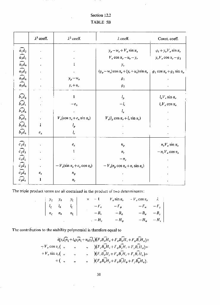
Section 12.2
T A B L E 5B
ald2
aadl
aid4
a3d2
a2d4
aad 4
btd2
b3dt
bld4
bad2
b2d4
bad4
¢1d2
Cld3
c4dl
c2da
c2d4
cad4
2 s coeff. 2 2 coeff. 2 coeff. Const . coeff.
1
ex
e z
1
yp -- W e -[- g e sin t~ e
V e c o s ~e -- Re -- Yr
Yv
gt +y.V~ sin c~ e
yvVe COS 0~e-- ~2
yv -- w e
Yr + Ue
1
- - e x
Ve(cos ae :4- ex sin a~)
Iv
e~
1
- V ~ ( s i n ~e + e= c o s ae)
lIp
lIe
(Yp- we) cos ae + (Yr + ue) sin ae
gl
92
Ip
- - I r
Ve(lp cos o~, + Ir sin O~e)
l I p
lIt
D ?l v
~1 :COS (Xe "~- g2 sin 0%
IvV e s in ae
lvV e COS 0~ e
- Ve(% cos ae + n, sin ae)
nvV e sin ~ e
-- II t, V e COS ~e
The triple p roduc t terms are all contained in the product of two de terminants :
Y~ Ya Y¢ I¢ 1~ I;
?1¢ n a n~
- 1 V~ sin a~ - V~ cos a~
- F~, - F , - F o
- B~, 2_ B , - Bo
- H,, - H ¢ - H ,
The contril~ution to the stability po lynomia l is therefore equal to
).(y fl"~¢ + l oy~¢ + nS'J¢)( F,,B~H O + F eBTH ~ + F oB~H,~ )+
+ V e cos u~.( . . . . . . )(F,BoH r + F4,B.,.H. + FyB,.ff,)+
+ V~sin c%( . . . . . . )(F,B,H.,.-~-F~,B.,H.+F.,B,Hp)+
+( . . . . . . )(F4,BTHy+F,B~H,+F~.B~'~Ho).
2
- - Fy
- B y
- H y
31

As an example consider an autopilot whose equations are
~' = F , ¢ , 6' ?= Bvv',
The stability polynomial is
A = A o + F , 2 - S(pyy~ + P~l~ + P,n~) +
+ Bv(Vyyo + Vtl ~ + V,na) +
+ H , 2 - l(Ryy¢ + Rtk + R.n~) +
+ FoBs(- l~n~aad 4 - y~n~b3d4+ y,l~c3d4)+
+ B,H o ( - l,n~a 2d4 + yen;b 2d4 - yol~c2d4) +
+ F,Ho(l~n~a i d, + y~n~b t d4 + y;l,c4d l) -
- F,B~H,2(y~kn ~ + l~y~n~ + n~y~l~).
If the roll control equation is instead
(' = H~ ,~ .
~' = F , ¢ + Fpp',
we must pick out all the F , terms in the expression for the stability polynomial and write (Fv,+Fp2)
F__ 1 wherever there is an F~. Similarly if the control equation contains a term * D q~' we must add F~2-1
wherever there is an F, .
13. Some Characteristics of Linear Dynamic Systems. 13.1. General Nomenclature.
The behaviour of many* linear systems can be specified in terms of a set of differential equations
AO X a b = A~5~ + Axfb + . . . + F~,
f a b Aoy = Ay6o + Aj) b + . . . + Fy, (13.1)
and so on, where x, y . . . . are the variables; 3,, 3b . . . . represent control inputs such as motivator deflections ; Fx, F~, . . . . are disturbances ; and the A's are polynomials in the differential operator D =- d/dt and having constant real coefficients. Any one of these equations may be derived by eliminating the unwanted variables from the original equations of motion, and the same polynomial A o will always be obtained on the left-hand side. Certain coefficients are given special names, and before considering the overall equations** of motion (13.1) we deal with a simple second-order equation
a 2 + b 2 + c x = F , (13.2)
*A report on notation does not seem a suitable place for dealing with the characteristics of a general linear system. There are many books covering this ground, for example Brown 32. There appears to be no standard term for linear differential equations with constant coefficients, but the name 'panlinear' has been proposed33.
**This term and others defined later were introduced in Ref. 34 in order to clarify the interpretation of certain properties of panlinear systems.
32

Section 13.1
where x represents a linear or angular displacement. By analogy with a system comprising a mass, dashpot, and spring, we may call the three terms on the left-hand side the inertia term, damping term, and stiffness term. The coefficients a, b, c, respectively are named in the same way.
When we have two second-order equations in x and y, we can give useful names provided the variables have been chosen in a special way, and it is usual for this to be done. Consider
ASi + BYc + C x + l ~ + m p + n y = F~ ,
J a £ + b Y c + c x + L ~ + M p + N y = Fz. (13.3)
In general these equations are called the F1 and F 2 equations, and F1, F 2 might for example represent forces in two particular directions, whereas x, y might represent deflections in other directions. This procedure is unusual, and it is normally profitable to associate F1 with the x direction, and F2 with the y. This is also convenient for nomenclature, for we may then call A and L the direct inertia coefficients, and a, 1 the cross inertia coefficients. Similarly, B and M are direct damping coefficients, b and m are cross damping coefficients, C and N are direct stiffness coefficients, c and n are cross stiffness coefficients.
When F1 is associated with the x direction the terms AS~, BYe, Cx and l~, my, ny in the F1 equation are called direct terms and cross terms respectively, and other equations are treated similarly. The presence of cross terms in each equation implies coupling, but cross terms are not synonymous with coupling terms except in special cases. Thus all coupling terms are cross terms when the coupling is simple, but in general additional coupling terms can appear as contributions to direct terms (see Ref. 33). It should be noted that cross terms, coupling terms, damping terms, stiffness terms are phrases that can also be used for non-linear systems, but it may not always be possible to define corresponding coefficients.
The definitions given above are not quite precise when x, y represent displacements in a mechanical system and are measured with respect to rotating axes. A term such as B~ will contain two parts, one which represents a genuine force (e.g. due to a dashpot), and one which is kinematic in origin (e.g. a Coriolis term). It is desirable to restrict the meaning of the basic words 'damping' and 'stiffness', and to use them only when referring to forces produced by physical elements like dashpots and springs. It is proposed therefore that when kinematic terms are included in B~ they should be called virtual damping terms, the total term being an equivalent damping term. Similar nomenclature applies to stiffness terms, and, with a slight difference, to inertia terms. A virtual inertia term will arise when a force proportional to 5/is present. Such a force usually opposes the motion and the virtual inertia then augments the real inertia to give a total equivalent inertia*.
It should be noted that the coefficient of 5/is not called an inertia coefficient just because 5/is the second derivative of a variable: it is because ~ represents a linear or angular acceleration, and a term Ati is also an inertia term provided u represents a velocity. In fact the three varieties of terms that arise in equations describing mechanical systems could perhaps be better described as acceleration terms, velocity terms, and displacement terms. In systems that are not mechanical, quantities analogous to displacement, velocity, force, etc. must be defined in order to generalise this view. It may be unhelpful to try to distinguish between direct terms and cross terms in non-mechanical systems (see Ref. 33).
When there are more than two variables the concepts of direct terms and coupling terms and the nomenclature for coefficients will still be relevant if the forces F~, F2 . . . . are associated directly with the variables x, y, . . . respectively; but, if other equations are formed by elimination, no general nomen- clature is proposed for the resulting terms or coefficients unless the elimination is complete and leads to
*It is common to replace genuine inertia terms by equal and opposite equivalent forces in order that the problem can be treated in some respects as one in statics (D'Alembert's principle). This is a mathematical trick, and the practice of describing a system as actually being always in equilibrium is deplored. This destroys the very meaning of the word equilibrium, and it is much more useful to have it available for distinguishing a state of zero acceleration.
33
Section 13.1
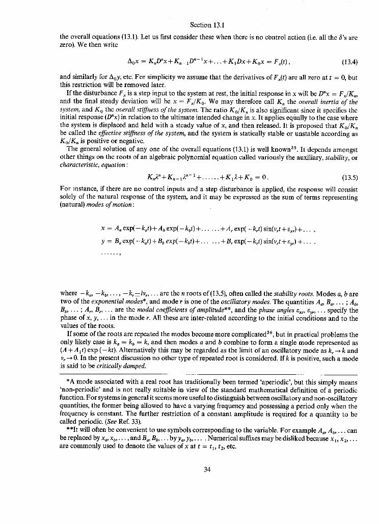
the overall equations (13.1). Let us first consider these when there is no ci~ntrol action (i.e. all the 6's are zero). We then write
Aox = KnDnx + Kn- 1 DR- 1X + . . . + K 1DX + KoX = Fx(t) , (13.4)
and" similarly for Aoy, etc. For simplicity we assume that the derivatives of Fx(t) are all zero at t = 0, but this restriction will be removed later.
If the disturbance F~ is a step input to the system at rest, the initial response in x will be Dnx = F,/Kn, and the final steady deviation will be x = Fx/K o. We may therefore call Kn the overall inertia of the system, and K o the overall stiffness of the system. The ratio Ko/K ~ is also significant since it specifies the initial response (D~x) in relation to the ultimate intended change in x. It applies equally to the case where the system is displaced and held with a steady value of x, and then released. It is proposed that Ko/K ~ be called the effective stiffness of the system, and the system is statically stable or unstable according as Ko/K~ is positive or negative.
The general solution of any one of the overall equations (13.1) is well known 35. It depends amongst other things on the roots of an algebraic polynomial equation called variously the auxiliary, stability, or characteristic, equation :
K,2 ~ + Kn_ 12 "- 1 + . . . . . . + K12 + Ko = 0. (13.5)
For instance, if there are no control inputs and a step disturbance is applied, the response will consist solely of the natural response of the system, and it may be expressed as the sum of terms representing (natural) modes of motion :
x = A, e x p ( - k.t) + A b e x p ( - kbt ) + . . . . . . + A~ e x p ( - k~t) sin(v,t + e~,) + . . . .
y = Ba e x p ( - k.t) + B b exp( - kbt) + . . . . . . + B~ e x p ( - k~t) sin(v~t + ey,) + . . . .
where - k , , - kb . . . . . - k , ± iv . . . . . are the n roots of (13.5), often called the stability roots. Modes a, b are two of the exponential modes*, and mode r is one of the oscillatory modes. The quantities A,, B~ . . . . ; Ab, Bb . . . . ; A,, B . . . . . are the modal coefficients of amplitude**, and the phase angles ex, er~ . . . . specify the phase of x, y . . . . in the mode r. All these are inter-related according to the initial conditions and to the values of the roots.
If some of the roots are repeated the modes become more complicated 36, but in practical problems the only likely case is k a = k b = k , and then modes a and b combine to form a single mode represented as (A + A it) exp ( - kt). Alternatively this may be regarded as the limit of an oscillatory mode as k~ --. k and v~ --* 0. In the present discussion no other type of repeated root is considered. If k is positive, such a mode is said to be critically damped.
*A mode associated with a real root has traditionally been termed 'aperiodic', but this simply means 'non-periodic' and is not really suitable in view of the standard mathematical definition of a periodic function. For systems in general it seems more useful to distinguish between oscillatory and non-oscillatory quantities, the former being allowed to have a varying frequency and possessing a period only when the frequency is constant. The further restriction of a constant amplitude is required for a quantity to be called periodic. (See Ref. 33).
**It will often be convenient to use symbols corresponding to the variable. For example A,, Ab . . . . can be replaced by xa, Xb, . . . , and B,, Bb . . . . by y,, Yb,- • • • Numerical suffixes may be disliked because x 1, x2 . . . . are commonly used to denote the values of x at t = tl, t2, etc.
34
Section 13.1
The exponential mode A exp(-kt) associatedwith a simple real linear factor (2 + k), is called a sub- sidence or a divergence according as k is positive or negative (stable or unstable mode). When there is a simple real quadratic factor (2z+ 2k2+co 2) ~i th co positive, it is convenient to write it also as ()~2 + 2Eco2 + co2~ where E is real. When Iel > 1 the quadratic factor has two distinct real factors correspond- ing to two separate exponential modes. When IEl -- I the factor is a perfect square (2+co) 2, k = ico , but there is just one corresponding mode as already mentioned, and such a mode is critically damped ifk = + co. When IEl < 1 the quadratic factor has two conjugate complex factors (2 + k + iv) and (2 + k - iv), which taken together correspond to an oscillatory mode which is stable or unstable according as k (and hence E) is positive or negative. A stable oscillation is variously described as damped, decaying, con- vergent, decreasing, etc., and an unstable one as negatively damped, growing, divergent, increasing, and so on. When its damping is zero (k = 0), an oscillatory mode has a constant amplitude, and it is said to be undamped or steady: in a panlinear system the frequency will naturally be constant.
The custom of using the words 'damped' and 'damping' when describing the response of a system would seem to clash with their application to terms in the original equations of motion. For a second- order equation there is no conflict, and this is why the dual usage has come about. It seems impracticable at present to abandon this usage*, but ambiguity can easily be removed by adding the word 'effective' when we refer to the response, although for measures of damping (see Section 13.2) this is unnecessary - it is unlikely that phrases like damping index or damping angle would be interpreted as referring to terms in the original equations.
It has been stated earlier that the effective damping of a mode, that is the stability of a mode, is directly connected with a root or roots of the stability equation. It is reasonable to define the quantity Kn- 1/Kn as the total effective damping of the system, since this is equal to the sum of the roots with signs reversed. It is thus equal to the sum of k,, kb , . . . , 2k . . . . . , which are the individual effective dampings of the modes. The system is stable provided that ka, kb . . . . . kr . . . . are all positive, whereas it is unstable if any of these are negative. The total effective damping is the amount available to be shared among the modes, and the' amount taken up by an oscillatory mode is 2kr, since the corresponding factors are (2 + kr + ivy) (2 + k r - ivy).
Oscillatory modes and pairs of exponential modes correspond to second-order equations, but a single exponential mode, which will always be present if the stability polynomial is of odd degree, corresponds to a first-order equation. In a mechanical system we have in general elements corresponding to inertia, damping, and stiffness, and a first-order equation cannot give a true representation of the dynamics. In some circumstances, however, a first-order equation may give an adequate approximation. Thus, when the stiffness is negligible, equation (13.2) reduces to
af~+bu = F , (13.6)
where u = ~, and when the inertia is negligible the equation becomes
bYc +cx = F. (13.7)
The effective damping of the system corresponding to (13.6) is b/a, and for (13.7) it is c/b. The general concepts of overall inertia and overall stiffness are still valid but the terms should be used with discretion. There is no difficulty when the equation is of order three, five, and so on.
Now consider the overall equations (13.1) when there is just one control action and no disturbance. We then have
A0x = hxS, 1 (13.8)
Aoy = Ay5,
and so on, which may also be written
x y A----~ = A---~ = ' " = A---~" (13.9)
*This matter is discussed in Ref. 33.
35

Section 13.1
It may be convenient to expand the denominators as
A~ = XID' + . . . + X1D + Xo, etc.,
and A o = K . D " + . . . + K 1 D + K o.
Equations like (13.9) have been introduced in Sections 12.1 and 12.2, and the polynomials A~,, At, . . . called complete response polynomials, in order that component parts could be called response polynomials.
When discussing steady-state relationships we need only'the constant coefficients, and we have
steady state g 0
The denominator has already been defined as the overall stiffness of the system, and the numerator is termed the trim power of the motivator 5 as regards the variable x. Further aspects of steady states and quasi-steady states of manoeuvring are discussed in Section 14.2.
If, on the other hand, we examine the initial response of the system (previously at rest with 5 zero) to a step change in 5, we have
t=0 K ,
This could be termed the 'coefficient of initial response', and (n - l ) would be the 'order of the initial response'. X t could be called the 'initial power' of the motivator as regards x.
It is customary also to relate the outputs x, y , . . . to an input such as 6 by means of transfer functions. It we write
x = Tx3 , y = Ty5 . . . . , (13.10)
then Tx(D), Tr(D), etc. are called transfer functions. Thus for panlinear systems and in our notation
Tx = A___~x Ao
X t D t + . . . X 1 D + X o
K , D ' + . . . K I D + K o
X 1 (D + bl) (D + b2) • • • (D 2 + 2bsD + c2) . . .
K , (D + ka) (D + kb) . . . (D 2 + 2krD + coff) . . . (13.11)
It is not implied by the example that numerical and alphabetical suffixes are always preferred for the numerator and denominator respectively. The American practice of writing a quadratic factor as (D2+ 2~oD + w2), which is the equivalent of our (D2+ 2EwD + co2), regardless of whether it belongs to a response polynomial or to the stability polynomial does not seem to have any advantage, as the coefficients bs, c, cannot in general be associated with physical characteristics like damping and frequency. However, for some purposes it is convenient to have a notation for the factors of (D 2 + 2b~D + c2), and these may be written as ( D + b s + ida) ( D + b , - ids).
36

Section 13.1
In particular, when for control purposes the input 8 is made to depend on a response variable x, the factors of the numerator of T~ may indicate limiting values of the stability roots. Thus, if 8 = 8o - Gx, where fi0 is an independent input and G a scaler parameter, we have
(Ao + GA~)x.= A~8o,
mx so that x = 80,
Ao + GA~,
and the stability polynomial for the closed loop is Ao + GA~. When G becomes very large, some of the stability roots then approach the roots of the numerator A~ of the open-loop transfer function.
It should be noted that if we take the (unilateral* or one-sided) Laplace transform of equations (13.8), and we write ~ for the transform of x, and 2 for the Laplace parameter, then
Ao(2) 2 = Ax(2) 3 + initial condition terms,
and therefore 2/3 is not always equal to T~(2). The latter is sometimes called the transform transfer function aT, although one should expect such a name to refer to ff/~. T(ico) may be called the harmonic transfer ratio (see Ref. 33), where o9 is the angular frequency ofa sinusoidal input.
The notation above can be extended to include a disturbance by writing
Aox = A~8 + Fxy,
where the disturbance Fx is expressed in terms of some variable ~), and F~ is a polynomial in D. We can also write
x = TxS+ T,V,
or x = Tx~8 + Tx~v,
where T~ is the control transfer function, and T~ is the disturbance transfer function. If it were necessary to include several control inputs 8,, 8b . . . . . and several disturbance variables 7a, VB, . . . . we would have to write something like
Ao x = AxS -b Ax8 d- . . . d- FAy A -b FBx y B -b . . . .
a b x = Tx8 . + Txbb +. . . + TAyA + T~ys + . . . .
13.2. Measures of Damping and Frequency. For both exponential and oscillatory modes the quantity A exp(-kt) is the amplitude at time t. The
contribution of a mode A exp( - kt) to the value ofx at t = 0 is just A, the initial amplitude, but the corres- ponding contribution of an oscillatory mode A exp( - kt) sin(vt + e) is A sin e, where 8 is the phase angle.
The quantity k is the damping index, and is a measure of the amplitude reduction per unit time. The quantity v is the angular frequency, and o~ is the undamped angular frequency. Each of these may sometimes be described as a natural . . . . . frequency to distinguish it from the frequency of an oscillatory input, which may be described as having a forcing frequency. It is often convenient to work in terms of the ratio (forcing frequency)/(natural frequency), and this may be called a relative frequency.
It is unfortunate that for many years the terms 'damping coefficient' and 'damping factor' have been
*See Brown a2
37

Section 13.2
used for both k and E, the latter defining damping as a fraction of critical damping*. Confusion should be avoided by the adoption of the term relative damping ratio for E. The shortened names relative damping or damping ratio would be admissible. The latter is already in widespread use in servomechanism literature, but it is suggested that the other shortened name is preferable. The relative damping ratio E is related to the quantities k, o~, v by the following relations:
E = k/og,
v = o ~ / 1 - E 2 .
When E < 1, the quantity ~ defined as sin- 1E is called the damping angle. It is related to the other measures of damping as follows :
= sin- l(k/o) = tan- 1(k/v).
The quantity P, defined by
P = 2n/v,
is the period of the oscillation.
For an oscillatory mode it can be convenient to express time in terms of the time angle (q0, or the number of cycles (C), where
q~ = vt ,
C = vt/27r,.
The corresponding analytical expressions for the mode are
A exp(- kt) sin(vt + e) = A exp( - xq0 sin(q~ + 5) = A exp( - AC) sin(2nC + 5)
= A exp( - xvt) sin(vt + e) = A exp(- At~P) sin(27rt/P + e),
where x is the angular damping index, and A the logarithmic decrement (cyclic damping index) or 'log dec'. These two measures of damping have been much used in the past, although x has not previously been given a proper name---it was sometimes referred to as the 'R-over-J ratio', where - R and J denoted the real and imaginary parts of complex roots. The three damping indices are related as follows:
k/v = x = A/2g = tan 6.
The ratio of the amplitude at any time t to its value at time ( t - 1) is called the persistence (G), and is equal to exp( - k). A mode is stable or unstable, the amplitude reducing or growing, according as the persistence is less or greater than unity. When the amplitude is constant the persistence is unity.
Corresponding angular and cyclic persistencies exist in principle, as for the damping index. However,
*Many writers have used the symbol D or ( to represent the fraction of critical damping. In aero- nautical work it would be acceptable to use one of these provided there were no clash with D denoting the operator d/dt or with ~ denoting rudder deflection or equivalent.
38

Section 13.2
an angular measure is not likely to be used, and for a cyclic measure it seems more useful to define a related quantity, the swing ratio* (F). This is the ratio of a peak excursion to the preceding one of opposite sign, and the oscillation is stable or unstable according as F is less or greater than unity. It should be noted that the cyclic persistence and swing ratio (or a sequence of swing ratios) will exist for any form of oscillatory response. The present section is essentially concerned with a simple linear mode, and in this case the swing ratio is equal to the persistence per half-cycle, which is given by F = exia(-½A). Even for a single linear mode the swing ratio cannot in general be interpreted as an overshoot factor, since the latter usually refers to thefirst overshoot and therefore depends on the initial conditions.
The time !t~) taken for the amplitude to diminish by a factor of e (2.718...) has often been called the time constant or damping time. The latter is not a good term because it might be interpreted as the time taken for the amplitude to decrease to some specified value, but the only objection to the former is that 'time constant' is also used extensively for specifying parameters of isolated elements with first-order lag. Thus an element with transfer function 1/(1 + ~D) is said to have a time constant of~.
It is proposed that t~ be called the time to one-over-e~ but the symbol T may be used instead, particularly when additional suffixes are required. It is suggested that this quantity should not be called a time constant unless it is clear that it refers to a mode of motion rather than an element of the dynamic system. When the latter is a first-order one, it does not matter which term or symbol is used. In general, however, the values of t~ for the various modes are complicated implicit functions of any z time constants of elements of the system.
Corresponding t o t~ there are angular and cyclic measures of damping: the number of radians to one-over-e (r,~) and cycles to one-over-e (C~). It is obvious that t_, = 1/k,.r~_ = l/x, C~_ = 1/A.
If a tangent is drawn to the curve exp(-kt) , then the intercept on the time axis is always equal to t~, as illustrated.
exp (-kt)
I _ t j . _ ~ L t j . d t
*In the past the term 'attenuation ratio per half-cycle' has sometimes been used. The term 'amplitude ratio' is not considered available as it is much used for other purposes. If angular and cyclic persistencies were defined, F and Fc would be appropriate symbols, and F~ would denote the swing ratio. The term persistence index seems reasonable for the quantity a = - k (see Ref. 33).
39

Section 13.2
In practice many people prefer to deal with amplitude changes of 1/2 rather than 1/e. This may be interpreted as a preference for writing 2-k~,t instead of exp( - kt), where
k kB = loge2'
and may be called the binary dampin9 index*. The time to half-amplitude (t~) is equal to 1/kn. The corresponding angular and cyclic quantities may be defined but the angular ones are not likely to
be used. We thus define the binary Io9 dec (An), and its reciprocal the number of cycles to half-amplitude (C~), where
A 1 A B - log~2 = C½"
Occasionally unstables modes may be described in terms of t t or C~, the time or number of cycles to double-amplitude.
Of the symbols discussed above, only a few are required when the time-vector method as'a9 is used for representing the contributions of an oscillatory mode in each equation of motion, and each kinematic equation, by a polygon of vectors. The undamped angular frequency (co) and the damping angle (6) are required for all response variables, and the relative phases of the latter are denoted by ~ with suitable suffixes as described below.
A quantity u = u~ exp(-kt) sin vt is represented as a line of length u~ at zero phase. Since
fi = coul exp( -- kt) cos(vt + 3)
"= O)U 1 exp( - kt) sin(vt + ½~z + 6),
fi will be represented by a line of length wul at phas e (½rc + 6). Similarly,
ti = cn2ul exp( - kt) sin(vt + rc + 26),
and
f ud t 1 = -- ul exp( - kt) sin(vt-½zc- 6), O)
*It is suggested in Ref. 20 that 'exp' can be given more generality, so that in our case we could write
exp(- kt) = exp2(- kBt).
' 40
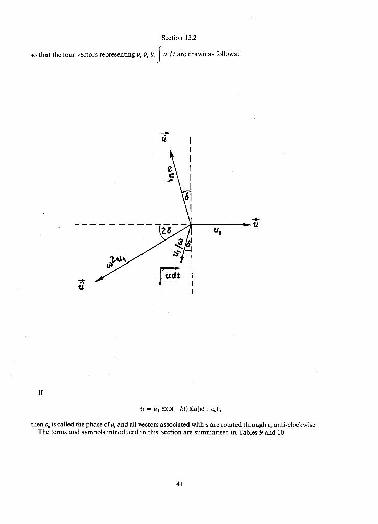
Section 13.2
so that the four vectors representing u, ~i,/i, f u d t are drawn follows a s
d
ti I
tg
t/1
If
u = ul e x p ( - kt) sin(vt + ~u),
then 5u is called the phase of u, and all vectors associated with u are rotated through su anti-clockwise. The terms and symbols introduced in this Section are summarised in Tables 9 and 10.
41

Section 13.2
T A B L E 9
Measures of Damping.
N a m e
Damping index
Angular damping index
Logarithmic decrement (cyclic damping index)
Relative damping ratio (relative damping,
or damping ratio)
Damping angle
Binary damping index
Binary log. dec.
Time to 1/e
Radians to 1/e
No. of cycles to 1/e
Time to half-amplitude
Radians to halgampli tude
No. of cycles to half-amplitude
Symbol
A
E (or ~)
kB
AB
t~ (or T)
r ! e
C~
t~
r½
C~
Definition
Ampli tude = A exp( - kt)
Ampli tude = A e x p ( - kvt):
therefore x = k/v = tan 6
Ampli tude = A exp( - At~P): therefore A = kP = 2nx
Ampli tude = A e x p ( - Eogt): therefore E = k/o9 = sin
= fraction of critical damping
= s in- 1E = t a n - 1 (k/v)
Ampli tude = A 2 - k~t :
k therefore kB -- - -
loge2
Ampli tude = A2-a'a/e:
A therefore A B -
1Oge2
t~r
1 C~
t~ = I/k
r ~ = 1/tc
c ~ = UA
r½ ~ q
C ~ -
loge2
k
loge2
1Oge2
A
42

Section 13.3
TABLE 9--continued
Measures of Damping
Name
Persistence
Persistence per cycle
Swing ratio
Symbol
G
Fc
F (or G)
Definition
Ratio of amplitude to its value one unit of time earlier
G = ex p ( -k ) = exp(cr)
Ratio of amplitude to its value one period earlier
Fc = exp( - A)
Ratio of a peak excursion to the preceding one of opposite sign
F = exp(-½A)
TABLE 10
Measures of Frequency.
Name
Angular frequency
Undamped angular frequency
(Cyclic) Frequency
Period
Undamped period
Symbol
09
Vc
P
Definition
No. ofradians per unit time
v = ( ~ 2 _ k2),
= CO C O S
Value of angular frequency if damping were zero
No. of cycles per unit time
vc = v/2n
P = 2n/v = 1/vc
Value of period if damping were zero
43

Section 13.3
13.3. A Discussion of the Merits of Various Measures of Damping. When the variations in stability of a complicated system are to be depicted as a parameter is altered, it is
usual to show the values of the damping index and the angular frequency of each mode of motion. Transi- tions of oscillatory modes into two exponential modes and vice-versa are then shown directly, transition points occurring when the frequency becomes zero and there are two coincident values of damping index.
When attention is confined to oscillatory modes, it is often preferable to represent the damping per cycle, and it is difficult to say which of the measures listed in Table 9 is the most convenient. Perhaps the most universally recognised quantity is the relative damping ratio, but it does suffer from the dis- advantage that much experience is necessary before one can correlate a given value of relative damping with the actual dynamic response of the system. Relative damping is a much more sensitive measure of changes in the response when the damping is low than when damping is more than half the critical value. Relative damping is a convenient algebraic paramcter, but it cannot be directly or simply derived from a record of the damped oscillation. The range of values of relative damping is very suitable, zero and unity corresponding to zero and critical damping respectively.
The above remarks are also relevant to the log dec (A) and the angular damping index (~). The latter can be more convenient algebraically than relative damping, but the scale of values is markedly non-linear and critical damping corresponds to n = oo.
It will be remembered that E = sin 6 and ~ = tan 6, so that E ~ K ~ 6 when the damping is low. The log dec is equal to 2n~ and therefore seems to be redundant except on historical grounds.
The time to half-amplitude and the cycles to half-amplitude have often been used, but there is a tendency now to use their reciprocals instead, that is the binary damping index and the binary log dec. It can be argued that the alleged convenience of the binary measures is superficial, since tables of exp(-x) are more readily available than tables of the function 2 -x. It is interesting that the binary log dec is approxi- mately equal to ten times the relative damping up to values of about E = 0.4 (As = 9.0647 tan 6, E = sin 6).
The persistence and the swing ratio are by definition directly related to the dynamic response presented in the form of a time-based record, and are unsuitable for algebraic work. One convenient way of estimating the persistence is to draw the 'envelope' of the record and then plot the logarithm of the amplitude (which is half the width of the envelope) against time. By taking two points on the resultant straight line (in practice the mean straight line) the persistence or the swing ratio can be read directly off the logarithmic amplitude scale. One point is taken at the intersection of one of the principal (multiple of 10) grid lines (see Fig. 6), and the other is taken unit time (or half a period) later. The log dec is almost as easy to deter- mine. Once the swing ratio has been found, the log dec can be calculated from the relation F = exp ( , ½A), either by consulting exponential tables, or taking logarithms, or by measurement of the scale factor used in plotting the amplitude. For this purpose, setting off a full period and first determining the persistence per cycle would be slightly more convenient, as F c = F 2 = exp(-A).
If the mean of the plotted points is very different from a straight line then the system dynamics is complex or markedly non-linear, and the question of what quantity is a valid measure of dynamic per- formance is raised. Even in a linear system it may be difficult to plot the amplitude of one particular mode when other modes are present, but a reasonable estimate may be made when the other modes are well damped and the mode being investigated is not well damped.
The damping angle and the relative damping are probably the most convenient of all the oscillation damping measures for use generally in the theoretical work, although it may be preferable to convert to other measures in order to interpret results. All the other measures, including relative damping, are elementary functions of the damping angle.
Corresponding numerical values of the oscillation damping measures are given in Fig. 7. An extended version of this diagram is given in Ref. 64, and covers a range of negative damping as well as positive.
14. Centres of Force and their Relation to Control Discriminants. 14.1. Centres of Pressure and Aerodynamic Centres.
It is sometimes convenient to pretend that some components of the aerodynamic moment are entirely due to forces acting at specific points, and these centres of force are traditionally called centres of pressure.
44

Section 14.1
This is a well-known technique which replaces the forces and some of the moments acting on a rigid object by an equivalent system of forces. Increments of the moments from datum values may likewise be assumed to be the result of incremental force components acting at points called aerodynamic centres : it is advantageous to generalise the term 'aerodynamic centre' which in the past has been restricted to a particular incremental force, namely the increment in lift due to an incremental change in angle of attack. The positions of the centres of pressure and the aerodynamic centres may vary with the flight conditions and the mass distribution of the aircraft.
Consider the definition of centres of pressure in terms of configuration body axes (see Section 4.1). For this purpose a force equal to X is usually assumed to act along the longitudinal axis, and the rolling moment L is not replaced by an equivalent force. The pitching moment M and the yawing moment N are then assumed to be produced by forces equal to Z, Y respectively actin~ at centres of pressure on the longitudinal axis, and their distances aft of the reference point (the origin) are given by
M N H = ~- , I - y , (14.1)
respectively. The reference point is usually taken to be in fore-and-aft alinement with the leading edge or other point on the second mean chord (see Section 16).
Centres of pressure and aerodynamic centres may be defined for parts of an aircraft as well as the whole : from now on, however, we shall consider the whole aircraft only.
The position of the centre of gravity may be specified by its coordinates xG, YG, zG, but it can be con- venient to write Ha for -xG. The out-of-balance moments on the aircraft are given by
L - mg(z~ma + y~n3),
Z H + mg(H~n3 + z J a ) ,
Y I - rag(Horn a + yol3),
where 13, ma, na are the direction cosines of the downward vertical relative to the configuration body axes. For a horizontal attitude la and ma are zero while n3 = 1, and if also y~, zG are zero the moments are equal to
L, Z H + m g H ~ , Y I ,
so that when Z = - m g the pitching moment becomes mg(H~-H). In a similar way an increment in the pitching moment (for example Mww')is assumed to be due to the
corresponding z-component of incremental force (Zww') acting at an aerodynamic centre on the longi- tudinal axis. The distances of such aerodynamic centres aft of the reference p o i n t - which might be called 'aerodynamic arms ' - -are given by
M. M,~ M. re=z- V, K°=z-
and so on. Similarly we may specify 'yaw' aerodynamic centres on the longitudinal axis in terms of aerodynamic arms such as
Nv Nr Jo : - - - ~ , J: = - y--~,
45

Section 14.1
aft of the reference point. Control discriminants 34, which are discussed in Section 14.2, can often be expressed conveniently in
terms of various aerodynamic arms. For example, a static trim margin for level flight can be defined as
K ~ = K ~ , - K u .
The distances H, H a, K . . . . . . I, J . . . . . are usually normalised in terms of the appropriate aerodynamic representative length, in which case small letters are used:
(h, ha, ku,...) = ~ (H, Ha, K . . . . . ),
(i,j . . . . ) = 1 (I, J . . . . ) • l z • .
Alternatively, ~,/~,,, j . . . . . may be used instead of h, k , , j . . . . . . so long as it is clear that the aero-normalised unit of length is 11 for longitudinal quantities and 12 for lateral.
When the terminology 'alpha and beta planes', 'alpha and beta incidence angles', is introduced (see Section 6.2), care should be taken, as the name 'alpha aerodynamic centre' could be misinterpreted (e might be used as an alternative variable to w).
14.2. Control Discriminants.
The ease with which an aircraft can be controlled through a particular motivator may be partly assessed by evaluating certain functions called control discriminants. It is assumed from the start that the aircraft can maintain any one of a range of steady flight conditions, each requiring its particular combination of motivator deflections. If we consider two steady states such that only one motivator has to be deflected by an increment 8' from its position in one state in order to maintain the other steady state, in which the other variables differ by increments x', y', . . . . and if also we can establish that
8' =f~x ' =frY' = . . . .
thenfx,fr , . . , are the control discriminants for the motivator 8 with respect to x, y . . . . . It is desirable that there should be no changes in sign of a discriminant when different pairs of steady
states are taken for one aircraft. Furthermore, it may be possible from flight experience to prescribe favoured ranges of values for some discriminants.
When each of the steady states is an equilibrium condition, and the increments in 8 and x, y . . . . are so small as to permit the Use of linearized equations, we may write, from equations (13.9) and (13.11),
x' y' 6
Xo Y0 Ko
since all the derivatives 2, 5/ . . . . . 3~, j) . . . . are zero• The control discriminants are therefore equal to Ko/Xo, Ko /Yo . . . . . and since these are related through K 0 to the classical concepts ~°,41,34 of static margin and static stability, they may be called static trim discriminants, although the term system trim discriminant might be preferred, particularly when systems other than aircraft are considered. There should be no confusion in merely calling them trim discriminants.
Similarly when one of the steady states is an equilibrium condition and the other consists of a manoeuvre (involving for example a steady angular velocity or a steady centripetal acceleration), the discriminants may be called manoeuvre discriminants by analogy with the classical term 'manoeuvre margin '42,43.
Many implications of this approach to the formulation of control criteria have yet to be explored, and it is premature to recommend a definite notation in this Report. It can be noted, however, that the quantity
46

Section 14.2
defined in Section 13.1 as the overall stiffness of the system is the same as the Ko involved in the static trim discriminant. Strictly a system can have only one Ko, but in the analysis of a manoeuvre the overall equations of motion can often be replaced by a simpler approximate set. The Ko for this set is called the manoeuvre stiffness. An alternative definition is often feasible based on approximate expressions for the transfer functions T~, Ty, etc.
For example, in the well-known theory of the manoeuvre margin it is assumed that the speed is constant during a pitching manoeuvre, and the longitudinal equations of motion for aerodynamic-body axes reduce to the approximate form
(l + z,~.) ~{" + zww' + (Zq - u~) q' + znq' = 0,
mvjv' + m~w' + (t' + mqq' + m,~/' = 0,
and the constant coefficient in the stability polynomial is then equal to (Uemw + z~mq- zqm~). This is quite different from the Ko given in Section 12.1 for the full equations, but it is often approximately equal to the coefficient Ka given there*.
A factor of Ko may be found to deserve special attention and definition. Thus, in the example just mentioned, if we divide by - Zw(ue + Zq/m)/Iy we obtain the factor
Mw K ? P I ~ m
Z~ mue+Zq'
which represents a length and can be interpreted as the distance between two points on the x-axis. It may be possible also to find significant factors of Xo, Yo . . . . .
Examples are given below for the static trim discriminant and manoeuvre discriminant corresponding to the flight conditions usually assumed for the definition of static and manoeuvre margins. The significant factors of the overall stiffness and of the manoeuvre stiffness are then lengths whose aero-normalised values are equal to, or nearly equal to, the classical static and manoeuvre margins. For example, the aero-normalised value of K,, (defined in the previous paragraph) is given by
if we assume that Zw ~ -CL~ a n d / l + ~q ~ p. In old notation the manoeuvre margin was equal to 21f mw m~'k c ~ ~ + ~ - ~ l ) ' but the new notation eliminates the factor 21/~.
It is proposed that in general the significant factor of the overall stiffness will be called the static trim margin or (system) trim margin and denoted by Ks, and that the significant factor of a particular manoeuvre stiffness will be called the manoeuvre maroin for that manoeuvre and denoted by Km.
The significant factors of the 'trim powers' X0, Yo . . . . are of the form (aM~ + bZ~ + cX~) and for most variables a will be made unity for a pitch motivator, b unity for a catanator, and c unity for a proaptor. The factors may be called 'trim power margins' for the motivator 6 and the variables x, y . . . . when belong- ing to the static trim discriminants, and 'manoeuvre power margins' when belonging to a manoeuvre discriminant. Power margins for x, y . . . . could be represented by X~, Y . . . . . or Xm, Y . . . . . as appropriate.
*In old notation the corresponding quantity (c0-Zw v) was approximately equal to the coefficient of 22 in the stability quartic. A quartic rather than a quintic was obtained because it was usual to assume that the atmosphere was uniform. It was also usual to neglect z~.
47

Section 14.2
It may be convenient also to have a name for the significant factor of the whole control discriminant, and 'control margin' is suggested. For example, the 'trim control margin' for the variable x would be equal to KJX~, and the 'manoeuvre control margin' equal to K,,/X,,.
The inverse of a control discriminant (i.e. Xo/Ko) gives the steady-state value of x produced by unit deflection of the motivator and may therefore be called the 'trim sensitivity' or 'manoeuvre sensitivity' as
appropriate. A significant factor would be called trim sensitivity margin ( ~ ) or manoeuvre sensitivity
margin' ( X - ~ ) •
It is suggested that the symbols for denoting control discriminant and sensitivity discriminant should be fix and x~ respectively since they can be interpreted as OS/~x and Ox/a6 respectively. Similarly the symbols for a control margin and sensitivity margin could be Kx and XK (Jx and Xj for lateral). When necessary a second suffix (s or m) could distinguish the cases of static trim and manoeuvre. Typical symbols arising in longitudinal examples would be flu, u~ Kv, UK (or t/.s, un . . . . . ) and t/q, q,, Ka, QK or t/q . . . . . ). Lateral examples would be {v, P¢, Je, P J (or {p,, . . . . ).
After the simple examples of Section 14.2.1 the general derivation of significant factors of Ko, Xo, Yo, . . . is discussed briefly in Section 14.2.2. It is concluded that specific definitions should not be laid down in this Report, although some indication of the notation can be given.
The control discriminants are functions of the position of the centre of gravity of the aircraft. It is sometimes possible to locate the points for which discriminants are zero, and such points would be called the neutral point or manoeuvre points, corresponding to the static trim discriminant or manoeuvre dis- discriminant respectively. If these points lie on the x-axis the distance of the pitch neutral point aft of the reference point is denoted by H,, and the distance of a pitch manoeuvre point by Hm. Similarly the position of the yaw neutral pointis specified by a distance I,, and yaw manoeuvre points by Ira. Normalised values are denoted by h,, hm, in, ira, or by/-2,,//m, i,, I,,, as is done for centres of pressure and aerodynamic centres Normalised values of the static trim margin and a manoeuvre margin are likewise denoted by k,, km or
When motivators are allowed to act freely without direct inputs from the pilot or control system actuators, the ideas developed above can be extended by treating the motivator deflection as one of the response variables x, y . . . . . For example, for a free elevator an additional system equation governing the elevator hinge moment is required, and tab deflection z may take the place of 6 in the analysis above. The additional suffixfcould be used for distinguishing static trim margins and the like in the motivator- free case, for example as in K~s. This is preferable to using K', in the Gates and Lyon style, since in the present notation K's could represent an increment in Ks.
14.2.1. Control discriminants for an aircraft in straight unbanked level flight.
(a} Static trim discriminants.
Consider two equilibrium flight conditions, one of which is straight and level, the other being a neigh- bouring condition with small perturbations u', w', 0, ~/' relative to the first, which is taken as a datum. It is assumed for simplicity that in both conditions the bank angle is zero and that perturbations in all other variables are zero. In addition body axes are chosen such that the centre of gravity lies on the x-axis.
In each condition the aerodynamic forces are in equilibrium with the gravitational force rag, and the resultant moment is zero. In the datum condition Xe and Me are zero, and Ze = - r ag : in the perturbed condition X' and (Ze + Z') must balance rag, and M' must be zero. In other words X' =mgO, and Z', M' are zero, since the components of gravity along the x and z-axes in the perturbed position are - gO and g respectively to first-order accuracy.
48

Section 14.2.1
Fig. 8 illustrates the incremental forces acting on the aircraft in its neighbouring equilibrium condition. The forces proportional to u', w', t/' are assumed to act along lines that intersect the x-axis at the points U, W, E which are at distances Ku, K~, K, from the origin. They can therefore be represented by the components X~u', Z,u' acting at U, and so on. For equilibrium,
X.u' + X~,w' + Xntl' = mgO ,
I i I Z.u + Z~,w + Zntl = O,
Muff + M~,w' + M d f = O,
where M., Mw, Mn may be replaced by K.Z. , KwZw, K,Z~, respectively. The algebraic solution of these equations is
where
A A~, Au Ao
A = rnoZ.Mw = m o ( Z . M ~ - Z~,M.)
= meZ.Zw(K~,- K.),
Aw = mgMuZ~ ,
A" = mgZwM n ,
Ao = M~XuZ~ + Z~MuXw + X~ZuM~, .
(14.2)
The static trim discriminants are A/Aw, A/A., A/A0, and they are also equal to
- Z w ( K w - K . ) Z.( - K. ) mg Z.Z ( - K . )
M , - K , Z n Mn - K~Z , A0
respectively. In order to relate these discriminants to the static margin we must take the expressions as given in
aero-normalised units. If then we say that (/(~ - / ( , ) is common to all three discriminants, and is further- more the only factor likely to change sign, we may claim that it is of particular significance and that it alone may form a basis for a criterion of static trim. This assumption is implied in the definition of static margin* by Gates and Lyon 4x, which however is not identical witll (/(~-/£~) even after allowing for differences in normalising divisors. They defined static margin in such a way that K, was in effect equal to
Z. 2Zw l (mw m. ' ]whenCR=CL. ZuZ'~(/£w-/£~) for in their notation K . = CL OCz/aa ~ \ z~ z u CLCL~ ]
This illustrates the arbitrary nature of the definition of a significant factor of the control discriminants, but nevertheless we can propose some definite notation. It must be possible to extract a factor which is a length, and this may serve as the static trim margin Ks although it would not in general be identical with the classical static margin. The latter was defined for a particular system with a prescribed set of equations and the control discriminants were therefore completely specified : this must be so once the equations are established. The usefulness of the quantity Ks will be much reduced unless it too has a unique definition for any particular system, but this can be achieved only by agreement. These remarks apply equally to the yaw static trim margin (J~), and to any manoeuvre margins that may be defined (Kin, Jm).
*The old symbol was K,.
49
Section 14.2.1
Returning to the derivation of a static trim margin, we consider now an alternative approach to the algebraic development. We may treat the problem as one of statics, and take moments about U and Win Fig. 8. We then have
(K~ - K.) Znt f = - (K~,- K,) Zww' ,
and (K, - Kw) Z , t f = ( K w - Ku) Zuu' ,
and hence
rf -- Zww' Z.u'
K w - K . M r - K.Z~ M ~ - K~Zn " (14.3)
The expression for 0 is a little more complicated and may be obtained either by taking moments about the point of intersection of the forces proportional to u' and w', or by substituting for u', w' in terms of t/' in the X-force equation. The static trim margin is given by
Ks = K w - K , .
The point W is approximately the same as the traditional aerodynamic centre and is identical with it when aerodynamic-body axes are used. If there are no compressibility or distortion effects and if the thrust line passes through the centre of gravity, the aerodynamic centre U is practically coincident with G. In this simple case K s is virtually equal to the distance of G from the neutral point, but this is not true in general. Complications in fact arise as soon as we take the datum condition to be non-level, quite apart from variations in the positions of aerodynamic centre and the centre of gravity. Expressions for static trim discriminants in the general case are given in Section 14.2.2.
(b) Pitching manoeuvre at constant speed.
Consider an equilibrium flight condition which is straight and level, and a neighbouring steady state in which a constant rate of pitch q ( = q') is maintained by an elevator deflection r/' relative to the datum value r/e of equilibrium. Corresponding perturbations in the other longitudinal variables will in general exist (u', w', 0) and a proaptor deflection v' may be required. It is assumed that the aircraft is unbanked in each condition and that all perturbations take place in the longitudinal (vertical) plane.
Manoeuvre discriminants cannot be defined unless approximating assumptions are made, and it is usual to postulate that
(i) linearized equations for small perturbations are valid,
(ii) terms in 0 (i.e. gravitational) can be neglected.
This leads to three equations in the five variables q', w', u', q', v', and if we adopt for simplicity aerodynamic- body axes with the x-axis passing through the centre of gravity the equations are
X,Tr f+Xww'+X.u '+Xqq+Xvv ' = 0, 1
Z,~tf + Z,,w' + Z,,u' + (Zq + mue) q + Zvv' = 0,
p / / t M~l + Mww + M,,u + (Mq + mueHa) q + M~v = O.
(14.4)
Some constraint must be imposed before these equations can be solved for the ratios rf/w', etc. The classical manoeuvre margin was based on the constraint u' = 0, and the small effects due to Z~ and My were ignored. Simple manoeuvre discriminants are then obtained, and a significant length along the x-axis
50

Section 14.2.1
extracted, but this is not possible if other constraints such as v' = 0 are assumed. The general problem is discussed in Section 14.2.2, and here we restrict ourselves to the classical assumptions already mentioned.
If we wish to reduce the problem to one of statics, we assume that forces X~w', Zww' act at the aero- dynamic centre W, and so on (Fig. 9). It is also convenient to define a centre of force C at which the resultant of the aerodynamic force Zqq and the centrifugal force mueq is assumed to act. We define
, Mq Mq +mueH o gq = --~r - Z 4 Zq + mu e
(14.5)
Mq and Zq are normally negative, and C is therefore forward of G. Taking moments about C and W, we have
* t (K~ - Kq) Z,t l - (K~ - * ' = Kq) Zww ,
(K~- Kw) Z,q' = (Kw - Kq) Zqq ,
and hence
rf - Zww' Z qq K~ - Kq M~ - KqZ. M. - K~Z.
(14.6)
This provides a basis for a manoeuvre margin K m equal to (K w - Kq), and, if we allow for the difference in normalising divisors, /(m is in fact exactly equivalent to the classical expression, provided that Zw is replaced by its approximate value CL~, Zq is neglected in the denominator 0f(14.5), and the origin is at G.
14.2.2. General interpretation of control discriminants. When the aircraft is taken to be completely rigid and we consider purely longitudinal motion, there are just the three equations in X, Z, M and in seeking ratios ~f/u', etc. we must restrict the number of variables to four. Let us assume that the four increments are unspecified to begin with, and denoted merely by xl, x2, xa, x4. The incremental forces proportional to xl, x2, xa, x4 are assumed to act at points P1, P2, P3, P4 which are at distances K1,. . . from the origin 0 (Fig. 10). The components along body axes are X~x~, Z~xa . . . . and the moments are M l x l = K1Zlx l , and so on, where X1, M1 . . . . stand for oX/Oxl, aM/Oxl, etc.
It is convenient to take Z~xi as the variables in order that the equations can be written as
I C1 C 2 C 3 C4
1 1 1 1
K1 K2 K~ , K 4
I Z l x l I = 0, Z2X 2
Z3x3
Z4x4
(14.7)
that is C1ZlXl+C2Z2x2+C3Z3x3-l..C4Z4x 4 = 0 , etc. where C i = cot el = Xi/Zi. The solution of equations (14.7) is
Zlx___~l = - Z 2 x ~ _ Z a x ~ _ - Z4x~
A1 A2 A3 A4 ' (14.8)
where A1 = (K2 - K3) C4 + (Ka - K4) C2 + (K4 - K2) Ca
= K 2 3 C 4 -b K 3 4 C 2 q- K 4 2 C 3
= -- K2 Ca4 -~ Ka C42 - K4C2a ,
51

Section 14.2.2
if we write K23 = K 2 - K a, C23 = C 2 - C 3 , etc.
Similarly A 2 = Ka4Ci + KglC3 + K 1 3 C 4
= - K3C4.1 - KgC13 - K 1 C a 4 ,
A 3 = K 4 1 C 2 d - K 1 2 C 4 + K 2 4 C 1
= - K4CI 2 - - K 1 C 2 4 - K2C41 ,
A4 = K 1 2 C 3 + K23C1 + K 3 1 C 2
= - K 1 C 2 3 - - K2 Ca I - K a C i 2 .
The A~ are lengths but a direct geometrical interpretation may not be illuminating. It is sometimes possible to divide equations (14.8) by a factor (say ,~), and at the same time to rearrange them to give
X 1 - - Z2X2 Z a x 3 - Z4xd-
2A, 2A2Z, 2A3ZI 2A4Z,
i.e. x_& = - Z'zxz _ Z'3x___~3 = __- Z'4 x 4 (14.9) A4Zi A3Z1 A2Z1 A'l . . . . . . .
where A'I is a more suitable length than A1, and some of the other denominators in (14.9) can be expressed
as
A'2Z'I = M l + a z Z l +b2X1
= M1 +a'2Z'~ +b'zX'~, (14.10)
and so on. If x~ is identified with a motivator deflection t/' the denominators defined as in (14.10) are modified M, type derivatives and can be called trim power margins or manoeuvre power margins as mentioned earlier.
One way of finding a factor 2 is to choose the line of action of one of the forces R~, say R4, as a base for centres of force and aerodynamic centres. Suppose the lines of action of R1, R 2, R 3 meet the R4 line at Q1, Q2, Q3 and that P4Qi, P4Q2, P4Q3 are equal to K~4, K' ' 24, Ka4. As illustrated at Q~ we can assume incremental forces X'~xt, Z'lXl to act at these points, and we can impose the condition that the moments
7, K ' and so on. It is found that about P4 are unchanged, so that Z1K14 = ~ t4,
K14 = K'14C41 sin e4,
Z'l = Z iC4i sin e4
= Z~ c o s e 4 - X 1 sin e4,
X'~ = X~ cos e4+Z~ sin e4, etc.,
and equations (14.9) are then valid if we choose
A'l A1 , , = - K 2 4 - K a 4 , (14.11) C42C43 sin e4
52

Section 14.2.2
ZI(K3C4-K4Ca)-X1Ka4 } A2Z-------!I=MI~ A~Zi = C43 C43
AsZ1 MI+Zl(K2C4-K4C2)-X1K24 A;Z~ = C42 C42
(14.12)
The length A~ has thus been given a direct geometrical meaning, namely the distance Q2Q3, and the quantities A'2Z't have the desired form. With this particular transformation based on the force R4, it is not surprising that the expression for x4 is dissimilar to the others and that Z',/A'4Z'~ is an indeterminate form. The transformed solution is in fact given by
x~ -Z'2x2 Z;x3
K' K' 2 4 - - 34 A'2Z'I A'aZ'I
R4 sin(e3 - e4) sin(e2 - e4) -Z tA 4 sin ea sine2
(14.13)
where A'2Z't and A'aZ'~ are given by (14.12) or alternatively by
and
[ K, ] A'2Z't = M1-Z'I K'a4q C41 sine4
E "+/sm l A'3ZI = M t - Z i Ki e4
-A4Z 1 = M1C23+ZI(K2Ca-KaC2)-XIK23.
(14.14)
Thec°ttermssuchasC2'C23can°fc°ursebereplacedbyX2/Z2'( X2Z2 X 3 ) ' a n d s ° ° n ' Z 3
To illustrate this technique consider the general trimmed equilibrium condition where the datum attitude is ®e" In the neighbouring condition illustrated in Fig. 11, the incremental force due to gravity is mgO along the line GQ1, and we shall take this to be the R 4 line, the origin being chosen to be at the centre of gravity. If we define GU, GQ3 to be K~, K °, etc. and define derivatives
X ° = Xu cos ®e + Zu sin ®e,
Z ° = Zu cos @e- X~ sin 0~,
and so on, the equivalent of equations (14.13) becomes
~ l 0 p - - Zww Zu°u '
0 0 ~ 0 0 ~ 0 0 K~, - K. M~ - K~ Z n M~ - KwZ~
mgO MnC +Zn(K C K C )-XnK w i t 19 u - - It Pd w u
(14.15)
3

= KwZw, where as before Mw = K~Z~ o o
XW Cwm
Zw
Cwu = C w - C, ,
K~. = K ~ - K., etc.
If we had drawn the diagram to show the datum state, the line GQ1 would have been horizontal, the derivatives X °, etc. would have been those along horizontal and vertical directions*, and the static trim margin can be interpreted as the distance between w' and u' aerodynamic centres fixed on the horizontal line through the centre of gravity.
The analogous treatment of the manoeuvre case is not so straightforward, and will not be discussed here.
Acknowledgements.
This Report includes many ideas arising out of earlier deliberations of an R.A.E. Panel (C. H. E. Warren, A. K. Weaver, S. Neumark, H. R. Hopkin) and out of more recent discussions with H. H. B. M. Thomas and others.
*It is important to distinguish between X ° and X°~, (see Section 20), but the latter is not required here.
54
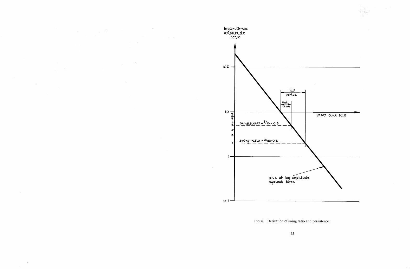
logo..rLt'hmLc o.'rE pl LI: u.cL e.
5CO.IE
I 0 0
hel~ F~.t Cod.
I0
7" 6- 5-
4-
3"
m
O ' l - -
~ p t ~ - s L s l : ~ = S/=o = 0,5
_sw__L~ ~ L o = ~/,o= o,~
plok oF Io~ O.mpICl:ud.e. ~eL'n.sl; l:¢.me.
v
FIG. 6. Derivation of swing ratio and persistence.
55

Swing r a t i O
F
0
Damp.ing angle
90 ° - - 5 0 0
- - - 4 0 0
0-I -
-_---:50 °
0 " 2 - - - Z5 o
0-3--~_- ZO O
o-4--- - _ _ 1 5 o
0-5- -
__ I0 ° o.6--_
0.7---~_
_ _ 5 0
0-8--
0 - 9 - -
I -0 0
Relative damping
E
!'0 0-8--- 0.7-
0"6-
0"5- - -
I
0 "3-~_
0"25--
0 " 2 0 - -
o-15-~
0 " 1 0 - -
0-05
0
FIG. 7. Nomogram of equivalent measures of damping.
Angular pro. p i n g l n a e x
K
oO - - 1 " 5 - - i "0 - - 0 - 9 - - 0 " g
0"'/
- 0 " 6
0"5
0"4
- - 0 -3
0-25
0-20
Zo.is
0"10
0"05
__
Critical damping
A " h o r i z o n t a l ' I {n¢
. i n d i c a t e s e q u i v a l e n t v a l u e s
Zero damping
log dec
A
Binary log dec
- - O O OO
7 10 6
5 7
6 4 - -
5
2 - 5 - - -
- - 3 2 - 0 - - -
- 2-5
I - 5 - --2-0
- - I - 5 I - 0 _
+--
- - i ' 0
0 - 5 - - -
0-5
0 0
A B
Cycles h a l f
t o ampl.
C ~/z 0 ,
0 - 1 - -
Swing ratio
I- 0
m
"--o.=
0 . 2 - - . 0"2
0.32_-0"3
:--0"4 0 " 4 - - -
0"5 Z 0-5
0.6--
0-7 - - 0-6
0 - 8 - -
0.9 - I ' 0 - - - - 0 - 7 h i - - - I - 2 - - - I -3 - - -~ 1 " 4 - - - I - 6 - - _ 0-8 l -B- - 2 - 0 - - -
3 - - - o . 9
7 - - - IO---- ZO-- z oo I'0
56

o.e~-od.~no.mLc cen.~r-e~ ~ o
.... ... o ~ _ ~ , ~ , o ~ ,
'~:~'~' K,, ~ '
FIG. 8. Equilibrium of incremental forces (level datum).
FIG. 9, Incremental forces in a steady pitching manoeuvre,
57

Z t 4 "1"4
R t
K t
R2
K~
R,
FIG. 10. Equilibrium of four incremental forces.
FIG. 11. Equilibrium of incremental forces. (Non-level datum).
Printed in Wales for Her Majesty's Stationery Office by Aliens Printers (Wales) Limited Dd. 135646 K 5
58

R. & Mo No. 3562, Part 3
(~ Crown copyright 1970
Published by HER MAJESTY'S STATIONERY OFFICE
To be purchased from 49 High Holborn. London w.c.1
13a Castle Street, Edinburgh EH2 3AR 109 St. Mary Street, Cardiff cF1 Ijw
Brazennose Street, Manchester i 60 8AS 50 Fairfax Street, Bristol Bsl 3DE 258 Broad Street, Birmingham 1
7 Linenhall Street, Belfast BT2 8A7 or through any bookseller
R. & M. No. 3562, Part 3
SBN l 1 470228 4