a scheduling scheme in the cloud computing environment

ARTICLE IN PRESS

JID: INS [m3Gsc; November 1, 2019;14:9 ]

Information Sciences xxx (xxxx) xxx

Contents lists available at ScienceDirect

Information Sciences

journal homepage: www.elsevier.com/locate/ins

A scheduling scheme in the cloud computing environment

using deep Q -learning

Zhao Tong

a , ∗, Hongjian Chen

a , Xiaomei Deng

a , Kenli Li b , Keqin Li b , c

a College of Information Science and Engineering, Hunan Normal University, Changsha, 410012, China b College of Information Science and Engineering, Hunan University, and National Supercomputing Center in Changsha, Changsha,

410082, China c Department of Computer Science, State University of New York, New Paltz, New York, 12561, USA

a r t i c l e i n f o

Article history:

Received 7 June 2018

Revised 29 July 2019

Accepted 17 October 2019

Available online xxx

Keywords:

Cloud computing

Deep Q -learning algorithm

Directed acyclic graph

Task scheduling

WorkflowSim

a b s t r a c t

Task scheduling, which plays a vital role in cloud computing, is a critical factor that de-

termines the performance of cloud computing. From the booming economy of information

processing to the increasing need of quality of service (QoS) in the business of networking,

the dynamic task-scheduling problem has attracted worldwide attention. Due to its com-

plexity, task scheduling has been defined and classified as an NP-hard problem. Addition-

ally, most dynamic online task scheduling often manages tasks in a complex environment,

which makes it even more challenging to balance and satisfy the benefits of each aspect of

cloud computing. In this paper, we propose a novel artificial intelligence algorithm, called

deep Q -learning task scheduling (DQTS), that combines the advantages of the Q -learning

algorithm and a deep neural network. This new approach is aimed at solving the prob-

lem of handling directed acyclic graph (DAG) tasks in a cloud computing environment. The

essential idea of our approach uses the popular deep Q -learning (DQL) method in task

scheduling, where fundamental model learning is primarily inspired by DQL. Based on de-

velopments in WorkflowSim, experiments are conducted that comparatively consider the

variance of makespan and load balance in task scheduling. Both simulation and real-life

experiments are conducted to verify the efficiency of optimization and learning abilities in

DQTS. The result shows that when compared with several standard algorithms precoded

in WorkflowSim, DQTS has advantages regarding learning ability, containment, and scala-

bility. In this paper, we have successfully developed a new method for task scheduling in

cloud computing.

© 2019 Elsevier Inc. All rights reserved.

1. Introduction

Currently, scientific computing and e-commerce applications are coherent models with interrelated tasks that can be

described as models of workflow, and these dependent tasks can be decomposed into tens of thousands of small tasks,

depending on the application complexity. The workflow model is extensively applied to represent these applications via DAG,

in which its nodes represent tasks, and its directed edges represent dependencies as in precedence task relations [1] . These

large-scale workflow applications are deployed in the cloud computing environment rather than the traditional distribution

∗ Corresponding author.

E-mail address: [email protected] (Z. Tong).

https://doi.org/10.1016/j.ins.2019.10.035

0020-0255/© 2019 Elsevier Inc. All rights reserved.

Please cite this article as: Z. Tong, H. Chen and X. Deng et al., A scheduling scheme in the cloud computing environment

using deep Q-learning, Information Sciences, https://doi.org/10.1016/j.ins.2019.10.035


http://www.ScienceDirect.com

http://www.elsevier.com/locate/ins

mailto:[email protected]



2 Z. Tong, H. Chen and X. Deng et al. / Information Sciences xxx (xxxx) xxx

ARTICLE IN PRESS


system for a shorter task execution time. None of the current approaches or methods can singly fulfill task scheduling

due to its unique characteristics. Specifically, guided random search-based scheduling is a new computing paradigm with

robust capability for solving task-scheduling problems. However, such stochastic algorithms have drawbacks, such as creating

considerable time complexity and contending with the dynamic cloud environment and its miscellaneous complications that

have made it even more unadaptable.

With the development of artificial intelligence, researchers now use stochastic algorithms such as the genetic algorithm

(GA) [2] to optimize the weight and threshold of back-propagation (BP) neural networks. This approach is used to solve the

problem of performing a task under multiplex conditions with unknown properties, where an agent is particularly needed.

Nevertheless, it is difficult to train a BP neural network without an obtainable training set from a complex environment

with indeterminable factors. Obviously, an agent is a correct action performed by an intelligent object trying to complete

a task. The action of an object in any given environment can be described as the process of the model’s decision making,

called Markov decision processes (MDPs) [3] .

The indeterminate nature of the cloud computing environment poses challenges to finding a proper algorithm for the

solution because of the typical phenomenon of randomness that accompanies task execution time. Although objective func-

tion is explicit to an equation or a value, the computing resource is dynamic, and feedback regarding the action of an object

in the scheduler is uncertain. In other words, a stochastic algorithm can hardly solve this random state process due to the

unclear objective function. Reinforcement learning methods, such as Q -learning [4] , are more reliable because a discounted

future reward is obtained when transiting from one state to another. Based on the foundation of MDP theory, Q -learning

is a useful and meaningful method for solving problems of agent actions under different complicated conditions. However,

in Q -learning, as the number of object states increases, the table matrix of the state action set in Q -learning becomes too

large to store and perform the search. With widely used BP neural networks, this problem is solved with a more concise

and accurate table matrix, and this approach is applied by more researchers.

Recently, the environment in dynamic decision-making is becoming more and more complex for a large number of al-

ternatives, high time constraints and uncertainty decision. However, the simple task that consisted of decision process is

simple that with less properties and constraints. Simple tasks can also have dynamic complexity in the continuous time

strategy. RL algorithms advance modeling in a continuous dynamic and complexity environment, using RL algorithms for

dynamic decision making has become a new research direction [5] . RL is highly effective in dynamic dispatch optimization

problems [6] . Recent works present deep reinforcement learning as a framework to model the complex interactions and

cooperation in dynamic decision-making environments. Yang et al. [7,8] have done multi researches on DRL in decision-

making with the subject of Deep Multi-agent Reinforcement Learning (RDMRL). Wang et al. [9] applied deep reinforcement

learning to dynamic resource scheduling for network slicing, and dynamically adjust the resources allocated to each slice

through interaction with network environment. Grag et al. [10] proposed a traffic light control strategy based on the deep

reinforcement learning method to solve the congestion problem near the road intersections. Google’s DeepMind applied a

deep Q -network (DQN) [11] to train agents in a convolutional neural network (CNN) that acquired only image pixels of

games and successfully surpassed human-level skill. This method has also provided new approaches to autonomous driving,

artificial intelligence, big data analysis, and so on. Motivated by this method, we implement the deep Q -learning method to

complete jobs in task scheduling accurately and to verify the adaptability in a more complex environment, such as in the

elastic cloud environment and online task scheduling.

In this paper, we propose a novel artificial intelligent workflow-scheduling algorithm, called deep Q -learning task

scheduling (DQTS). This new approach combines a back-propagation network and Q -learning algorithm for their respec-

tive advantages in obtaining less makespan of workflow in the cloud computing environment and achieving the best load

balance in each computing node. The main contribution of this paper is as follows:

• We propose a training algorithm along with a training set defined in a dynamic online task-scheduling problem and

illustrate the structure of the DQTS algorithm in the cloud computing environment, defining the cloud model, task

model, and scheduling architecture.

• We design the program framework, forward the model using cross-platform implementation, optimize hyperparame-

ters within programs and implement the DQTS algorithm for dependent workflow task scheduling.

• We implement the entropy weight method to the principle design of a bi-objective optimization problem (including

makespan and load balance) and apply the novel DQTS algorithm to produce a high-quality solution in dynamic cloud

computing.

• We assess the algorithm performance using WorkflowSim and compare it with different workflow benchmarks (in-

cluding CyberShake_20 0 0, Inspiral_20 0 0, Montage_20 0 0 and Sipht_20 0 0). The results show that our algorithm im-

proves the performance both in makespan and load balance.

The rest of this paper is organized as follows. Section 2 presents the related work on scheduling algorithms in the

cloud computing environment. Section 3 describes the cloud computing environment, task model, and scheduling structure.

Section 4 explains the main content of DQTS, with the theory and design principle. Section 5 compares the performance

of the proposed algorithm with existing classic algorithms and analyzes the experimental results. Section 6 concludes the

paper and introduces directions for future work.




Z. Tong, H. Chen and X. Deng et al. / Information Sciences xxx (xxxx) xxx 3

ARTICLE IN PRESS


2. Related work

Task scheduling is a well-known NP-hard problem since an efficient polynomial-time algorithm does not exist; conse-

quently, a considerable number of artificial intelligence algorithms have been proposed to obtain a suboptimal solution.

Furthermore, these algorithms commonly focus on minimizing the execution time, called makespan. There are three typ-

ical scheduling algorithms that have been proposed: the list-scheduling algorithm, clustering-scheduling algorithm, and

duplication-scheduling algorithm. Among them, the list-scheduling algorithm is the most widely used heuristic algorithm,

and the classic list-based heuristics-scheduling algorithm implements features that include heterogeneous earliest finish

time (HEFT) [12] , stochastic dynamic-level scheduling (SDLS) [13] , predicted earliest finish time (PEFT) [14] , and improved

predicted earliest finish time (IPEFT) [15] . Commonly, these algorithms accomplish scheduling in two steps: first, construct-

ing a sequence of tasks by assigned task priorities, and second, sequentially allocating each task from the sequence to

computing nodes that allow for the earliest start time. Clustering heuristics algorithms map all tasks with an indefinite

quantity to different clusters [16] . In contrast to list-scheduling heuristics, clustering heuristics algorithms require a sec-

ond phase to schedule task clusters to the processors. Under these conditions, only a sufficient number of processors can

result in an advantage, which is impractical in practice. Typical clustering heuristics algorithms include techniques of domi-

nant sequence clustering (DSC) [17] , task duplication-based scheduling (TDS) [18] , and heterogeneous selection value (HSV)

[19] . The duplication-scheduling algorithm can efficiently reduce the makespan of scheduling DAG tasks when the commu-

nication cost is significant, that is, the duplication method can effectively reduce or avoid interprocessor communication.

Many algorithms have been proposed to incorporate this technique into scheduling [20,21] . Bozdag et al. [22] addressed

the problem of scheduling that requires a prohibitively large number of processors, proposing a combination of the SDS

and SC algorithms to obtain a two-stage scheduling algorithm that produces schedules with high quality and low processor

requirements. However, for computation-intensive tasks, the performance of these algorithms is not significant. In recent

years, most researchers are studying grids, clusters and other typical heterogeneously distributed computing environments,

and task scheduling is performed for only a fixed number of resources. In contrast to the cloud computing environment,

cloud service providers often offer a better and scalable resource, and the tasks accepted are also arranged differently ac-

cording to their variance and type.

In the cloud computing environment, some related work on workflow scheduling strategies research is presented. For

instance, Teylo et al. [23] proposed a new workflow representation, in which nodes of the workflow graph represent ei-

ther tasks or data files, the edges of the workflow graph represent their relationship, and this workflow defines the task-

scheduling and data assignment problem as a new model. It is worth noting that they also formulated this problem as an

integer-programming problem. Wang et al. [24] presented a solution, the objective of which is to minimize the data transfer

of workflows allocated in multiple data centers. In this way, the purpose of reducing communication between nodes can

be achieved. To this end, his work defined the initial data locality by using the k -means clustering algorithm. Arabnejad

and Barbosa [25] proposed the multi-QoS profit-aware scheduling algorithm and achieved good adaptability by studying the

scalability of the algorithm with different types of workflows and infrastructures. The experimental results proved that their

strategies improved cloud provider revenue significantly and obtained comparably successful rates of completed jobs. Zhao

and Sakellariou [26] proposed the merging of multiple workflow applications into a single DAG workflow, and by using this

method, the job can be finished through any traditional DAG scheduling algorithms to minimize the total makespan and

achieve overall fairness. This approach is formulated and resolved based on issues of competition in resources with multiple

other DAGs. Kanemitsu et al. [27] proposed a prior node-selection algorithm (LBCNS) to select a subset of given nodes to

minimize the schedule length while fairly scheduling each job. The experimental results show that their algorithms have

the best fairness for scheduling multiple workflow jobs, while the priority-based approach achieves the minimum schedule

length with the highest efficiency for single- or multiple-workflow jobs. Chen et al. [28] proposed a scheduling algorithm

incorporating both event-driven and periodic rolling strategies for dynamic workflow scheduling. The experimental results

show that their proposed algorithm performs better than classic algorithms. Zhang et al. [29] proposed a novel reliability

maximization with energy constraint (RMEC) algorithm that incorporates three important phases, including task priority

establishment, frequency selection, and processor assignment, and the RMEC algorithm can effectively balance the tradeoff

between high reliability and energy consumption. Based on both randomly generated task graphs and the graphs of some

real-world applications, the result shows that RMEC surpasses the existing algorithms. Wei et al. [30] proposed an intel-

ligent QoS-aware job-scheduling framework for application providers, which learns to make appropriate online job-to-VM

decisions for continuous job requests directly from its experiences without any prior knowledge. The experiment uses the

real-world NASA workload traces, and the results show that the algorithm reduced the average job response time to 40.4

compared with the best baseline for NASA traces. Zhang et al. [31] proposed an energy efficient scheduling scheme based

on deep Q-learning model for periodic tasks in real-time systems (DQL-EES). The especial feature is the paper combining a

stacked auto-encoder in the deep q -learning model to replace the Q -function for learning the Q-value of each DVFS technol-

ogy for any system state.

Jiang et al. [32] proposed a corresponding algorithm that cooperates with a dynamic-voltage and frequency-scaling

(DVFS) technique to address the above concern and evaluated the algorithm in terms of randomly generated DAGs, real-

application DAGs and their hybrids under DVFS-enabled HCS. However, these scenarios, in general, are designed for a single

application that is not suitable for a dynamic cloud environment, where a large number of workflows will be submitted

from time to time. In addition, these complex environments have made task scheduling a difficult problem.





ARTICLE IN PRESS


Fig. 1. Model of task scheduling in cloud computing.

To the best of the authors’ knowledge, the approach proposed in this article is the first to use a deep Q -learning algorithm

to solve the workflow problem. In this way, we can consider both problems together by proposing a model as well as an

algorithm to minimize the makespan and find the best load balance of workflows in cloud environments. Our approach

takes into account different process capacities of the computing node, task execution time and data transfer time in these

cloud computing environments. The following section formulates the problems that are considered in this article.

3. System architecture and problem description

In this section, we first define the task model and model of cloud computing corresponding to the task-scheduling

scheme. Second, we propose the deep Q -learning scheduling architecture for the cloud environment and explain approaches

to obtain the training set for this model, the architecture of DQTS in WorkflowSim, and the neural network structure used

in this paper. Accordingly, we formulate the task-scheduling problem.

3.1. Cloud computing model

In cloud computing, tasks submitted by a user are allocated to cloud nodes based on the scheduling strategy. Therefore, a

proper selection of the scheduling strategy is vital for an optimal task completion time. Fig. 1 illustrates the model of online

dynamic task scheduling for a typical cloud computing scenario, in which users can submit their tasks at any time. In this

case, a task dynamically arrives at the task queue after user submission. The data center broker, depending on different

requirements such as makespan, load balance, economic principle, etc., selects the best scheduling strategy to allocate the

task to the computing nodes. In this paper, tasks are dynamically submitted to the scheduler by users, and the number of

tasks and types is unknown before they arrive at the task queue. We aim for the optimal distribution strategy to the cloud

nodes. Meanwhile, it is assumed that the tasks submitted to the scheduler are nonpreemptive. The computing nodes are

heterogeneous and scalable, but the bandwidth is the same.

3.2. Task model

The task model can be divided into the dependent task and independent task. Moreover, an independent task model has

the relationship of tasks such that they are independent and do not require any communication. Therefore, to achieve a

faster scheduling target, tasks can be preempted. Additionally, this kind of task scheduling is easy to implement. Generally,

dependent task scheduling models are composed of a set of dependent tasks and an interconnected processor. The depen-

dency of data and order of execution can be represented by a DAG. Therefore, the DAG scheduling model can be defined as

a quaternion:

G = (T , E, C, W ) (1)





ARTICLE IN PRESS


Table 1

Commonly used terms in DAG scheduling.

Notation Definition

t i task node

w i entropy weight

n total number of virtual machines

m i current task-processing time of each virtual machine

l i accumulated processing time of each virtual machine

Pred ( t i ) the predecessor set of node t i Succ ( t i ) the successor set of node t i IL ( t i ) the level of node t i P k no. k processor

ST ( t i : p k ) the start time of task t i on processor p k

FT ( t i : p k ) the completion time of task t i on processor p k

EFT ( t i ) the earliest completion time of the task

where T = { t i | i = 1 , 2 , . . . , n } , denotes the collection of n task nodes. | T | = n corresponds to the vertices in the DAG. Each

node in the DAG represents a task of a parallel program. It is usually a code or instruction in the program and is the smallest

unit of task scheduling; it cannot be preempted. The directional edges in the DAG { E i j = e (i, j) } ∈ E denote the relationship

between task t i and t j . When task t i is implemented, the results of t i must be passed to t j . Therefore, we also call task t ithe predecessor of task t j (parent node), and task t j is the successor of task t i (child node). The weight of the directed edge

is defined as c ( i, j ) ∈ C , which represents the communication cost between task t i and task t j . However, a communication

cost is only required when two tasks are assigned to different computing nodes. Therefore, the communication cost can be

ignored when tasks are assigned to the same node. The weight on a task t i is denoted as w i ∈ W , which represents the

computation cost of the task. Commonly used terms in DAG scheduling are shown in the Table 1 .

Some of the definitions in DAG scheduling are as follows:

Definition 1. The set of all parent nodes of node t i is called the parent node set of t i and is denoted by pred ( t i ). The set of

all child nodes of node t i is called the child node set of t i and is denoted by succ ( t i ).

Additionally, if a node does not have any parent nodes, it is called an entry node, denoted by t entry . If a node does not

have any child nodes, it is called an exit node, denoted by t exit . If there are multiple entry nodes in a DAG, it is necessary to

add a virtual entry node to the DAG. This node has zero cost on each processor, and all real entry nodes are connected to

the virtual entry node by a directed edge with zero communication weight. Similarly, if there are multiple exit nodes in a

DAG, it is necessary to add a virtual exit node to the DAG. This node has zero cost on each processor, and all real exit nodes

are connected to the virtual exit node by a directed edge with zero weight. This approach ensures that the DAG contains

only one entry node and one exit node and guarantees the equivalency of the DAG.

Definition 2. When processor p k has just started a task or completed a task and becomes idle, the time is called the pro-

cessor idle time, denoted by AT ( p k ).

Definition 3. The start time of task t i on processor p k is denoted as ST ( t i : p k ):

ST ( t i : p k ) = max

(ma x t j ∈ pred ( t i ) (F T ( t j : p

l )

+ C( E ji ) /W ( p l , p k )) , AT ( p k ) )

(2)

where FT ( t j : p l ) is the completion time of task t j on processor p l , t j ∈ pred ( t i ). W ( p l , p k ) represents the communication rate

between processor p l and processor p k . If l = k, then task t i and its parent task t j are assigned to the same processor, and

the communication cost between them is zero.

Definition 4. The completion time of task t i on processor p k is denoted as FT ( t j : p k ):

F T ( t i : p k ) = ST ( t i : p

k ) + W ( t i : p k ) (3)

Definition 5. The earliest execution time of task t i on processor p k represents the earliest start time, denoted as EST ( t i ):

EST ( t i , p j ) = max { a v ai l j , max (AF T ( t k ) + c( t k , p

j )) } , t k ∈ pred( t i ) (4)

where avail j represents the earliest time to prepare for task execution of processor p j . AFT ( t k ) denotes the actual completion

time. EST is calculated from t entry . Thus, the earliest start time of task t entry is EST entry,p j = 0 .

3.3. Problem description

In general, the task-scheduling problem is considered the assignment and execution of tasks under QoS requirements.

In the QoS requirements, we considered two aspects of task scheduling, including reaching the minimum makespan of





ARTICLE IN PRESS


task scheduling in cloud computing and a simple load-balance policy of total time per processor processed. To merge the

two objectives into a reward value to accommodate Q -learning, we used weights for the expression. In this paper, we use

the entropy weight method (EWM) to compute task feedback. Entropy is a measure of the disorder of a system. If the

information entropy of the variable is smaller, the more information the variate provides, the larger the role it plays in the

comprehensive evaluation, and the higher the weight should be. Therefore, the tool of information entropy can be used to

calculate the weight of each variable to provide a basis for the comprehensive evaluation of multiple variables [33] . The

task execution size and the processing time are two different types of data, and their quantitative properties vary widely

[34] ; therefore, to settle this problem, they must first be normalized to the feedback. The current task-processing time of

each virtual machine is m i (i = 1 , 2 , . . . , n ) , and the number of virtual machines is n . In addition, we use l i (i = 1 , 2 , . . . , n )

to express the current accumulated processed time of each virtual machine. Then, we define the normalized matrix N i, j ={ n i, j ; i = 1 , 2 , . . . , n ; j = 1 , 2 } . The step of the entropy method is as follows:

1. The normalization matrix is normalized for each criterion N i, j ( j = 1 , 2) . The normalized values n i,j are calculated using

Eqs. (5) - (6) :

n i, 1 = 1 − l i − min l

max l − min l (5)

n i, 2 = 1 − m i − min m

max m − min m

(6)

2. The proportion of each column of each criterion n i, j (i = 1 , 2 , . . . , n ) is calculated using Eq. (7) :

H i, j =

n i, j ∑ n i =1 n i, j

(7)

3. The entropy E j of each criterion N j can be found in Eq. (8) :

E j = - ( ln ( n ) ) -1

n ∑

i =1

H i, j ln

(H i, j

)(8)

4. The entropy weight w j of each objective value can be found in Eq. (9) :

w j =

1 − E j

2 − E 1 − E 2 (9)

5. Finally, we can obtain the input vector and the state of NN can be found in Eq. (10) :

input [ i ] = w 1 × n i, 1 + w 2 × n i, 2 (10)

In the end, we can obtain the total processing time for each virtual machine and makespan when all of the tasks are

completed. To evaluate the load-balance degree, we calculate the standard total processing time of each virtual machine.

4. Description and design of scheduling

In this section, we first describe the Markov decision processes and one of the reinforcement learning technologies, Q -

learning. Second, we introduce the deep Q -learning and the design principle for using the deep Q -learning algorithm to

solve the task-scheduling problem in the cloud computing environment.

4.1. Markov decision processes and Q-learning

Markov decision processes (MDPs) are widely used to provide a mathematical framework for modeling decision making

to solve stochastic sequential decision problems, in situations where an outcome is partly random and partly under the

control of the decision maker. The MDPs’ goal is to find an optimal policy that will maximize the expected return from a

sequence of actions that leads to a sequence of states. The expected return can be defined as a policy function that calculates

the sum of the discounted rewards. The goal of finitely satisfying the Markov property in reinforcement learning is to form

a state transition matrix that consists of each possibility of transitioning to the next state from a given state. In Q -learning,

the state transition process is an important step to train the model of the neural network for optimal classification in action

selection, and this process can be denoted as an agent to the environment finding the best policy. During this process, a

reward signal is produced as a measurement of the agent’s current behavior, and the reward value is backfed to the agent,

adjusting the policy to find the optimal selection. The agent aims to find the maximum return on the sum of discounted

rewards with respect to different iteration time steps. In each time step, the reward to the current state is calculated from

expected discounted sum rewards of future steps, where all future rewards are weighted by a discounted factor. Specifically,

a reward in the time step close to the current one is weighted more, as it is worth more, and conversely, a farther time

step reward is weighted less. In this way, the possibility of a state to an action can be defined under a discounted reward

calculation, and consequently, discrete state-action pairs formulate the state transition matrix. To measure the evaluation





ARTICLE IN PRESS


of the agent’s behavior, a value function is needed, which is another important MDP to determine the long-term reward,

starting from the given state and calculated by the discounted return value of successor states and immediate rewards.

The value function can be regarded as one of the main factors to influence the state-transition probabilities. Lastly, the

optimal state-value function calculates the maximum value function overall policies to find the best performance policy.

In conclusion, MDPs have been a useful approach for studying a wide range of optimization problems solved via dynamic

programming and reinforcement learning. A Markov decision process is a 5-tuple ( S, A, P .( · , · ), R .( · , · ), and γ ), where

• S is a finite set of states;

• A is a finite set of actions (alternatively, A s is the finite set of actions available from states s ;

• P a ( s, s ′ ) = Pr( s t+1 = s ′ | s t = s, a t = a ) is the probability that action a in state s at time t will lead to state s ′ at time

t + 1 ;

• R a ( s, s ′ ) is the immediate reward (or expected immediate reward) received after transitioning from state s to state s ′ ,due to action a ; and

• γ ∈ [0, 1] is the discount factor, which represents the difference in importance between future rewards and present

rewards.

Q -learning is a model-less reinforcement learning technique, and its implementation is similar to the MDP strategy.

Specifically, Q -learning can be used to find the best behavior choice for any given (finite) MDP. The working principle of

Q -learning is to learn an action value function and give the final expected result. The algorithm performs in a specified

operation with a given state and follows the optimal strategy. A policy is a rule that the agent follows when selecting an

action by taking into account the state it is in. When such an operation value function is learned, the optimal strategy can

be constructed by selecting the maximum number of operations in each state. One of the advantages of Q -learning is that

it can compare with the expected result to know available operations without any environmental model. Additionally, Q -

learning can address problems such as random conversion and rewards without any modification and proves that by any of

the algorithms in finite MDPs, Q -learning can ultimately find an optimal strategy. In this way, all consecutive steps with a

total return of expected values starting from the current state can achieve the maximum return [35] . The model consists of

an agent, a state S , and a set of actions for each state A . The model stores all the information in a Q -table, which represents

the Q -value between different states. Using the policy declared in MDPs and performing an action a ∈ A , the agent can

move from one state to another. Performing an action in a given state provides a reward for the agent. The goal of this

agent is to maximize the total reward on Q -value. Moreover, as a result, the algorithm learns which action is optimal for

each state. In addition, for every state, the best behavior is the behavior with the highest long-term reward. In Q -learning,

we can obtain the reward using the same process as in MDPs, which is the weighted sum of the expected return value from

the current state and all the steps in the future, where step �t calculates the weight of the future step γ �t . In this case, the

value of γ is a number between 0 and 1, which is called the discount factor, and the importance of early and late rewards

is a tradeoff. γ can also be interpreted as the probability of success at each step �t. Q -learning is considered one of the

machine learning algorithms that can obtain the best strategy π ∗ when the task class and size are unknown. A state-action

function, i.e., Q -function, is defined as Eq. (11) :

Q

π (x, a ) = R (x, a ) + ε∑

x ′ ∈ X P xx ′ (a ) V

π (x ′ ) (11)

such that when a is executed in state x , it represents a cumulative discounting reward. Starting at this point, a continues to

execute the optimal policy. The maximum Q -value will be

Q

π ∗(x, a ) = R (x, a ) + ε

∑

x ′ ∈ X P xx ′ (a ) V

π ∗(x ′ ) (12)

and the discounted cumulative state function can be written as Eq. (13) :

V

π ∗(x ) = max

a ∈ A [ Q

π ∗(x, a )] (13)

Therefore, from finding the best strategy to finding the right Q -function, the target is usually interchangeable. Generally, the

Q -function is obtained by recursion using available information ( x, a, x ′ , and a ′ ). Specifically, state x , immediate reward r

and action a at the current time t are used to calculate state x ′ and action a ′ at time t + 1 . Therefore, the Q -function can be

updated to

Q t+1 (x, a ) = Q t (x, a ) ′ + a

(r + ε

[ max

a ′ Q t (x ′ , a ′ )

] − Q t (x, a )

)(14)

where a is the learning rate, and the discount factor ε is one of the most important parameters in the learning process. The

learning rate determines to what extent newly acquired information can override old information. A factor of 0 makes the

agent learn nothing, while a factor of 1 makes the agent consider only the most recent information. By utilizing a proper

learning rate, it is certain that Q t ( x, a ) will converge to Q

∗( x, a ) [36] . Therefore, the algorithm has a function that calculates

the quality of a state-action combination as follows:

Q : S × A → R (15)

The standard steps in the Q -learning algorithm [4] are shown in Algorithm 1 .





ARTICLE IN PRESS


Algorithm 1: Q -learning algorithm.

Input : Random state process

Output : Q-table

Initialize Q(s, a ) arbitrarily;

repeat

Initialize state s ;

Choose action a from s using the policy derived from Q(e.g., ε − greedy, ε ∈ (0 , 1)) ;

Take action a , and observe r, s ′ ;

Update Q(s, a ) with Equation (14);

s ← s ′ ;

until end( s = terminal) ;

4.2. Schedulers with deep Q-learning

In fact, the Q -function is usually estimated by a function approximator. Several kinds of approximators can be used to

approximate [37–39] . The approximators sometimes is nonlinear, such as a neural network (NN) Q ( x, a ; θ ) ≈ Q

∗( x, a ). This

neural network is named the Q -network. The parameter θ is the weight of the neural network, which reduces the mean

square error by adjusting θ in each iteration.However, there are some unstable situations in the actual application of the

Q -network, which are explained in [11] . In deep Q -learning, the deep neural network is used to approximate the Q -function,

which has recently been proposed and proven to be more beneficial than Q -learning. In this case, we modify the regular

Q -learning for deep Q -learning with the following two techniques:

1. Experience replay. At each instant time t , the agent stores its interaction experience tuple e (t) = (x (t ) , a (t ) , r(t ) , x (t +1)) into a replay memory D (t) = { e (1) , . . . , e (t) } . Then, the parameters of the deep neural network are trained by ran-

dom sampling in the pool of experience rather than directly using continuous samples to participate in the training,

as in the study of Q -learning. In this way, the learning speed is accelerated.

2. Periodical update. Deep Q -learning adjusts the target value to update after every N time steps, instead of updating

each time step. The target value is expressed as y = r + εmax a ′ Q(x ′ , a ′ , θ−i

) . In Q -learning, the weight θ−i

is updated

as θ−i

= θi −1 , whereas in deep Q -learning, θ−i

= θi −N , i.e., the weights update every N time steps. Using such modifi-

cations can make the learning process more stable.

The Q -value of the current state can be calculated by Eq. (16) ,

Q(x, a, θ ) = NN out put × a hotindex (16)

where N N _ out put means the value of neural network output, and a _ hotindex is the action of the current state in the form

of replaying the memory as in the hot index (all values in a vector are 0 except for the real action value of 1). The deep

Q -learning training function minimizes the value of the loss function in each iteration, and the loss function can be written

as

Loss (θ ) = E [(y − Q(x, a, θ )) 2

](17)

The DRL technique in cloud computing is a recently proposed technology that has been applied in task scheduling [11,40] .

The system construction process is broadly similar to the process of Q -learning. To use the deep Q -learning algorithm in

task scheduling, the specific training set is required in neural network training. Every state with dynamic resource changing

is saved as a reward into the training set. Specifically, the task queue retrieves the least recent task generates state s , which

represents the current network state condition. The action a defines a selection of choice that is taken from the random

scheduling of tasks, which generates state s ′ , and in an optimal policy, accumulates in a progressive and iterative manner.

The rewards principle is a key factor to convergence with the neural network. It will effectively reach the preset objective

function if a good reward principle for every state’s change is designed. After taking action a in state s , an immediate

reward r is generated to the neural network. Moreover, the action a , which is taken from random scheduling and noted as

interaction experience, is sent to replay for training. The model to obtain the training set is illustrated in Fig. 2 .

4.3. Scheduling architecture of DQTS

In this paper, we design a deep Q -learning algorithm architecture for the cloud computing environment, as shown in

Fig. 3 . The workflow, as indicated, is considerably referenced by a typical scientific computing scenario, where task submis-

sion is commonly associated with dynamic schedules. Most significantly, this workflow assigns tasks that are dynamically

allocated to ensure maximum efficiency. A resource dynamic adjustment controller is used in this design to constantly re-

fresh the available cloud computing resource, which ensures the effectiveness of the scheduling. All types of workflow tasks

consist of a task pool that is waiting to be processed. Workflow will be addressed as follows. First, tasks of the dependent





ARTICLE IN PRESS


Fig. 2. Random scheduling to obtain the training set.

Fig. 3. Architecture of Deep Q -learning Algorithm in Cloud Computing.

type dynamically arrive in the allocation controller (also called the datacenter). Second, the deep Q -learning algorithm is

applied to handle tasks. Lastly, tasks are allocated to the resource in the cloud nodes’ pool according to the scheduling plan

by the deep Q -learning algorithm.

The architecture of DQTS in the simulation platform WorkflowSim is shown in Fig. 4 . There are three layers in this

system: the task-submission layer, deep Q -learning algorithm layer, and workflow management system layer. In the cloud

computing systems, users will dynamically submit their tasks to the cloud platform. In the deep Q -learning algorithm layer,

there are two modules that are included: reward function and DQTS. In the reward function, when the task is allocated to

the computing node, it will generate a reward to the DQTS model. The DQTS model will select the best reward, meaning the

scheduling to the best computing node. In the workflow management system, there are seven modules, such as workflow

engine, scheduling fragments, task queue, action set, action a ′ , scheduler, and workflow data center. The function of this

system is to manage dynamically generated tasks. The scheduling algorithm will map tasks to the computing nodes accord-

ing to the type of task submitted by the users and certain objectives. The workflow management system layer consists of

large-scale computing nodes with many types (including CPU, GPU, MAC, etc.), and all computing nodes can be scaled up or

down elastically.

In this paper, we design a BP neural network for this architecture, as illustrated in Fig. 5 . Since task scheduling in cloud

computing is dynamic and random in most environments, the state and action pair obtained from Q -learning is difficult to

classify using a traditional neural network. Specifically, Q -learning generates multiple discrete state sets in a continuously

changing cloud computing parameter condition, and the action set corresponding to a specific environment state is difficult

to classify.

Since the arrival of the task is real-time and the length of the task is uncertain, the dimensions of the state and action

space are large. The RL method is suitable for solving the discretization problem. When solving continuity problems, the

dimension explosion problem is easy to occur due to the excessive state and action space. Therefore, the DRL method com-

bined with RL and deep neural network is used to solve the dimensional explosion problem that is easy to occur in the





ARTICLE IN PRESS


Fig. 4. Architecture of DQTS in WorkflowSim.

RL method. The state is used as the input of the deep neural network, and the Q-value representing the action selection is

obtained by fitting. So, it is necessary to use deep neural networks to approximate.

Therefore, we combine Q -learning with the BP neural network to reduce the complexity introduced by traditional Q -

learning. The model uses a BP neural network composed of an input layer, multiple hidden layers and an output layer

with fully connected neurons. The BP neural network is a multilayer feedforward neural network that features mainly an

error back-propagation adjustment to the network parameters. It has a reversal learning process in supervised learning

to minimize an error between the expected output and actual output. The back-propagation process calculates the error

between the expected and actual output as a loss function if they do not match and adjusts neurons backward, starting

from the last of the hidden layers. Consequently, the learning process corrects every neuron in a fully connected network

in reverse, employing an iterative gradient technique until an error is minimized. We design the neural network as fully

connected to contend with the randomness of the scheduling scheme and achieve a high level of reasoning, meaning that

each of the neurons in a layer is related to all the neurons in its neighbor layers, and a classification process will likely run

through most of the training model. We defined an activation function in each neuron by using the ReLU activation function

to increase the likelihood of classifying an action.

First, the neuron and layer configurations are initialized for the feedforward neural network. The number of nodes and

layers in the hidden layer is certain at this point. Then, the input layer receives a set of state vectors with multiple environ-

ment variables and passes the variables to each node of the first layer in the hidden layers. Second, each neuron’s weight

in the hidden layers is configured randomly so that by updating the value in the learning process, the state vector will be

forwarded and converge to the corresponding action as an output. The state vector is operated through each layer by cal-

culating each weight of the neuron through the activation function; the variables are computed into the neuron of the next

layer. Lastly, the output layer imports the Q -values of each action from Q -learning and calculates the error between the state

vector output and Q -values. The training process then distributes corrections based on a calculation of the neuron’s weight

gradient from the error and back-propagates into the hidden layers, updating each node. The process operates repeatedly

and iteratively until convergence to a maximum of Q -values. We use the deep Q -learning algorithm to optimize the perfor-

mance of task scheduling in the cloud computing environment, and the formulation process is described in Algorithm 2 .





ARTICLE IN PRESS


Fig. 5. Neural Network.

Algorithm 2: DQTS algorithm.

Input : Training sets consist of replay memory

Output : Trained model

Initialize replay memory;

Initialize NN with parameter settings;

repeat

Sample uniformly a batch of continuous state experiences to minibatch;

Use current state in minibatch to calculate output Q-value by Equation (16);

Use Equation (14) to calculate the fitting Q-value;Calculate the error of fitting, and update NN using Equation (17);

Empty minibatch;

until Maximum generation ;

Save NN model.

4.4. Design principle

4.4.1. Training principle

In the process of training, the training set is needed to train the neural network, and the effect of different training

methods on the training set is also different. In general, the current training methods can be divided into offline policies

and online policies. The so-called offline strategy refers to the large-scale training of the neural network by using the training

set that has been generated, and then, the neural network model that has been trained is obtained. The trained model is

used for the corresponding recognition and prediction, for example, the trained model of image recognition is provided in

Google’s ImageNet project. The advantage of the model is that after a long training time, its prediction accuracy and the

integrity of the prediction are very high, and a good training model can be used in different platforms, given this strong

adaptability. The disadvantage is that the model training takes a long time and is not easy to change. When the model is

not effective, it needs to be retrained. The so-called online mode refers to the real-time generation of training sets according

to the environment, and the training is carried out at the same time as the decision making. The advantage of this method





ARTICLE IN PRESS


is that it can adjust the strategy in real time according to the changes in the environment. It does not need to wait until the

model has been trained before using it. It can make decisions and learn in real time. The disadvantage is that the application

effect of the model is worse than that of the offline mode, and the application scope is narrower, which is applicable to the

scenario where the environment often needs to change, such as the AI game scene. The policy for our neural network

training is an offline policy that applies random scheduling to generate the training set. Instead of the online policy, we

design the learning method from the offline policy’s feature to maintain the algorithm’s precision and stability. In DQTS,

the object explores the environment and is simultaneously trained in the neural network. In this way, it is appropriate for

an object to have relatively simple actions. Once the action reaches a certain precision, the system of learning must have a

sufficient number of states to start training by the NN while making the convergence rate of the model slow. Furthermore,

the reason that we do not select online training such as DQTS is that the simulation platform is coded with Java, which

lacks an integrated library to support deep learning such as TensorFlow. Additionally, the most important factor under our

consideration is that the deep learning framework, such as in TensorFlow and Python in Java, cannot be adapted to the

learning approach in DQTS and is thus unsuitable.

4.4.2. Reward principle

The reward in the Q -learning method is usually set oppositely, to plus or minus, such as −1 and 1. Before designing the

reward principle, it should be known that a virtual machine only has two states: busy or idle. We can also be certain that if

a virtual machine is idle, then the state is positive instead of busy. Evidently, a well-trained neural network should have the

ability to evaluate positive situations. If we consider only one virtual machine, the positive reward situation should be an

idle state. However, if we increase the number of virtual machines to 8, the situation can become complicated. In addition,

if we add two objective functions to the allocation, such as when tasks arrive with different execution lengths, it can be

understood that the feedback of each virtual machine is related to the task length and its speed, where the feedback of

each virtual machine almost impossible to calculate. In a large state space, DQTS fits a neural network that decreases the

learning cost. In this paper, we define the state of all virtual machines to consist of the reward separately. According to the

updating strategy in DQL [ 41 ], Eq. (14) can be simplified to the following form:

R ( NN t+1 ) = R ( r ) + R ( NN t ) ;(R ( r ) ∈ [ −1 , 1 ]

)(18)

where R ( NN ) represents the range of the neural network and r indicates the reward. The finite interval of NN is necessary

for DQL to converge if we design the range of r to [ −1 , 1 ], and we can obtain the range of NN accordingly. Regarding

the condition of multiprocessors in WorkflowSim, if we set the maximum positive feedback to 1 and minimum negative

feedback to −1 , then we can obtain the range of Q -value, called the output of NN, as follows:

R ( N N ) ∈ [ −1 + min R ( N N ) , 1 + max R ( N N ) ] (19)

Consider that many activation functions are in the range of [0,1]; thus, we can design the range of NN to [ −1 , 1 ]. By the left

side of Eq. (18) and the statement, we can conclude that NN should be set to [ −2 , 2 ], but NN only represents the range of

[ −1 , 1 ]; therefore, the equation changes to the following:

R ( NN t+1 ) = 1 / 2 ×(R ( r ) + R ( NN t )

);(

R ( r ) ∈ [ −1 , 1 ] , R ( N N ) ∈ [ −1 , 1 ] )

(20)

4.4.3. Neural network design

The design of replay memory in the procedure of the DQL algorithm is a key step to convergence. In DQL, the training set

stands for the replay memory that is also called experience. In our approach to learning, we set the replay memory to the

main training set that consists of random scheduling. The DQTS program framework of TensorFlow in Python is a reference

to a good project on [42] .

4.4.4. Train model

WorkflowSim is coded with Java, and our NN was trained in Python with TensorFlow, thus creating a problem for a

model that is used across platforms. In addition, TensorFlow in Java only supports the Android version to read the.pb model.

Therefore, we revised the Android interface of TensorFlow to the Java platform to support our model. The.pb model is a

binary file that can store structure information and graph definitions of NN, and it can be used in many fields such as

Google image identification.

5. Experiments and analysis

In this section, we will test DQTS’s fitting ability as well as the accuracy and extensibility by a series of simulation

experiments. The experiments are conducted in environments ranging from simple to complex. First, we test and prove

the DQTS algorithm’s fitting ability. Second, different factor settings are applied to verify the convergence of the algorithm,

including the learning rate and activation function. Lastly, we use single-class and hybrid-class training sets for the model

training in TensorFlow and verify the performance of the model with different test sets. All the comparison algorithms and

test sets are internally included and installed. It should be noted that the large test set cannot be used in WorkflowSim,





ARTICLE IN PRESS


Fig. 6. Structure of WorkflowSim.

such as CyberShake with 20 0 0, 40 0 0 and 80 0 0 data points being generated by WorkflowGenerator [43–45] , which is based

on models of real applications that have been parameterized with file size and task runtime data from execution logs and

publications that describe the workflow.

5.1. Workflowsim

CloudSim, the simulation platform of cloud infrastructure and management service, was developed by Rajkumar Buyya

and can be programmed in Java [46] . Assigning operations to a cloud simulation platform instead of actual experimen-

tation can save resources and repeated debugging. In this paper, the objective function of the simulation experiment is to

reach the minimum makespan of task scheduling in cloud computing. Furthermore, WorkflowSim [47] extends the CloudSim

simulation toolkit and supports a multilayered model of failure and delay occurring in the various levels of the workflow

management system.

Fig. 6 shows the different components of WorkflowSim involved in preparing and executing a workflow. All the process-

ing procedures form a workflow management system (WMS), which is similar to that of the Pegasus WMS [48] . As shown

in Fig. 6 , the components consist of the Workflow Mapper, Clustering Engine, Workflow Engine, and Workflow Scheduler.

5.2. FCFS fitting

The first experiment is designed to test and verify the simple fitting ability. In this experiment, the setting of the sim-

ulation platform WorkflowSim has no overhead and no clustering. All the simulations are tested in the same software en-

vironment with the same objective function and parameter settings. The bandwidth environment is set to be homogeneous

to simplify the experiment settings, i.e., the bandwidth is the same for all processors. In addition, each virtual machine has

different million instructions per second (MIPS), ranging from 100 to 3200. With sets of WorkflowSim, the transfer cost

between a parent and child is calculated as the size of the input file/bandwidth, and the computation cost of a task on a

virtual machine is computed as the runtime of the task MIPS of the virtual machine.

In addition, in the first experiment, we use the training set CyberShake_10 0 0 with the count of 10 0 0 tasks to run random

scheduling 5 times and train the training set 50,0 0 0 times. The experiment’s parameter settings are described in Table 2 .

In TensorFlow, we use Python to train the neural network iteratively 50,0 0 0 times to obtain a.pb model. Then, we use

this model in WorkflowSim that is coded with Java. Since the support for TensorFlow in Java is not complete and lacks

detail, the only way demonstrated to read the.pb model in Android is from the image recognition of GitHub. Therefore, we

revised some codes for Android and used Python and Java hybrid programming to adapt WorkflowSim, which makes the

interface work well.

The principle of the first come, first serve (FCFS) algorithm allocates tasks to the first virtual machine idle state along

with the order ID number of the virtual machine. Because of this feature, we decrease the reward of each virtual machine

in turn, according to their ID order number when the state is idle. Otherwise, if the state is busy, the reward will go to

r eward busy = r eward idle - 1. This method is used to update the state value of the virtual node. For example, in the initial

state, the node reward is 1.0, 0.9, 0.8, and 0.7. When the state becomes busy, the reward will change to 0.0, -0.1, -0.2, and

-0.3. The principle of fitting the FCFS approach to the DQTS is to generate a model that can identify the first idle virtual

machine along with its ID number. We used a relatively small number of training sets and training steps to finish the

training process and obtained the same result as with the FCFS approach. The loss value with the fitting curve can be found





ARTICLE IN PRESS


Table 2

Parameter settings.

Parameter Value

Number of vms 8

Number of actions 8

ε 0.5

Batch size 100

Max generation 50000

Layers of NN ( contain inand out layer ) 4

Number of neurons in each layer ( except in and out layer ) 20 ∗8

Learning rate 1 E -3

Activation function ReLU

Optimizer AdamOptimizer

Loss function Meansquareerror

Fig. 7. Fitting curve of FCFS.

in Fig. 7 . Additionally, the loss figure shows that the training is almost convergent at approximately 50 0 0 iterations; hence,

we can conclude that the DQTS algorithm has a strong learning ability.

5.3. Hyperparameter optimization

In the second experiment, we tested what may be two of the most significant hyperparameters that influence the con-

vergence rate: the first is the learning rate, which dominates the step length of updating the weight to each layer, and the

second is the choice of the activation function. We tested two of the most popular activation functions: rectified linear unit

(ReLU) and hyperbolic tangent (TANH).

5.3.1. Convergence performance with different learning rates

Different learning rates have a determinative influence on convergence. The main purpose of studying the learning rate

is to control the step size of gradient descent, while monitoring training cost is the best way to detect whether the step size

is too large. In this experiment, all the parameter settings are the same as the first experiment except for the maximum

generation and training set. We use a larger training set that was produced by CyberShake_20 0 0, with the count of 20 0 0

tasks, to run random scheduling 50 times, and the iteration number proportionally increases to 10 0,0 0 0. The reason for

using a training set this large is to help the following experiments that need a much larger count of states.

We set different learning rates to test their effects on the convergence. These parameters are 1 E -1, 1 E -2, 1 E -3, 1 E -4 and

1 E -5. The results in Fig. 8 show that when we select the convergence rate with 1 E -1, 1 E -2, and 1 E -5, perturbation occurs

frequently. The convergence rates of 1 E -3 and 1 E -4 are better in terms of instability and convergence speed.

5.4. Experiments with benchmark of CyberShake

After selecting the best learning rate and activation function from the experiments, we obtain relatively good parameter

settings for our NN. The configuration for the learning rate is 1 E -3, and we select ReLU as the activation function. The other





ARTICLE IN PRESS


Fig. 8. Convergence performance with different learning rates.

Fig. 9. (a) Load standard deviation with 8 virtual machines. (b) Makespan with 8 virtual machines.

settings are the same as the last activation function experiment. In this section, we use random scheduling to explore the

state space of the virtual machine, and we try to develop an even better solution with the state space. Before the training

starts for processing, it should be noted that we need a sufficient number of training sets about these states; thus, we run

the random scheduling algorithm 50 times to obtain 100,050 Markov decision process rows. After 10 0,0 0 0 times of training,

we obtain a.pb model and use it in WorkflowSim to schedule every upcoming task.

There are 5 models in total, and each model is generated after 10 0,0 0 0 times of training. Then, we average the five

results containing the load standard deviation and makespan. Finally, the averaged results are used to compare the models

with other algorithms in WorkflowSim. More details about the comparison algorithms can be found in WorkflowSim.

As Fig. 9 shows, ( a ) displays the single index of the load standard deviation with 8 virtual machines. The result illustrates

that DQTS has a smaller fluctuation with the load. Additionally, the load standard deviation of the other algorithms increases

with some tasks, except MINMIN, which shows instability.





ARTICLE IN PRESS


Fig. 10. Pareto scatter with 8 virtual machines.

Fig. 11. (a) Load standard deviation with 16 virtual machines. (b) Makespan with 16 virtual machines.

Fig. 9 ( b ) shows that DQTS underperforms in the 10 0 0 task but outperforms in other situations, and other algorithms

achieve almost the same result. The reason why DQTS obtains a relatively poor result is that the objective function is bio-

objective, including the load and makespan, and it will have to make some sacrifices from one object to another.

Pareto-optimal solutions [49] are an effective measurement approach to evaluate the solutions when considering the

bi-objective problem. The competitive relation between multi-objectives could be reflected in the graph using the Pareto

method. In this paper, there are two objectives considered, and we could use a scatter graph to describe the relative relation.





ARTICLE IN PRESS


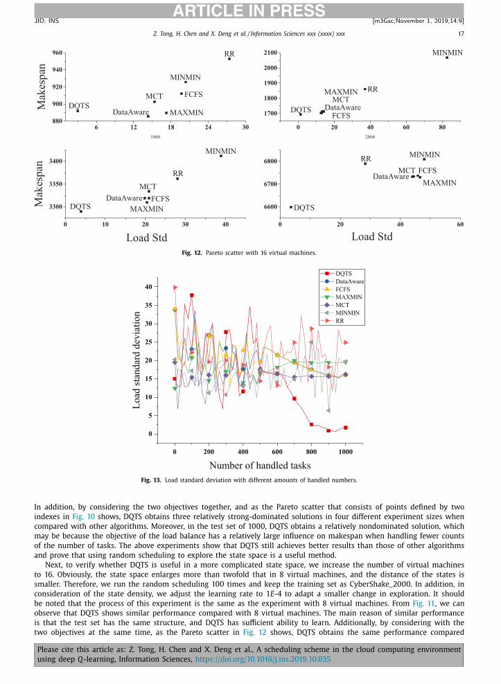
Fig. 12. Pareto scatter with 16 virtual machines.

Fig. 13. Load standard deviation with different amounts of handled numbers.

In addition, by considering the two objectives together, and as the Pareto scatter that consists of points defined by two

indexes in Fig. 10 shows, DQTS obtains three relatively strong-dominated solutions in four different experiment sizes when

compared with other algorithms. Moreover, in the test set of 10 0 0, DQTS obtains a relatively nondominated solution, which

may be because the objective of the load balance has a relatively large influence on makespan when handling fewer counts

of the number of tasks. The above experiments show that DQTS still achieves better results than those of other algorithms

and prove that using random scheduling to explore the state space is a useful method.

Next, to verify whether DQTS is useful in a more complicated state space, we increase the number of virtual machines

to 16. Obviously, the state space enlarges more than twofold that in 8 virtual machines, and the distance of the states is

smaller. Therefore, we run the random scheduling 100 times and keep the training set as CyberShake_20 0 0. In addition, in

consideration of the state density, we adjust the learning rate to 1 E -4 to adapt a smaller change in exploration. It should

be noted that the process of this experiment is the same as the experiment with 8 virtual machines. From Fig. 11 , we can

observe that DQTS shows similar performance compared with 8 virtual machines. The main reason of similar performance

is that the test set has the same structure, and DQTS has sufficient ability to learn. Additionally, by considering with the

two objectives at the same time, as the Pareto scatter in Fig. 12 shows, DQTS obtains the same performance compared





ARTICLE IN PRESS


Fig. 14. (a) Load standard deviation with test set of CyberShake. (b) Makespan with test set of CyberShake.

Fig. 15. (a) Load standard deviation with test set of Inspiral. (b) Makespan with test set of Inspiral.

with the situation of 8 virtual machines. However, it should be noted that the change in hyperparameters can cause a large

swing, and the process to select the hyperparameters needs more caution, such as when setting the learning rate to 1 E -4 or

another rate, and the performance will be greatly affected.

Next, to verify whether DQTS is useful in a more complicated state space, we increase the number of virtual machines to

16. The state space enlarges more than twofold that in 8 virtual machines, and the distance of the states is smaller. There-

fore, we run the random scheduling 100 times and keep the training set as CyberShake_20 0 0. Additionally, in consideration

of the state density, we adjust the learning rate to 1 E -4 to adapt a smaller change in exploration. It should be noted that

the process of this experiment is the same as the experiment with 8 virtual machines. From Fig. 11 , we can observe that

DQTS shows similar performance compared with 8 virtual machines. The main reason for this similar performance is that





ARTICLE IN PRESS


Table 3

Performance on benchmark of Inspiral_20 0 0.

Load Std Makespan

DQTS 190.0878655 30312.85

DataAware 157.7639315 30379.46

FCFS 157.9354705 30378.55

MAXMIN 238.6068311 30487.17

MCT 160.2887975 30366.20

MINMIN 185.9714359 30363.13

RR 216.4874891 30418.05

Table 4

Performance on benchmark of Montage_20 0 0.

Load Std Makespan

DQTS 32.17318958 1743.22

DataAware 70.93124509 1683.90

FCFS 70.93124509 1683.90

MAXMIN 71.04491097 1671.84

MCT 70.54326354 1681.13

MINMIN 70.15721547 1679.70

RR 71.08510002 1680.00

Table 5

Performance on benchmark of Sipht_20 0 0.

Load Std Makespan

DQTS 309.6397016 23928.19

DataAware 470.6224257 24838.23

FCFS 470.6224257 24838.23

MAXMIN 336.1103080 24546.45

MCT 564.8682626 25206.45

MINMIN 400.5922386 24867.65

RR 705.8387776 25176.95

the test set has the same structure, and DQTS has sufficient ability to learn. Additionally, by considering the two objectives

at the same time, as the Pareto scatter in Fig. 12 shows, DQTS obtains the same performance compared with the situation

of 8 virtual machines. However, it should be noted that the change in hyperparameters can cause a large swing, and the

process to select the hyperparameters needs more caution, such as when setting learning rate to 1 E -4 or another rate, and

the performance will be greatly affected.

To observe the real-time variance in the load balance, we design an experiment that calculates the load standard devi-

ation after each of a certain number of handled tasks. The variation curve with the increasing number of processed tasks

can be found in Fig. 13 . The figure shows that compared with other classic algorithms, the DQTS decreases in load std after

600 tasks because the upcoming tasks are relatively stable along with its length.

Additionally, we also know that DQTS reduces the instability and acquires a balanced final state. Therefore, we believe

that the DQTS algorithm is more suitable for dynamic online task scheduling in the cloud computing environment when

considering the load balance.

5.5. Performance on other benchmarks with the single-set model

In this section, we show the performance of a trained model that is generated in the above experiments with other

benchmarks on CyberShake. By training the NN 10 0,0 0 0 times, the model has already learned enough Markov decision pro-

cesses. To evaluate the performance of this model, it is necessary to test it with other benchmarks. We select Inspiral_20 0 0,

Montage_20 0 0 and Sipht_20 0 0 as the test sets. Table 5 shows that DQTS obtains relatively strong-dominated solutions with

Sipht_20 0 0, and Table 3 –4 shows relatively nondominated solutions with Inspiral_20 0 0 and Montage_20 0 0. We conclude

from Table 3 to 5 that the DQTS algorithm, when compared with other classic algorithms for various test sets, is better and

much more robust. Different benchmarks show its unique structure via the results recorded in the tables. In addition, DQTS

achieves relatively good solutions because of its adaptive capacity, containment and expandability when implemented in a

complex environment.

5.6. Performance on benchmarks with the hybrid-set model

We can see from the above experiments that each DAG benchmark still has differences. In addition, DQTS should have

the ability of containment and expandability. Thus, a hybrid training experiment should be conducted for this matter. We





ARTICLE IN PRESS


Fig. 16. (a) Load standard deviation with test set of Montage. (b) Makespan with test set of Montage.

run the random scheduling with CyberShake_20 0 0, Inspiral_20 0 0 and Montag_20 0 0 5 times separately. Then, we train the

set 10 0,0 0 0 times. As Figs. 14–16 shows, DQTS outperforms in the load std and makespan with different test sets. The results

show that DQTS maintains good containment and learning ability when the states become complex. Moreover, it should be

noted that using multiple types of training sets and a smaller train set has no impact on the results when compared to the

above CyberShake benchmark experiments. We can demonstrate that DQTS can adapt to even more complex environments

such as the multi-objective problem without the need for a more complex model to achieve its goal.

6. Conclusion and future work

In this paper, we have proposed a novel artificial intelligence algorithm, DQTS, to solve the problem of scheduling DAG

tasks in a cloud computing environment. According to experimental results, DQTS outperforms other algorithms and has

the advantages of excellent performance and a strong capability for learning, which proves that DQTS can be applied to task

scheduling in cloud computing environments, especially in complex environments. Additionally, we tested these algorithms

on WorkflowSim and processed them with scientific workflow benchmarks. The algorithm compares classic algorithms to

state-of-the-art algorithms under both makespan and load balance. The results show that DQTS obtains the lowest makespan

and best load-balance measurement.

In future works, we intend to propose a new model of energy consumption, which is an effective way to reduce costs

when the deadline is loose.

Declaration of Competing Interest

None.

Acknowlgedgments

The authors are grateful to the three anonymous reviewers for their constructive comments. The research was partially

funded by the Program of the National Natural Science Foundation of China (Grant No. 61502165 ) and the National Out-

standing Youth Science Program of the National Natural Science Foundation of China (Grant No. 61625202 ).

References

[1] Q. Wu , F. Ishikawa , Q. Zhu , Y. Xia , J. Wen , Deadline-constrained cost optimization approaches for workflow scheduling in clouds, IEEE Trans. Parallel

Distrib. Syst. 28 (12) (2017) 3401–3412 . [2] J.H. Holland , Adaptation in Natural and Artificial Systems, MIT Press, 1992 .

[3] L. Baxter , Markov decision processes: discrete stochastic dynamic programming, Technometrics 37 (3) (2009) 353 . [4] C.J. Watkins , P. Dayan , Q-learning, Mach. Learn. 8 (3–4) (1992) 279–292 .



https://doi.org/10.13039/501100001809

https://doi.org/10.13039/501100001809

http://refhub.elsevier.com/S0020-0255(19)30997-1/sbref0001















ARTICLE IN PRESS


[5] Z. Tong , X. Deng , H. Chen , J. Mei , H. Liu , QL-HEFT: a novel machine learning scheduling scheme base on cloud computing environment, Neural Comput.Appl. (2019) 1–18 .

[6] R. Lu , S.H. Hong , X. Zhang , A dynamic pricing demand response algorithm for smart grid: reinforcement learning approach, Appl. Energy 220 (2018)220–230 .

[7] Y. Yang , J. Hao , M. Sun , Z. Wang , C. Fan , G. Strbac , Recurrent deep multiagent q-learning for autonomous brokers in smart grid., in: International JointConference on Artificial Intelligence, vol. 18, 2018, pp. 569–575 .

[8] Y. Yang , J. Hao , Z. Wang , M. Sun , G. Strbac , Recurrent deep multiagent q-learning for autonomous agents in future smart grid, in: Proceedings of

the 17th International Conference on Autonomous Agents and MultiAgent Systems, International Foundation for Autonomous Agents and MultiagentSystems, Richland, SC, 2018, pp. 2136–2138 .

[9] H. Wang , Y. Wu , G. Min , Data-driven dynamic resource scheduling for network slicing: A Deep reinforcement learning approach, Inf. Sci. 498 (2019)106–116 .

[10] D. Garg , M. Chli , G. Vogiatzis , Deep Reinforcement Learning for Autonomous Traffic Light Control, 2018 3rd IEEE International Conference on IntelligentTransportation Engineering (ICITE), IEEE, 2018, pp. 214–218 .

[11] V. Mnih , K. Kavukcuoglu , D. Silver , A .A . Rusu , J. Veness , M.G. Bellemare , A. Graves , M. Riedmiller , A.K. Fidjeland , G. Ostrovski , et al. , Human-levelcontrol through deep reinforcement learning, Nature 518 (7540) (2015) 529–533 .

[12] H. Topcuoglu , S. Hariri , M.Y. Wu , Performance-effective and low-complexity task scheduling for heterogeneous computing, IEEE Trans. Parallel Distrib.

Syst. 13 (3) (2002) 260–274 . [13] K. Li , X. Tang , B. Veeravalli , K. Li , Scheduling precedence constrained stochastic tasks on heterogeneous cluster systems, IEEE Trans. Comput. 64 (1)

(2014) 191–204 . [14] H. Arabnejad , J.G. Barbosa , List scheduling algorithm for heterogeneous systems by an optimistic cost table, IEEE Trans. Parallel Distrib. Syst. 25 (3)

(2014) 682–694 . [15] N. Zhou , D. Qi , X. Wang , Z. Zheng , W. Lin , A list scheduling algorithm for heterogeneous systems based on a critical node cost table and pessimistic

cost table, Concurrency Comput. Pract. Experience 29 (5) (2017) 1–11 .

[16] J.J. Durillo , R. Prodan , Multi-objective workflow scheduling in amazon EC2, Cluster Comput. 17 (2) (2014) 169–189 . [17] A. Gerasoulis , T. Yang , A comparison of clustering heuristics for scheduling directed acyclic graphs on multiprocessors, J. Parallel Distrib. Comput. 16

(4) (1992) 276–291 . [18] R. Bajaj , D.P. Agrawal , Improving scheduling of tasks in a heterogeneous environment, IEEE Trans. Parallel Distrib. Syst. 15 (2) (2004) 107–118 .

[19] G. Xie , R. Li , K. Li , Heterogeneity-driven end-to-end synchronized scheduling for precedence constrained tasks and messages on networked embeddedsystems, J. Parallel Distrib. Comput. 83 (2015) 1–12 .

[20] Z. Tong , H. Chen , X. Deng , K. Li , K. Li , A novel task scheduling scheme in a cloud computing environment using hybrid biogeography-based optimiza-

tion, Soft Comput. 23 (21) (2019) 11035–11054 . [21] A. Liang , Y. Pang , A novel, energy-aware task duplication-based scheduling algorithm of parallel tasks on clusters, Math. Comput. Appl. 22 (1) (2017)

1–12 . [22] D. Bozdag , F. Ozguner , U.V. Catalyurek , Compaction of schedules and a two-stage approach for duplication-based DAG scheduling, IEEE Trans. Parallel

Distrib. Syst. 20 (6) (2009) 857–871 . [23] L. Teylo , U. de Paula , Y. Frota , D. de Oliveira , L.M. Drummond , A hybrid evolutionary algorithm for task scheduling and data assignment of data-inten-

sive scientific workflows on clouds, Future Gener. Comput. Syst. 76 (2017) 1–17 .

[24] M. Wang , J. Zhang , F. Dong , J. Luo , Data placement and task scheduling optimization for data intensive scientific workflow in multiple data centersenvironment, in: Advanced Cloud and Big Data (CBD), 2014 Second International Conference on, IEEE, 2014, pp. 77–84 .

[25] H. Arabnejad , J.G. Barbosa , Multi-QoS constrained and profit-aware scheduling approach for concurrent workflows on heterogeneous systems, FutureGener. Comput. Syst. 68 (2017) 211–221 .

[26] H. Zhao , R. Sakellariou , Scheduling multiple dags onto heterogeneous systems, in: Parallel and Distributed Processing Symposium, 2006. IPDPS 2006.20th International, IEEE, 2006, pp. 14–20 .

[27] H. Kanemitsu , M. Hanada , H. Nakazato , Prior node selection for scheduling workflows in a heterogeneous system, J. Parallel Distrib. Comput. 109 (2017)

155–177 . [28] H. Chen , J. Zhu , Z. Zhang , M. Ma , X. Shen , Real-time workflows oriented online scheduling in uncertain cloud environment, J. Supercomput. 73 (11)

(2017) 4 906–4 922 . [29] L. Zhang , K. Li , Y. Xu , J. Mei , F. Zhang , K. Li , Maximizing reliability with energy conservation for parallel task scheduling in a heterogeneous cluster,

Inf. Sci. 319 (2015) 113–131 . [30] Y. Wei , L. Pan , S. Liu , L. Wu , X. Meng , DRL-Scheduling: an intelligent QoS-aware job scheduling framework for applications in clouds, IEEE Access 6

(2018) 55112–55125 .

[31] Q. Zhang , M. Lin , L.T. Yang , Z. Chen , P. Li , Energy-efficient scheduling for real-time systems based on deep q-learning model, IEEE Trans. SustainableComput. 4 (1) (2017) 132–141 .

[32] J. Jiang , Y. Lin , G. Xie , L. Fu , J. Yang , Time and energy optimization algorithms for the static scheduling of multiple workflows in heterogeneouscomputing system, J. Grid Comput. 15 (4) (2017) 435–456 .

[33] Z. Wang , Z. Wei , Dynamic engineering multi-criteria decision making model optimized by entropy weight for evaluating bid, Syst. Eng. Procedia 5(2012) 49–54 .

[34] X. Tang , X. Li , Z. Fu , Budget-constraint stochastic task scheduling on heterogeneous cloud systems, Concurrency Comput. 29 (19) (2017) e4210 . [35] F.S. Melo , Convergence of Q-learning: A Simple Proof, Tech. Rep., Institute of Systems and Robotics, 2001 .

[36] J. Nie , S. Haykin , A q-learning-based dynamic channel assignment technique for mobile communication systems, IEEE Trans. Veh. Technol. 48 (5)

(1999) 1676–1687 . [37] G. Taylor , R. Parr , Kernelized value function approximation for reinforcement learning, in: International Conference on Machine Learning, 2009,

pp. 1017–1024 . [38] X. Xu , Z. Huang , D. Graves , W. Pedrycz , A clustering-based graph Laplacian framework for value function approximation in reinforcement learning,

IEEE Trans. Cybern. 44 (12) (2014) 2613–2625 . [39] S. Mahadevan , M. Maggioni , Proto-value functions: a Laplacian framework for learning representation and control in Markov decision processes, J.

Mach. Learn. Res. 8 (Oct) (2007) 2169–2231 .

[40] M. Cheng , J. Li , S. Nazarian , DRL-cloud: deep reinforcement learning-based resource provisioning and task scheduling for cloud service providers, in:Proceedings of the 23rd Asia and South Pacific Design Automation Conference, 2018, pp. 129–134 .

[41] B. Zhang , C. Liu , J. Tang , Learning-based energy-efficient data collection by unmanned vehicles in smart cities, IEEE Transactions on Industrial Infor-matics 14 (4) (2017) 1666–1676 .

[42] yenchenlin, ( https://github.com/yenchenlin/DeepLearningFlappyBird ). [43] S. Bharathi , A. Chervenak , E. Deelman , G. Mehta , M.H. Su , K. Vahi , Characterization of scientific workflows, in: Workflows in Support of Large-Scale

Science, 2008. WORKS 2008. Third Workshop on, 2008, pp. 1–10 .

[44] R.F.D. Silva , W. Chen , G. Juve , K. Vahi , E. Deelman , Community resources for enabling research in distributed scientific workflows, in: IEEE InternationalConference on E-Science, 2014, pp. 177–184 .

[45] G. Juve , A. Chervenak , E. Deelman , S. Bharathi , G. Mehta , K. Vahi , Characterizing and profiling scientific workflows, Future Gener. Comput. Syst. 29 (3)(2013) 682–692 .


























http://refhub.elsevier.com/S0020-0255(19)30997-1/othref0001



















































































































































https://github.com/yenchenlin/DeepLearningFlappyBird























ARTICLE IN PRESS


[46] R.N. Calheiros , R. Ranjan , A. Beloglazov , C.A.F.D. Rose , R. Buyya , CloudSim: a toolkit for modeling and simulation of cloud computing environmentsand evaluation of resource provisioning algorithms, Softw. Pract. Experience 41 (1) (2010) 23–C50 .

[47] W. Chen , E. Deelman , WorkflowSim: a toolkit for simulating scientific workflows in distributed environments, in: IEEE International Conference onE-Science, 2013, pp. 1–8 .

[48] E. Deelman , K. Vahi , G. Juve , M. Rynge , S. Callaghan , P.J. Maechling , R. Mayani , W. Chen , R.F. Da Silva , M. Livny , et al. , Pegasus, a workflow managementsystem for science automation, Future Gener. Comput. Syst. 46 (2015) 17–35 .

[49] K. Deb , A. Pratap , S. Agarwal , T. Meyarivan , A fast and elitist multiobjective genetic algorithm: NSGA-II, IEEE Trans. Evol. Comput. 6 (2) (2002) 182–197 .






























a scheduling scheme in the cloud computing environment

Documents