a satellite approach to estimate land–atmosphere 2

IEEE TRANSACTIONS ON GEOSCIENCE AND REMOTE SENSING , VOL. 47, NO. 2, FEBRUARY 2009 569

A Satellite Approach to Estimate Land–AtmosphereCO2 Exchange for Boreal and Arctic Biomes

Using MODIS and AMSR-EJohn S. Kimball, Member, IEEE, Lucas A. Jones, Student Member, IEEE, Ke Zhang, Faith Ann Heinsch,

Kyle C. McDonald, Senior Member, IEEE, and Walt C. Oechel

Abstract—Northern ecosystems are a major sink for atmo-spheric CO2 and contain much of the world’s soil organic carbon(SOC) that is potentially reactive to near-term climate change.We introduce a simple terrestrial carbon flux (TCF) model drivenby satellite remote sensing inputs from the Moderate Resolu-tion Imaging Spectroradiometer (MODIS) and the Advanced Mi-crowave Scanning Radiometer for EOS (AMSR-E) to estimatesurface (< 10-cm depth) SOC stocks, daily respiration, and netecosystem carbon exchange (NEE). Soil temperature and moistureinformation from AMSR-E provide environmental constraints tosoil heterotrophic respiration (Rh), while gross primary pro-duction (GPP) information from MODIS provides estimates ofthe total photosynthesis and autotrophic respiration. The modelresults were evaluated across a North American network of borealforest, grassland, and tundra monitoring sites using alternativecarbon measures derived from tower CO2 flux measurements andBIOME-BGC model simulations. Root-mean-square-error (rmse)differences between TCF model estimates and tower observationswere 1.2, 0.7, and 1.2 g · C · m−2 · day−1 for GPP, ecosystemrespiration (Rtot) and NEE, while mean residual differenceswere 43% of the rmse. Similar accuracies were observed forboth TCF and BIOME-BGC model simulations relative to towerresults. TCF-model-derived SOC was in general agreement withsoil inventory data and indicates that the dominant SOC sourcefor Rh has a mean residence time of less than five years, whileRh is approximately 43% and 55% of Rtot for respective sum-mer and annual fluxes. An error sensitivity analysis determinedthat meaningful flux estimates could be derived under prevailingclimatic conditions at the study locations, given documented errorlevels in the remote sensing inputs.

Index Terms—Advanced Microwave Scanning Radiometer forEOS (AMSR-E), Arctic tundra, boreal forest, carbon, ModerateResolution Imaging Spectroradiometer (MODIS), net ecosystemexchange (NEE).

Manuscript received March 17, 2008; revised May 19, 2008 and June 17,2008. First published December 2, 2008; current version published January 28,2009. This work was supported in part by the National Aeronautics and SpaceAdministration’s Earth Science Enterprise and in part by the National ScienceFoundation’s Office of Polar Programs through grants.

J. S. Kimball, L. A. Jones, and K. Zhang are with the Flathead Lake Biologi-cal Station, Division of Biological Sciences, The University of Montana (UM),Polson, MT 59860-6815 USA, and also with the Numerical Terradynamic Sim-ulation Group, UM, Missoula, MT 59812 USA (e-mail: [email protected];[email protected]; [email protected]).

F. A. Heinsch is with the Numerical Terradynamic Simulation Group,The University of Montana, Missoula, MT 59812 USA (e-mail: [email protected]).

K. C. McDonald is with the Water and Carbon Cycles Group, Science Divi-sion, Jet Propulsion Laboratory, California Institute of Technology, Pasadena,CA 91109 USA (e-mail: [email protected]).

W. C. Oechel is with the Global Change Research Group, Department ofBiology, San Diego State University, San Diego, CA 92182 USA (e-mail:[email protected]).

Color versions of one or more of the figures in this paper are available onlineat http://ieeexplore.ieee.org.

Digital Object Identifier 10.1109/TGRS.2008.2003248

NOMENCLATURE

AMSR-E Advanced Microwave Scanning Radio-meter for EOS.

BIOME-BGC BIOME-BioGeochemicalCycles(BGC)model.

BPLUT Biome property lookup table.Cmet, Cstr, and Crec Metabolic, structural, and recalcitrant

SOC pools, respectively.GMAO NASA Global Modeling and Assimila-

tion Office.GPP Gross primary production (GPP > 0

denotes photosynthetic uptake).MODIS Moderate Resolution Imaging Spectro-

radiometer.MR Mean residual error.NCEP–NCAR National Centers for Environmental

Prediction–National Center for Atmos-pheric Research.

NEE Net ecosystem carbon exchange(NEE < 0 denotes ecosystem uptake).

NPP Net primary production (NPP > 0 de-notes ecosystem uptake).

Ra Autotrophic respiration (Ra > 0 de-notes respiratory losses).

Rh Heterotrophic respiration (Rh > 0 de-notes respiratory losses).

rmse Root-mean-square error.Rtot Total ecosystem respiration (Rtot > 0

denotes respiratory losses).SM Soil moisture expressed as a proportion

of relative saturation.SOC Soil organic carbon.Tb Microwave brightness temperature.TCF Terrestrial carbon flux model.

I. INTRODUCTION

NORTHERN high-latitude boreal and Arctic biomes areimportant components of the global carbon cycle because

they constitute a major sink for anthropogenic CO2 emissionsand contain approximately 119 Pg of soil organic carbon (SOC)that is potentially reactive in the context of near-term climatechange [1], [2]. Recent studies and long-term measurementrecords indicate that much of the region is becoming warmer[3] and drier [4]–[6] with recent declines in carbon sink strength

0196-2892/$25.00 © 2008 IEEE

Authorized licensed use limited to: Jet Propulsion Laboratory. Downloaded on January 12, 2010 at 19:28 from IEEE Xplore. Restrictions apply.

570 IEEE TRANSACTIONS ON GEOSCIENCE AND REMOTE SENSING , VOL. 47, NO. 2, FEBRUARY 2009

[7], [8]. Current and projected regional warming trends mayexacerbate global climate change by destabilizing regional SOCstocks and reducing the capacity of northern ecosystems tosequester atmospheric CO2.

The net ecosystem exchange (NEE) of carbon (CO2) withthe atmosphere is the residual difference between carbon uptakeby vegetation gross primary production (GPP) and carbon lossthrough autotrophic and heterotrophic respiration, collectivelytermed ecosystem respiration. The NEE term is thus a usefulmeasure of the magnitude and direction of carbon flow betweenecosystems and the atmosphere [9]. Current capabilities forregional assessment and monitoring of NEE for boreal–Arcticecosystems are limited. Atmospheric transport model inver-sions of CO2 concentrations from sparse measurement stationsprovide information on seasonal patterns and trends in at-mospheric CO2 but little information on underlying processes;these methods are also too coarse to resolve carbon-source–sinkactivity at scales finer than broad latitudinal and continentaldomains [8], [10]. Tower CO2 flux measurement networksprovide detailed information on stand-level NEE and associatedbiophysical processes, but little information regarding spatialvariability in these processes over heterogeneous landscapes[11]. Alternative measures of NEE and component carbonfluxes from satellite remote sensing potentially provide themeans for scaling between relatively intensive stand-level mea-surement and modeling approaches, and top–down assessmentsfrom atmospheric model inversions.

The Moderate Resolution Imaging Spectroradiometer(MODIS) onboard the NASA EOS Terra and Aqua satelliteshas been providing global operational mapping of GPP atapproximate eight-day intervals since 2000 and 2002, respec-tively [12]. The GPP term quantifies the photosynthetic uptakeof atmospheric CO2 but represents an incomplete picture ofNEE because of a lack of information on ecosystem respiration.Several studies have applied satellite remote sensing to char-acterize NEE over boreal–Arctic landscapes using empiricalrelationships between CO2 flux measurements and spectralvegetation indices [13], [14] or simple physiological modelsdriven by optical–infrared (IR) remote sensing and surfacemeteorological data to characterize both vegetation productivityand ecosystem respiration [15], [16]. Empirical approachesare constrained to the specific regions and conditions underwhich they were developed and provide little diagnostic insightinto underlying biophysical processes. Physiological modelsattempt to account for the primary environmental constraints onproductivity and respiration but are often limited by the avail-ability and resolution of driving meteorological data sets fromsparse observational networks or coarse (1◦–2.5◦) resolutiongridded products from atmospheric model reanalyses. Recentdevelopments in satellite remote sensing offer the potentialfor direct measurement and improved resolution of environ-mental constraints for estimating land–atmosphere carbonexchange.

Satellite microwave radiometers are sensitive to variationsin surface emissivity and dielectric constant associated withchanges in soil moisture (SM) and temperature [17], [18].Lower frequency microwaves (e.g., < 18.7 GHz) are capableof penetrating clouds and low-biomass vegetation to provide

information more representative of the underlying soil thanhigh frequency microwave and thermal IR observations. Thesefavorable properties have been exploited for mapping surfaceSM and temperature across a wide range of environmentsand vegetation types, including boreal forest and tundra [19],[20]. The Advanced Microwave Scanning Radiometer for EOS(AMSR-E) is deployed with MODIS on the Aqua satellite andhas been providing global multifrequency brightness tempera-ture measurements on a daily basis since 2002. Current AMSR-E operational and experimental products include daily SM [18]and soil temperature [20], offering potential surrogate measuresof SM and temperature controls to heterotrophic respiration.Thus, synergistic information from MODIS and AMSR-E mayprovide an alternative means for regional mapping and mon-itoring of NEE and component GPP and respiration fluxes.The relatively coarse (∼25-km) spatial scale of the AMSR-E footprint limits the ability of the sensor to resolve subgrid-scale land surface properties. However, the utility of satellitemicrowave remote sensing for northern latitudes is the abilityto monitor land surface conditions day or night, independent ofsolar illumination or signal degradation from cloud cover andother atmospheric aerosol effects.

We introduce a new satellite remote sensing algorithm fordetermining NEE and component carbon fluxes for boreal andArctic ecosystems using synergistic biophysical informationfrom MODIS and AMSR-E. Remote sensing inputs to thealgorithm include land-cover class and GPP information fromMODIS for characterizing general ecosystem properties and netphotosynthetic uptake of CO2, and daily surface soil temper-ature and moisture information from AMSR-E for estimatingsoil decomposition and heterotrophic respiration. A by-productof the algorithm initialization process includes a regional esti-mation of surface (< 10-cm depth) SOC stocks. The algorithmresults are evaluated across a North American network of borealforest, grassland (GRS), and tundra monitoring sites usingindependent measures of GPP, ecosystem respiration, and NEEderived from BIOME-BioGeochemical Cycles (BGC) ecosys-tem process model simulations and tower eddy covariance CO2

flux measurements. The objectives of this paper are to char-acterize algorithm uncertainty and determine whether globaloperational satellite remote sensing products can be appliedwithin a simple carbon model framework to determine NEE andcomponent GPP and respiration fluxes with similar accuracy asmore detailed ecosystem process model simulations.

II. APPROACH

A. Study Domain and Test Sites

We selected nine study sites for this investigation, en-compassing North American tundra, boreal forest, and GRSecosystems across a latitudinal climate and vegetation biomassgradient. The sites coincide with existing or previous towereddy covariance CO2 flux measurement campaigns and rep-resent five distinct local vegetation types, including coastalwet-sedge tundra, moist tussock tundra, boreal evergreenneedleleaf forest (ENLF), boreal deciduous broadleaf forest,and northern temperate GRS (see Table I and Fig. 1). The


KIMBALL et al.: SATELLITE APPROACH TO ESTIMATE LAND–ATMOSPHERE CO2 EXCHANGE FOR BIOMES 571

TABLE IBOREAL FOREST, GRASSLAND, AND TUNDRA STUDY SITES USED FOR TCF MODEL ASSESSMENT

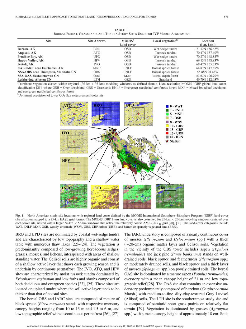
Fig. 1. North American study site locations with regional land cover defined by the MODIS International Geosphere–Biosphere Program (IGBP) land-coverclassification mapped to a 25-km EASE grid format. The MODIS IGBP 1-km land cover is also presented for 25-km × 25-km modeling windows centered overeach tower site, nested within larger 56-km × 56-km windows that reflect the relatively coarse AMSR-E TB grid [20], [30]. The land-cover categories includeWAT, ENLF, MXF, OSB, woody savannah (WSV), GRS, CRP, urban (URB), and barren or sparsely vegetated land (BRN).

BRO and UPD sites are dominated by coastal wet-sedge tundraand are characterized by low topography and a shallow watertable with numerous thaw lakes [22]–[24]. The vegetation ispredominantly composed of low-growing herbaceous sedges,grasses, mosses, and lichens, interspersed with areas of shallowstanding water. The Gelisol soils are highly organic and consistof a shallow active layer that thaws each growing season and isunderlain by continuous permafrost. The IVO, ATQ, and HPVsites are characterized by moist tussock tundra dominated byEriophorum vaginatum and low forbs and shrubs composed ofboth deciduous and evergreen species [23], [25]. These sites arelocated on upland tundra where the soil active layer tends to bethicker than that of coastal sites.

The boreal OBS and IARC sites are composed of mature ofblack spruce (Picea mariana) stands with respective overstorycanopy heights ranging from 10 to 13 m and 1.5 to 6 m, andlow topographic relief with discontinuous permafrost [26], [27].

The IARC understory is composed of a nearly continuous coverof mosses (Pleurozium and Hylocomium spp.) with a thick(∼20-cm) organic matter layer and Gelisol soils. Vegetationin the vicinity of the OBS tower includes aspen (Populoustremuloides) and jack pine (Pinus banksiana) stands on well-drained soils, black spruce and feathermoss (Pleurozium spp.)on moderately drained soils, and black spruce and a thick layerof mosses (Sphagnum spp.) on poorly drained soils. The borealOAS site is dominated by a mature aspen (Populus tremuloides)overstory with a mean canopy height of 21 m and low topo-graphic relief [28]. The OAS site also contains an extensive un-derstory predominantly composed of hazelnut (Corylus cornutaMarsh.) with medium-to-fine silty-clay-textured Gray Luvisol(Alfisol) soils. The LTH site is the southernmost study site andis composed of semiarid short-grass prairie on relatively flatterrain [29]. Vegetation is dominated by grasses (Agropyronspp.) with a mean canopy height of approximately 18 cm. Soils



at the LTH site are composed of orthic dark-brown chernozems(Mollisols) with a clay loam texture.

We identified the dominant land-cover class within overlying25-km × 25-km windows surrounding each site location usingthe MODIS IGBP global land-cover classification [21]. In mostcases, the local vegetation was of a similar functional typeas the overlying global land-cover classification. The tundrasites were identified as open shrubland (OSB) by the land-cover classification. The BRO1 and BRO2 tower locationsare within 1 km of each other and were represented withinthe same regional window. The OBS and IARC sites wereclassified as ENLF, while the LTH site was classified as GRS.The aspen-dominated OAS tower footprint differed from theregional land cover, which was classified as mixed evergreenneedleleaf and broadleaf deciduous forest (MXF) due to therelative abundance of both vegetation functional types withinthe regional modeling window.

B. Model Development

We applied a simple terrestrial carbon flux (TCF) modelto compute ecosystem respiration and NEE on a daily basis.Our approach has structural elements similar to the Century[31], [32] and CASA [33] soil decomposition models but isadapted for use with daily biophysical inputs derived from bothsatellite optical–IR and passive microwave remote sensing timeseries as primary model drivers. Model inputs include dailyGPP, soil temperature, and SM. GPP is used to estimate veg-etation net primary production (NPP), autotrophic respiration,and metabolic, structural, and recalcitrant SOC pools. Surface(< 10-cm depth) soil temperature and moisture inputs are usedto define the environmental controls to soil decomposition andheterotrophic respiration. Static inputs to the model includea global land-cover classification, which is used within theframework of a general biome properties lookup table (BPLUT)to define physiological response characteristics of differentvegetation classes. All model inputs represent satellite-remote-sensing-derived products from NASA EOS sensors.

NEE (in grams of carbon per square meter per day) iscomputed on a daily basis as the residual difference betweenGPP and respiration from autotrophic (Ra) and heterotrophic(Rh) components

NEE = (Ra + Rh) − GPP (1)

where positive (+) and negative (−) NEE fluxes denote therespective terrestrial loss or uptake of CO2. The GPP term (ingrams of carbon per square meter per day) represents the meanvegetation GPP of the dominant land-cover class within a gridcell and is obtained as an external model input. The Ra termencompasses growth and maintenance respiration componentsand is computed on a daily basis as a fixed proportion of GPPwithin individual land-cover classes, based on observationalevidence that the ratio of Ra to GPP is conserved across globalbiomes [34]–[36]. While this assumption provides a key simpli-fication for a remote sensing algorithm, the proportion of plantphotosynthesis devoted to biophysical growth and maintenance

may vary under changing environmental conditions and overthe course of vegetation development [37]–[39].

Heterotrophic respiration is computed as the sum of variabledecomposition and respiration rates from three distinct carbonpools as

Rh = (KmetCmet + KstrCstr + KrecCrec) (2)

where Cmet, Cstr, and Crec (in grams of carbon per squaremeter) represent metabolic, structural, and recalcitrant SOCpools, and Kmet, Kstr, and Krec (per day) are the corre-sponding decomposition rate parameters. The metabolic andstructural SOC pools represent plant litter with relatively short(e.g., less than or equal to five years) turnover periods, whilethe recalcitrant pool represents more physically and chemicallyprotected SOC with a longer turnover time.

The three-pool soil decomposition model approach is a sim-ple approximation of the complex variation of intrinsic SOCturnover rates but has been found to produce results consistentwith a wide range of observations from soil warming andincubation experiments [40]. Annual inputs to the Cmet andCstr pools in (2) are derived as proportions of annual NPP,and input to Crec is a constant fraction of the Cstr pool; outputsto these SOC pools represent the annual sums of respiredcomponents from (2)

dCmet/dt =CfractNPP − Rh,met (3)

dCstr/dt = (1 − Cfract)NPP − 0.7Cstr − Rh,str (4)

dCrec/dt = 0.7Cstr − Rh,rec (5)

where NPP is estimated as a fixed proportion of annual GPP(in grams of carbon per square meter per year) for individualland-cover classes, based on the assumption of conservatismin vegetation-carbon-use efficiency (i.e., NPP/GPP) and theproportional allocation of GPP to Ra within global biomes[34]–[36]. The Cfract term defines the rate in which NPP is al-located to metabolic and structural SOC pools, and is specifiedas a fixed rate within individual land-cover classes [32], [33].Values for Cfract, and proportional allocations of GPP to Ra

and NPP are defined in a BPLUT of general ecophysiologicalproperties of each land-cover class (Table II). This approach isbased on the assumption that the litter input to the SOC poolis proportional to NPP under long-term steady-state conditions[31], [32].

The TCF model uses dimensionless rate curves to account forsoil temperature and moisture constraints to soil decomposition.The soil decomposition rate (K) is derived as the productof dimensionless multipliers for soil temperature (Tmult) andmoisture (Wmult) and a theoretical maximum rate constant(Kmx; per day) under prevailing climate conditions

K = KmxTmultWmult (6)

where K is equivalent to Kmet, and Tmult and Wmult varybetween zero and one. The value for Kmx was specified as aconstant rate (0.0301 per day) for all biomes, while decompo-sition rate parameters for Kstr and Krec were estimated as 40%and 1% of Kmet, respectively [32]. The estimation of K in (6)



TABLE IIGENERAL BPLUT DESCRIBING SITE ECOPHYSIOLOGICAL

PARAMETERS FOR TCF MODEL CALCULATIONS

assumes constant soil decomposer efficiency (microbial-CO2-production-to-carbon-assimilation ratio) inherent in the Kmx

term, and that SM and temperature are the dominant controlson near-term (daily, seasonal, and annual) decomposition rates.However, we assume that changes in litter quality (e.g., physicalprotection and/or chemical resistance to microbial decompo-sition) influence Rh and NEE indirectly through associatedchanges in satellite-remote-sensing-derived GPP inputs overgenerally N-limited boreal and tundra ecosystems.

The soil decomposition rate response to temperature is de-fined using an Arrhenius-type function following [41]

Tmult = exp[308.56

((66.02)−1 − (Ts,k − 227.13)−1

)](7)

where (7) is expressed relative to a 20-◦C reference temperatureand Ts,k is the surface soil temperature (in kelvins). A varietyof functional types have been used to describe temperatureeffects on soil respiration, including exponential [42], [43] andPoisson [31], [32] functions, while the Arrhenius functionaltype is physically based and provides a relatively accurateand unbiased estimate of soil respiration across a wide rangeof biome types and environmental conditions [40], [41], [44].We assume that for soil temperatures above a 20-◦C referencestate, Tmult is unity, and temperature is no longer limiting tosoil decomposition. Under these conditions, SM is expected todecline with warmer soil temperatures, and Wmult becomes theprimary constraint to K.

The soil decomposition rate response to SM has been de-scribed using quadratic and parabolic functions and varyingexpressions of soil water content, with optimum rates beingat intermediate soil water levels [45]. For this investigation,the soil decomposition rate response to SM is represented asa parabolic function

Wmult = 0.00036(105.0 SM − SM)2 (8)

where SM is expressed as a proportion (in percent) of satura-tion. The parabolic response curve accounts for the inhibitoryeffects of both low and high soil water on heterotrophic res-piration rates and is consistent with laboratory soil incubationstudies and field observations for a range of global biome types,including GRS and tundra [46]–[49]. The SM limitation todecomposition described by (8) approaches unity near 50% of

soil saturation, although the shape of the parabolic response islikely to vary across different biomes and soil types. For this in-vestigation, we assume that mean surface soil properties withinboreal and arctic biomes are similar at the relatively coarse(∼25-km) spatial resolution of satellite-microwave-remote-sensing-derived SM inputs.

C. TCF Model Inputs

The TCF model requires time series inputs of daily GPP,surface soil temperature, and SM to compute ecosystem res-piration and NEE on a daily basis. Model inputs were de-rived using a three-year (2002–2004) daily time series of GPP,soil temperature, and SM derived from MODIS and AMSR-Esensor records. A MODIS global land-cover classification [21]was used with the BPLUT in Table II to define general eco-physiological properties for each of the study sites; the BPLUTparameters were derived from the literature for boreal, GRS,and tundra ecosystems. For each site window, the Cmet, Cstr,and Crec pools were initialized to steady-state conditions bycontinuous cycling of the three-year GPP, soil temperature, andSM daily time series.

1) GPP: The NASA MODIS has been operational on theNASA EOS Terra and Aqua satellites since 2000 and 2002, re-spectively, and provides a variety of consistent, well-calibrated,and validated land surface information ranging from spectralradiance and reflectance data to derived higher order bio-physical variables including land-cover type, canopy photo-synthetic leaf area, and vegetation productivity. Model GPPinputs were derived from the MODIS MOD17A2 algorithm[12]. The MOD17A2 algorithm has undergone several majorrevisions in response to extensive ongoing calibration andverification studies using biophysical information from regionalstation networks, including boreal and Arctic landscapes (e.g.,[50]–[53]). For this investigation, we use the fifth-generation(Collection 5) version of the MOD17A2 algorithm and associ-ated MOD15 LAI and FPAR inputs [52], [54]. The MOD17A2algorithm uses a production efficiency model with MODISsensor-derived land cover, fractional photosynthetically activeradiation (FPAR), leaf area index (LAI), and daily surface me-teorology as primary drivers. Daily surface meteorology inputsinclude incident solar radiation (SWrad), minimum and meandaily air temperatures (Tmin and Tavg, respectively), and at-mospheric vapor pressure deficit (VPD), which are provided bythe NASA Global Modeling and Assimilation Office (GMAO)reanalysis surface meteorology [55], [56]. The surface meteo-rological data are used with simple response curves to estimateenvironmental reductions in photosynthetic-light-use efficiencyunder suboptimal solar radiation, temperature, and humidityconditions. The biophysical characteristics of the land surfacevary according to individual land-cover classes as defined usinga 1-km-resolution global land-cover map and the MOD17A2BPLUT [52]. GPP is derived globally on a daily basis at 1-kmspatial resolution and composited over eight-day time intervals.

We also used an alternative MOD17A2 product developedusing daily surface meteorological inputs from the NationalCenters for Environmental Prediction–National Center forAtmospheric Research (NCEP–NCAR) reanalysis (NNR) [6].



The MOD17-NNR and MOD17-GMAO products differ in thatthe NNR surface air temperature, solar radiation, and VPD datahave been corrected for regional bias using daily observationsfrom the pan-boreal regional surface weather station network.Both MODIS data sets are used in this investigation to assessTCF model sensitivity to alternative GPP inputs.

The MODIS GPP inputs are derived globally at 1-km spatialresolution and eight-day intervals. The eight-day 1-km MODISFPAR/LAI data used for these calculations are screened toremove cloud contamination and snow effects indicated by thedaily MOD15A2 QC fields [52]. The GPP data were resampledto a daily time step by temporal linear interpolation of adjacenteight-day values. The GPP values were then aggregated to a25-km spatial resolution by averaging values of the domi-nant land-cover class indicated by the MODIS 1-km-resolutionglobal land-cover classification within each 25-km grid cell.The data were then reprojected to a 25-km polar EASE gridcentered over each study site location using a nearest neighborresampling scheme.

2) SM and Temperature: Daily soil temperature inputs werederived using multifrequency dual-polarized Level-2A (L2A)brightness temperatures (Tb)’s from AMSR-E [57], [20]. TheAMSR-E sensor measures brightness temperatures at 6.9-,10.7-, 18.7-, 23.8-, 36.5-, and 89-GHz frequencies. The na-tive resolution of each frequency ranges from approximately5 km × 5 km at 89 GHz to 60 km × 60 km at 6.9 GHz. TheL2A data represent Tb from all frequencies resampled to the6.9-GHz 60-km × 60-km native resolution [57]. The Aquasatellite is polar-orbiting with 1-A.M./P.M. equatorial crossingtimes, providing multiple daily acquisitions in polar regions[58]. For high-latitude regions, the overlapping orbital swathsallow two to four Tb observations per footprint overpass witha typical standard deviation of approximately 1 K (max =5 K) at 6.9 GHz and < 1 K (max = 3.5 K) at 89 GHz. TheTb observations were extracted from Level-2A orbital swathfootprints whose centroid falls within 5 km of each site location.Therefore, the observations can be considered to be represen-tative of an approximate 60-km × 60-km pixel centered overeach location. The descending (A.M.) overpass of Aqua occursbetween 3- and 6-A.M. local time within the study domain.The Tb observation with the earliest overpass time was selectedto represent the time-of-day when the soil profile is closest toisothermal conditions. Low-frequency (≤10.7-GHz) Tb valuesmay be contaminated by radio-frequency interference (RFI)typically associated with metropolitan areas [59]; however,the influence of RFI was not observed at the study locationsand is not considered to be a significant factor in sparselypopulated boreal–Arctic regions [20]. Daily soil temperatureswere derived using an empirical approach developed over thestudy sites using AMSR-E daily multifrequency Tb values withseparate coefficients for frozen and nonfrozen conditions. Thisapproach yielded respective accuracies of 2.82 and 4.68 K[root-mean-square error (rmse)] under nonfrozen and frozenconditions relative to site-based measurements [20].

Daily SM inputs were obtained from the AMSR-E Level-3(L3) operational SM product projected to a 25-km-resolutionglobal EASE grid [60]. The L3 SM product is based on achange-detection algorithm with dual-polarized low-frequency

daily Tb observations and a simplified radiative transfer equa-tion for vegetation-covered soil [61]. Although the 6.9-GHzfrequency has greater potential SM sensitivity, the 10.7-GHzfrequency was used in the L3 algorithm to mitigate RFI inthe 6.9-GHz band over populated areas [59]. The monthlyminimum of the normalized Tb polarization difference ratio[e.g., (Tbv − Tbh)/(Tbv + Tbh)] at 10.7 GHz linearly inter-polated between months provides a daily lumped vegetationroughness factor and also defines dry soil conditions [61]. Thevegetation roughness factor is included in an exponential termthat amplifies the change in daily polarization ratio observationsabove dry soil baseline conditions. The algorithm does notexplicitly account for open-water (WAT) effects, but the useof the monthly minimum polarization ratio for determining abaseline reduces its influence.

The L3 product has relative merits for boreal and tundralandscapes over other satellite-based SM products because itpartially accounts for WAT effects. However, a limited dynamicrange of the L3 product has been reported in regional validationstudies [62], although the total information content of theretrievals was found to be similar to other AMSR-E-based SMalgorithms for the continental U.S. [63]. We therefore scaledthe NASA L3 product between maximum and minimum valuesfor the three-year observation period at each site location toproduce an index of relative wetness varying between 0% and100%. Under frozen conditions, the Wmult parameter in (8)was set to unity, and soil temperature was used as the soleconstraint on TCF soil respiration rate calculations. The relativeaccuracy (rmse) of the L3 SM product has been estimatedto be ±12.8% of saturation under conditions where the over-lying vegetation water content is less than 1.5 kg/m−2 [18].Relative accuracy in AMSR-E-derived SM was reported as±29.4% of saturation over continental vegetation in Spain [62].Comparisons with station observations and site-based modelsimulations at the boreal–Arctic study sites indicate an L3product accuracy (rmse) from 15% to 41% of saturation for sitewindows composed of ≤ 25% WAT and peak annual LAI ≤ 4,with much of the error being due to bias from limited temporalvariability [64].

D. Model Assessment

Model simulations were compared with tower-CO2-eddy-covariance-measurement-derived carbon fluxes and terrestrialecosystem process model simulations across the regional sta-tion network to verify model consistency with the othermethods in terms of representing cross-site spatial patternsand daily-to-annual variability in NEE and component carbonfluxes. The dominant vegetation class of the overlying TCFgrid cells was generally consistent with the more spatiallyconstrained (∼1-km) tower footprints except for the OAS sitewhere the TCF grid cell included cropland (CRP) and MXFrather than the mature deciduous forest of the tower footprint.The TCF simulations were also compared with BIOME-BGCecosystem process model simulations of daily and annualcarbon fluxes at all study sites. The BIOME-BGC simula-tions were conducted using similar regional land-cover classand daily meteorological inputs as the TCF simulations and



associated MOD17A2 GPP inputs. The MOD17A2 results havepreviously been compared with site-derived GPP (e.g., [53]);these results indicate that the MODIS GPP inputs are generallylarger but within 20%–30% of tower-based fluxes.

TCF model results were evaluated with respect to terrestrialcarbon fluxes from alternate ecosystem process model andstand-level CO2 eddy covariance measurement approaches interms of producing similar magnitudes, spatial patterns, anddaily and annual variability in carbon fluxes while recognizingthat all of these methods are imperfect and incorporate variousdegrees of uncertainty. Model accuracy was assessed usingleast squares linear regression analysis of independent (TCF)and dependent variables. Validation statistics describing TCFmodel error relative to the other methods included coefficient ofdetermination (R2), rmse, and mean residual (MR) error terms.A sensitivity analysis was conducted to assess TCF modelresponses to alternate GPP inputs and uncertainty in AMSR-ESM and temperature inputs.

1) Comparisons With Tower CO2 Flux Measurement Ap-proaches: TCF model results were compared with tower-eddy-covariance-measurement-derived estimates of daily NEE, GPP,and ecosystem respiration (Rtot) from 2002 to 2004 for theBRO, ATQ, IVO, LTH, OBS, and OAS sites, where Rtot isdefined as the sum of Ra and Rh. Daily flux data for theBRO2, LTH, OAS, and OBS sites represent gap-filled andfriction-velocity-filtered records derived from integrated half-hourly CO2 flux measurements that include calculated GPP andRtot terms, where gap-filling procedures included either meandiurnal variation, nonlinear regression, or seasonal lookup tableapproaches [65], [66]. Gap-filled daily NEE data for the BRO1,ATQ, and IVO sites were derived by first modeling Rtot andGPP (see hereafter) and then computing NEE as a residualdifference. Half-hourly Rtot for the tundra sites was calculatedusing the Eyring function, which is based on soil temperature[67], [68]. When NEE data were available, half-hourly GPPwas calculated as the difference between the modeled Rtot andobserved NEE. When NEE was missing or of poor quality, GPPwas calculated using measured photosynthetically active radi-ation and a Michaelis–Menton rate response curve. Parametersfor the response functions were derived from observed NEE andmicrometeorological data [67], [68].

2) Comparisons With Ecosystem Process Model Simula-tions: We used version 4.2 of the BIOME-BGC model tosimulate daily NEE and component carbon fluxes for each ofthe study sites. The BIOME-BGC ecosystem process model isdesigned to simulate fluxes and storage of carbon, water, andnitrogen for terrestrial biomes ranging from individual plot toglobal scales. The model has been successfully applied overa range of diverse biomes, spatial scales, and climate regimesincluding boreal forest and tundra landscapes of Alaska andCanada [51], [69]–[73]. Details of the model are presentedelsewhere and include applications for multiple biome typesand spatial scales (e.g., [74] and [75]), while a summary ofmodel components pertaining to this investigation is providedhereafter.

The BIOME-BGC model is designed to realistically simulatesoil–plant carbon (C) and nitrogen (N) cycling but with sim-plifying assumptions to facilitate application at regional scales

using a limited number (34) of biome-specific physiologicalconstants. All plant, litter, and soil carbon; nitrogen; and waterpools and fluxes are entirely prognostic. The plant/ecosystemsurface is represented by single, homogenous canopy, snow(when present), and soil layers, where understory vegetation isnot distinguished from the aggregate canopy layer. The modeloperates on a daily time step, with daily maximum and mini-mum air temperatures, incident solar shortwave (direct and dif-fuse) radiation, and precipitation as primary inputs from whichmean daily net radiation, VPD, and day/night average tem-peratures are estimated. Biophysical processes represented bythe model include photosynthetic C fixation from atmosphericCO2; N uptake from the atmosphere and soil; C/N allocationto growing plant parts; seasonal phenology and decompositionof fresh plant litter and soil organic matter; plant mortality,growth, litterfall, decomposition, and disturbance (i.e., fire andmanagement); solar radiation interception and partitioning intosunlit and shaded leaf fractions; rainfall routing to leaves andsoil; snow accumulation and melting; drainage and runoff ofsoil water; evaporation of water from soil and wet leaves;and ET partitioning into transpiration, snow, soil, and canopyevaporation components.

NPP is determined as the daily difference between GPPand autotrophic respiration (Ra) from maintenance (Rm) andgrowth (Rg) processes. Photosynthesis, including both C3 andC4 pathways, is calculated separately for sunlit and shadedcanopy components using a modified form of the Farquharbiochemical model [76]. Photosynthetic response is regulatedby canopy conductance to CO2, leaf maintenance respiration,and daily meteorological conditions including air pressure, airtemperature, and solar irradiance. Canopy CO2 conductanceis calculated as a proportion of the canopy conductance towater vapor (gc), which is derived from a prescribed maximumrate modulated for suboptimal air temperature, VPD, solarirradiance, or soil water potential conditions [75], [77]. The Rm

term represents the total C losses from day and night foliar,sapwood, and coarse- and fine-root respiration components ofliving tissue. Rm is calculated from a base respiration rate ad-justed for tissue N concentration and an empirical exponentialrelationship to estimated daily air and soil temperatures [78].The Rg term is calculated as a constant proportion of new tissuecarbon construction for woody and nonwoody tissue types.

NEE is calculated on a daily basis as the difference betweenNPP and soil heterotrophic respiration (Rh). The Rh term isestimated as a daily rate defined from soil and litter C pools.Soil and litter decomposition and Rh are defined as the aggre-gate result of characteristic exponential decay functions for aseries of seven cascading litter and soil C pools of decreasingsubstrate quality. Daily Rh within each C pool is calculatedfrom an empirical decomposition rate modulated by daily soilwater potential, soil temperature, and soil N conditions.

Relative proportions of C and N within soil, litter, andvegetation compartments are tightly coupled; plant growth andallocation, soil decomposition, respiration and N mineraliza-tion, and immobilization are strongly regulated by C and Navailability defined from prescribed C: N ratios for individ-ual compartments and environmental conditions. Vegetationcanopy and fine-root phenology determines the seasonal pattern



TABLE IIICOMPARISON OF TCF-MODEL-BASED SURFACE (≤ 10-cm DEPTH) SOC (IN GRAMS OF CARBON PER SQUARE METER) RELATIVE TO ALTERNATIVE

ESTIMATES FROM BIOME-BGC (BGC) SITE SIMULATIONS, GLOBAL SOIL CARBON INVENTORY, AND SITE MEASUREMENT RESULTS

of canopy photosynthesis, growth, senescence, and dormancyand is calculated for both evergreen and deciduous vegetationfrom an empirical phenology model and deviations of currentair temperature, SM, and incident solar radiation conditionsfrom long-term climatology of the site [74], [79]. AtmosphericN deposition occurs at a constant daily rate directly to a soilmineral N pool; N leaching and removal from the systemoccurs as a constant fraction of soil water outflow. Whole-plantmortality is calculated, in addition to seasonal canopy and fine-root losses, as a prescribed annual fraction of plant biomassscaled to a daily loss rate, which is then transferred to soillitter pools. Annual fire mortality is also specified as a biome-specific physiological parameter scaled to a constant daily rateof consumption for aboveground biomass, and root and soillitter C and N pools [74].

BIOME-BGC (BGC) simulations of vegetation and soil car-bon stocks were conducted for the dominant vegetation classwithin 25-km windows centered over each site location. Veg-etation classes within each window were identified using the1-km-resolution MODIS IGBP global land-cover classification[21]. Simulations were initialized by “spinning up” the modelthrough continuous cycling of available (1979–2004) dailymeteorological time series from local weather station records,and model assumptions of constant annual fire disturbance andmortality rates within individual biomes, constant atmosphericN deposition, and constant atmospheric CO2 levels. Long-term daily meteorological inputs for the BGC spin-up runswere developed for each site through spatial interpolations ofnearby weather station records from the National Climate DataCenter’s TD-3210 First Order Summary of the Day [80] usingthe MT-CLIM microclimate simulation model [81], [82]. A sec-ond series of BGC simulations was then conducted to estimatedaily carbon fluxes over the three-year (2002–2004) study pe-riod for each site location using coincident GMAO-reanalysis-based daily solar radiation, air temperature, and humidity inputsunder constant atmospheric N deposition and annual fire dis-turbance rates, and historical atmospheric CO2 concentrations.Daily precipitation inputs for these model runs were obtainedfrom local weather station records because precipitation datawere not available from the GMAO reanalysis. The resulting2002–2004 BGC simulation results were then compared withavailable tower-measurement-derived estimates of daily carbonfluxes and TCF results for each site location.

III. RESULTS

A. Surface SOC Stocks

The TCF simulations of surface SOC stocks are summarizedin Table III. Model initializations of recalcitrant SOC stocks tosteady-state conditions from continuous cycling of the three-year MODIS GPP and AMSR-E-based soil temperature andmoisture series required approximately 350 and 1000 years forthe boreal and tundra sites, respectively, while initializationof metabolic and structural SOC pools was generally attainedwithin five years. The TCF-derived total SOC stocks rangedfrom 1299 g · C · m−2 for the GRS site to approximately4663 (±601 SD) g · C · m−2 and 3233 (±1104 SD) g · C · m−2

for the boreal forest and tundra sites. Model simulations ofmetabolic and structural carbon pools were less than 6% and3% of the total estimated SOC pools, respectively. These resultsgenerally reflect conditions within the top 10 cm of the soil, ascharacterized by AMSR-E-based soil temperature and moistureinputs. The rmses of site differences between TCF simulationsof surface SOC stocks and alternate-BGC- and global-soil-carbon-inventory-derived estimates were 736 and 596 g · C ·m−2, respectively, and represented approximately 22% of thesealternate SOC stocks. The TCF- and BGC-derived results werealso within the range of reported SOC values from site soilinventories.

B. Daily and Seasonal Carbon Fluxes

Daily variability and seasonal patterns of terrestrial car-bon fluxes were similar between TCF and BGC simulations,and available tower-eddy-covariance-measurement-based ap-proaches. These relationships are summarized in Table IV,while seasonal patterns of daily carbon fluxes are shown inFig. 2 for the OBS boreal forest and BRO tundra sites. TheMODIS-based GPP inputs to the TCF model accounted formore than 77% of daily variability in tower-derived GPP forthe boreal forest and GRS sites, while correspondence wasreduced for the less productive tundra sites with relativelysparse data records. At Barrow, the MODIS GPP resultswere intermediate between relatively productive BRO2 andless productive BRO1 tower results. Model agreement wasalso lower for the BRO and ATQ sites where the samplesize (N) of daily tower fluxes was greatly reduced relative



TABLE IVSUMMARY OF RELATIVE AGREEMENT IN ESTIMATED SITE DAILY CARBON FLUXES BETWEEN MODEL (TCF AND BIOME-BGC) AND AVAILABLE

TOWER-CO2-FLUX-MEASUREMENT-DERIVED RESULTS (DEPENDENT VARIABLE), WHERE BIOME-BGC RESULTS ARE IN BRACKETS

to the other sites and largely confined to spring and summerconditions.

The accuracy of MODIS GPP inputs indicated by rmse dif-ferences with tower fluxes was approximately 1.17 (±0.35 SD)g · C · m−2 · day−1. MR differences between MODIS- andtower-derived GPP were approximately 41% (±28 SD) of rmsevalues and represented from 3% (OAS) to 118% (ATQ) of towerGPP fluxes in summer. These results are generally consistentwith previous MODIS GPP accuracy assessments over NorthAmerican regional tower flux networks [51], [53].

The TCF-derived Rtot daily time series accounted formore than 69% of daily variability in tower-based fluxesfor the boreal sites and from 6% to 68% of tower-basedRtot for tundra, with rmse differences of approximately0.73 (±0.30 SD) g · C · m−2 · day−1. The relative correspon-dence between TCF and tower results for NEE was lower,with TCF-derived NEE rates accounting for between 26% and50% of daily variability in tower fluxes for the boreal sitesand less than 28% of tower variability for the tundra sites.The mean rmse between TCF- and tower-derived NEE was1.18 (±0.56 SD) g · C · m−2 · day−1. However, daily differ-

ences between TCF- and tower-based results were both posi-tively and negatively distributed so that the cumulative modelerror was reduced on an annual basis. The resulting MR dif-ferences between daily TCF results and tower-derived fluxeswere approximately 43% (±26 SD) of rmse values and rep-resented from 3% (LTH) to 99% (ATQ) of summer fluxes forRtot and from 11% (OBS) to 359% (ATQ) of summer fluxesfor NEE.

The MODIS GPP and associated TCF results showed sim-ilar accuracy as the BGC model simulations relative to dailytower flux results. The BGC simulations accounted for morethan 59% and 64% of daily variability in tower-based GPPand Rtot for the boreal sites, while model agreement wasreduced for tundra. The rmse differences between BGC- andtower-based GPP and Rtot averaged out to 1.24 (±0.64 SD)and 0.57 (±0.22 SD) g · C · m−2 · day−1, respectively. As withthe TCF results, daily differences between BGC- and tower-derived fluxes were positively and negatively distributed sothat the cumulative model error was partially mitigated overthe seasonal cycle, and MR differences were approximately43% (±23 SD) of rmse values. The MR differences represented



Fig. 2. Seasonal patterns of 2002–2004, daily GPP, Rtot, and NEE from TCF and BIOME-BGC simulations, and tower-eddy-covariance-based CO2

measurements for selected tundra and boreal forest [66] sites; negative and positive NEE values denote respective ecosystem uptake and loss of carbon.

from 2% (OBS) to 100% (IVO) and from 2% (OBS) to33% (ATQ) of summer fluxes for GPP and Rtot, respectively.The correspondence between BGC and tower results for NEEwas also reduced, with moderate correspondence for the OBSand LTH sites (R2 > 45%), reduced correspondence for theOAS and IVO sites (R2 = 22%), and relatively low corre-spondence for the other tundra sites (R2 < 10%). The BGC-derived rmse for NEE averaged out to 1.17 (±0.65 SD) g · C ·m−2 · day−1, while MR differences were approximately41% (±25 SD) of the rmse and represented from 1% (OAS) to399% (ATQ) of summer fluxes.

The correspondence between TCF- and BGC-derived dailyfluxes for Rtot was generally stronger than relations betweeneither model- and tower-derived fluxes (Table IV). The cor-respondence between MODIS- and BGC-derived GPP resultswas also strong (R2 > 71%), with respective average rmseand MR differences of 0.73 (±0.35 SD) g · C · m−2 · day−1

and 0.14 (±0.27 SD) g · C · m−2 · day−1. TCF-based daily Rtot

rates accounted for between 57.4% (UPD) and 94.0% (IARC)

of daily variability in BGC results, while respective rmse dif-ferences averaged out to 0.53 (±0.22 SD) g · C · m−2 · day−1.The MR differences for Rtot were approximately 37% (±9 SD)of rmse values and represented from 5% (HPV) to 13% (LTH)of BGC-derived summer fluxes. Heterotrophic respiration rep-resented approximately 47% (±10 SD) and 55% (±2 SD) %of the annual Rtot rate for BGC and TCF results, respectively.During the summer months, TCF-derived Rh represented ap-proximately 43% (±5 SD) of Rtot and was more consistentwith BGC calculations. The larger proportion of Rh from theTCF results reflects lower Ra and corresponding Rtot ratesunder reduced solar illumination and associated GPP rates inwinter from which Ra was derived. The primary sources ofTCF-derived heterotrophic respiration were from the Cmet andCstr pools, which represented approximately 66% (±10.4 SD)and 14% (±8.4 SD) of the annual Rh rate, respectively, eventhough these pools were less than 6% of the total SOC stocks.In contrast, Crec contributed only 19% (±4.1 SD) of Rh butwas the dominant SOC component.



Fig. 3. Scatterplots and corresponding significant (P < 0.05) linear regression results between TCF- and BIOME-BGC-derived annual carbon fluxes for theregional network of boreal forest, GRS, and tundra sites; negative and positive NEE values denote respective ecosystem uptake and loss of carbon.

As with model comparisons with tower results, agreementbetween daily TCF and BGC results for residual NEE fluxeswas lower than for component GPP and Rtot fluxes. The TCFresults accounted for between 35% (OAS) and 54% (IARC) ofdaily variability for the boreal forest sites and less than 31%of variability in BGC results for the GRS and tundra sites.For NEE, the rmse differences between TCF and BGC resultsaveraged out to 0.61 (±0.30 SD) g · C · m−2 · day−1, whileMR values averaged out to 22% (±13 SD) of the rmse andrepresented from 5% (ATQ) to 28% (BRO) of summer fluxes.

C. Annual Carbon Fluxes

Relations between TCF and BGC simulations of annualGPP and Rtot fluxes were generally consistent with BGCsimulations in terms of representing both site differences andannual variability of terrestrial carbon fluxes (Fig. 3). The TCFresults accounted for more than 88% and 89% (P < 0.0001) ofBGC-based simulations of variability in annual GPP and Rtot,respectively. The rmse of the estimated annual GPP betweenMODIS and BGC results was approximately 116 g · C · m−2 ·year−1 across all sites, which was approximately 25% of theBGC-derived annual flux. The errors were both positively and

negatively distributed so that the MR difference for GPP wasapproximately 7% (50.0 g · C · m−2 · year−1), while MR dif-ferences were also less than the rmse values for all other annualfluxes. For Rtot, respective rmse and MR differences betweenTCF and BGC results were 23% (86.7 g · C · m−2 · year−1)and −4.3% (9.8 g · C · m−2 · year−1), while TCF-based Rtot

was approximately 4% (±24) larger than the correspondingBGC results. The near-steady-state SOC conditions of the TCFsimulations reflect model assumptions of dynamic equilibriumbetween GPP and Rtot, and the near-neutral mean annual NEErates over the three-year simulation period. In contrast, the BGCsimulations show generally positive annual NEE uptake rates.The resulting rmse and MR differences for NEE were approx-imately 93.4 and −59.8 g · C · m−2 · year−1 and representedapproximately 163% and 66% of BGC annual fluxes, respec-tively. The relative impact of these differences was magnifiedrelative to GPP and Rtot because of the much smaller size ofthe residual NEE fluxes.

A summary of site annual carbon budgets from model simu-lations and reported values from previous field studies is shownin Fig. 4. The MODIS-derived annual GPP results for therespective tundra, GRS, and boreal forest sites averaged out to197, 257, and 716 g · C · m−2 · year−1. The TCF-model-derived



Fig. 4. Summary of site annual carbon budgets derived from BIOME-BGC (BGC) and TCF (GMAO) model simulations from this paper, and tower-based annualfluxes derived from this paper and reported values from the literature for each site; standard deviations of model-derived annual fluxes for the 2002–2004 studyperiod are represented by thin black lines, while the range of reported tower fluxes is represented by thick black lines. The TCF GPP results are derived fromthe MODIS MOD17A2 (C.5) time series with GMAO climate. Site-measurement-derived fluxes for IVO, HPV, BRO, UPD and ATQ represent growing season(MJJAS or JJA) accumulations, relative to annual accumulations for the OBS, IARC, OAS, and LTH sites; for ATQ, there were insufficient tower flux data topresent either seasonal or annual fluxes for GPP and Rtot.

Rtot rates averaged out to 197, 339, and 725 g · C · m−2 · year−1

for the tundra, GRS, and boreal forest sites. The OAS sitehad the highest annual GPP and respiration fluxes, while theUPD tundra site had the lowest annual fluxes. The TCF-derivedannual NEE fluxes represented model assumptions of averagesteady-state conditions and fluctuated within ±72 g · C · m−2 ·year−1 over the three-year study period. The BIOME-BGC-based NEE fluxes indicated a predominant annual sink foratmospheric CO2, averaging −57 (±58) g · C · m−2 · year−1

for all sites. The TCF and BGC results were generally withinthe range of reported annual carbon budgets from tower-basedstudies in terms of representing the relative magnitudes of an-nual fluxes and differences among the major land-cover classes.

The MODIS-based GPP results were similar (i.e., within onestandard deviation) to the range of reported annual rates fromtower measurements for the boreal forest and GRS sites. TheBGC results were also similar to tower-based annual fluxes forthese sites except for IARC where the BGC results showed alarger GPP rate than either MODIS or tower results. While theMODIS- and BGC-derived GPP rates were similar for OASand LTH, they occupied the lower range of reported tower GPPrates for these sites. For the tundra sites, there were insufficientdaily tower flux data to compute annual rates, so the towerresults shown in Fig. 4 reflect growing season (MJJAS or JJA)accumulations for BRO, UPD, HPV, and IVO, while daily fluxmeasurements for ATQ were too sparse to compute reliable



cumulative fluxes for GPP or Rtot. The corresponding model-based GPP rates for these sites reflect cumulative annual fluxesand were either within the upper range or more productive thanthe tower results.

The TCF-derived annual rates for Rtot were within the rangeof reported tower fluxes for the boreal forest sites. The BGC-derived Rtot rates were also similar to reported tower results forthese sites except for IARC where the BGC results were largerthan reported fluxes. For LTH, the BGC results were withinthe range of reported Rtot rates, while the TCF results werelarger than both BGC- and tower-based results. For the tundrasites, the annual Rtot rates from both models were generallyabove the range of reported tower-based results. However, whenthe model results were adjusted to reflect only growing seasonaccumulations, there was no change in GPP from annual rates,while Rtot rates were reduced by approximately 12% and weremore consistent with the tundra tower results.

The TCF annual NEE results were within the range ofreported values for the OBS and IARC boreal evergreen forestsites, while BGC produced larger annual carbon sinks thanthe tower measurements for these sites. The TCF-based NEEresults were much smaller than the reported tower-based resultsfor OAS, while the BGC results showed a much stronger netannual carbon sink for this site that was within the lowerrange of tower observations. Both models were within therange of tower-based NEE rates for LTH, although the towerstudies indicate greater potential sink strength for this site.For the tundra sites, both models were within the range oftower-based fluxes except for the BRO site. The BGC- andTCF-derived annual NEE rates indicated near-neutral annualcarbon-source–sink activity for both BRO and ATQ sites, whilethe corresponding tower-derived seasonal fluxes indicated amoderate net annual carbon sink and source for BRO and ATQ,respectively. Adjustment of the model results to reflect growingseason accumulations for the tundra sites increased carbon sinkstrength by approximately 32% and was more consistent withthe tower results for BRO but less similar for ATQ.

D. TCF Sensitivity to Remote Sensing Inputs

The TCF algorithm sensitivity to daily GPP inputs wasassessed by evaluating the relative impact of alternativeMOD17-GMAO and MOD17-NNR GPP inputs on theestimated carbon fluxes. The MOD17-NNR-based daily GPPcorresponded closely with MOD17-GMAO results(R2 = 0.889 and P < 0.0001) but was approximately 31%less than the baseline GPP inputs. The reduced productivitywas primarily due to regional bias correction and associatedreductions in reanalysis solar radiation inputs to the productionefficiency model [6]. The use of these alternate GPP inputsresulted in average 13% (±25 SD) decreases in the estimatedSOC stocks. The resulting annual carbon fluxes accounted forapproximately 90% of the variance in baseline calculations ofrespiration components and more than 83% of the variance inNEE (P < 0.0001). Resultant annual carbon flux calculations,however, were reduced by approximately 31%.

On an annual basis, low soil temperature was the domi-nant environmental constraint on TCF heterotrophic respiration

calculations across all sites, resulting in annual Rh rates thatwere approximately 82% (±9.9 SD) below potential conditions(i.e., no temperature effect). SM limitations were of secondaryimportance, with annual Rh rates being approximately 16%(±8.5 SD) below potential conditions (i.e., no moisture effect).These results are consistent with previous observation andmodeling studies indicating that biological processes and thegrowing season for northern ecosystems are largely constrainedby cold temperatures [90], [91]. During the growing season(MJJAS), low temperatures were also the dominant environ-mental constraint on daily Rh except for the relatively warmdry LTH GRS site, where SM had a greater relative impact thansoil temperature. Low soil temperatures reduced daily Rh ratesduring the growing season within the respective tundra, borealforest, and GRS sites by 82% (±11.1 SD), 60% (±14.9 SD),and 43% (±17.8 SD) from potential conditions. SuboptimalSM levels at these sites reduced daily Rh during the growingseason by approximately 26% (±24.2 SD), 18% (±14.4 SD),and 51% (±23.8 SD), respectively. The net effect of both soiltemperature and moisture limitations reduced Rh rates by 85%(±7.0 SD) and 78% (±10.2 SD) for respective annual andgrowing season conditions across all sites.

A sensitivity analysis was conducted to assess TCF modeluncertainty from AMSR-E-derived soil temperature (Ts) andSM inputs. The error was assumed uncorrelated between Ts

and SM inputs and uncorrelated through time. The modelGPP inputs were assumed to contribute a constant represen-tative error (1.2 g · C · m−2 · day−1) to the TCF calculations,derived as the mean rmse difference between MODIS andtower GPP results in Table IV. The total uncertainty con-tributed to NEE calculations from this amount of GPP error is0.65 g · C · m−2 · day−1, with a 0.55-g · C · m−2 · day−1 errorcontribution to the estimation of Ra and Rtot. All other modelparameters, including soil and litter carbon pools, were as-sumed to be error free. Representative SOC pools of 95 (Cmet),129 (Cstr), and 5110 (Crec) g · C · m−2 were assigned forthe sensitivity analysis (Table III), while respective larger andsmaller SOC pools result in proportional increases or reductionsin TCF estimation errors. Results of the sensitivity analysis arepresented over a range of Ts and SM levels from 1 ◦C to 20 ◦Cand 5% to 100% saturation, and for selected errors in Ts (underconstant SM of 50%) and SM (under constant Ts of 20 ◦C). Theexpected errors for Ts and SM were 2 ◦C and 15%, respectively,based on comparisons of AMSR-E Ts and SM values to sitebiophysical measurements [18], [64].

Because of nonlinear dependence of Rh on Ts and SM in themodel, error in estimated carbon fluxes (Rh, Rtot, and NEE) isdependent on the magnitude of Ts and SM inputs (Fig. 5). Un-certainty in Rtot from error in Ts inputs increases exponentiallywith Ts, while uncertainty in Rtot from error in SM inputs isminimal near intermediate (50% saturation) moisture levels butincreases under wetter or drier conditions. Uncertainty in Ts hasthe greatest impact on Rtot under intermediate SM conditions,whereas uncertainty in SM has the greatest impact on Rtot atthe extreme wet and dry portions of the SM curve. Overall, GPPcontributes the majority of uncertainty to TCF calculations ofRtot and NEE when respective errors in Rh are below 0.55 and0.65 g · C · m−2 · day−1.



Fig. 5. Uncertainty in total ecosystem respiration (δRtot) from selected errors in Ts (δTs) and SM (δSM) and a constant GPP error contribution of1.2 g · C · m−2 · day−1 and constant GPP of 1.9 g · C · m−2 · day−1; δRtot values are shown on primary (in grams of carbon per square meter per day; leftaxis; black lines) and secondary (in percent, δRtot/Rtot × 100; right axis; gray lines) Y -axes under variable Ts and SM conditions (X-axis). (a) δRtot underfour δTs levels and variable Ts, where SM is fixed at 50% of saturation and δSM is fixed at 15%. (b) δRtot under four δSM levels and variable SM conditions,where Ts is fixed at 20 ◦C and δTs is fixed at 2 ◦C. (c) δRtot under variable Ts and three different SM levels, where δTs is fixed at 2 ◦C and δSM is fixed at 15%.(d) δRtot under three Ts levels and variable SM conditions, where δTs is fixed at 2 ◦C and δSM is fixed at 15%.

The relative contribution of Rh error to NEE uncertaintyunder variable Ts and SM levels is shown in Fig. 6. Underintermediate SM conditions, uncertainty in Rtot ranges from0.60 g · C · m−2 · day−1 (35%) to 1.0 g · C · m−2 · day−1 (15%)at Ts = 1 ◦C and 20 ◦C, respectively (Fig. 5). This translates to16.5% and 69.5% of the total uncertainty in Rtot, respectively,with the remaining error contribution being from GPP. ForNEE, the error ranges from 0.69 to 1.05 g · C · m−2 · day−1,which includes 12.5% and 62.4% from SM and Ts, respectively.Under extremely dry (10%) surface SM conditions, uncer-tainty in Rtot ranges from 0.69 g · C · m−2 · day−1 (58.7%) to2.75 g · C · m−2 · day−1 (95%) at Ts = 1 ◦C and 20 ◦C, anduncertainties in Rtot imparted by both SM and Ts are 36%and 96%, respectively. For NEE, the error ranges from 0.77 to2.77 g · C · m−2 · day−1, while uncertainties in NEE impartedby SM and Ts are 29% and 94%, respectively.

Acceptable error levels in Ts and SM are dependent on GPPfor deriving meaningful (defined as relative error < 100%) Rtot

information, which also depends on the relative contributionof Rh to Rtot. For GPP = 0, meaningful Rtot values canbe determined when Ts ≥ 4 ◦C and error in Ts ≤ 4 ◦C atintermediate SM levels. For GPP = 0.64 g · C · m−2 · day−1

and SM between 35% and 70%, meaningful Rtot values can bedetermined under optimal Ts (20 ◦C) with ≤30% error in SM.When GPP exceeds 7.1 g · C · m−2 · day−1, meaningful Rtot

values can be determined when error in Ts ≤ 3 ◦C and error inSM ≤ 20% across the entire range of Ts and SM conditions.

For the expected error levels (Ts = 2 ◦C and SM = 15%),meaningful Rtot can be determined for all values of Ts and SMwhen GPP exceeds 4.4 g · C · m−2 · day−1. When GPP = 0,meaningful Rtot values can be determined when Ts ≥ 2 ◦Cunder optimal SM levels, and under optimal Ts conditionswhen SM is between 14% and 91%. Uncertainty in Rtot rangesfrom 0.60 to 3.05 g · C · m−2 · day−1, and uncertainty in NEEranges from 0.69 to 3.07 g · C · m−2 · day−1 for all Ts and SMconditions. This translates into uncertainties in annual fluxesfrom 6.0 to 30.5 g · C · m−2 for Rtot (0.7%–30% of annual fluxshown in Fig. 4) and from 6.9 to 30.7 g · C · m−2 for NEE overa 100-day growing season.

The results of the sensitivity analysis define potential un-certainty in the model-derived carbon fluxes due to error inAMSR-E soil inputs. Overall, GPP inputs to the TCF modelcontribute most of the estimation error for Rtot and NEEwhen uncertainty in Rh is relatively small (< 0.64 g · C ·m−2 · day−1), which generally occurs when either Ts is low(< 10 ◦C) or SM is near intermediate levels. The modelsensitivity to Ts uncertainty increases under drier or wetterSM levels, particularly when Ts uncertainty is high. Theseresults indicate that the accuracy of AMSR-E soil informationis sufficient to determine meaningful flux estimates over a broad



Fig. 6. Plots of the relative (in percent) contribution of both δTs and δSM(i.e., Rh uncertainty) to TCF-derived NEE uncertainty (δNEE) under variableTs and SM conditions. The relative contribution of GPP uncertainty is 100%minus the contributions from δTs and δSM. (a) Relative contribution ofcomponent Rh estimation uncertainty to δNEE (Y -axis) for selected δTs levelsfrom 1 ◦C to 4 ◦C and variable Ts conditions (X-axis), where SM = 50% andδSM is fixed at 15%. (b) Relative contribution of component Rh estimationuncertainty to δNEE for selected δSM levels from 10% to 30% and variableSM conditions (X-axis), where Ts = 20 ◦C and δTs is fixed at 2 ◦C.

range of Ts and SM conditions, including the boreal forest,GRS, and tundra sites represented in this paper. These resultsalso specify an expected level of model error due to uncertaintyin surface meteorological inputs between AMSR-E and bio-physical station network measurements. The actual model errormay be larger or smaller, depending on correlations betweenmodel inputs, model or measurement bias, and potential errorin model representation of biophysical processes. In general,rmse values for the estimated carbon fluxes from this paper areconsistent with the results of the sensitivity analysis under theprevailing climatic conditions of the study site locations.

IV. DISCUSSION AND CONCLUSION

The TCF and BGC model simulations from this paper showsimilar accuracy with respect to tower-CO2-eddy-covariance-based estimates of NEE and component carbon fluxes. TheTCF-derived fluxes showed respective rmse values of 1.2, 0.7,and 1.2 g · C · m−2 · day−1 for GPP, Rtot, and NEE fluxes,while MR differences were approximately 43% of the rmse.The BGC simulations also produced rmse values between0.6 and 1.2 g · C · m−2 · day−1 and MR differences that wereapproximately 42% of the rmse.

The correspondence between TCF and BGC results was gen-erally better than either model’s agreement with tower-derivedcarbon fluxes. The TCF results reproduced annual variability

and site differences in BGC-derived GPP and Rtot fluxes towithin 26% and 8% accuracies relative to respective rmse andMR terms. However, the TCF results did not correspond signif-icantly (P > 0.05) with BGC simulations of annual NEE. Thermse between model results was approximately 93 g · C · m−2 ·year−1 (163%), which was large, given the small size of theresidual NEE fluxes. Thus, while the TCF model is generallyconsistent with more detailed ecosystem process model simu-lations for GPP and respiration fluxes, model results divergefor smaller residual NEE fluxes. A major cause of model NEEdivergence is that the TCF simulations represent steady-stateSOC conditions and associated dynamic equilibrium betweenGPP and Rtot. In contrast, the BGC simulations indicate apredominant sink for atmospheric CO2 for most sites, whichreflects disequilibrium between GPP and soil decompositionand respiration processes under rising atmospheric CO2 levels.

The TCF-based Rh results represented approximately 43%and 55% of Rtot for respective summer and annual fluxes;these results are similar to radiocarbon analyses of temperatedeciduous and boreal evergreen coniferous forests indicatingthat 41%–63% of soil CO2 emissions are derived from Rh

[92], [93]. The dominant source of TCF-derived Rh was fromCmet and Cstr stocks with a relatively high turnover rate, eventhough these components represented less than 6% of the totalestimated SOC. These results are also consistent with radio-carbon analyses of temperate and boreal forest soils indicatingthat most of the CO2 flux from soil decomposition is derivedfrom SOC in surface (< 15-cm depth) soil layers with a meanresidence time of a decade or less [92], [94], which is wellwithin the time span of current global operational satelliteremote sensing records. These stocks contribute a majority ofthe decomposition flux but represent a relatively small com-ponent of the total SOC pool. These younger SOC stocks andassociated Rh rates are also closely tied to GPP and associatedphotosynthate supply under steady-state conditions, as has beenobserved across a broad range of global biomes [94], althoughdisturbance from fire, insect defoliations, land-use and land-cover changes, and climate perturbations may cause short-termdepartures from these relationships [96], [97].

There are several potential sources of differences betweentower-site- and model-derived estimates of land–atmospherecarbon exchange. For this investigation, tower eddy covarianceCO2 flux measurements and associated site-based carbon fluxestimates were used as ground truth for TCF and BGC simu-lations of carbon exchange within regional (25-km resolution)modeling windows surrounding individual tower sites. How-ever, large uncertainties exist regarding tower measurementsand their consistency with regional land–atmosphere carbonfluxes over heterogeneous landscapes. Tower GPP is calculatedas the difference between NEE and Rtot. Estimates of Rtot atflux tower sites are typically made using nighttime fluxes ofNEE (when photosynthesis is assumed to be zero). However,eddy flux towers can underestimate carbon fluxes by 10%–20%or more, particularly under nighttime conditions. This under-estimation is fairly consistent and arises from both systematicand random errors [98]–[100] that propagate into associatedGPP, Rtot, and NEE estimates. Bias is generally attenuatedwhen annual NEE is considered, but has been estimated to



range from 4%–8% for temperate and boreal forests to 26%for northern agroecosystems [101]. Adverse environmentalconditions, low NEE, and associated low productivity levelscharacteristic of tundra sites also increase sampling error anddifficulty in acquiring accurate fluxes [22], [23], [102]. In ad-dition, tower fluxes represent footprints of approximately 1 kmor less and are much smaller subsamples of overlying MODISand AMSR-E grid cells representing environmental conditionsand aggregate response of the regional landscape [20], [50],[53]. Nevertheless, tower CO2 eddy flux measurements remaina useful standard for the evaluation of surrogate measurementsfrom satellite remote sensing, particularly when comparedacross regional networks spanning broad environmental andvegetation biomass gradients [9], [11], [100].

Differences between TCF and tower fluxes may also reflectthe limitations of a relatively simple remote sensing algorithmto sufficiently characterize all the major processes regulatingCO2 exchange. For example, soil decomposition studies indi-cate that the carbon assimilation efficiency of soil microbesand associated SOC decomposition rates vary with changesin soil nitrogen availability [103] and may not be adequatelyrepresented by a constant maximum soil decomposition rate(Kmx). Tower-based studies at the LTH GRS site documentedlarge increases in vegetation photosynthetic light-use efficien-cies and GPP during years with increased summer precipitationand SM [29]. At the OBS forest site, automated sampling andisotopic analysis of soil respiration indicate that Rh from deep(> 20-cm depth) soil layers increases with soil warming, with asignificant respiration contribution being from older (centuriesbefore present) SOC sources [104]. These processes may not bewell represented by regional GPP measures and limited (three-year) sampling of near-surface soil temperature and moistureconditions from regional remote sensing measurements.

Previous studies have shown that surface soil temperatureand moisture information can be retrieved with reasonableaccuracy over heterogeneous landscapes from relatively coarse-resolution AMSR-E time series [18], [20]. The results ofthis paper indicate that AMSR-E-derived soil wetness andtemperature information are effective surrogates for the pri-mary environmental controls on soil decomposition and Rh

across a broad range of boreal forest, GRS, and tundra sites.Our results also show that the integration of this informationwith operational-satellite-derived GPP and a simple biophysi-cal response model provides meaningful measures of surfaceSOC, daily NEE, and component carbon fluxes over broadboreal–Arctic landscapes that are similar to alternative mea-sures derived from more detailed ecosystem process modeland tower eddy covariance measurement approaches. The TCFmodel provides an effective means for satellite-based monitor-ing of land–atmosphere carbon fluxes across the pan-Arctic do-main, bridging the divide between relatively fine-scale CO2 fluxmeasurements and coarse-scale assessments of atmosphericCO2 concentrations from sparse sampling networks and at-mospheric transport models. Major assumptions of the TCFmodel framework are that spatial and temporal variabilities inthe relative magnitude and sign of land–atmosphere CO2 ex-change are largely driven by surface soil wetness and tempera-ture variations through direct environmental controls on Rh and

that surface SOC stocks are in relative equilibrium with theseenvironmental conditions and GPP. Further research is neededto determine how these relationships may vary over longer timeperiods, following disturbance, and under a warming climate.

ACKNOWLEDGMENT

The authors would like to thank the principal investigatorsand research teams of Ameriflux, BERMS, and FLUXNETCanada for providing the tower CO2 flux and associatedmeteorological data for use in this paper. The provision oftower site measurements was provided through funding froma variety of sources including the U.S. Department of EnergyTerrestrial Carbon and NASA Terrestrial Ecology programs;tower site principal investigators include S. Wofsy and A. Dunn(OBS site), T. A. Black and A. Barr (OAS site), L. Flanagan(LTH site), and Y. Harazono of the National Institute forAgro-Environmental Sciences, Tsukuba, Japan (BRO2 site).The authors would also like to thank A. Appling for thetechnical assistance. Portions of the research described inthis paper were carried out at the Jet Propulsion Laboratory,California Institute of Technology, Pasadena, under contract tothe National Aeronautics and Space Administration.

REFERENCES

[1] J. I. House, I. C. Prentice, N. Ramankutty, R. A. Houghton, andM. Heimann, “Reconciling apparent inconsistencies in estimates of ter-restrial CO2 sources and sinks,” Tellus, vol. 55, no. 2, pp. 345–363,Apr. 2003.

[2] C. Tarnocai, J. Kimble, and G. Broll, “Determining carbon stocksin Cryosols using the northern and mid latitudes soil database,” inPermafrost, M. Phillips, S. Springman, and L. U. Arenson, Eds. Lisse,The Netherlands: Swets and Zeitlinger, 2003, pp. 1129–1134.

[3] W. L. Chapman and J. E. Walsh, “Recent variations of sea ice and airtemperature in high latitudes,” Bull. Amer. Meteorol. Soc., vol. 74, no. 1,pp. 33–47, 1993.

[4] W. C. Oechel, G. L. Vourlitis, S. J. Hastings, R. C. Zulueta, L. Hinzman,and D. Kane, “Acclimation of ecosystem CO2 exchange in the AlaskanArctic in response to decadal climate warming,” Nature, vol. 406,pp. 978–981, Aug. 2000.

[5] M. C. Serreze, J. E. Walsh, F. S. Chapin, III, T. Osterkamp,M. Dyurgerov, V. Romanovsky, W. C. Oechel, J. Morison, T. Zhang, andR. G. Barry, “Observational evidence of recent change in the northernhigh-latitude environment,” Clim. Change, vol. 46, no. 1/2, pp. 159–207,Jul. 2000.

[6] K. Zhang, J. S. Kimball, K. C. McDonald, J. J. Cassano, andS. W. Running, “Impacts of large-scale oscillations on pan-Arctic ter-restrial net primary production,” Geophys. Res. Lett., vol. 34, no. 21,p. L21 403, Nov. 2007. DOI: 10.1029/2007GL031605.

[7] A. Angert, S. Biraud, C. Bonfils, C. C. Henning, W. Buermann, J. Pinzon,C. J. Tucker, and I. Fung, “Drier summers cancel out the CO2 uptakeenhancement induced by warmer springs,” Proc. Natl. Acad. Sci. U.S.A.,vol. 102, no. 31, pp. 10 823–10 827, Aug. 2005.

[8] S. Piao, P. Ciais, P. Friedlingstein, P. Peylin, M. Reichstein, S. Luyssaert,H. Margolis, J. Fang, A. Barr, A. Chen, A. Grelle, D. Y. Hollinger,T. Laurila, A. Lindroth, A. D. Richardson, and T. Vesala, “Net carbondioxide losses of northern ecosystems in response to autumn warm-ing,” Nature, vol. 451, no. 7174, pp. 49–52, Jan. 2007. DOI: 10.1038/nature06444.

[9] D. Baldocchi, E. Falge, L. Gu, R. Olson, D. Holinger, S. Running et al.,“FLUXNET: A new tool to study the temporal and spatial variability ofecosystem-scale carbon dioxide, water vapor, and energy flux densities,”Bull. Amer. Meteorol. Soc., vol. 82, no. 11, pp. 2415–2434, Nov. 2001.

[10] R. Dargaville, A. D. McGuire, and P. Rayner, “Estimates of large-scalefluxes in high latitudes from terrestrial biosphere models and an inversionof atmospheric CO2 measurements,” Clim. Change, vol. 55, no. 1/2,pp. 273–285, Oct. 2002.



[11] S. W. Running, D. D. Baldocchi, D. P. Turner, S. T. Gower, P. S. Bakwin,and K. A. Hibbard, “A global terrestrial monitoring network integratingtower fluxes, flask sampling, ecosystem modeling and EOS satellitedata,” Remote Sens. Environ., vol. 70, no. 1, pp. 108–127, Oct. 1999.

[12] S. W. Running, R. R. Nemani, F.-A. Heinsch, M. Zhao, M. Reeves,and H. Hashimoto, “A continuous satellite-derived measure of globalterrestrial primary production,” BioScience, vol. 54, no. 6, pp. 547–560,Jun. 2004.

[13] A. S. Hope, J. B. Fleming, G. Vourlitis, D. A. Stow, W. C. Oechel, andT. Hack, “Relating CO2 fluxes to spectral vegetation indices in tundralandscapes: Importance of footprint definition,” Polar Rec., vol. 31,no. 177, pp. 245–250, 1995.

[14] C. E. McMichael, A. S. Hope, D. A. Stow, J. B. Fleming, G. Vourlitis,and W. Oechel, “Estimating CO2 exchange at two sites in Arctic tundraecosystems during the growing season using a spectral vegetation index,”Int. J. Remote Sens., vol. 20, no. 4, pp. 683–698, Mar. 1999.

[15] G. L. Vourlitis, W. C. Oechel, A. Hope, D. Stow, B. Boynton,J. Verfaillie, Jr., R. Zulueta, and S. J. Hastings, “Physiological modelsfor scaling plot measurements of CO2 flux across an Arctic tundralandscape,” Ecol. Appl., vol. 10, no. 1, pp. 60–72, Feb. 2000.

[16] C. Potter, S. Klooster, R. Myneni, V. Genovese, P.-N. Tan, and V. Kumar,“Continental-scale comparisons of terrestrial carbon sinks estimatedfrom satellite data and ecosystem modeling 1982–1998,” Glob. Planet.Change, vol. 39, no. 3/4, pp. 201–213, Nov. 2003.

[17] T. J. Jackson, D. M. Le Vine, A. Y. Hsu, A. Oldak, P. J. Starks,C. T. Swift, J. D. Isham, and M. Haken, “Soil moisture mapping atregional scales using microwave radiometry: The Southern Great PlainsHydrology Experiment,” IEEE Trans Geosci. Remote Sens., vol. 37,no. 5, pp. 2136–2151, Sep. 1999.

[18] E. G. Njoku, T. J. Jackson, V. Lakshmi, T. K. Chan, and S. V. Nghiem,“Soil moisture retrieval from AMSR-E,” IEEE Trans Geosci. RemoteSens., vol. 41, no. 2, pp. 215–229, Feb. 2003.

[19] Fily, M. A. Royer, K. Goita, and C. Prigent, “A simple retrieval methodfor land surface temperature and fraction of water surface determinationfrom satellite microwave brightness temperatures in sub-Arctic areas,”Remote Sens. Environ., vol. 83, no. 3, pp. 328–338, 2003.

[20] L. A. Jones, J. S. Kimball, K. C. McDonald, S. K. Chan, E. G. Njoku,and W. C. Oechel, “Satellite microwave remote sensing of boreal andArctic soil temperatures from AMSR-E,” IEEE Trans. Geosci. RemoteSens., vol. 45, no. 7, pp. 2004–2018, Jul. 2007.

[21] M. A. Friedl, D. K. McIver, J. C. F. Hodges et al., “Global land covermapping from MODIS: Algorithms and early results,” Remote Sens.Environ., vol. 83, no. 1/2, pp. 287–302, Nov. 2002.

[22] Y. Harazono, M. Mano, A. Miyata, R. C. Zulueta, and W. C. Oechel,“Inter-annual carbon dioxide uptake of a wet sedge tundra ecosystem inthe Arctic,” Tellus, vol. 55, no. 2, pp. 215–231, Apr. 2003.

[23] H.-J. Kwon, W. C. Oechel, R. C. Zulueta, and S. J. Hastings, “Effectsof climate variability on carbon sequestration among adjacent wet sedgetundra and moist tussock tundra ecosystems,” J. Geophys. Res., vol. 111,no. G3, p. G03 014, Sep. 2006. DOI: 10.1029/2005JG000036.

[24] W. C. Oechel, G. L. Vourlitis, S. J. Hastings, R. P. Ault, Jr., and P. Bryant,“The effects of water table manipulation and elevated temperature onthe net CO2 flux of wet sedge tundra ecosystems,” Glob. Change Biol.,vol. 4, pp. 77–90, 1998.

[25] G. L. Vourlitis and W. C. Oechel, “Eddy covariance measurementsof CO2 and energy fluxes of an Alaskan tussock tundra ecosystem,”Ecology, vol. 80, no. 2, pp. 686–701, Mar. 1999.

[26] M. L. Goulden, S. C. Wofsy, J. W. Harden, S. E. Trumbore, P. M. Crill,S. T. Gower, T. Fries, B. C. Daube, S.-M. Fan, D. J. Sutton, A. Bazzaz,and J. W. Munger, “Sensitivity of boreal forest carbon balance to soilthaw,” Science, vol. 279, no. 5348, pp. 214–217, Jan. 1998.

[27] M. Ueyama, Y. Harazono, E. Ohtaki, and A. Miyata, “Controlling factorson the interannual CO2 budget at a subarctic black spruce forest ininterior Alaska,” Tellus, vol. 58, no. 5, pp. 491–501, Nov. 2006.

[28] A. G. Barr, T. A. Black, E. H. Hogg, T. J. Griffis, K. Morgenstern,N. Kljun, A. Theede, and Z. Nesic, “Climatic controls on the carbonand water balances of a boreal aspen forest, 1994–2003,” Glob. ChangeBiol., vol. 13, no. 3, pp. 561–576, Mar. 2006. DOI: 10.1111/j.1365-2486.2006.01220.x.

[29] L. B. Flanagan, L. A. Wever, and P. J. Carlson, “Seasonal and interannualvariation in carbon dioxide exchange and carbon balance in a northerntemperate grassland,” Glob. Change Biol., vol. 8, no. 7, pp. 599–615,Jul. 2002.

[30] Oak Ridge National Laboratory Distributed Active Archive Center(ORNL DAAC), MODIS Subsetted Land Products, Collection 4.(Accessed Jun. 12, 2006). [Online]. Available: http://www.daac.ornl.gov/MODIS/modis.html

[31] W. J. Parton, D. S. Schimel, C. V. Cole, and D. S. Ojima, “Analysis offactors controlling soil organic matter levels in Great Plains grasslands,”Soil Sci. Soc. Amer. J., vol. 51, pp. 1173–1179, 1987.

[32] T. Ise and P. R. Moorcroft, “The global-scale temperature and moisturedependencies of soil organic carbon decomposition: an analysis usinga mechanistic decomposition model,” Biogeochemistry, vol. 80, no. 3,pp. 217–231, Sep. 2006.

[33] C. S. Potter, J. T. Randerson, C. B. Field, P. A. Matson,and P. M. Vitousek, “Terrestrial ecosystem production: A processmodel based on global satellite and surface data,” Glob. Biogeochem.Cycles, vol. 7, no. 4, pp. 811–841, 1993.

[34] C. M. Litton, J. W. Raich, and M. G. Ryan, “Carbon allocation inforest ecosystems,” Glob. Change Biol., vol. 13, no. 10, pp. 2089–2109,Jul. 2007.

[35] R. M. Gifford, “Plant respiration in productivity models: Conceptu-alization, representation, and issues for global terrestrial carbon-cycleresearch,” Funct. Plant Biol., vol. 30, no. 2, pp. 171–186, 2003.

[36] R. H. Waring, J. J. Landsberg, and M. Williams,” Net primary produc-tion of forests: A constant fraction of gross primary production?” TreePhysiol., vol. 18, no. 2, pp. 129–134, Feb. 1998.

[37] J. S. Amthor, “The McCree–de Wit–Penning de Vries–Thornley respi-ration paradigms: 30 years later,” Ann. Bot., vol. 86, no. 1, pp. 1–20,Jul. 2000.

[38] A. Mäkelä and H. T. Valentine, “The ratio of NPP to GPP: Evidence ofchange over the course of stand development,” Tree Physiol., vol. 21,no. 14, pp. 1015–1030, Sep. 2001.

[39] E. H. DeLucia, J. E. Drake, R. B. Thomas, and M. Gonzalez-Meler,“Forest carbon use efficiency: Is respiration a constant fraction of grossprimary production?” Glob. Change Biol., vol. 13, no. 6, pp. 1157–1167Jun. 2007.

[40] W. Knorr, I. C. Prentice, J. I. House, and E. A. Holland, “Long-term sen-sitivity of soil carbon turnover to warming,” Nature, vol. 433, no. 7023,pp. 298–301, Jan. 2005.

[41] J. Lloyd and J. A. Taylor, “On the temperature dependence of soilrespiration,” Funct. Ecol., vol. 8, no. 3, pp. 315–323, Jun. 1994.

[42] F. F. Oberbauer, C. T. Gillespie, W. Cheng, R. Gebauer, A. Sala Serra,and J. D. Tenhunen, “Environmental effects on CO2 efflux from ripariantundra in the northern foothills of the Brooks Range, Alaska, USA,”Oecologia, vol. 92, pp. 568–577, 1992.

[43] C. J. Mikan, J. P. Schimel, and A. P. Doyle, “Temperature controls ofmicrobial respiration in Arctic tundra soils above and below freezing,”Soil Biol. Biochem., vol. 34, no. 11, pp. 1785–1795, Nov. 2002.

[44] C. Fang and J. B. Moncrieff, “The dependence of soil CO2 efflux ontemperature,” Soil Biol. Biochem., vol. 33, no. 2, pp. 155–165, Feb. 2001.

[45] E. A. Davidson, L. V. Verchot, J. H. Cattânio, I. L. Ackerman, andJ. E. M. Carvalho, “Effects of soil water content on soil respirationin forests and cattle pastures of eastern Amazonia,” Biogeochemistry,vol. 48, no. 1, pp. 53–69, Jan. 2000.

[46] Y. Ino and M. Monsi, “An experimental approach to the calculation ofCO2 amount evolved from several soils,” Jpn. J. Bot., vol. 20, pp. 153–188, 1969.

[47] F. L. Bunnell and D. E. N. Tait, “Mathematical simulation mod-els of decomposition processes,” in Soil Organisms and Decomposi-tion in Tundra, A. J. Holding, O. W. Heal, S. F. MacLean, Jr., andP. W. Flanagan, Eds. Stockholm, Sweden: Tundra Biome SteeringCommittee, 1974, pp. 207–225.

[48] S. F. Oberbauer, J. D. Tenhunen, and J. F. Reynolds, “Environmentaleffects on CO2 efflux from water track and tussock tundra in ArticAlaska, U.S.A.,” Arct. Alp. Res., vol. 23, no. 2, pp. 162–169, May 1991.

[49] S. F. Oberbauer, W. Cheng, C. T. Gillespie, B. Ostendorf, A. Sala,G. Gebauer, R. A. Virginia, and J. D. Tenhunen, “Landscape patterns ofcarbon dioxide exchange in tundra ecosystems,” in Ecological Studies,vol. 120, J. F. Reynolds and J. D. Tenhunen, Eds. Berlin, Germany:Springer-Verlag, 1996, pp. 223–256.

[50] D. P. Turner, W. D. Ritts, W. B. Cohen, S. T. Gower, M. Zhao,S. W. Running, S. C. Wofsy, S. Urbanski, A. L. Dunn, and J. W. Munger,“Scaling Gross Primary Production (GPP) over boreal and deciduousforest landscapes in support of MODIS GPP product validation,” RemoteSens. Environ., vol. 88, no. 3, pp. 256–270, Dec. 2003.

[51] D. P. Turner, W. D. Ritts, W. B. Cohen, S. T. Gower, S. W. Running,M. Zhao, M. H. Costa, A. A. Kirschbaum, J. M. Ham, S. R. Saleska,and D. E. Ahl, “Evaluation of MODIS NPP and GPP products acrossmultiple biomes,” Remote Sens. Environ., vol. 102, no. 3/4, pp. 282–292,Jun. 2006.

[52] M. Zhao, F. A. Heinsch, R. R. Nemani, and S. W. Running, “Improve-ments of the MODIS terrestrial gross and net primary production globaldata set,” Remote Sens. Environ., vol. 96, no. 2, pp. 164–176, Mar. 2005.



[53] F. A. Heinsch, M. Zhao, S. W. Running, J. S. Kimball,R. R. Nemani et al., “Evaluation of remote sensing based terrestrial pro-ductivity from MODIS using regional tower eddy flux network observa-tions,” IEEE Trans Geosci. Remote Sens., vol. 44, no. 7, pp. 1908–1925,Jul. 2006.

[54] R. B. Myneni, S. Hoffman, Y. Knyazikhin et al., “Global products ofvegetation leaf area and fraction absorbed PAR from year one of MODISdata,” Remote Sens. Environ., vol. 83, no. 1, pp. 214–231, Nov. 2002.

[55] Data Assimilation Office (DAO), Algorithm Theoretical Basis Docu-ment, 2002, Greenbelt, MD: NASA Goddard Space Flight Center.

[56] Global Modeling and Assimilation Office (GMAO), File Specificationfor GEOS-DAS Gridded Output Version 5.3, Report, 2004, Greenbelt,MD: NASA Goddard Space Flight Center.

[57] P. Ashcroft and F. Wentz, “Algorithm theoretical basis document, AMSRlevel 2A algorithm,” RSS, Santa Rosa, CA, Tech. Rep. 121 599B-1,1999.

[58] E. G. Njoku, AMSR Land Surface Parameters. Pasadena, CA:Jet Propulsion Lab., 1999. ATBD 3.0. [Online]. Available: http://eospso.gsfc.nasa.gov/ftp_ATBD/REVIEW/AMSR/atbd-amsr-land.pdf

[59] E. G. Njoku, P. Ashcroft, T. K. Chan, and L. Li, “Global survey andstatistics of radio-frequency interference in AMSR-E land observa-tions,” IEEE Trans Geosci. Remote Sens., vol. 43, no. 5, pp. 938–947,May 2005.

[60] E. G. Njoku, AMSR-E/Aqua Daily L3 Surface Soil Moisture, V001.Boulder, CO: NSIDC, 2004. Digital Media.

[61] E. G. Njoku and S. K. Chan, “Vegetation and surface roughness effectson AMSR-E land observations,” Remote Sens. Environ., vol. 100, no. 2,pp. 190–199, Jan. 2006.

[62] W. Wagner, V. Naeimi, K. Scipal, R. de Jeu, and J. Martinez-Fernandez,“Soil moisture from operational meteorological satellites,” Hydrogeol.J., vol. 15, no. 1, pp. 121–131, Feb. 2007. DOI: 10.1007/s10040-006-0104-6.

[63] W. T. Crow and X. Zhan, “Continental-scale evaluation of remotelysensed soil moisture products,” IEEE Geosci. Remote Sens. Lett., vol. 4,no. 3, pp. 451–455, Jul. 2007.

[64] L. A. Jones, “Satellite microwave remote sensing of boreal–Arctic landsurface state and meteorology from AMSR-E,” “M.S. thesis,” Univ.Montana, Missoula, MT, 2007.

[65] E. Falge, D. D. Baldocchi, R. Olson, P. Anthoni, M. Aubinet,C. Bernhofer, G. Burba, R. Ceulemans, R. Clement, H. Dolman,A. Granier, P. Gross, T. Grünwald, D. Hollinger, N.-O. Jensen, G. Katul,P. Keronen, A. Kowlaski, C. T. Lai, B. E. Law, T. Meyers,J. B. Moncrieff, E. Moors, J. W. Munger, K. Pilegaard, Ü. Rannik,C. Rebmann, A. Suyker, J. Tenhunen, K. Tu, S. Verma, T. Vesala,K. Wilson, and S. Wofsy, “Gap filling strategies for defensible annualsums of net ecosystem exchange,” Agric. For. Meteorol., vol. 107, no. 1,pp. 43–69, Mar. 2001.

[66] A. L. Dunn, C. C. Barford, S. C. Wofsy, M. L. Goulden, and B. C. Daube,“A long-term record of carbon exchange in a boreal black spruce forest:Means, responses to interannual variability, and decadal trends,” Glob.Change Biol., vol. 13, no. 3, pp. 577–590, Aug. 2007.

[67] A. R. Desai, P. V. Bolstad, B. D. Cook, K. J. Davis, and E. V. Carey,“Comparing net ecosystem exchange of carbon dioxide between an old-growth and mature forest in the upper Midwest, USA,” Agric. For.Meteorol., vol. 128, no. 1/2, pp. 33–55, Jan. 2005.

[68] B. D. Cook, K. J. Davis, W. Wang, A. Desai, B. W. Berger,R. M. Teclaw, J. G. Martin, P. V. Bolstad, P. S. Bakwin, C. Yi, andW. Heilman, “Carbon exchange and venting anomalies in an uplanddeciduous forest in northern Wisconsin, USA,” Agric. For. Meteorol.,vol. 126, no. 3/4, pp. 271–295, Nov. 2004.

[69] A. R. Keyser, J. S. Kimball, R. R. Nemani, and S. W. Running, “Sim-ulating the effects of climate change on the carbon balance of NorthAmerican high-latitude forests,” Glob. Change Biol., vol. 6, no. 1,pp. 185–195, Dec. 2000.

[70] J. S. Kimball, P. E. Thornton, M. A. White, and S. W. Running, “Sim-ulating forest productivity and surface–atmosphere carbon exchange inthe BOREAS study region,” Tree Physiol., vol. 17, no. 8/9, pp. 589–599,Aug./Sep. 1997.

[71] J. S. Kimball, M. Zhao, A. D. McGuire, F. A. Heinsch, J. Clein,M. Calef, W. M. Jolly, S. Kang, S. E. Euskirchen, K. C. McDonald, andS. W. Running, “Recent climate-driven increases in vegetation produc-tivity for the Western Arctic: Evidence of an acceleration of the north-ern terrestrial carbon cycle,” Earth Interact., vol. 11, no. 4, pp. 1–30,Feb. 2007.

[72] J. S. Amthor, J. Chen, J. Clein, S. Frolking, M. Goulden, R. Grant,J. Kimball, A. King, A. McGuire, N. Nikolov, C. Potter, S. Wang, andS. Wofsy, “Boreal forest CO2 exchange and evapotranspiration predicted

by nine ecosystem process models: Intermodel comparisons and rela-tionships to field measurements,” J. Geophys. Res., vol. 106, no. D24,pp. 33 623–33 648, 2001.

[73] S. Kang, J. S. Kimball, and S. W. Running, “Simulating effects offire disturbance and climate change on boreal forest productivity andevapotranspiration,” Sci. Total Environ., vol. 362, no. 1–3, pp. 85–102,Jun. 2006.

[74] P. E. Thornton, B. E. Law, H. L. Gholz, K. L. Clark, E. Falge,D. S. Ellsworth, A. H. Goldstein, R. K. Monson, D. Hollinger,M. Falk, J. Chen, and J. P. Sparks, “Modeling and measuring the ef-fects of disturbance history and climate on carbon and water budgets inevergreen needleleaf forests,” Agric. For. Meteorol., vol. 113, no. 1/2,pp. 185–222, Dec. 2002.

[75] M. A. White, P. E. Thornton, S. W. Running, and R. R. Nemani, “Pa-rameterization and sensitivity analysis of the BIOME-BGC terrestrialecosystem model: Net primary production controls,” Earth Interact.,vol. 4, no. 3, pp. 1–85, Jan. 2000.

[76] G. D. Farquhar and S. von Caemmerer, “Modelling of photosyntheticresponse to environmental conditions,” in Encyclopedia of Plant Physi-ology, New Series, vol. 12B, O. L. Lange, P. S. Nobel, C. B. Osmond, andH. Ziegler, Eds. Berlin, Germany: Springer-Verlag, 1982, pp. 549–587.

[77] P. G. Jarvis and J. I. L. Morison, “Stomatal control of transpira-tion and photosynthesis,” in Stomatal Physiology, P. G. Jarvis andT. A. Mansfield, Eds. Cambridge, U.K.: Cambridge Univ. Press, 1981,pp. 247–279.

[78] M. G. Ryan, “A simple method for estimating gross carbon budgets forvegetation in forest ecosystems,” Tree Physiol., vol. 9, pp. 255–266,1991.

[79] M. A. White, P. E. Thornton, and S. W. Running, “A continental phenol-ogy model for monitoring vegetation responses to interannual climaticvariability,” Glob. Biogeochem. Cycles, vol. 11, no. 2, pp. 217–234,Jun. 1997.

[80] NOAA, Summary of the Day—First Order (Data Set DocumentationTD-3210), pp. 28801–5001, 2000, Asheville, NC: Nat. Climatic DataCenter.

[81] S. W. Running, R. R. Nemani, and R. D. Hungerford, “Extrapolationof synoptic meteorological data in mountainous terrain and its use forsimulating forest evapotranspiration and photosynthesis,” Can. J. For.Res., vol. 17, no. 6, pp. 472–483, 1987.

[82] P. E. Thornton and S. W. Running, “An improved algorithm for esti-mating incident daily solar radiation from measurements of temperature,humidity, and precipitation,” Agric. For. Meteorol., vol. 93, no. 4,pp. 211–228, Mar. 1999.

[83] Global Soil Data Task, Global Soil Data Products CD-ROM (IGBP-DIS). International Geosphere–Biosphere Programme—Data and In-formation Services, 2000, Oak Ridge, TN: ORNL Distributed ActiveArchive Center, Oak Ridge Nat. Lab. [Online]. Available: http://www.daac.ornl.gov/

[84] G. J. Michaelson, C. L. Ping, and J. M. Kimble, “Carbon storage anddistribution in tundra soils of Arctic Alaska, U.S.A.,” Arct. Alp. Res.,vol. 28, no. 4, pp. 414–424, Nov. 1996.

[85] G. J. Michaelson and C. L. Ping, “Soil organic carbon and CO2 respira-tion at subzero temperature in soils of Arctic Alaska,” J. Geophys. Res.,vol. 108, no. D2, p. 8164, 2003. DOI: 10.1029/2001JD000920.

[86] S. T. Gower, J. G. Vogel, J. M. Norman, C. J. Kucharik, S. J. Steele, andT. K. Stow, “Carbon distribution and aboveground net primary produc-tion in aspen, jack pine, and black spruce stands in Saskatchewan andManitoba, Canada,” J. Geophys. Res., vol. 102, no. D24, pp. 29 029–29 041, 1997.

[87] J. G. Vogel, D. W. Valentine, and R. W. Ruess, “Soil and root respirationin mature Alaskan black spruce forests that vary in soil organic matterdecomposition rates,” Can. J. For. Res., vol. 35, no. 1, pp. 161–174,Jan. 2005.

[88] S. E. Trumbore and J. W. Harden, “Accumulation and turnover of car-bon in organic and mineral soils of the BOREAS northern study area,”J. Geophys. Res., vol. 102, no. D24, pp. 28 817–28 830, 1997.

[89] O. Bergeron, H. A. Margolis, T. A. Black, C. Coursolle, A. L. Dunn,A. G. Barr, and S. C. Wofsy, “Comparison of carbon dioxide fluxes overthree boreal black spruce forests in Canada,” Glob. Change Biol., vol. 13,no. 1, pp. 89–107, Jan. 2007.

[90] G. Churkina and S. W. Running, “Contrasting climatic controls on theestimated productivity of global terrestrial biomes,” Ecosystems, vol. 1,no. 2, pp. 206–215, Mar./Apr. 1998.

[91] J. S. Kimball, K. C. McDonald, S. W. Running, and S. E. Frolking,“Satellite radar remote sensing of seasonal growing seasons for borealand subalpine evergreen forests,” Remote Sens. Environ., vol. 90, no. 2,pp. 243–258, Mar. 2004.



[92] J. B. Gaudinski, S. E. Trumbore, E. A. Davidson, and S. Zheng,“Soil carbon cycling in a temperate forest: Radiocarbon-based esti-mates of residence times, sequestration rates and partitioning of fluxes,”Biogeochemistry, vol. 51, no. 1, pp. 33–69, 2000.

[93] E. A. G. Schuur and S. E. Trumbore, “Partitioning sources of soil res-piration in boreal black spruce forest using radiocarbon,” Glob. ChangeBiol., vol. 12, no. 2, pp. 165–176, Feb. 2006.

[94] S. Trumbore, “Age of soil organic matter and soil respiration: Radiocar-bon constraints on belowground C dynamics,” Ecol. Appl., vol. 10, no. 2,pp. 399–411, Apr. 2000.

[95] B. Bond-Lamberty, C. Wang, and S. T. Gower, “A global relationship be-tween the heterotrophic and autotrophic components of soil respiration?”Glob. Change Biol., vol. 10, no. 10, pp. 1756–1766, Oct. 2004.

[96] Y. Kim and N. Tanaka, “Effect of forest fire on the fluxes of CO2,CH4 and N2O in boreal forest soils, interior Alaska,” J. Geophys. Res.,vol. 108, no. D1, p. 8154, 2003. DOI: 10:1029/2001JD000663.

[97] A. D. Richardson, D. Y. Hollinger, J. D. Aber, S. V. Ollinger, andB. H. Braswell, “Environmental variation is directly responsible forshort- but not long-term variation in forest–atmosphere carbon ex-change,” Glob. Change Biol., vol. 13, no. 4, pp. 788–803, Apr. 2007.

[98] M. Aubinet, B. Heinesch, and B. Longdoz, “Estimation of the carbonsequestration by a heterogeneous forest: Night flux corrections, hetero-geneity of the site and inter-annual variability,” Glob. Change Biol.,vol. 8, no. 11, pp. 1053–1071, Sep. 2002.

[99] J. B. Moncrieff, Y. Malhi, and R. Leuning, “The propagation of errorsin long-term measurements of land–atmosphere fluxes of carbon andwater,” Glob. Change Biol., vol. 2, no. 3, pp. 231–240, Apr. 1996.

[100] E. Falge, D. Baldocchi, J. Tenhunen, M. Aubinet, P. Bakwin,P. Berbigier, C. Bernhofer, G. Burba, R. Clement, K. J. Davis,J. A. Elbers, A. H. Goldstein, A. Grelle, A. Granier, J. Guomundsson,D. Hollinger, A. S. Kowalski, G. Katul, B. E. Law, Y. Malhi, T. Meyers,R. K. Monson, J. W. Munger, W. Oechel, U. K. T. Paw, K. Pilegaard,U. Rannik, C. Rebmann, A. Suyker, R. Valenti, K. Wilson, and S. Wofsy,“Seasonality of ecosystem respiration and gross primary production asderived from FLUXNET measurements,” Agric. For. Meteorol., vol. 113,no. 1–4, pp. 53–74, Dec. 2002.

[101] M. Reichstein, E. Falge, D. Baldocchi, D. Papale, M. Aubinet,P. Berbigier, C. Bernhofer, N. Buchmann, T. Gilmanov, A. Granier,T. Grünwald, K. Havránková, H. Ilvesniemi, D. Janous, A. Knohl,T. Laurila, A. Lohila, D. Loustau, G. Matteucci, T. Meyers, F. Miglietta,J.-M. Ourcival, J. Pumpanen, S. Rambal, E. Rotenberg, M. Sanz,J. Tenhunen, G. Seufert, F. Vaccari, T. Vesala, D. Yakir, and R. Valentini,“On the separation of net ecosystem exchange into assimilation andecosystem respiration: Review and improved algorithm,” Glob. ChangeBiol., vol. 11, no. 9, pp. 1424–1439, Sep. 2005.

[102] P. M. Lafleur and E. R. Humphreys, “Spring warming and carbon dioxideexchange over low Arctic tundra in central Canada,” Glob. Change Biol.,vol. 14, no. 4, pp. 740–756, Dec. 2007.

[103] G. I. Ågren, E. Bosatta, and A. H. Magill, “Combining theory andexperiment to understand effects of inorganic nitrogen on litter decom-position,” Oecologia, vol. 128, no. 1, pp. 94–98, 2001.

[104] A. I. Hirsch, S. E. Trumbore, and M. L. Goulden, “Direct measurementof the deep soil respiration accompanying seasonal thawing of a borealforest soil,” J. Geophys. Res., vol. 108, no. D3, p. 8221, 2003. DOI:10.1029/2001JD000921.

John S. Kimball (M’08) received the B.A. andM.A. degrees in geography from San Diego StateUniversity, San Diego, CA, in 1987 and 1990,respectively, and the Ph.D. degree in bioresourceengineering and geosciences from Oregon State Uni-versity, Corvallis, in 1995.

He is an Associate Professor of biological sci-ences with The University of Montana (UM), Polson,where he is currently with the Flathead Lake Bio-logical Station, Division of Biological Sciences. Heis also with the Numerical Terradynamic Simulation

Group, UM, Missoula. His research interests include the development andintegration of biophysical theory with satellite remote sensing and computermodeling for understanding terrestrial ecosystem structure and function, fromsingle plot to global scales.

Dr. Kimball is a member of NASA EOS MODIS and AMSR-E scienceteams and is working toward improved measurement and monitoring of globalcarbon and water cycles through the integration of ecological process modelsand satellite remote sensing.

Lucas A. Jones (S’06) received the B.Sc.(Hons.)and M.Sc. degrees in forestry with an emphasisin terrestrial ecology and remote sensing from TheUniversity of Montana (UM), Missoula, in 2005 and2007, respectively, where he is currently workingtoward the Ph.D. degree in biology.

He is currently a Graduate Research Assistantwith the Flathead Lake Biological Station, Divisionof Biological Sciences, UM, Polson, and also withthe Numerical Terradynamic Simulation Group, UM,Missoula. He has previously worked with the USDA

Forest Service Rocky Mountain Fire Sciences Laboratory, Missoula, and theTongass National Forest, Ketchikan, AK. He has been a member of theAmerican Geophysical Union since 2005. His research interests include passivemicrowave, radar, and optical remote sensing and biophysical modeling forstudying carbon and water cycles at multiple temporal and spatial scales,particularly at high latitudes.

Ke Zhang received the B.S. and M.S. degrees inhydrology from Hohai University, Nanjing, China, in2002 and 2005, respectively. He is currently workingtoward the Ph.D. degree in ecology at the Universityof Montana (UM), Missoula.

He is currently a Graduate Research Assistantwith the Flathead Lake Biological Station, Divisionof Biological Sciences, UM, Polson, and also withthe Numerical Terradynamic Simulation Group, UM,Missoula. His research interests include the remotesensing of terrestrial ecosystems, hydrological mod-

eling, and ecological process modeling.

Faith Ann Heinsch received the M.S. degree inatmospheric sciences from Oregon State University,Corvallis, in 1997 and the Ph.D. degree in soil sci-ence from Texas A&M University, College Station,in 2002.

She is currently a Research Scientist with the Nu-merical Terradynamic Simulation Group, The Uni-versity of Montana, Missoula. Her research interestsinclude the study of soil–biosphere–atmosphere in-teractions, on the canopy to ecosystem scale usingecosystem models and remote sensing applications.

Kyle C. McDonald (S’79–M’83–SM’98) receivedthe B.E.E. degree (cooperative plan with highesthonors) from the Georgia Institute of Technology,Atlanta, in 1983, the M.S. degree in numericalscience from Johns Hopkins University, Baltimore,MD, in 1985, and the M.S. and Ph.D. degrees in elec-trical engineering from The University of Michigan,Ann Arbor, in 1986 and 1991, respectively.

He has been with the Science Division, Jet Propul-sion Laboratory, California Institute of Technology,Pasadena, since 1991, where he is currently a Re-

search Scientist with the Water and Carbon Cycles Group. He specializes inelectromagnetic scattering and propagation, with emphasis on microwave re-mote sensing of terrestrial ecosystems. His research interests primarily includethe application of microwave remote sensing techniques for monitoring sea-sonal dynamics in boreal ecosystems, as related to ecological and hydrologicalprocesses and the global carbon and water cycles. He has been a Principal andCo-Investigator on numerous NASA Earth Science investigations. He is a mem-ber of NASA’s North American Carbon Program (NACP) science team, NSF’sPan-Arctic Community-wide Hydrological Analysis and Monitoring Program(Arctic-CHAMP) Science Steering Committee, and the ALOS PALSAR Kyoto& Carbon Initiative science panel. He has been a member of the NASABOREAS and BOREAS Follow-on science teams, the NASA Scatterometerinstrument team, the NASA Ocean Vector Winds Science Team, and the NASACold Land Processes Steering Committee.

Walt C. Oechel received the B.A. degree from San Diego State University,San Diego, CA, in 1966 and the Ph.D. degree from the University of California,Riverside, in 1970.

He is a Professor of biology with San Diego State University, where he is theDirector of the Global Change Research Group, Department of Biology.


a satellite approach to estimate land–atmosphere 2

Documents