A ROBUST CHANGE DETECTION METHODOLOGY FOR TOPOGRAPHICAL APPLICATIONS

G.A. Lampropoulosa, Ting Liua and C. Armenakisb

a A.U.G. Signals Ltd., 1 St. Clair Avenue West, 11th floor, Toronto, Ontario, M4V 1K7,

Canada lampro,tliu@augsignals.com

b Centre for Topographic Information, Geomatics Canada, Natural Resources Canada, 615 Booth Str. Ottawa, Ontario K1A 0E9 Canada

Commission ThS - 13

KEY WORDS: Distributed Processing, Change Detection, Feature Extraction, and Classification. ABSTRACT: In this paper, several classification methods are presented and the results are compared. The definition of “layer” and the method to create it are then introduced. Based on” layer”, a multiple level change detection algorithm is proposed, which gives the details of the changes in each region and is demonstrated to be an easy, effective and reliable method. Experimental results are provided using RADARSAT images, which have been registered with the automated registration algorithm of A.U.G. Signals that is currently available under the distributed processing system www.signalfusion.com. 1. INTRODUCT�ON

Change detection is the process of identifying differences in the state of an object or phenomenon by observing it at different times. It is useful in such diverse applications as land use change analysis, monitoring of shifting cultivation, assessment of deforestation, crop stress detection and so on. It is essential for studying changes on the earth’s surface. Such changes may determine the rate of change for disaster management (e.g. flooding), ice monitoring, earthquake prediction and monitoring, urban planning etc. Remotely sensed data are now able to estimate changes with very high accuracy. The accuracy is proportional to the image resolution, i.e. the higher the resolution of the images used, the higher the accuracy of the change detection. There are several sensors used for change detection. SAR sensors offer the advantage of providing additional phase information that may be used for change detection. This is due to the fact that the pixels are complex numbers. When the pixel-to-pixel phase information is being used we say that this change detection process is based on interferometry. When only the amplitude of the images is used this process is called photogrammetric change detection. Change detection may be applied directly on images by using only the pixel amplitude or both the magnitude and phase, or transformed pixel values. The well-known change detection techniques are image differencing, image ratioing, image regression, Principal Component Analysis (PCA), wavelet

decomposition, change vector analysis and so on. In topographic change detection, for example if we want to study changes in a region where the water level changes, we are interested in studying only the changes between the two regions (land or water) [1, 2]. Hence, all land pixels may be assigned one value and all the water pixels another value. In this case, study of changes is much easier and all unnecessary image land or water information has been eliminated through an image segmentation transformation. To detect the changes for each region, classification should be performed first. There exist many classification methods. In this paper, we used three methods, which are thresholding, fuzzy C-mean and decision tree. The remainder of the paper is organized as follows. A detailed topographic change detection method based on region classification is described in Section 2. The definition of “layer” is introduced in Section 3. Section 4 discusses the distributed computing technique. Some simulations are given in Section 5. In Section 6, the conclusions of the paper are drawn. 2. REG�ON CLASS�F�CAT�ON

Region classification is a widely used method for extracting information on surface land cover from remotely sensed images. The resulting cartography is helping decision makers in different research fields. There exist a lot of image

classification methods. Our change detection approach that will be proposed in section III is a kind of post-classification method, so the classification is a very important step. In this paper, the classification methods we used are: thresholding, fuzzy C-means (FCM) and decision trees. 2.1 Thresholding

Considering a grayscale image, it is possible to do the classification by applying the thresholding technique using the map histogram. Thresholding permits the distinction of relevant topographic information, such as the lakes, rivers, wetlands, wooded areas, eskers, roads, etc., from contours and grid lines. The map thresholding classification technique is based on the fact that different textures have different mean gray values on the map. This technique is defined as follows. If a pixel represents the texture of interest, we set its value to “1” in the new classified image, and all the other pixels are set to “0”, such as

,),(),(0

),(1),(

���

><≤≤

=ji

ji

gyxrandgyxrfor

gyxrgforyxf

where ),( yxf is the pixel value in the new classified image, and

),( yxr is the original pixel value. ig and jg are gray values

used as thresholds. Normally, we are interested in more than one regions. In this case, different values will be assigned to

),( yxf for different regions to distinguish them. The most appropriate threshold values have to be determined by the operator, since these values may vary according to the printing and scanning specifics. Take a look at Figure 1, in which there are two RADARSAT images taken in May and August 1997. These images were provided by the Defence Research and Development Canada (DRDC)-Ottawa. These images were registered by the automatic registration algorithm of A.U.G. Signals Ltd that is available through the distributed computing at www.signalfusion.com. Roughly there are two regions in these images: water and land. We can easily see the differences of water levels due to flooding of the river in May. We take out the regions we are interested from Figure 1 and plot them in Figure 2, which are the sub-images of the original ones. To apply the thresholding method to find the exact water and land regions, we have to determine the threshold first. Pick up some small regions with known classes (water or land) from the two images. The pixels in these regions are used as the training data. The histogram of these training data will be plotted. Since there are totally two regions in the images, the histogram is bimodal. The lowest point between the two amplitude peaks in the histogram can be set as the threshold. If there are N regions needed to be classified, the histogram should have N peaks. The thresholds should be set as the lowest points between every two consecutive amplitude peaks in the histogram. Figure 3 gives the classification results of these two images using this thresholding method. Furthermore, if we want to classify these images in more details, instead of water and land, there are three regions: deep water, shallow water and land. Using the above thresholding classification method, the results are given in Figure 4, where the black regions represent the deep water, grey ones are the shallow water, and the white regions stand for the lands.

2.2 Fuzzy C-Means

Fuzzy clustering has been proved that very well suited to deal with the imprecise nature of geographical information including remote sensing data. According to the fuzzy clustering framework, each cluster is a fuzzy set and each pixel in the image has a membership value associated to each cluster, ranging between 0 and 1, measuring how much the pixel belongs to that particular cluster [13]. There have been many different families of fuzzy clustering algorithms proposed in the last decade. The one used in this work is the Fuzzy C-Means algorithm (FCM), which is an iterative technique based on the minimization of a generalized group sum of squared error objective functions [14], [15].

,)();,(2

1 1��

= =

−=c

i

n

kik

mikm vxuxvUJ

where the real number m is a weighting exponent on each fuzzy membership with .1 ∞<≤ m c is the total number of clusters and n is the total number of pixels in the image being classified. ),,,( 21 cvvvv �= are geometric cluster

prototypes. }{ ,kiuU = is a nc × matrix, where the element of

kiuU ,, satisfies ]1,0[, ∈kiu and �=

=c

ikiu

1, 1 for all k.

August May

Figure 1: Two registered RADARSAT images

Figure 2: sub-images of the images in Figure 1. Minimization of mJ is based on the suitable selection of U

and v using an iterative process through the following steps.

1. Determining values for c, M, error (e) and loop counter t=1.

2. Creating a random nc × membership matrix U. 3. Computing cluster centers.

�

�

=

==n

k

mtik

n

kk

mtik

ti

u

xuv

1

)(

1

)(

)(

)(

)(

where s represent sub-band images, acquired from stationary wavelet transform. 4. Updating the membership matrix U.

,

1

12

1

)1(

−

−

=

+

���

�

�

���

���

���

�

−−

= �mc

j ik

iktik vx

vxU

5. Stop if eUU tik

tik <−+ )()1( , otherwise increase t and go

to step 3.

The FCM algorithm is proved to be very well suitable for remote sensing image segmentation. But at the same time it exhibits sensitivity to the initial guess with regard to both speed and stability and also shows sensitivity to noise. Figure 4 and 7 are the two- and three-region classification results for the images in Figure 4 using this FCM method. 2.3 Decision Trees

Another common approach to classification is to use decision trees. The decision tree itself is a set of decision rules that describe each group's patterns learned from these given examples. The decision tree algorithm used here is the "Quick, Unbiased, Efficient Statistical Trees" (QUEST). The algorithm is described in [16] and the performance of this algorithm compared with other classification methods can be found in [17]. Applying the QUEST to the original images in Figure 4 to discriminate regions of land and water, Figure 5 gives the classification results. The three-region results are plotted in Figure 8. We must note before applying the above classification techniques, denoising method should be applied to the original images. In this paper, we use the wavelet denoising method combined with simple nonlinear speckle reduction filters (i.e. median filters). At first we apply median filtering to the original images. Median filtering is a widely used nonlinear process useful in reducing impulses, or salt-and-pepper noise. It is also useful in preserving edges in an image while reducing random noise. The wavelet denoising method is then applied. Wavelet transform is a useful tool for the time-frequency analysis of signals. From the viewpoint of signal processing, wavelet analysis represents a signal by its components in a series of independent frequency channels (scales). By analyzing the behavior of the signal in each scale, we can find the features of the signal or discriminate different parts (such as the noise and the useful signal) of the combined signal. Mallat’s [11] research indicated that the local maximums of the wavelet transform of noise and signal have different variation rules with the change of the scale. So denoising by wavelet method can be realized by observing these local maximums at each scale. A commonly used wavelet denoising method proposed by Donoho [12] regards the wavelet coefficient below a threshold as noise and set them to be zero. The results of classifications should be then filtered using median and sieve filters to remove noise and all polygons that are smaller than a given minimum size, measured in pixels. The

level of filtering must be chosen adequately to both keep small or isolated feature map lines and remove enough grid lines and contours that may reduce the feature visibility. Comparing the classification results using these three different techniques, it is easy to find that the classified images in Figure 3 and 6 using thresholding method are the clearest. The FCM algorithm is very noise sensitive. The images in Figure 4 and 7 present a lot of salt-and-pepper noise. Since in this example the images are single band, the decision tree method is very similar to the thresholding method. By analyzing the training data, a tree is structured with the pixel value being the only split variable for each node. It is like using the sample data to find the threshold and then do the thresholding classification. The performance of the decision tree method depends on the accurateness of the sample data and is more sensitive to the additive noise than the thresholding technique. Among these three methods, the FCM algorithm is the most automatic one, which doesn’t need the training data, but at the same time, gives the worst results. For the multi-spectral, hyper-spectral or multi-polarized images, classification may be done using matched filter [3], [5-7] or matched subspace filter. 3. CREATION OF LAYERS

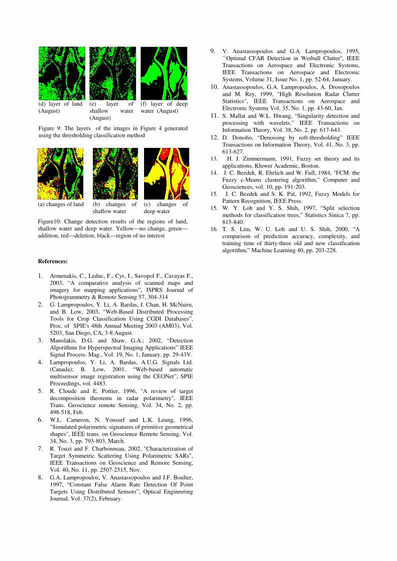
“Layers” can be defined as images containing part of the information of the original image. For example, for a multi-band image, each band can be viewed as a layer. The mean of all the bands can be also viewed as a layer. Applying the Principle Component Analysis (PCA) to the multi-band image, the images generated by the principle components are also the layers of the original image. Another example of layers is applying the orthogonal decomposition to the original image, the resulting orthogonal components are the layers of the image. Saying a set of layers are “complete” means the original image can be fully generated using this set of layers. The layers are generated based on the user’s need. Each layer should contain only part of the information of interested. Normally, compared with the original image, each layer contains less information, so it’s easier to perform the calculations, transformations based on layers. Furthermore, in some cases, only parts of the layers are useful such as in image fusion by PCA. For the topographic change detection, we are interested in the region changes for different time, so the layers we used in this paper are based on the region classifications. Each layer contains only one region of the original image. In Figure 6, each image contains three regions that are land, shallow water and deep water. These regions should be extracted one by one to generate the layers. Figure 9 shows the corresponding layers of both images. The images in red are the layers of the image taken in May, and the layers taken in August are plotted in green. (a) and (d) are the layer-of-land with land represented in red/green. In (b) and (e), except the regions of shallow water, all the others are in black. So they are the layer-of-shallow water. Similarly, (c) and (f) are the layers-of-deep water.

,)()1()()1( ��=∩ −− ik

ik

ik

ik LLRR �

,)()1()()( �−�= − ik

ik

ik

ik LLLA �

.2 )1()()1()()()()( �−+�=+= −− ik

ik

ik

ik

ik

ik

ik LLLLDAC �

.)()1()1()( �−�= −− ik

ik

ik

ik LLLD �

,)()1()()1( ��=∩ −− ik

ik

ik

ik LLRR �

.')()( ii CC =

4. TOPOGRAPHIC CHANGE DETECTION

4.1 Change Detection Based on Region Classification

Topographic change detection is studying changes on the surface of the earth. Satellite images are used to perform topographic detection at very high accuracy. In this paper we present a topographic change detection method that applies the automatic update algorithm presented in [1]. Namely, for a two level classification problem we consider an image � = S1 + S2, where Si, i=1,2 are compact regions of the image represented by contours. The contours enclose pixels that correspond to the same region. When a change occurs, two groups of pixels are changing region. Those that move from region S1 to region S2 are named as “additions” (A), while the others that change from region S2 to region S1 are called “deletions” (D). The total change C in the image I is expressed as the summation of additions and deletions, C=A+D. Namely,

(1)

where the subscript “i” and “i-1” are the time index, which represent the current and previous time, respectively. The advantage of this method is details of the changes are provided. In a log of applications, we are not only interested in where the changes happen, but also how are the changes. In the following, we will extend this concept to multiple region cases and automatic update of information. In a distributed processing system this mechanism may be programmed to keep updates of changes of classification regions or other features over time. For the images have multiple level classification, we are interested in the changes in each region, i.e. addition and deletion. Assume we have M interested regions, which are presented in M “layers”, ,,,, 21 MLLL � where the region-of-

interest in the layer iL is denoted as iR . The pixels in

iR have

values “1” and all the other pixels are set to zeros. The basic idea is comparing the pairs of layers of different times one by

one. Namely, find the addition and deletion for each iL . For

each pair of layers, the region-of-interestiR is exactly the

2S in

our previous discussion, and the other part having zero values is the

1S . In this way, if we use )(ikL to denote the kth layer at time

I, the common region of interest will be

(2)

where the operator “� ” represents the element-by-element

multiplication of two matrices, and “ ��* ” represents a region which is composed of the pixels whose values are ones in “*”. In this way, the addition of

kR therefore will be (3)

and the deletions is (4)

The total change for the k th region will be

(5)

However, if we perform frame-to-frame subtraction, we will obtain

(6)

and we have (7)

From the above we can see in a two level classification problem the total change may be expressed through the absolute value of a frame-to-frame differencing. In practice we are interested in more details of the changes such as additions and deletions. Our proposed formulations give these details. Apply the above procedures to each pair of layers. Step by step the addition and deletion for every class will be detected sequentially. 4.2 Change Detection Based on Pixel Level Characteristics

The ability to preserve the pixel characteristics from frame to frame when change detection is performed is essential if multiple classification inferences are derived from the changes. In this case image classification process is carried out on the change detection results. Two methods have been studied for change detection on images with multiple classification regions, i.e. the principal component analysis and the wavelet method. 4.3 Matched filtering and change detection.

Change detection may be applied using matched filters. Matched filters tend to suppress clutter and emphasize the changes of interest. When matched filters are applied the change detection performance increases. Matched filtering for change detection is normally applied to multispectra and/or multipolarized images [3], [5]-[7]. 5. EXAMPLE

Let’s consider the two images in Figure 4. Their layers are presented in Figure 9. We apply the proposed multi-level change detection method to the pair of layers {(a), (d)}, {(b), (e)} and {(c), (f)}, respectively. The result is displayed in Figure 10, where the red regions represent deletions, green ones stand for additions, and the yellow means no change happens. Figure 10 clearly gives the details of change in each region. It is easy to find from Figure 10 (c), because of the flooding in May, some regions of shallow water and land in the image of August become deep water (the red region in (c)). For the same reason, in (a), the green regions are the parts that are changed from shallow and deep water in May to land in August. Using this method avoids need for strict radiometric calibration. We can choose the appropriate classification scheme. The most important is it designates the types of changes occurring. It is simple, reliable and effective.

)(1

)1(1

)1(1

)(

)(1

)1(1

)(1

)(

)1(2

)1(1

)1(

)(2

)(1

)(

iiii

iiii

iii

iii

SSSA

SSSD

SSI

SSI

∩−=

∩−=

+=

+=

−−

−

−−−

May August Figure 3: Two level region classification results using thresholding method. The black areas represent water.

May August Figure 4: Two level region classification results using FCM method. The black areas represent water.

May August Figure 5: Two level region classification results using decision tree method. The black areas represent water. 6. CONCLUSION In this paper, several classification methods are first presented and the results are compared. We then introduce the definition of “layer” and how to create it. Based on the “layer”, a multiple level change detection algorithm is proposed, which gives the details of the changes in each region and is demonstrated to be an easy, effective and reliable method. Experimental results are provided using RADARSAT images.

May August Figure 6: Three level region classification results using thresholding method.

May August Figure 7: Three level region classification results using FCM method.

May August Figure 8: Three level region classification results using the decision tree method.

(a) layer of land

(May) (b) layer of shallow water (May)

(c) layer of deep water (May)

(d) layer of land (August)

(e) layer of shallow water (August)

(f) layer of deep water (August)

Figure 9: The layers of the images in Figure 4 generated using the thresholding classification method

(a) changes of land (b) changes of

shallow water (c) changes of deep water

Figure10: Change detection results of the regions of land, shallow water and deep water. Yellow—no change, green—addition, red—deletion, black—region of no interest

References: 1. Armenakis, C., Leduc, F., Cyr, I., Savopol F., Cavayas F.,

2003, “A comparative analysis of scanned maps and imagery for mapping applications”, ISPRS Journal of Photogrammetry & Remote Sensing 57, 304-314

2. G. Lampropoulos, Y. Li, A. Bardas, J. Chan, H. McNairn, and B. Low, 2003, “Web-Based Distributed Processing Tools for Crop Classification Using CGDI Databases”, Proc. of SPIE's 48th Annual Meeting 2003 (AM03), Vol. 5203, San Diego, CA, 3-8 August.

3. Manolakis, D.G. and Shaw, G.A.; 2002, “Detection Algorithms for Hyperspectral Imaging Applications” IEEE Signal Process. Mag., Vol. 19, No. 1, January, pp. 29-43V.

4. Lampropoulos, Y. Li, A. Bardas, A.U.G. Signals Ltd. (Canada); B. Low, 2001, “Web-based automatic multisensor image registration using the CEONet”, SPIE Proceedings, vol. 4483.

5. R. Cloude and E. Pottier, 1996, "A review of target decomposition theorems in radar polarimetry", IEEE Trans. Geoscience remote Sensing, Vol. 34, No. 2, pp. 498-518, Feb.

6. W.L. Cameron, N. Youssef and L.K. Leung, 1996, "Simulated polarimetric signatures of primitive geometrical shapes", IEEE trans. on Geoscience Remote Sensing, Vol. 34, No. 3, pp. 793-803, March.

7. R. Touzi and F. Charbonneau, 2002, "Characterization of Target Symmetric Scattering Using Polarimetric SARs", IEEE Transactions on Geoscience and Remore Sensing, Vol. 40, No. 11, pp. 2507-2515, Nov.

8. G.A. Lampropoulos, V. Anastassopoulos and J.F. Boulter, 1997, “Constant False Alarm Rate Detection Of Point Targets Using Distributed Sensors”, Optical Engineering Journal, Vol. 37(2), February.

9. V. Anastassopoulos and G.A. Lampropoulos, 1995, ``Optimal CFAR Detection in Weibull Clutter'', IEEE Transactions on Aerospace and Electronic Systems, IEEE Transactions on Aerospace and Electronic Systems, Volume 31, Issue No. 1, pp. 52-64, January.

10. Anastassopoulos, G.A. Lampropoulos, A. Drosopoulos and M. Rey, 1999, "High Resolution Radar Clutter Statistics", IEEE Transactions on Aerospace and Electronic Systems Vol. 35, No. 1, pp. 43-60, Jan.

11. S. Mallat and W.L. Hwang, “Singularity detection and processing with wavelets.” IEEE Transactions on Information Theory, Vol. 38, No. 2, pp. 617-643.

12. D. Donoho, “Denoising by soft-thresholding” IEEE Transactions on Information Theory, Vol. 41, No. 3, pp. 613-627.

13. H. J. Zimmermann, 1991, Fuzzy set theory and its applications, Kluwer Academic, Boston.

14. J. C. Bezdek, R. Ehrlich and W. Full, 1984, "FCM: the Fuzzy c-Means clustering algorithm," Computer and Geosciences, vol. 10, pp. 191-203.

15. J. C. Bezdek and S. K. Pal, 1992, Fuzzy Models for Pattern Recognition, IEEE Press.

15. W. Y. Loh and Y. S. Shih, 1997, “Split selection methods for classification trees,” Statistics Sinica 7, pp. 815-840.

16. T. S. Lim, W. U. Loh and U. S. Shih, 2000, “A comparison of prediction accuracy, complexity, and training time of thirty-three old and new classification algorithm,” Machine Learning 40, pp. 203-228.