A Robust and Easy to Implement Method for IMU Calibration withoutExternal Equipments

David Tedaldi, Alberto Pretto and Emanuele Menegatti

Abstract— Motion sensors as inertial measurement units(IMU) are widely used in robotics, for instance in the navigationand mapping tasks. Nowadays, many low cost micro electromechanical systems (MEMS) based IMU are available off theshelf, while smartphones and similar devices are almost alwaysequipped with low-cost embedded IMU sensors. Nevertheless,low cost IMUs are affected by systematic error given byimprecise scaling factors and axes misalignments that decreaseaccuracy in the position and attitudes estimation.In this paper, we propose a robust and easy to implementmethod to calibrate an IMU without any external equipment.The procedure is based on a multi-position scheme, providingscale and misalignments factors for both the accelerometersand gyroscopes triads, while estimating the sensor biases. Ourmethod only requires the sensor to be moved by hand andplaced in a set of different, static positions (attitudes). Wedescribe a robust and quick calibration protocol that exploitsan effective parameterless static filter to reliably detect the staticintervals in the sensor measurements, where we assume localstability of the gravity’s magnitude and stable temperature.We first calibrate the accelerometers triad taking measurementsamples in the static intervals. We then exploit these resultsto calibrate the gyroscopes, employing a robust numericalintegration technique.The performances of the proposed calibration technique hasbeen successfully evaluated via extensive simulations and realexperiments with a commercial IMU provided with a calibra-tion certificate as reference data.

I. INTRODUCTION

IMUs (Inertial Measurement Units) are very popularsensors in robotics: among others, they have been exploitedfor inertial-only navigation [1], attitude estimation [2], andvisual-inertial navigation [3], [4], also using a smartphonedevice [5]. IMUs used in robotics are usually based onMEMS (micro electro mechanical systems) technology.They are composed by a set of tri-axial clusters: anaccelerometers, a gyros and often a magnetometer cluster.In an ideal IMU, the tri-axial clusters should share the same3D orthogonal sensitivity axes that span a three dimensionalspace, while the scale factor should convert the digitalquantity measured by each sensor into the real physicalquantity (e.g, accelerations and gyro rates). Unfortunately,low cost MEMS based IMU are usually affected by nonaccurate scaling, sensor axis misalignments, cross-axis

This research has been partially supported by Consorzio Ethics withthe grant ”Rehabilitation Robotics”, by Univ. of Padova with the grant“TIDY-UP: Enhanced Visual Exploration for Robot Navigation and Ob-ject Recognition”, and by the European Commission under FP7-600890-ROVINA. The authors are with the Department of Information Engineering,University of Padova, Italy. Email: david.tedaldi@gmail.com,emg@dei.unipd.it. Pretto is also with the Department of Computer,Control, and Management Engineering “Antonio Ruberti“, Sapienza Univer-sity of Rome, Italy. Email: pretto@dis.uniroma1.it

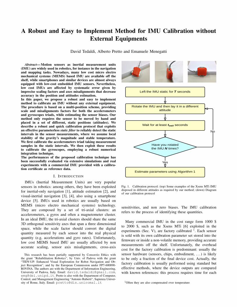
Fig. 1. Calibration protocol: (top) Some examples of the Xsens MTi IMUdisposed in different attitudes as required by our method; (down) Diagramof our calibration protocol

sensitivities, and non zero biases. The IMU calibrationrefers to the process of identifying these quantities.

Many commercial IMU in the cost range form 1000 $to 2000 $, such as the Xsens MTi [6] exploited in theexperiments (Sec. V), are factory calibrated 1. Each sensoris sold with its own calibration parameter set stored into thefirmware or inside a non-volatile memory, providing accuratemeasurements off the shelf. Unfortunately, the overheadcost for the factory calibration is predominant: usually thesensor hardware (sensors, chips, embodiment, . . . ) is likelyto be only a fraction of the final device cost. Actually, thefactory calibration is usually performed using standard buteffective methods, where the device outputs are comparedwith known references: this process requires time for each

1Often they are also compensated over temperature

sensor and a high cost equipment. On the other hand, low-cost IMUs (20-100 $) and the IMU sensors that equip currentsmartphones are usually poorly calibrated, resulting in mea-surements coupled with not negligible systematic errors. Forinstance, state-of-the-art visual-inertial navigation systemssuch the one presented in [5], that exploits a smartphone asexperimental platform, while performing so well in forward,almost regular, motion 2, shows lower performances in more“exciting” motions, i.e. in motions that quickly change linearacceleration and rotational axes.In this paper, we propose an effective and easy to imple-ment calibration scheme, that only requires to collect IMUdata with the simple procedure described in the flow chartreported in Fig. 1. After an initial initialization period withno motion, the operator should move the IMU in differentpositions, in order to generate a set of distinct, temporarilystable, rotations. The collected dataset is used to calibrate thescale and misalignments factors for both the accelerometersand gyroscopes triads, while estimating the sensor biases.As other calibration technique, we neglect the effect of thecross-axis sensitivities, since for minor misalignments andminor cross-axis sensitivities errors it is usually difficult todistinguish between them.Our procedure exploits the basic idea of the multi-positionmethod, firstly presented in [7] for accelerometers calibra-tion: in a static position, the norms of the measured acceler-ations is equal to the magnitudes of the gravity plus a multi-source error factor (i.e., it includes biases, misalignment,noise,...). All these quantities can be estimated via minimiza-tion over a set of static attitudes. After the calibration of theaccelerometer triad, we can use the gravity vector positionsmeasured by the accelerometers as a reference to calibrate thegyroscope triad. Integrating the angular velocities betweentwo consecutive static positions, we can estimate the gravitypositions in the new orientation. The gyroscopes calibrationis finally obtained minimizing the errors between theseestimates and the gravity references given by the calibratedaccelerometers.In this procedure the gyroscopes calibration accuracystrongly depends on the accuracy of the accelerometers cali-bration, being used as a reference. Moreover, signal noise andbiases should negatively affect both the calibration accuracyand the reliability of the algorithms used to detect the actualstatic intervals used in the calibration. Finally, a consistentnumerical integration process is essential to mitigate theeffect of the signal discretization, usually sampled at 100Hz. In our approach, we face these problems introducingthe following modifications to the standard multi-positionmethod:

• The proposed calibration protocol exploits a largernumber of static states with reduced periods, in order toincrease the cardinality of the dataset while preservingthe assumption of local stability of the sensors biases

• As proposed in [8], we characterize the gyroscope bias

2Actually, during an almost regular motion miscalibration errors mayeasily be assimilated by the biases included in the system state

drifts in a period estimated using the Allan variance• We introduce a simple but effective static detector

that exploits the sensor noise magnitude, a fixed-timesampling window and a cutting threshold, automaticallyestimated inside the optimization framework

• We employ the Runge-Kutta numerical integrationmethod to improve the accuracy of the gyroscope cali-bration.

We have extensively tested our system using synthetic dataaffected by variable biases, misalignments, scale factor er-rors, and noise. In all of the cases, we have obtainedstable and accurate results. Moreover, we have performedthe calibration of a commercial, factory calibrated XsensMTi IMU, using its raw, uncalibrated data as input. Ourcalibration results are comparable to the factory parametersreported by the device’s calibration certificate.

A. Related Works

Traditionally the calibration of an IMU has been done byusing special mechanical platforms such as a robotic ma-nipulator, moving the IMU with known rotational velocitiesin a set of precisely controlled orientations [9], [10], [11].At each orientation, the output of the accelerometers arecompared with the precomputed gravity vector while duringthe rotations the output of gyroscopes are compared with theprecomputed rotational velocity. However, the mechanicalplatforms used for calibration are usually very expensive,resulting in a calibration cost that often exceeds the cost ofthe IMU’s hardware.In [12] a calibration procedure that exploits a marker-based optical tracking system has been presented, while in[13], the GPS readings are used to calibrate initial biasesand misalignments. Clearly, the accuracy of these methodsstrongly depends on the accuracy of the employed kinematicreference (i.e., the motion capture system or the GPS). Themulti-position method was firstly introduced by Lotters et al.[7]: they proposed to calibrate the biases and the scale factorof the accelerometers using the fact that the magnitude ofthe static acceleration must equal to the gravity’s magnitude.This technique has been extended in [14] and [15] to includethe accelerometer axis misalignment. The error model theyproposed for the gyroscopes is similar to the one used forthe accelerometers, but the calibration procedure in thiscase requires a single axis turntable to provide a strongrotation rate signal, providing high calibration accuracy. Un-fortunately, these approaches not only require a mechanicalequipment, but the two triads are independently calibrated,and the misalignment between them can’t be detected. In[8] and [16] authors presented two calibration schemes thatdo not require any external mechanical equipment. Similarlyto our approach, in the first work the authors calibratethe accelerometers exploiting the high local stability of thegravity vector’s magnitude, and then gyroscopes calibrationis obtained comparing the gravity vector sensed by thecalibrated accelerometer with the gravity vector obtained byintegrating the angular velocities. In the second work theauthors also exploit the local stability of the magnetic field.

Hwangbo et al. [17] recently proposed a self-calibrationtechnique based on an iterative matrix factorization. Theyuse gravity as accelerometers reference, and a camera asgyroscopes reference.

II. SENSOR ERROR MODEL

For an ideal IMU, the 3 axes of the accelerometerstriad and the 3 axes of the gyroscopes triad define asingle, shared, orthogonal 3D frame. Each accelerometersenses the acceleration along of one distinct axis, whileeach gyroscope measures the angular velocity around thesame axis. Unfortunately in real IMUs, due to assemblyinaccuracy, the two triads form two distinct (i.e., misaligned),non-orthogonal, frames. Also the single sensors are notperfect: typically the scaling factors used to convert thedigital outputs of the sensors in real physical quantityare different for different instances of the same sensors,while only a default, nominal scaling factor is providedby manufacturers. Moreover, the output signals are almostalways affected by non zero, variable biases.

As introduced above, both the accelerometers frame (AF)and the gyroscopes frame (GF) are usually non-orthogonal.We can define two associated orthogonal, ideal frames (AOFand GOF, respectively) in the following way:

• The x-axis of the AOF and the one of the AF coincide• The y-axis of the AOF lies in the plan spanned by the

x and y axes of the AF.For the gyroscopes case, it is sufficient to substitute the AFand AOF acronyms with GF and GOF, respectively. Finally,we define a body frame (BF), which is an orthogonal framethat represents, for example, the coordinate frame of theIMU’s chassis. The body frame usually differs from theAF and GF frames by small angles but, in general, thereis no direct relation between them. For small angles, ameasurement sS in a non-orthogonal frame (AF or GF) canbe transformed in the orthogonal body frame as (for detailsof the derivation, see [18]):

sB = TsS , T =

1 −βyz βzyβxz 1 −βzx−βxy βyx 1

(1)

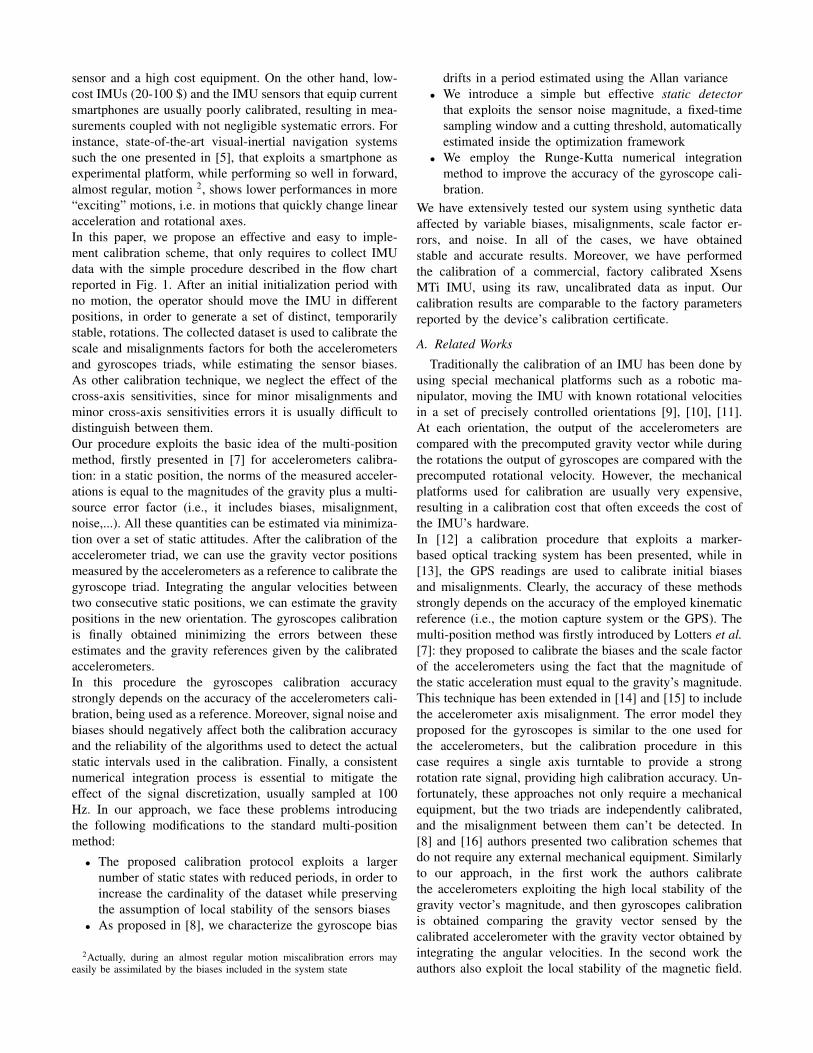
where sB and sS denote the specific force (acceleration),or equivalently the rotational velocity, in the body framecoordinates and accelerometers (or gyroscopes) coordinates,respectively. Here βij is the rotation of the i-th accelerometeror gyroscope axis around the j-th BF axis, see Fig. 2.

On the other hand, the two orthogonal frames BF andAOF (and, equivalently, BF and GOF) are relate by a purerotation.In the presented calibration method, we assume that thebody frame BF coincides with the accelerometers orthogonalframe AOF: in such case, the angles βxz, βxy, βyx becomezero, so in the accelerometers case Eq. 1 becomes:

aO = TaaS , Ta =

1 −αyz αzy

0 1 −αzx

0 0 1

(2)

Fig. 2. Non-orthogonal sensor (accelerometers or gyroscopes) axes (xS ,yS , zS ), and body frame axes (xB , yB , zB).

where we have changed letter β, referring to the generalcase, with the letter α, referring to the accelerometer case,while aO and aS denote the specific acceleration in AOFand AF, respectively3.

As mentioned before, gyroscope and accelerometer mea-surements should refer to the same reference frame, in ourcase AOF. Then, using Eq. 1, for the gyroscopes, we have:

ωO = TgωS , Tg =

1 −γyz γzyγxz 1 −γzx−γxy γyx 1

(3)

where ωO and ωS denote the specific angular velocities inAOF and in GF , respectively.

Both the accelerometers and the gyroscopes are affectedby biases and scale errors. Two scaling matrix are introduced

Ka =

sax 0 00 say 00 0 saz

, Kg =

sgx 0 00 sgy 00 0 sgz

(4)

We introduce also two bias vector

ba =

baxbaybaz

, bg =

bgxbgybgz

(5)

The complete sensor error model is

aO = TaKa(aS + ba + νa) (6)

for the accelerometers, and

ωO = TgKg(ωS + bg + νg) (7)

for the gyroscope, where νg and νg are the accelerometermeasurement noise and the gyroscope measurement noise,respectively.

3To relate the obtained calibration with a different body frame (e.g.BF’), it is sufficient to estimate the rotation matrix that relate AOF to BF’,for instance using the accelerometers outputs in three different orthogonalorientations.

III. BASIC CALIBRATION FRAMEWORK

In order to calibrate the accelerometers triad, we need toestimate the following unknown parameter vector:

θacc =[αyz, αzy, αzx, s

ax, s

ay, s

az , b

ax, b

ay, b

az

](8)

We define the following function:

aO = h(aS ,θacc) = TaKa(aS + ba) (9)

Here we can neglect the measurements noise thanks tothe fact that in our calibration procedure we apply signalaveraging in each static interval.As in the conventional multi-position scheme, we move theIMU in a set of M distinct, temporarily stable, rotations.We can extract M acceleration vectors aS

k (measured in thenon-orthogonal AF), averaging the accelerometers readingsin a temporal window inside each static interval. The costfunction we use to estimate accelerometers’ parameters is:

L(θacc) =M∑k=1

(||g||2 − ||h(aSk ,θ

acc)||2)2 (10)

where ||g|| is the actual magnitude of the local gravityvector that can easily recovered from specific public tables(e.g., knowing latitude, longitude and altitude of the locationwhere we are performing the calibration). In order tominimize Eq. 10, we employ the Levenberg-Marquardt(LM) algorithm.

In order to calibrate the gyroscope triad, we can assumethe system as bias-free simply averaging the static gyroscopesignals over a suitable initial period of no motion. Thisis justified by the following discussion about the Allanvariance (see Sec. IV-C). Moreover, since we need to use theaccelerometers as known references, we use the calibrationparameters θacc computed above, correcting the accelerom-eters readings with Eq. 9.We define the operator Ψ, that takes as input a sequence of ngyroscopes readings ωS

i and an initial gravity versor ua,k−1

(i.e., a unit vector representing the gravity direction) givenby the calibrated accelerometers, and return the final gravityversor ug,k, computed using the gyroscopes measurementsbetween the k − 1-th and the k-th static intervals:

ug,k = Ψ[ωSi ,ua,k−1

](11)

Ψ can be any integration algorithm that computes the finalorientation through integrating the input angular velocities.The unknown parameter vector we need to estimate tocalibrate the gyroscope is:

θgyro =[γyz, γzy, γxz, γzx, γxy, γyx, s

gx, s

gy, s

gz

](12)

In this case, we can define the cost function as:

L(θgyro) =

M∑k=2

||ua,k − ug,k||2 (13)

where M is the number of static intervals, ua,k is the accel-eration versor measured averaging in a temporal window the

calibrated accelerometer readings in the k-th static interval,and ug,k is the acceleration versor computed using Eq. 11(i.e., integrating the angular velocities between the k− 1-thand the k-th static intervals). We obtain θgyro minimizingEq. 13 with LM.

IV. CALIBRATION PROCEDURE

As introduced in Sec. I, the proposed calibration frame-work requires to collect a dataset with the stream of theraw accelerometers and gyroscopes readings, taken while theoperator moves the IMU in different static positions, in orderto generate a set of distinct, temporarily stable, rotations.A simple diagram of our calibration protocol is reported inFig. 1. As mentioned in Sec. III, to mitigate the noise effectin the minimization of Eq. 10 and Eq. 13, we need to averagethe signals over a suitable time interval. This imposes a lowerbound in the length of the static interval (twait in Fig. 1).A initialization period (Tinit in Fig. 1) with no motion isessential as well: this will be exploited to characterize thegyroscopes biases (Sec. IV-C) and the static detector operator(Sec. IV-A).

A. Static Detector

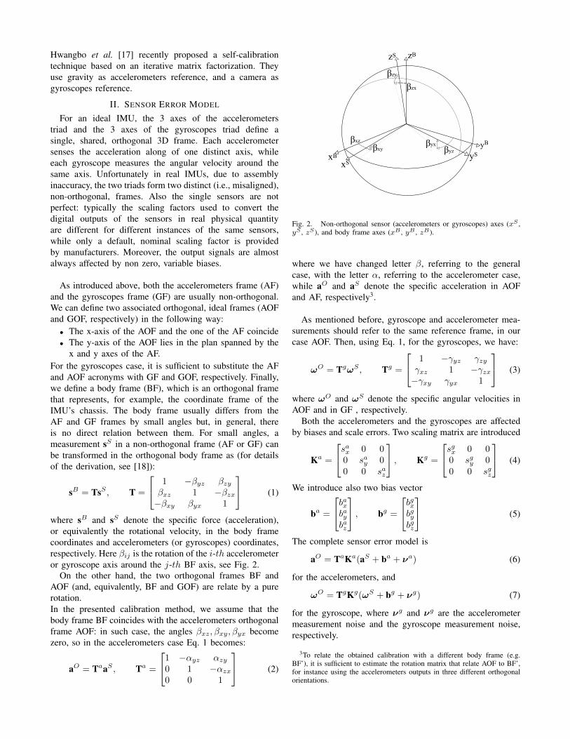
Fig. 3. An example of the static detector applied to the accelerometersdata: the static detector is represented by the black square wave, its highlevel classify an interval as static.

The accuracy of the calibration strongly depends on thereliability in the classification between static and motionintervals: to calibrate the accelerometers we use static inter-vals, while for gyroscopes calibration we also include themotion intervals between two consecutive static intervals.In our experience, band-pass filter based operators, like thequasi-static detector used in [8], perform poorly with realdatasets: detected static intervals frequently includes somesmall portion of motion. Moreover, they require a fine tuning,since they depend on three parameters.We propose instead to use a variance based static detectoroperator, that exploits the lower bound in the lengths of thestatic interval introduced above. We base our detector onthe accelerometer signals: given a time interval of lengthtwait seconds (see Fig. 1), for each accelerometers sample(at

x, aty, at

z) at time t, we compute the variance magnitude,i.e. the magnitude of the variance, as:

ς(t) =√

[vartw(atx)]2 + [vartw(aty)]2 + [vartw(atz)]2 (14)

where vartw(at) is an operator that compute the variance ofa general signal at in a time interval of length tw secondscentered in t. We classify between static and motion intervalssimply checking if the square of ς(t) is lower or greater thena threshold. As a threshold, we consider an integer multipleof the square of the variance magnitude ςinit, computed overall the initialization period Tinit. In all the experiments, weuse tw = 2 sec, while Tinit is estimated using the Allanvariance (see Sec. IV-C). It is important to note that ourstatic detector does not require any parameter tuning: theinteger multiplier used in the classification is automaticallyestimated by our calibration algorithm (see Sec. IV-D). Fig. 3reports an example of how our static filter works on real data:in this case the estimated integer multiplier is 6.

B. Runge-Kutta IntegrationAs reported in Eq. 11, in the gyroscopes calibration we

need to perform a discrete time angular velocity integration:a robust and stable numerical integration method is desir-able since it can improve the calibration accuracy. Givena common instruments rate of 100 Hz (like the XsensMTi IMU used in the experiments) and since we representrotations using quaternion arithmetic, with this setup a properintegration algorithm choice [19] is the Runge-Kutta 4th

order normalized method (RK4n). In our experience (experi-ments not reported for space constraints) RK4n outperformsthe standard linear integration procedure providing higheraccuracy results. Let Eq. 15 be the differential equationdescribing the quaternion kinematics:

f(q, t) = q =1

2Ω(ω(t))q, (15)

where Ω(ω) is the operator which turns the considered tri-dimensional angular velocity into the real skew symmetricmatrix representation, that is:

Ω(ω) =

0 −ωx −ωy −ωz

ωx 0 ωz −ωy

ωy −ωz 0 ωx

ωz ωy −ωx 0

. (16)

The RK4n integration algorithm is:

qk+1 = qk + ∆t1

6(k1 + 2k2 + 2k3 + k4) , (17)

ki = f(q(i), tk + ci∆t), (18)q(i) = qk, for i = 1, (19)

q(i) = qk + ∆t

i−1∑j=1

aijkj , for i > 1. (20)

where all the coefficients needed, ci and aij , are

c1 = 0, c2 = 12 , c3 = 1

2 , c4 = 1,

a21 = 12 , a31 = 0, a41 = 0,

a32 = 12 , a42 = 0, a43 = 1.

Finally, for each step, we also need to normalize the (k+1)-th quaternion:

qk+1 →qk+1

||qk+1||. (21)

C. Allan Variance

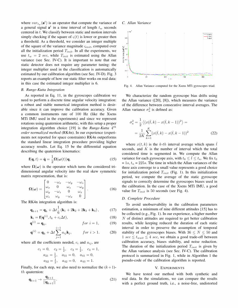
Fig. 4. Allan Variance computed for the Xsens MTi gyroscopes triad.

We characterize the random gyroscope bias drifts usingthe Allan variance ([20], [8]), which measures the varianceof the difference between consecutive interval averages. TheAllan variance σ2

a is defined as:

σ2a =

1

2

⟨(x(t, k)− x(t, k − 1))2

⟩=

=1

2K

K∑k=1

(x(t, k)− x(t, k − 1))2 (22)

where x(t, k) is the k-th interval average which spans tseconds, and K is the number of interval which the totalconsidered time is segmented in. We compute the Allanvariance for each gyroscope axis, with t0 ≤ t ≤ tn. We fix t0= 1s, tn = 225s. The time in which the Allan variances of thethree axis converge to a small value represents a good choicefor initialization period Tinit (Fig. 1). In this initializationperiod, we compute the average of the static gyroscopesignals to correctly determine the gyroscopes biases used inthe calibration. In the case of the Xsens MTi IMU, a goodvalue for Tinit is 50 seconds (see Fig. 4).

D. Complete Procedure

To avoid unobservability in the calibration parametersestimation, a minimum of nine different attitudes [15] has tobe collected (e.g., Fig. 1). In our experience, a higher numberN of distinct attitudes are required to get better calibrationresults, while keeping reduced the duration of each staticinterval in order to preserve the assumption of temporalstability of the gyroscopes biases. With 36 ≤ N ≤ 50 and1 sec ≤ twait ≤ 4 sec, we obtain a good trade-off betweencalibration accuracy, biases stability, and noise reduction.The duration of the initialization period Tinit is given bythe Allan variance analysis (see Sec. IV-C). The calibrationprotocol is summarized in Fig. 1, while in Algorithm 1 thepseudo-code of the calibration algorithm is reported.

V. EXPERIMENTS

We have tested our method with both synthetic andreal data. In the simulations, we can compare the resultswith a perfect ground truth, i.e., a noise-free, undistorted

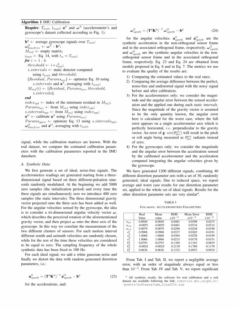
Algorithm 1 IMU CalibrationRequire: Tinit, twait; aS and ωS (accelerometer’s andgyroscope’s dataset collected according to Fig. 1).

bg ← average gyroscope signals over Tinit;ωS

biasfree ← ωS - bg;Minf ← empty matrix;ςinit ← Eq. 14, with tw = Tinit;for i = 1 : kthreshold ← i ∗ ς2init;s intervals ← static detector computed

using twait and threshold;[Residual, Paramsacc] ← optimize Eq. 10 usings intervals and aS , averaging with twait;

Minf (i) ← [Residual, Paramsacc, threshold,s intervals];

endindexopt ← index of the minimum residual in Minf ;Paramsacc ← from Minf using indexopt;s intervalsopt ← from Minf using indexopt;aO ← calibrate aS using Paramsacc;Paramsgyro ← optimize Eq. 13 using s intervalsopt,ωS

biasfree and aO, averaging with twait.

signal, while the calibration matrices are known. With thereal dataset, we compare the estimated calibration param-eters with the calibration parameters reported in the IMUdatasheet.

A. Synthetic Data

We first generate a set of ideal, noise-free signals. Theaccelerometers readings are generated starting from a three-dimensional signal based on three different-pulsation sinu-soids randomly modulated. At the beginning we add 5000zero samples (the initialization period) and every time thethree signals are simultaneously zero we introduce 400 zerosamples (the static intervals). The three dimensional gravityvector projected onto the three axis has been added as well.For the angular velocities sensed by the gyroscope, the ideais to consider a tri-dimensional angular velocity vector ω,which describes the perceived rotation of the aforementionedgravity vector, and then project ω onto the three axis of thegyroscope. In this way we correlate the measurement of thetwo different clusters of sensors. For each motion intervaldifferent zenith and azimuth velocities are randomly chosen,while for the rest of the time these velocities are consideredto be equal to zero. The sampling frequency of the wholesynthetic data has been fixed to 100 Hz.

For each ideal signal, we add a white gaussian noise andfinally we distort the data with random generated distortionparameters, i.e.:

aSsynth = (TaKa)

−1 aOsynth − ba (23)

for the accelerations, and:

ωSsynth = (TgKg)

−1ωO

synth − bg (24)

for the angular velocities. aSsynth and aOsynth are thesynthetic acceleration in the non-orthogonal sensor frameand in the associated orthogonal frame, respectively. ωS

synth

and ωOsynth are the synthetic angular velocities in the non-

orthogonal sensor frame and in the associated orthogonalframe, respectively. Eq. 23 and Eq. 24 are obtained frommodels proposed in Eq. 6 and in Eq. 7. The metrics we useto evaluate the quality of the results are:

1) Comparing the estimated values to the real ones;2) Comparing the average difference between the perfect,

noise-free and undistorted signal with the noisy signalbefore and after calibration;

3) For the accelerometers only: we consider the magni-tude and the angular error between the sensed acceler-ation and the applied one during each static intervals.Since the magnitude of the gravity vector is assumedto be the only quantity known, the angular errorhere is calculated for the worst case, where the fullerror appears on a single accelerometer axis which isperfectly horizontal, i.e. perpendicular to the gravityvector. An error of g ·sin(θaccdiv ) will result in the pitchor roll angle being measured as θaccdiv radiants insteadof zero;

4) For the gyroscopes only: we consider the magnitudeand the angular error between the acceleration sensedby the calibrated accelerometer and the accelerationcomputed integrating the angular velocities given bythe gyroscope.

We have generated 1200 different signals, combining 40different distortion parameter sets with a set of 30, randomlygenerated, ideal signals. Due to reduced space, we reportaverage and worst case results for one distortion parameterset, applied to the whole set of ideal signals. Results for theother distortion parameter sets are very similar4.

TABLE IFirst metric: ACCELEROMETERS PARAMETERS

Real Mean RMS Mean Error RMSValue value x10−3 x10−3 x10−3

αyz 0.0049 0.0049 0.0481 0.0398 0.0275αzy -0.0055 -0.0055 0.0401 0.0334 0.0214αzx 0.0079 0.0079 0.0296 0.0248 0.0190sax 0.9908 0.9908 0.0327 0.0265 0.0191say 1.0068 1.0068 0.0304 0.0258 0.0199saz 1.0066 1.0066 0.0215 0.0178 0.0151bax 0.0793 0.0793 0.1369 0.1163 0.0819bay -0.0024 -0.0024 0.2138 0.1760 0.1178baz 0.0636 0.0636 0.1332 0.0953 0.0919

From Tab. I and Tab. II, we report a negligible averageerror, with an order of magnitude always equal or lessthan 10−4. From Tab. IV and Tab. V, we report significant

4 All synthetic results, the software for real calibration and a realdataset are available following the link: robotics.dei.unipd.it/˜pretto/software/tpm_icra2014.zip

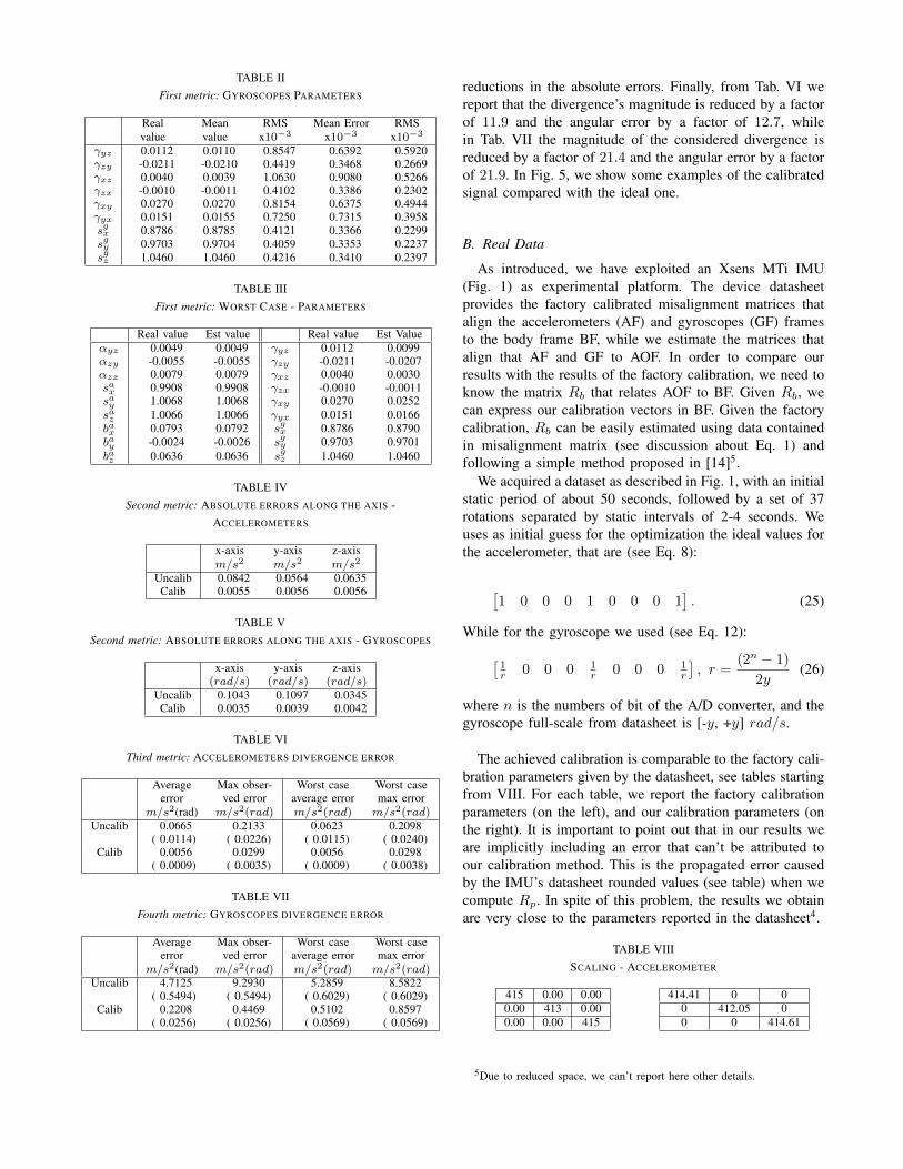
TABLE IIFirst metric: GYROSCOPES PARAMETERS

Real Mean RMS Mean Error RMSvalue value x10−3 x10−3 x10−3

γyz 0.0112 0.0110 0.8547 0.6392 0.5920γzy -0.0211 -0.0210 0.4419 0.3468 0.2669γxz 0.0040 0.0039 1.0630 0.9080 0.5266γzx -0.0010 -0.0011 0.4102 0.3386 0.2302γxy 0.0270 0.0270 0.8154 0.6375 0.4944γyx 0.0151 0.0155 0.7250 0.7315 0.3958sgx 0.8786 0.8785 0.4121 0.3366 0.2299sgy 0.9703 0.9704 0.4059 0.3353 0.2237sgz 1.0460 1.0460 0.4216 0.3410 0.2397

TABLE IIIFirst metric: WORST CASE - PARAMETERS

Real value Est value Real value Est Valueαyz 0.0049 0.0049 γyz 0.0112 0.0099αzy -0.0055 -0.0055 γzy -0.0211 -0.0207αzx 0.0079 0.0079 γxz 0.0040 0.0030sax 0.9908 0.9908 γzx -0.0010 -0.0011say 1.0068 1.0068 γxy 0.0270 0.0252saz 1.0066 1.0066 γyx 0.0151 0.0166bax 0.0793 0.0792 sgx 0.8786 0.8790bay -0.0024 -0.0026 sgy 0.9703 0.9701baz 0.0636 0.0636 sgz 1.0460 1.0460

TABLE IVSecond metric: ABSOLUTE ERRORS ALONG THE AXIS -

ACCELEROMETERS

x-axis y-axis z-axism/s2 m/s2 m/s2

Uncalib 0.0842 0.0564 0.0635Calib 0.0055 0.0056 0.0056

TABLE VSecond metric: ABSOLUTE ERRORS ALONG THE AXIS - GYROSCOPES

x-axis y-axis z-axis(rad/s) (rad/s) (rad/s)

Uncalib 0.1043 0.1097 0.0345Calib 0.0035 0.0039 0.0042

TABLE VIThird metric: ACCELEROMETERS DIVERGENCE ERROR

Average Max obser- Worst case Worst caseerror ved error average error max error

m/s2(rad) m/s2(rad) m/s2(rad) m/s2(rad)Uncalib 0.0665 0.2133 0.0623 0.2098

( 0.0114) ( 0.0226) ( 0.0115) ( 0.0240)Calib 0.0056 0.0299 0.0056 0.0298

( 0.0009) ( 0.0035) ( 0.0009) ( 0.0038)

TABLE VIIFourth metric: GYROSCOPES DIVERGENCE ERROR

Average Max obser- Worst case Worst caseerror ved error average error max error

m/s2(rad) m/s2(rad) m/s2(rad) m/s2(rad)Uncalib 4.7125 9.2930 5.2859 8.5822

( 0.5494) ( 0.5494) ( 0.6029) ( 0.6029)Calib 0.2208 0.4469 0.5102 0.8597

( 0.0256) ( 0.0256) ( 0.0569) ( 0.0569)

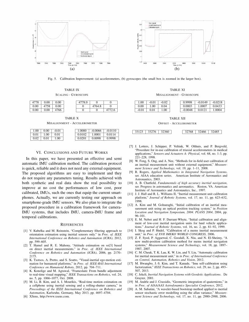
reductions in the absolute errors. Finally, from Tab. VI wereport that the divergence’s magnitude is reduced by a factorof 11.9 and the angular error by a factor of 12.7, whilein Tab. VII the magnitude of the considered divergence isreduced by a factor of 21.4 and the angular error by a factorof 21.9. In Fig. 5, we show some examples of the calibratedsignal compared with the ideal one.

B. Real Data

As introduced, we have exploited an Xsens MTi IMU(Fig. 1) as experimental platform. The device datasheetprovides the factory calibrated misalignment matrices thatalign the accelerometers (AF) and gyroscopes (GF) framesto the body frame BF, while we estimate the matrices thatalign that AF and GF to AOF. In order to compare ourresults with the results of the factory calibration, we need toknow the matrix Rb that relates AOF to BF. Given Rb, wecan express our calibration vectors in BF. Given the factorycalibration, Rb can be easily estimated using data containedin misalignment matrix (see discussion about Eq. 1) andfollowing a simple method proposed in [14]5.

We acquired a dataset as described in Fig. 1, with an initialstatic period of about 50 seconds, followed by a set of 37rotations separated by static intervals of 2-4 seconds. Weuses as initial guess for the optimization the ideal values forthe accelerometer, that are (see Eq. 8):

[1 0 0 0 1 0 0 0 1

]. (25)

While for the gyroscope we used (see Eq. 12):[1r 0 0 0 1

r 0 0 0 1r

], r =

(2n − 1)

2y(26)

where n is the numbers of bit of the A/D converter, and thegyroscope full-scale from datasheet is [-y, +y] rad/s.

The achieved calibration is comparable to the factory cali-bration parameters given by the datasheet, see tables startingfrom VIII. For each table, we report the factory calibrationparameters (on the left), and our calibration parameters (onthe right). It is important to point out that in our results weare implicitly including an error that can’t be attributed toour calibration method. This is the propagated error causedby the IMU’s datasheet rounded values (see table) when wecompute Rp. In spite of this problem, the results we obtainare very close to the parameters reported in the datasheet4.

TABLE VIIISCALING - ACCELEROMETER

415 0.00 0.000.00 413 0.000.00 0.00 415

414.41 0 00 412.05 00 0 414.61

5Due to reduced space, we can’t report here other details.

(a) (b)

Fig. 5. Calibration Improvement: (a) accelerometers, (b) gyroscopes (the small box is zoomed in the larger box).

TABLE IXSCALING - GYROSCOPE

4778 0.00 0.000.00 4758 0.000.00 0.00 4766

4778.0 0 00 4764.8 00 0 4772.6

TABLE XMISALIGNMENT - ACCELEROMETER

1.00 0.00 -0.010.01 1.00 0.010.02 0.01 1.00

1.0000 -0.0066 -0.01100.0102 1.0001 0.01140.0201 0.0098 0.9998

VI. CONCLUSIONS AND FUTURE WORKS

In this paper, we have presented an effective and semiautomatic IMU calibration method. The calibration protocolis quick, reliable and it does not need any external equipment.The proposed algorithms are easy to implement and theydo not require any parameters tuning. Results achieved withboth synthetic and real data show the real possibility toimprove at no cost the performances of low cost, poorcalibrated, IMUs, such the ones that equip the current smart-phones. Actually, we are currently testing our approach onsmartphone-grade IMU sensors. We also plan to integrate theproposed procedure in a calibration framework for camera-IMU systems, that includes IMU, camera-IMU frame andtemporal calibrations.

REFERENCES

[1] V. Kubelka and M. Reinstein, “Complementary filtering approach toorientation estimation using inertial sensors only.” in Proc. of. IEEEInternational Conference on Robotics and Automation (ICRA), 2012,pp. 599–605.

[2] T. Hamel and R. E. Mahony, “Attitude estimation on so[3] basedon direct inertial measurements.” in Proc. of. IEEE InternationalConference on Robotics and Automation (ICRA), 2006, pp. 2170–2175.

[3] K. Tsotsos, A. Pretto, and S. Soatto, “Visual-inertial ego-motion esti-mation for humanoid platforms,” in Proc. of: IEEE-RAS InternationalConference on Humanoid Robots, 2012, pp. 704–711.

[4] K. Konolige and M. Agrawal, “Frameslam: From bundle adjustmentto real-time visual mapping,” IEEE Transactions on Robotics, vol. 24,no. 5, pp. 1066–1077, Oct. 2008.

[5] M. Li, B. Kim, and A. I. Mourikis, “Real-time motion estimation ona cellphone using inertial sensing and a rolling-shutter camera,” inProceedings of the IEEE International Conference on Robotics andAutomation, Karlsruhe, Germany, May 2013, pp. 4697–4704.

[6] XSens, http://www.xsens.com.

TABLE XIMISALIGNMENT - GYROSCOPE

1.00 -0.01 -0.020.00 1.00 0.04-0.01 0.01 1.00

0.9998 -0.0149 -0.02180.0003 1.0007 0.0433-0.0048 0.0121 1.0004

TABLE XIIOFFSET - ACCELEROMETER

33123 33276 32360 32768 32466 32485

[7] J. Lotters, J. Schipper, P. Veltink, W. Olthuis, and P. Bergveld,“Procedure for in-use calibration of triaxial accelerometers in medicalapplications,” Sensors and Actuators A: Physical, vol. 68, no. 1-3, pp.221–228, 1998.

[8] W. Fong, S. Ong, and A. Nee, “Methods for in-field user calibration ofan inertial measurement unit without external equipment,” Measure-ment Science and Technology, vol. 19, pp. 1–11, 2008.

[9] R. Rogers, Applied Mathematics in Integrated Navigation Systems,ser. AIAA education series. American Institute of Aeronautics andAstronautics, 2003.

[10] A. B. Chatfield, Fundamentals of high accuracy inertial navigation,ser. Progress in astronautics and aeronautics. Reston, VA. AmericanInstitute of Aeronautics and Astronautics, Inc., 1997.

[11] J. J. Hall and R. L. Williams II, “Inertial measurement unit calibrationplatform,” Journal of Robotic Systems, vol. 17, no. 11, pp. 623–632,1998.

[12] A. Kim and M. Golnaraghi, “Initial calibration of an inertial mea-surement unit using an optical position tracking system,” in PositionLocation and Navigation Symposium, 2004. PLANS 2004, 2004, pp.96–101.

[13] E. M. Nebot and H. F. Durrant-Whyte, “Initial calibration and align-ment of low-cost inertial navigation units for land vehicle applica-tions.” Journal of Robotic Systems, vol. 16, no. 2, pp. 81–92, 1999.

[14] I. Skog and P. Hndel, “Calibration of a mems inertial measurementunit,” in Proc. of XVII IMEKO WORLD CONGRESS, 2006.

[15] Z. F. Syed, P. Aggarwal, C. Goodall, X. Niu, and N. El-Sheimy, “Anew multi-position calibration method for mems inertial navigationsystems,” Measurement Science and Technology, vol. 18, pp. 1897–1907, 2007.

[16] C. M. Cheuk, T. K. Lau, K. W. Lin, and Y. Liu, “Automatic calibrationfor inertial measurement unit,” in in Proc. of International Conferenceon Control, Automation, Robotics and Vision, 2012.

[17] M. Hwangbo, J.-S. Kim, and T. Kanade, “Imu self-calibration usingfactorization,” IEEE Transactions on Robotics, vol. 29, no. 2, pp. 493–507, 2013.

[18] C. Jekeli, Inertial Navigation Systems with Geodetic Applications. DeGruyter, 2001.

[19] M. Andrle and J. Crassidis, “Geometric integration of quaternions,” inin Proc. of AIAA/AAS Astrodynamics Specialist Conference, 2012.

[20] A. M. Sabatini, “A wavelet-based bootstrap method applied to inertialsensor stochastic error modelling using the allan variance,” Measure-ment Science and Technology, vol. 17, no. 11, pp. 2980–2988, 2006.