a review of computational techniques …dust.ess.uci.edu/ppr/ppr_hun71.pdfa review of computational...

J. Quant. Spectrosc. Radiat. Transfer. Vol. 11, pp. 655~590. Pergamon Press 1971. Printed in Great Britain

A REVIEW OF COMPUTATIONAL TECHNIQUES FOR ANALYSING THE TRANSFER OF RADIATION THROUGH

A MODEL CLOUDY ATMOSPHERE

G. E. HUNT*

Science Research Council, Atlas Computer Laboratory Chilton, Didcot, Berkshire, England

Abstract--We consider the problem of constructing a realistic model cloudy atmosphere. Discussion is made of the computational difficulties associated with computing the single scattering phase diagram which is a problem central to all models. A brief review is made of recent developments in computational techniques for analysing radiative transfer problems. Further discussion is made of various computational economies to reduce computer execution time and storage requirements, and an assessment is made of the penalties paid for implementing these approximations.

1. I N T R O D U C T I O N

ONE OF the fundamental problems of atmospheric physics is concerned with the interpretation of the radiation field emerging from a cloudy atmosphere. The interpretation of the radiometric data will take a different form according to the region of the electromagnetic spectrum at which the measured radiance is centred. In the visible and near infrared spectral regions the problem may be one of determining some of the physical properties of clouds, such as mean particle radius and optical depth from a knowledge of their reflectivities and the degree of polarization of the emergent radiation. In the thermal infrared region, one may be concerned with the derivation of the vertical structure of atmospheric temperature and composition from radiometric measurements of emission from atmospheric gases in their infrared absorption bands. Unfortunately, this type of experiment is greatly hampered by clouds. It is apparent therefore that the common ground of all lower atmosphere radiation studies lies in the problems associated with the radiative properties of clouds. Information regarding such properties obtained in different regions of the spectrum, as well as being of interest in its own right, is fundamental to the interpretation of radiometric measurements.

A convenient method of studying the spectral properties of clouds is from the analysis of characteristics of the radiation scattered by a model cloudy atmosphere. The physical processes which describe the interaction of the radiation field with the cloud particles are well known ~1~ so that the problem of constructing a realistic model of the terrestrial atmosphere is greatly reduced. Models of planetary atmospheres must be simple since at this stage, our knowledge of their physical structure is greatly limited.

*On leave at: Space Sciences Division, Jet Propulsion Laboratory, California Institute of Technology, Pasadena, California 91103.

655

656 G.E. HUNT

In this article we shall review the computational techniques that are at present available to us for the analysis of radiative transfer in a model cloudy atmosphere. We demonstrate that the key relationship in all radiative transfer studies is the interaction principle which expresses the conservation of energy for a finite layer in the atmosphere, t2-4) The application of this exact relationship depends entirely upon the interpretation placed upon the operators involved in it, such as reflection, transmission and source operators.

Central to the construction of these operators is the problem of determining the phase function for a particular model cloud. We shall assume that the scattering particles are dielectric spheres and outline in Section 2 the procedure for determining the phase function. Discussion will be made of the various computational difficulties involved.

The discussion of the computational methods available for theoretical studies of radiative transfer problems given in Section 3 is centred around the formal theory set out by GRANT and HUNT (3) (and in a more abstract manner by PREISENDORFER (2)) which is developed from the interaction principle. The resulting equations may be written either as a differential equation or in a discrete ordinate context, as equivalent matrix equation. As such, this approach defines a more concise way of studying the direct methods that have been developed. Iterative and Monte Carlo methods are studied separately.

To study in detail the radiative properties of realistic and accurately constructed model atmospheres is computationally expensive. In Section 4, we consider various computational economies that may be implemented within model scattering layer and a discussion is made of the penalties paid for using these approximations.

2. COMPUTATIONAL MODELLING

2.1 Interaction principle The type of problem that we shall consider has the simplest geometric configuration,

that of a plane parallel medium, Fig. 1. However, a great deal of the discussion that follows in subsequent sections, may be considered in more general situations, particularly with the ideas of quotient space decomposition exploited by PREISENDORF-ER. (2) But, for the purpose of this review we shall not discuss the implications of the last observation.

In a plane parallel atmosphere, the physical properties depend upon a single space co-ordinate x, which may be considered as the optical thickness perpendicular to the stratification. At any level x, we may define upward and downward intensities u+(x), u-(x), at a particular wavelength 2. (In the context of numerical methods, we consider it essential to use u rather than I to denote specific intensity, and thus prevent any possible confusion with the symbol that is reserved for unit matrix.) Let # denote the cosine of the angle made by a ray relative to the common normal to the stratification in the direction in which x increases, and let ~b be the azimuth of this direction referred to a fixed plane through the normal. Then we may write

u+(x) = {u(x,#,~b): 0 < # _< 1,0 < ~b < 2zr, a < x < b} tl)

u-(x) = {u(x, -#,~b); 0 _< # < 1,0 < ~b _< 2rr, a < x < b}

where u(x, #, (o) is the specific intensity in the direction specified by (#, q~) according to the usual C~YDRASEKHAR tS) definition, while u(x , - I t , gp) is the specific intensity in the reverse direction. Of course, in axially symmetric problems, the variable ~ is omitted.

Computational techniques for analysing the transfer of radiation through a model cloudy atmosphere 657

The fundamental equations of radiative t ransfer

X I

X2

Xrn-i

Xrn

Xm+l

Xn- I Xn

Xn÷l

Transmitted and reflected incident intensities

u;

Y-(re, n)

Contribution + from internal

t(n,m) U~++r(m,n) Un + Y..+(n,m)

r(n,m)U+m+ t(m,n)Un + ~.-(m,n)

for Iny n =m+t ,m+2 . . . . . . , N + I and m = l , 2 , - . . . . ,N

Xn-H [

F I G . 1. The interaction principle of radiative transfer.

Consider now an arbitrary layer bounded by planes with co-ordinates x and y, a < x < y < b. The intensities emerging from the layer, u+(y), u-(x), depend linearly upon the incident intensities and the sources ~+(x, y), ~,-(y, x), present within the layer. Thus we may write,

u+(y) = t(y, x)u+(x) + r(x, y)u-(y) + X~+(y, x)

u - (x) = r(y, x)u + (x) + t(x, y )u- (y) + I2- (x, y) (2)

or more succinctly

u+(Y)l = S(x,y)[U+(Y)l +Y~(x, y). (3) u-(x)l Lu-(y)J

The linear operators t(y, x), t(x, y), r(y, x), r(x, y) present in equations (2), (3) have an obvious physical interpretation. The first pair are operators for transmission and the second pair are operators for reflection of the radiation field. Their detailed definitions are straightforward, for example, in the continuous case, whenever a _< x < y < b, we may define r(x, y) as the integral operator

27t 1

r(x,y)u-(y)={ffr(x,v, ck;y,-ff, ck')u(x,-#',ck')dKd~k':O<_#<_l,O< ~b _< 2~}. (4) 0 0

658 G.E. Hu~T

The discrete ordinate analogue of (4) may be written as the multiplication of an M x M matrix

r(x, y) = It(x, #,, 4~,; Y, - #'-, 4~;3~, ~' = 1, 2 . . . . M (5)

with a vector u-(y). The elements of the vector are the specific intensities corresponding to the directions appropriate the abscissae of a rule for quadrature over the unit sphere. As a consequence of the approximate quadrature implicit in this matrix multiplication, we have absorbed a post-multiplied diagonal matrix of quadrature weights into the elements of r(x, y). Thus, although we have used the same notation as in (4), the matrix elements are not simply approximations to a particular value of the kernel of the integral in (4), a fact which has to be remembered when comparing numerical values of matrix elements, one with another. The statement embodied within equation (2) and (3) is known as the interaction principle. It is, of course, an exact relationship that contains the entire physics of the problem; valid for all physical situations, namely homogeneous, inhomogeneous, scattering and nonscattering media. These equations are themselves a key relationship for analysing radiative transfer problems for, as we shall see in Section 3, it is possible to relate local physical data and nonlocal quantities through them.

Before any such analysis may be carried out it is first necessary to construct the r, t and ~ operators involved in equation (2). This in itself is a major problem, where the first step requires the construction of the phase function, or single scattering diagram for the scattering particles.

2.2 Single scattering diagrams The passage of electromagnetic radiation through a medium is accompanied by the

removal of a fraction of the energy from the incident beam. This amount may be partly absorbed within the medium and may also become scattered, with or without a change in frequency. (However, for the purposes of this article we shall assume that the scattering processes do not involve a change of frequency.) The characteristics of the scattered radiation are determined by the wavelength 2 of the incident radiation, the shape and size of the scattering particle and its refractive index relative to the surrounding medium.

The numerical evaluation of all parameters of the radiation scattered by a particle whose dimensions are small compared with 2 is straightforward, t6) On the other hand, when the dimensions of the scattering particle are large compared with 2, the problem is rendered considerably more difficult.

The formal theory of the scattering of a plane wave by a dielectric sphere has been set out by MIEF ) The expressions involved are given in the form of convergent series whose terms contain spherical Bessel functions with complex argument and first and second derivatives of Legendre polynomials. The number of terms required for evaluating the series with precision is greater than the size parameter of the model x (= 2ha/2). Con- sequently, reliable computations of the Mie parameters for large spheres are difficult, tedious and time-consuming.

The derivation of the Mie solution is a straightforward application of classical electro- dynamics ts) and here we only briefly outline the results involved.

Let Ii(x, m, 0), Is(x, m, 0) respectively represent the Stokes parameters of the radiation incident on and scattered by a sphere where 0 is the angle between the incident and scattered


radiation. They are related by the equation

I, = FI, (6)

where F is the 4 x 4 transformation matrix which has the structure, (8)

F = M~ S21 --021

• D21 S21/ The elements o f th i sma t r ixmaybeevo lved f fomthe expressions,

Mx = SIST

M 2 = $2S ~

S21 =~(S2S~+SlS~) and

(7)

(8)

2n + 1 $2 .=) "l n(n + l i { b.(x, m)z(p) + a.(x, m)~.(#)} (I0)

where p = cos 0. The phase functions n.(p) and z.(#) in (10) may be expressed in terms of the derivatives

of the Legendre polynomials as,

n.(#) = P'.(#),

and

z,~) =/zn.(/z)-- (1 --/12)n'.(#). (I 1)

If values of =.(g) and z.(~t) are available for/~ > O, then values of n.(-/~) and n . ( - #) may be determined without further use of the standard recurrence formulae from the expressions.

rc.(--~) = (-- 1)"- lrt.(#)

and

i D21 = ~(S2S*-StS*)

where S* is the complex conjugate of S. Also the elements are related by the expression

S~1 + 0~1 = M2M~ (9)

so that only three elements of F are linearly independent. The complex amplitudes of the scattered radiation Sj(x, m, 0), j = 1, 2, may have the

symmetric form

$1 -- 2n+ 1

. =1 ~ l i {a.(x, m)n.(Iz) + b.(x, m ) z . ~ ) }

660 G . E . HUNT

and

z.(-/~) = ( - 1)"z.(/~). (12)

There is no serious error problem associated with computing the n., z. in upward recursion, provided that all the basic arithmetic is carried out in double precision.

The coefficients a., b. are given by

ip'.(mx)l~.(x) -- m~.(mx)~k'.(x)

a. = ~k'.(mx)(.(x)-- m~O.(mx)('.(x) (13)

m~k.(mx)lp.(x) -- ~.(mx)~'.(x) b. = m~b" (mx)~ . (x ) - qJ.(rnx)~'.(x)

where the prime denotes differentiation with respect to the argument of the function. The functions ~b and ~ are the Riccati-Bessel functions defined by the relations

~O.(z) = zj.(z), ~.(z) = zhC.2)(z). (14)

The expressions for a., b. given by equations (13) are not in their most convenient form for numerical evaluation. A suitable rearrangement may be made by introducing logarithmic derivative functions in the manner first introduced by INFIELD. O)

Using the notation of DEIRMENDJIAN (t°) we write A. for the logarithmic derivative of ~,., so that the rearrangement of (13) then result in the equations

{ [ a.(mx)/m] + (n/x) } Re{ ~.(x) } - R e{~.-l(X)} a.(x, m) = {[a.(mx)/m] + (n /x )}~ . (x ) - ~._ x(x)

(15) {ma.(mx) + (n/x) } Re{ ~.(x) } - Re{ ~.- , (x)}

b.(x, m) = {ma.(mx) + n/x}~.(x) - ~._ t(x)

where R e designates real part of the function. The function A.(mx) is given by the recurrence relation

n J . - l(mx) n 1 A.(mx) = ~ - - - (16)

mx j .(mx) rnx t- (n/mx) - a . _ 1(rex)

with Ao(mx) = cot(rex). The equations set out in (15) are identical to those of KATTAWAR and PLASS ¢11) provided we make use of the notations given in Table 1.

If the extinction and scattering efficiencies Qe, Q~ alone are required these can be obtained from the expressions,

Q~ = ~ (2n+ 1)(R~(a,,)+R~(b,,)) n = l

2 ~ (2n+l)(la,,12+lb,,12)

(17)

while the absorption efficiency Q= may be derived from the equation

Q . = Q ~ - Q ~ . (18)


TABLE I

Notations as used by DEIRMENDJIAN O O} and by KATTAWAR and PLASS O 1)

DEIRMENDJIAN KATTAWAR AND PLASS

Re[W,,(x)] ~l,,(x)

W~tx) ~n(x)

An(rex) D,,(mx)

Rd W._ l(X)] n O,(x) • ~[W~(x)] x

w~_ l(x) n ~(x) w~(x) x

Another dimensionless quantity of considerable interest is the asymmetry factor (cos 0), which may be computed from the expression

( c o s 0 ) = 4 ~ fn (n+2) , , 2 n + l ,~'~ --x2Qs n = 1 ~ - ' ~ '~ -R e (anan+l + bnbn+ 1 ) + ~ R e ( a n b n ,~ . (19)

However, it may sometimes be more convenient to evaluate this parameter for a particular scattering model using equation (26), which does not require any specific knowledge of the {an, bn}. It is usual to terminate these series

lanl 2 + Ibnl 2 < 10 -14. (20)

The central point in the evaluation of the expressions described above for the Mie parameters is the procedure for computing the function An(mX). Should the computation be carried out by upward or downward recursion?

KATTAWAR and PLASS i l l ) have shown that the upward recurrence is basically unstable, so that values of the function computed in this way may be substantially in error, for large values of the size parameter. It is therefore advisable to compute the An function in downward recursion from an initial value of 0.0+i0-0 for AN(rex ) where N > Imxl. Since the computational error decreases rapidly at each step of the downward recurrence in this case, the calculations are insensitive to the initial value and converge rapidly to the correct value. We illustrate this situation in Fig. 2 from the results of DAVE. (12) The real part of An(rex) is computed by upward and downward schemes for m = 1-342-1.0i and x = 157-08 and drawn as a function of n. The upward scheme develops an instability when n = 11 l, and between n = 112 and 125, large oscillations develop. The amplitude of these oscillations decreases for n ,-, 130 while for n -,~ 136, stabilization occurs, although the real part of A n reaches a value which is completely different from the correct value shown by the broken line. The ultimate effect of this instability is to increase the values of the efficiency factor Qs, so that eventually Qs > Qe, which results in negative values of Qa.

The normalized phase function, or single scattering diagram is given by the equation

p(cos0) = ? ^ ( M I + M2) (21) x-~ds

662 G . E . HUNT

0 2 0

0 1 0

-0 -10

- 0 - 2 0

I I I I t

f f

f J

, 1 1 " / ~ Downward recurrence

I I I

m = 1 - 5 4 2 - 1 . 0 i

x = 50"tr

L I i I , I 6 0 8 0 I 0 0 120

, 1 , I 140 160

FIG. 2. The variation of the real part of A.(mx) as a function of n for a spherical particle of refractive index m = 1,342-il.0, and x = 157.08. Values obtained using downward recurrence . . . . . . ;

values obtained using upward recurrence ( - - ); (after DAVE(12),

and is normalized so that

~ f p(cos O) d~ = l. (22) f~

Associated with the phase function, is the degree of polarization of the scattered radiation which is given by

= M I - - M 2 MI + N2" (23)

For a single particle, the phase function will possess variations in amplitude, which when considered as a function of x, reveal periodicities of about 0-Sx and 2(m - 1)x according to VAN DE HULST. ta) A typical example is shown in Fig~ 3 where we have illustrated the phase function for the radiation at ~, = 0.6 # scattered by an ice sphere of radius 20/2.

In the atmosphere, a cloud system will contain polydispersed systems of particles. To derive the corresponding Mie parameters we must integrate the results for a single particle weighted by a distribution function that describes the particle concentration per unit volume per unit increment of the radius, over the range of radii. In mathematical terminology, we are now concerned with determining volume extinction parameters such


6 0

5 0

4.0

5 0

2 o

o. 1.0

0 0

I 0

- 2 0

- 5 0

- 4 . 0 I I I I I I O 0 3 0 . 0 6 0 0 9 0 . 0 1 2 0 0 150.0 I B O 0

Ang le , d e g r e e s

FIG. 3. The phase function for the scattering of radiation at wavelength 2 = 0.6 # by a spherical ice particle of radius 20 #.

as fie from equations of the type

r 2

fie(m, 2, r t , r2) = n .t n(r)Qe(m, x)r 2 dr (24)

r l

where n(r) is the distribution function. Also the elements of the normalized scattering matrix may be evaluated from

I" 2 27 t" P(0, 2, m, r l , r2) = ~-ff_J F(0,,m, 2)n(r)dr. (25)

r l

Considerable care must be taken in the numerical evaluation of these integrals since the results produced are sensitive to the incremental step size that is used. DAVE t13'14~ and DEIRMENDJIAN O°) considered this matter in detail by comparing values of the volume scattering cross-section and values of the phase function computed at different angular points obtained with different integration increments. Comparisons of this type give

664 G . E . HUNT

only a limited understanding of the problem involved so that the sensitivity of the computed values to variations in Ax was not fully understood until Dave extended his analysis to polarization characteristics. By studying the variation of the degree of polarization with 0 (the scattering angle), he demonstrated that reliable results with 0.1 per cent accuracy could be obtained for the scattering characteristics of water and ice spheres in the visible using a value of Ax = 0.1 (trapezoidal integration). Increasing Ax from 0-1 to 1 introduced pseudo features such as ripples in several smooth angular regions of an otherwise smooth function.

However, to evaluate the scattering characteristics of a terrestrial cloud at a visible wavelength with Ax = 0.1 would be extremely time consuming since the radii of the distribution may vary by several orders of magnitude. Consequently, many authors have found it useful to vary the size of the increment so that small Ax is used for the integration over small x and then allow Ax to increase as x increases. DAVE (14) proposed sub-dividing the integration interval (rl, r2) into two sub-intervals (rl, rm), (r=, r2), with Ax = 0.1 in the former and Ax -- 0-5 in the latter intervals. It was demonstrated from the results illustrated in Fig. 4 and Fig. 5 for the model characteristics given in Table 2 that the error in the computed values of the degree of polarization decreased as rm increased to include more particles in the first subinterval. Therefore, considerable computer time may be saved by including 99 per cent of the particles in the first interval that is, xm corresponding to 99 per cent is 136 while Xmax is 195"5.

02

O0

0.0

O 0

O 0

O 0

O0

- 0 2

-0.4 6O

o6

o 4 Model:cloud /

, I , l , I 80 I oo S c a t t e r i n g a n g l e , 0

FiG. 4. Variations in the degree of polarization of the radiation scattered by a unit volume of polydispersed aerosols as a function of the scattering angle 0, 0 = 60°(2")120°. Incident unpolarized radiation at wavelength 2 = 0.45/1. The number of the curves represents the percentage of total particles in the first subinterval for which computations are performed with Ax = 0-1 ; (after DAvE ~14)).


o o

"6

&

0 8

0 6

0 4

0 2

O 0

O0

0 ' 0

O 0

O 0

O0

- 0 2

- 0 4 120 140 160

S c a t t e r i n g angle . 0

FIG. 5. As in Fig. 4 for 0 = 120 ° (2 °) 180 ° ; (after DAv~14~).

180

Examples of typical terrestrial cloud and haze phase functions are shown in Fig. 6. The size distribution for the cloud model corresponds to that of a water droplet cloud, DEIRMENDJIAN, (1°) in which the distribution has a max imum at the particle radius of r = 4p and it has a mean extinction radius of r ,-~ 5#. The computat ions were carried out for a wavelength of 2 = 0.8189 p = 8189 A.

The computat ion for the haze phase function corresponds to Deirmendjian's haze model M at 2 = 0.7 # which has a max imum concentration at a radius of 0-05 #. It is typical of haze particles at visible wavelengths. There is no sharp diffraction peak since the scattering particle diameters are less than the wa-velength of the incident radiation.

It is convenient to redefine the asymmetry parameter (cos 0) which we first introduced through the Mie theory by equation (19). It is defined as the weighted mean over the sphere of the cosine of the scattering angle with the phase function, or in mathematical terms

+ 1 •

(cos 0) = ~ p(cos 0) cos 0 d(cos 0). (26)

- 1

It has the value 0-844 for the cloud model and 0.794 for the haze model illustrated in Fig. 6. The significance of the asymmetry factor has been discussed by VAN DE HULST (8) and by Igvlr¢~3 ts'16) It is immediately apparent that provided p(cos 0) is available with sufficient angular resolution, (cos 0) is more simply computed from (26) by numerical quadrature rather than the Mie expression of (19).

666 G . E . HUNT

I 0 0 0

IO0

g

I0

iz

O.OI 0

, ~ 1 ~ , 1 ~ , 1 ~ ,

C l o u d

Cloud

. . . . . . T r u n c a t e d c loud

. . . . . . . . . . . Henyey -Greens te i n

m ~ K a g i w a d a - Kalaba

"~:

I ~ I f , I , J I t t 45 9 0 135

' ~ 1 ' ' 1 ' ' 1 '

Haze

H a z e

. . . . . . . . . . . H e n y e y - Greenste in

. . . . K o g i w a d a - Kalaba

45 9 0 135

S c a t t e r i n g a n g l e

FIG. 6. P h a s e f u n c t i o n s fo r typ ica l t e r res t r ia l c l o u d a n d haze par t i c les . C o m p a r i s o n is m a d e wi th the a n a l y t i c H e n y e y - G r e e n s t e i n , K a g i w a d a K a l a b a a n d t r u n c a t e d p e a k a n a l y t i c p h a s e func t ions

(after HANSON(50)).

For direct computation in the transfer equation by any of the methods that we describe in Section 3, it is frequently convenient to express the phase function in a more suitable form than is given by the Mie expression. Following CHANDRASKHAR is) we express it as a series of Legendre polynomials in the form

N

p(cos 0) ~ ~ a.P.(cos 0), a o = 1 (27) n = 0

where/' .(cos 0) is the Legendre polynomial of degree n. The condition a o = 1 results from the normalization of the phase function (equation

(22)). But, computational operations with finite word length arithmetic will result in the

TABLE 2. VALUES OF N (') AND ffs m) AS A FUNCTION OF r m OR g m MODEL: CLOUD, r I = 0.1 [1, r 2 = 14-0/~,2 = 0-45/~, m = 1.34-0-0i,

N (m) ~ TOTAL NUMBER OF PARTICLES IN THE FIRST SUBINTERVAL (r 1 , rm)

fl(m) = VOLUME SCATTERING CROSS-SECTION FOR THE PARTICLES IN THE FIRST SUBINTERVAL ( r l , rm) AFTER DAVE (14)

r m in # x , Nm fl~'~) x 105

0.1 1.396 0.0 0-0 5.4073 75.5 70-0 7.07 6-4673 90.3 85.0 10.51 7.8925 110.2 95.0 13.82 9-7403 136.0 99.0 15-77

14.0 195.477 100.0 16.49

Computati0~al techniques for analysing the transfer of radiation through a model cloudy atmosphere 667

possible build-up or round-off errors so that the discrete form of (22) (see for example equation (36) of GRANT and HtJNT ~2a~) may not be satisfied to the desired accuracy even though ao = 1. Consequently, in such circumstances, a procedure must be used to re- normalize the phase function to unity and preserve its symmetric properties.

To use the representation, given by equation (27), it is necessary to determine the expansion coefficients {an} and the degree of the polynomial expansion N which gives the best approximation to the Mie phase function for a particular model.

Cau and CHURCHILL (17) and CLARKE et al. tls) derived an equation for the expansion coefficients by rearranging the relevant Mie theory equation. The resulting equation requires the summation of a double series of terms involving the frequent evaluation of factorial expressions. This approach will be inaccurate owing to the build up of round-off errors and also requires considerable computing time when x > 30.

A more suitable method has been developed by HUNT, t19) in which the {a n, n = l, 2 . . . . , N; N} are computed by a discrete least squares approach. The weights and points of the method are chosen according to the Lobatto quadrature rule of order n appropriate to integration over the interval [ - l, + 1]. It is essential that the number of Lobotto points exceeds the degree of the polynomial expansion N, in order to derive a unique representation. The series is terminated when both the residual sum of squares is minimized and a pointwise relative error condition on the phase function is satisfied. An illustration of the accuracy of the approach shown in Fig. 7. We have drawn the logarithmic relative error in representing the phase function shown in Fig. 3 by the Legendre series equation (27). Although the phase function exhibits seven orders of magnitude variation over its angular range the maximum error in the approximation is less than 1 per cent. As a general rule, the number of terms required by an expansion of this type is N ~ 2x+ 12. For this particular example N = 548 computed from 589 Lobatto points.

3. C O M P U T A T I O N A L M E T H O D S

The analysis of radiative transfer problems has been the concern of research workers in atmospheric physics, astrophysics, and neutron transport for many years. The com- plexity of the equations of transfer that describe the physical processes in the medium present a major difficulty to the theoretical investigator. As a result, numerous methods of solution have been developed ; but we shall not attempt to review all of them in this article! In order to define a boundary for this discussion, we shall devote this article to computational techniques rather than analytic expressions that have been exploited by numerical methods.

The classical methods have been developed in the texts by CHANDRASEI(HAR ~s) and SOBOLEV, t2°) where the solution of a particular model in the form of tabulated functions, such as X- and Y-functions. Analytic representations of the functions may be developed for simple phase diagrams provided that the scattering layer is assumed to be homogeneous. Numerical evaluation of these formulae may be quite tedious. However, the value of such tabulated functions cannot be doubted, for they enable a means of compiling information about simple model atmospheres; a particularly useful approach for planetary atmospheres research when precise physical information is not available. More recently SEKERA,( 21 ) CHAMBERLAIN and MCELROY ( 22) and FYMAT and ABHYANKAR ( 23) have extended this approach to inhomogeneous atmospheres. But it is an artificial form of inhomogeneity

668 G . E . HUNT

E 00

o 6~ o

o.o f -I .0

2 -0

- 3 0

- 4 ' i -5t

-6"0

- 7 . Ù

- 8 0

- 9 . (

-lO, C I I I I 1 I 0.0 30.0 6 0 0 9 0 0 1 2 0 0 150 0 1 8 0 0

A n g l e , d e g r e e s

FIG. 7. The relative error in the phase function approximation to the scattering diagram in Fig. 3, as a function of the scattering angle.

that may be introduced for the solution to be obtained in analytic form. If sufficient is known of the vertical structure of the atmospheric properties to construct a realistic inhomogeneous model, then studies of its radiative characteristics are best studied by a computational technique. {24-26~

It is important that we consider in more detail when it is necessary to use a homogeneous or inhomogeneous atmospheric model in a theoretical study assuming that sufficient physical information is available to make the latter possible. Frequently the choice made has been guided by the type of model that the available computational code will analyse, rather than from any physical considerations. At visible, infrared and microwave window wavelengths, the atmospheric properties depend upon those of the scattering (cloud) layer and the surface. An inhomogeneous model may be used provided that we have detailed information of the vertical variation of the cloud scattering properties. Perhaps, rather surprisingly, we do not have this information for terrestrial clouds. Therefore for these wavelengths, where there is no absorption by atmospheric gases, a homogeneous model may be used. Models of the terrestrial atmosphere constructed at wavelengths in infrared and microwave region of the spectrum where there is absorption by atmospheric gases, must be inhomogeneous; constructed in such a way that they incorporate the vertical


variation of the atmospheric properties (pressure, temperature, relative humidity) HOUGHTON and HUNT tes~ and HUNT. ~26) Furthermore, the emission properties of a cloud layer in the terrestrial atmosphere at a wavelength with a water vapour absorption band will vary over the earth with the amount of water vapour in the atmosphere. Consequently, it is incorrect to prescribe a unique value to the emissivity of a cloud layer of a specified thickness at such a wavelength.

There is one particular statement that has regularly occurred in the literature that is incorrect, but has remained unchallenged; namely the reference to the exact solution of a problem. Analytic expressions for the solution of a particular problem may be mathe- matically exact but the solutions computed from these expressions by a numerical method are approximate. Thus one may have an exact solution of Eddington's approximate model of radiative transfer !

We have seen in Section 2 that the key relationship of radiative transfer theory is the interaction principle, which expresses the energy conservation for a finite region. Principles of invariance of this type have been introduced into radiative transfer theory by AMBARTSUMIAN (27) and CHANDRASEKHAR (5) but they have been traditionally regarded as somehow independent of the local conservation law represented by the integro-differential equation of transfer. However, it has been shown in GRANT and HUNT t3) that the latter may be more correctly regarded as the limiting form of the interaction principle as the thickness of the layer shrinks to zero. We therefore choose the interaction principle as the starting point for our discussion of computational methods rather than follow con- vention of starting from the transfer equation itself.

3.1 External response problem

If we consider two adjacent layers bounded by the planes x, y, z, where a < x _ y < z < b, we have from (3) that

: s ( x , u- (x)J Y)Lu-(y)J + Y.(x, y) (28)

u+(z) ] Fu+fy) -] = sfy, Z)[u_(z)j + Zfy, z)

u- (y)_]

Since x, y, z are entirely arbitrary, we can use the interaction principle to write

uU+(Z)7 [-u+(x)-I = S(x, Z)Lu_(z)J + E(x, z). (29)

We can, of course, obtain (29) from (28) by simply eliminating u±(y) from the equations. The relation between S(x, y), S(y, z) and S(x, z) may then be regarded, in the terminology of REDHEFr~ t4~ as defying the star product of the two S matrices,

S(x, z) = S(x, y)*S(y, z). (30)

Recalling that

f t(y,z) r(x,y)l (31) S(x, y) = I_r(y, x) t(x, y)

670 G.E. HUNT

the formal definition of (30) is given by, GRANT and HUNT t3)

t(z, X) = t(z, y)[I--r(x, y)r(z, y)]- it(y, x)

t(x, z) = t(x, y)[I--r(z, y)r(x, y)]- It(y, z) (32)

r(z, x) = r(y, x)+ t(x, y)r(z, y)[I --r(x, y)r(z, y)]- it(y, x)

r(x, z) = r(y, z)+ t(z, y)r(x, y)[I--r(z, y)r(x, y)] - Xt(y, z)

where I denotes the identity operator. The star product exists whenever the inverse matrices exist, a matter that has been proved in GRANT and HUNT. t28)

The detailed study of the properties of the "S" operators given in GRANT and HUNT t3) have shown that the S operators form a semi-group with respect to star multiplication.

For the source terms, the corresponding relations may be written in terms of two linear operators A(x, y; z) and A'(x; y, z) to give GRANT and HUNT t3)

~£(x, z) = A(x, y; z)F,(x, y) + A'(x; y, z)~,(y, z)

A(x ,Y ,Z)= [ t(z 'y)[I-r(x'y)r(z 'y)]-~ i] Lt(x, y)r(z, y) [ I - r(x, y)r(z, y)]- 1

(33) [ I t (z ,y)r(x,y)[I-r (z ,y)r(x,y)]- l ]

A'(x, y, z) = t(x, y) [ I - r(z, y)r(x, y)] /

These properties may be exploited for a computing procedure in a discrete space representation of a transfer problem to compute the external response from a scattering layer. In practice all that is necessary is to select a partition of the slab (a, b) by a set of planes a = Xl < x2 < " ' " < XN+I ~ " b. We must then assume that S(x~,x~+O may be found to the desired accuracy from physical parameters at some point in (x~, x~+ 1); one such procedure is the discrete space representation given in GRANT and HUNT33) Then, by (30), we have for any i,j; i < j,

S(x~, x~) = S(x~, xi+ 1)*S(x~+ 1, x~+~)* • • • *S(x~_ 1, xj),

and similarly from (33) one may write Y.(x~, xi) as a linear functional of the courses Z(x~, x~+ 1), Z(xi+ i, x~+2) . . . . , E(xj_,, xj). It is then evident that we may add a layer at a time and so build up the complete external response33'4'29)

For a homogeneous system, we have a further simplification, for S(x, y) must be independent of the choice of origin and so must be a function of y - x. We write S(y - x) for brevity.

This then enables (30) to be written as

S(x + y) = S(x)*S(y) = S(y)*S(x) (34)

since the ordering of the layers cannot affect the result; (this relation is equivalent to the commutation relation first given by STOKESt3°)). ' Furthermore, if

limit S(y) = S(oo) (35) y ~ o o


exists then (34) becomes

S(oo) = S ( x ) * S ( ~ ) = S ( ~ ) * S ( x ) , (36)

which is equivalent to the principles of invariance enunciated by AMBARTSUMIAN (zT~ (see also REDHEFFER(4)).

A particularly fast method of generating S operators for thick homogeneous layers is the doubling method, a technique that has been exploited by a number of authors. It is apparent that

S(2Pd) = S(2 p- td)*S(2P- t d)p = 1, 2 . . . .

so that S(2~d) is generated in p cycles starting with S(d) rather than in 2 p cycles of the additive method. For p = 10 say, only a fraction 10.2 -1° ~ 10 -2 of the effort required to add 21° layers of fixed thickness d is needed.

Similar tricks may be applied for source in homogeneous layers, but they are less useful than for the S operator.

Within the framework of a discrete space, there have been a number of methods developed to solve the external response problem that we have outlined above. VAN DE HULST and his collaborators have used the doubling method in conjunction with asymp- totic theory, t31) while the same approach has been developed by HANSON t32) to determine the desired results. The method proposed by TWOMEY et al. ~33~ is essentially equivalent to the doubling method. For all of these methods, the accuracy of the procedure may only be assessed from routine checks made at various positions within the computational procedure or from checks made with published results whose accuracy is usually unknown. This is a dangerous procedure and an undesirable state of affairs.

The collection of papers by GRANT and HUNT. (3'34"-36) have indicated that an efficient computational scheme may be developed from the principles of invariance. The thickness of the primary layer (z ~ 2 min~uj)) is greater than that required by Hansen's method (z ~ 2 -25) so that for a homogeneous layer, less doubling will be required by the Grant- Hunt procedure. The simple structure of the Grant-Hunt equations has enabled a precise analysis of error propagation and stability to be made.

Allowing the thickness of the primary layer to tend to zero in equation (3) produces in the continuous case, the usual transfer equation for plane parallel slabs, t3~ This is the usual starting point for a multitude of differential equation methods that have been developed in recent years. For example, BELLMAN et al. taT) have described a number of such methods to analyse transfer problems using invariant imbedding techniques. Their approach is to set up systems of integro-differential equations of the initial value type. The vast number of papers that they have published in recent years has normally described a fresh algorithm for each problem. This is an uneconomical approach since it requires only a small number of algorithms to supply answers to the most complex of radiative transfer problems.

3.2 l n t e rna l f i e ld equat ions

The interaction principle also serves as a suitable starting point for the determination of a computational algorithm for the computation of the internal field of atmospheric layer. It is shown in GRANT and HUNT ~3~ that the set of linear equations for the stratified atmosphere has a matrix of a simple block tridiagonal form, that may be solved by the

672 G .E . HUNT

standard Gauss elimination technique (1) ISAACSON and KELLER (38~. Simple modifications may be made to the resulting equations to incorporate the conditions of a reflecting lower surface that scatters radiation according to a general law. This algorithm in conjunction with the star product relations described in Section 3.1 have been found to be extremely valuable in analysing complicated inhomogeneous models of the terrestrial atmosphere ~25'26) when it was necessary to compute the radiation characteristics of model atmospheres at wavelengths within water vapour absorption bands.

It is shown in GRANT and HUNT ~a~ that the limit of vanishingly small layer thickness the equations of their algorithm for the internal field generate the differential equations first given by RYB1CKI and USHER. t39) These equations have been extensively used in NON-LTE line formation problems. (*°~ The equations are of the initial value type and may be solved by any of the standard methods, such as Runge-Kutta. The main problem associated with the equations is that they are stiff, and as a result, the step size for all integration methods is limited to an undesirable extent.

3.3 Iterative and Monte Carlo methods

A large number of people have been attracted to iterative methods for solving radiative transfer problems. The majority of schemes that have been used use analytic expressions and must be considered as approximate techniques. Perhaps the best known of these methods is the Neumann series which has been extensively used by IRVINE. (41) Since methods of this type do not fit in to the class of direct methods that have been discussed in Sections 3.1, 3.2, we consider them and the Monte-Carlo method separately.

The most recent developments in computational iterative methods that should be mentioned in this article have been primarily concerned with computing the characteristics of scattered light. HERMAN and BROWNING t42) constructed an integral equation for the specific intensity from the equation of transfer by integrating the source function over azimuth and zenith angles and optical depth. The resulting iterative procedure has been solved by a Gauss-Seidel technique. But since reliable numerical results demand fine integration elements this leads to a large increase in computational time. In view of these angular integration difficulties in Herman's approach, DAVE and GAZDAG (43) have suggested an approach in which the phase function (and the source function) are expanded as a Fourier cosine expansion whose total number of terms varies with the angle of incidence and reflection, (see Section 4.2). The resulting integral equation for the azimuthal independent terms of the source function expansion may be solved in an efficient manner. But like Herman's technique, this procedure will be extremely time consuming for large optical depths since layers are added singly.

The Monte-Carlo procedure has been employed for some time as a possible answer to the difficulty of solving physically realistic transfer problems in astrophysics, atmospheric physics and neutron transport. In atmospheric physics, PEAKS and KATTAWAR (44)

have energetically employed the code developed by COLLINS and WELLS. (4s) Its main disadvantage is that the amount of computing time must be increased by two orders of magnitude to achieve an increase in accuracy of one order of magnitude, so that it is not an economical method if we require precision in the answers for comparison with experimental observations. In spite of its flexibility, it is hard to believe that this is the best computational method currently available.


4. COMPUTATIONAL ECONOMIES

We have seen in the previous sections that in order to produce accurate computational studies of radiative transfer in realistic model cloudy atmospheres, requires an enormous amount of time on the largest possible digital computers that are available. Not everybody has access to such machines, but many research workers are involved in radiative transfer studies and may require accurate results to assist them in the design of instrumental packages. Consequently, it is important that we investigate the penalties involved in using a coarse angular mesh, simplified phase functions or any other approximation that will enable the computational expenditure to be reduced. We consider these matters in detail in this section.

In order to simplify matters in the discussion that follows we have defined below the more commonly used expressions.

The spherical albedo, (A), which is the fraction of incident solar energy reradiated by the cloud layer, may be expressed in terms of the scattering function of CHANDRASEKHAR (5) by

1 1

A = f f S<°)(z, #, #o)d# d#o (37) d / 0 0

where S<°J(z,/~, #o) is the azimuthal independent term in the cosine expansion of the complete scattering function S(, :~, ~b ; #o, ~bo)-

The plane albedo a(#o), which is the ratio of the radiation reflected from a plane parallel atmosphere to the incident radiation, is a function of the angle of incidence 00 = cos- ~#o. It is given in terms of the scattering function by the expression

1

a(~o) = ~ o St°)(z' #'/~0) d/~. (38) 0

The angular distribution of the reflected radiation is defined as

1 R(z ; #, ~b; Uo, 4>o) = ~ S(z ;/a, q~ ; Uo ; ~bo) (39)

which, for a Lambert surface, has magnitude unity and is independent of the angular variation. The transmitted radiation may be defined in a similar way, with transmission function T(z ; #; q~ ;/1o, ~bo) replacing S(z ; #, ~b ;/ao, ~bo) in (39).

Finally, we define the emissivity e of a surface (body), as the ratio of the radiant intensity of a given body to that of a black body at the same temperature.

4.1 Angular discretization It is obvious that by increasing the number of discrete scattering angles, the computer

storage and execution time of the algorithm that is used, will be correspondingly increased. The effect varying the degree of angular discretization (m) on calculations of the radiation emerging from a model cloudy atmosphere has been recently studied by Hol, rr346) Cal- culations were made for the conservative scattering of visible light by cloud particles. Although this may be considered to be a special case, clouds have their maximum effect

674 G.E. HUNT

in the visible range so that the calculations made will be representative of the radiative properties of clouds at other wavelengths in the electromagnetic spectrum.

It is not surprising to learn that the angular distributions of reflected and transmitted radiat ion for a particular cloud model, exhibit enormous variations as m is varied. The difference between the curves for various values o fm are not only in the relative magni tudes of the quantities involved at specific angular points, which may be several percent, but also the general shape of the angular distributions, see Fig. 8. Consequently, it is not possible to give a precise value of (m) to be used for a part icular model• This can only be determined by repeating the experiment for various values of m, and carefully assessing the changes in the computed results•

The situation is considerably more encouraging where the integrated effects are concerned. F r o m the computa t ions carried out in HUNT (46) we may conclude that the percentage error introduced by comput ing the spherical a lbedo with m = 8 compared with m = 32 is <1 per cent for T = 1 increasing to ~ 3 per cent for z = 100, Fig. 9. The

8

~ o .

o:

== IZ

O.Ol

............... m - 3 2 r n - 2 0

. . . . . m - 8

.." / - " m

";"'•' j - "

.....' ' '.;. . ' *

T = I .: ":

i" , , . . . . . . . . . . . . :.:'....'- . . . . . . . . . . . . . . - :.....•-.x.."i

,- ....... × • : : : ................. • - , / / M

1 I I I I 0 2 0 4 0 6 0.8 I 0

F = cos9

FIG. 8. Reflectivity of a plane parallel conservative scattering layer of thickness z for different orders of angular discretization, m. The phase function corresponds to the scattering of visible radiation at ,~ = 0.6/~ by an ice sphere of radius 10/~. The incident radiation is normal to the

surface so that the reflectivity applies for all ~--~b o (after HUNT(46)).


local albedos for the same phase function are compared for various values of m, 8 < m < 32 and various cloud thicknesses. For a moderately thick cloud, the difference between the values for different values of m increases as #0 approaches unity. The maximum difference being ,-~ 10 per cent. For a thin cloud z = 1, the curves are almost indistinguishable except for angles in the neighbourhood of grazing incidence where differences of several percent occur, Fig. 10.

If it is necessary to compute only the integrated effects and errors of 2 per cent may be tolerated, then considerable reduction in computat ional storage and execution made may be made by using a coarse angular mesh even for highly peaked phase functions.

Cloud emissivities are less sensitive than the scattered radiation parameters (reflection and transmission) to variations in the angular discretization (m). The results shown in Fig. 11 for an ice cloud of spherical particles computed according to the Deirmendjian model cloud with a maximum particle radius of 25# and mean extinction radius of 16# at 2 = 3.5 #. They indicate that emissivities computed with 8 and 48 discrete angular point differ by at most 1 per cent over the optical depth range 0 < zc < 100. However, it is always advisable to repeat the calculation for various values of m rather than rely on one computed result.

4.2 Phase function approximations

In view of the computat ional difficulties that are involved in computing Mie phase functions, it is of interest to consider the accuracy of multiple scattering results computed with simple analytic phase functions.

I00

80

c~ 6 0

e 40 ti

20

O l

- - m - 8 - - m - 2 0 . . . . . . . . . . . . . . . . . . . m - 2 4

m - 2 8 ~ ( . . . . . . . . . m = 3 2 ~ , ~

,~.....;

fY ~ ' " "

, I , I L I I IO I O0

O p t i c a l depth

FIG. 9. The variation of the spherical albedo of a plane parallel conservative scattering layer of thickness T with various orders of angular discretization (m). The phase function is the same as

that used to compute the results in Fig. 8 ; (after HUNT(46)).

676 G . E . HUNT

,oo m - 8 m - 2 0

[ k ... . . . . . . . . . . . . . . rn=24 [ ~ ' ~ . . . . m - 2 8

80 .... I + . +

"6

~ 4c

2c

" " " ~ ... ,.,.~.

0"2 0-4 0-6 0 8 I 0

F=cos8

FIG. 10. The variation of the albedo of a plane parallel conservative scattering layer of thickness z with various order of angular discretization (m). The phase function is the same as that used to

compute the results in Figs. 8, 9, (after Husrta6~).

The simplest expressions to be used are p(cos 0) --- 1, isotropic scattering, p(cos 0) -- 1 + cos 0 and p ( c o s 0 ) = ~ ( l + c o s 2 0). But they cannot be used to simulate the scattering properties of clouds or hazes in the visible or near infrared regions of the spectrum where the size parameter x is large.

The most frequently used analytic phase function is the Henyey-Greens te in ~47~ which is defined by the equat ion

1 _ g 2 p(cos 0) = (1 + gZ _ 2g cos 0) a/z (40)

The merits of this phase function have been discussed by VAN DE HULST, (18) IRVINE (15'16)

and VAN DE HULST and GROSSMAN. (47) For this function, ( cos 0) = g and this parameter may vary from 0 for isotropic scattering to 1 for an infinitely na r row forward beam. Values of g in the interval ( - 1 , 0) may be used to simulate predominate ly backward scattering situations. To correspond to the cloud and haze functions described in Section 2, g = 0.844 and 0-794 respectively, and the corresponding phase functions are shown in Fig. 6.

KAGIWADA and KALABA (49) in t roduced a rational phase function defined by

k p(cos 0) = (41)

b - cos 0

Computat ional techniques for analysing the transfer of radiation through a model cloudy atmosphere 677

I 0 0

. 8 // 8 0

6 0

"~ 4 0

U

2O

o I I "rc I Ol I 0 I0

Cloud o p t i c a l t h i ckness

FIG. l 1. The emissivity of a model ice cloud at 2 = 3.5 # as a function of cloud optical thickness, z, for different orders of angular discretization (m).

where

2 ~ l n l b + l / ] - ' k= k Ib-llJ (42)

The phase function depends upon the parameter b which must be determined by some procedure in order to simulate scattering by atmospheric particles. It is not practical to require <cos 0> or the fraction of light scattered into the forward hemisphere (which, for cloud particles is typically > 0-95), to be the same for (41) as for atmospheric phase functions, since as many as 103-104 terms may be required in the cosine expansion (27) of the resulting Kagiwada and Kalaba function! However, introducing the parameter r, the ratio of forward to backward scattering, one may write

r + l b = - - (43)

r - l "

678 G.E. HUNT

For the cloud phase function r ,-~ 1900, and b ,,~ 1.00105, while for the haze r ,-~ 245 and b --~ 1.00819. The corresponding Kagiwada-Kalaba phase functions are shown in Fig. 6.

A more coarse angular grid may be used for the analytic phase functions than for the atmospheric phase functions, since the former is a smoother function of the scattering angle.

HANSEN ~5°) made a detailed comparison between multiple scattering results produced at visible wavelengths by cloud, haze and the approximate phase functions described above. For both spherical and plane albedos the Henyey-Greenstein phase function accuracy duplicates the albedos of both the cloud and haze. But the Kagiwada-Kalaba phase function, however, consistently gives albedos that are too large. There are significant errors with the Henyey~3reenstein only for thin layers • < 1, or in the case of the local albedo, for near grazing incident angles. The results for the spherical albedo are illustrated in Fig. 12.

I.O

0175

0.50

o.2~

Cloud / / ~ .

Cloud and / / truncated peak i f

.......... H~yey- Greenstein /

- - - - - - Kagiwada- K a l a i l / ~

j l '

I n I n i o.i i io lOG

' I ' I ' I ' I

Haze / / / ~

, , , 7 'r"-I , I i I J I o.I I 1o IO0

Optical thickness

FIG. 12. Spherical albedo of a plane parallel conservative scattering layer of thickness ~ for the phase functions shown in Fig. 6. (after H NSEN~SO~).

The reflectivities illustrated in Figs. 13 and 14 indicate that in general, neither of the analytic phase functions can accurately duplicate the angular distribution of scattering by clouds and hazes. As is to be expected, there is a significant improvement in the results for haze rather than cloud. Furthermore, the agreement between atmospheric phase functions and the Henyey--Greenstein for these visible calculations, is considerably better than when the former is compared with the Kagiwada-Kalaba phase function.

At wavelengths in the infrared the agreement between the Henyey--Greenstein and atmospheric phase functions will improve--a statement that is confirmed by the illustration of cloud emissivity at the near infrared window wavelength of 2.3/z, Fig. 15. The cloud is


0"I

Cloud

C l o u d . . . . . . :- ..... H e n y e y - G r e e n s t e i n

- _ . - - - T r u n c a t e d p e a k ~ . - - - - ~ K o g i w a d a - K a l a b o . . . . . . . . . . . . . . .

H a z e

. . . . . . . . . . . . H e n y e y - Greenste in

H a z e ~ N K a g i w a d a - K a l a b a - -

/ /

/ /

- / . / ....'" ......

. . . .°"

3O 6O

/ /

/ t , . . - ' " " - . .

.." .,

...°.'"

. . . . ° . ' " "

. . . . . . . . . . . "

0 3 0 60 9 0

8 = C O S " ~

FIG. 13. Reflectivity of a plane parallel conservative scattering layer for the phase functions shown in Fig. 6. The incident radiation is normal to the surface so that the reflectivity applies for all (#-q~o,

(after HANSEN(5°)).

I ~ " - Henyey- Greenstein

"% " '%. .

" " ~ , . , ~ " ' . . . . . . . . . . . . . . . . . . .

\ - " - . t O J - - "% ~ " "~" .

6 0 120

H a z e

H a z e

. . . . . . . . . . . H e n y e y - G r e e n s t e i n

- - - - - K a g i w a d a - K a l a b a

• ~.~...

" " - - . . . , . . . .

6 0 120 180

FIG. 14. Reflectivity of a plane parallel conservative scattering layer for the phase functions shown = the normal ; (after HANSEN ). in Fig. 6, with 0o 60 ° = 0 measured from (so)

680 G . E . HUNT

composed of spherical ice particles, with a Deirmendjian 'cloud' size distribution, with maximum particle radius 25/~ and mean extinction radius of 16 #. Increasing the wavelength will reduce the anisotropy of the phase function, so that in the microwave region, non- precipitating terrestrial clouds may be simulated by a Rayleigh scattering function.

The cloud phase function illustrated in Fig. 6 where the particles are considerably larger than the wavelength possess a sharp forward peak. It has been sometimes assumed, without verification, that radiation scattered into a narrow diffraction spike may be treated as being unscattered. That is the spike may be truncated from the phase function and the interaction optical thickness of the cloud correspondingly reduced. This assumption, if correct, will greatly reduce the computational difficulties associated with multiple scattering calculations at visible wavelengths.

ROMANOVA t51~ suggested a small angle approximation developed in the theory of the scattering of charged particles. <52~ The technique assumes that the phase function is sufficiently peaked in the forward direction so that even after multiple scattering an incident photon has not derived by a large angle from its original direction. Comparing this technique with standard solution ~53) demonstrated that Romanova's technique may produce results with an accuracy of at most 5 per cent.

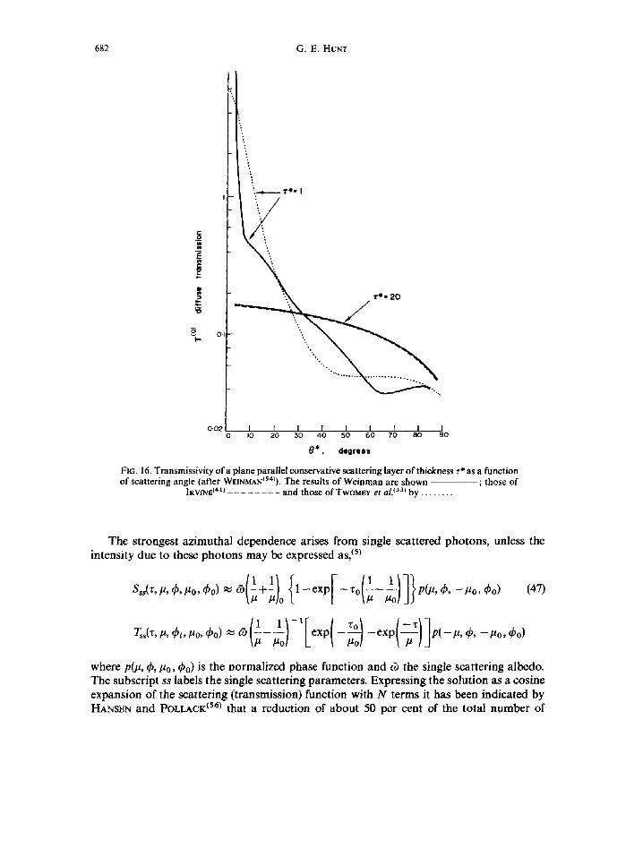
WErNr, tAN t54) developed an approach in which the forward peak was represented by a Gaussian distribution while the remainder of the phase function was expanded in a Legendre expansion. The division point between the two representations was arbitrarily chosen. Consequently, this may result in subsequent errors in computations of the angular distribution of the transmissed radiation for optical thickness of z < 10 and angular ranges in the neighbourhood of the division point where the distinction between large scale and small angle scattering is not clearcut, Fig. 16.

A more successful method is the 'truncated peak' technique developed by POTTER. t55} The approximate phase function is determined by truncating the forward peak, and then taking the gradient of the logarithm of the phase function to be constant for 0 < 0, where 0 is the truncation point. The fraction of photons scattered into the forward peak is

f df~ F = (p-p ' ) 4----n-' (44)

where p and p' are the untruncated and truncated phase functions respectively. In cloud optical thickness z is correspondingly reduced to ~' so that

r' = (1 - F)z. (45)

In the case of non-conservative scattering, the single scattering albedo must be scaled such that

[ ' - O 1 -~ ~ ' = 1 -~ o9(-i--~) (46)

since the assumption that photons in the forward peak should be treated as unscattered implies that the absorption cross-section is unchanged, while the scattering cross-section is reduced by a factor 1 - F.


60 X - 2-3/z / / / I ~ Mie phase function //

..... HG. phase function I/

4o

>~

~ 2o

- - L I i I ~ Tc I 0-1 I I0 IOO

Cloud optical thickness

FIG. 15. Comparisons of the emissivity of a terrestrial ice cloud at 2 = 2.3/t as a function of optical depth ~. The results are computed from a plane parallel scattering layer with Henyey-Greenstein

and Mie phase functions.

Numerical tests of this technique by HANSEN {5°) indicate that for conservative scattering the approximation introduces large errors for small total scattering angles 0 = 0 °. Errors of a few percent of the total scattering angle corresponds to a sharp feature in the phase function (and as the glory), or if the incident or emergent angle is near to grazing. In all other situations, the error is less than 1 per cent, see Figs. 12, 13, 14. For these calculations, the optical thickness was reduced by a factor 1 - F = 0.566.

We have already shown in Section 2, that the number of terms required to represent the phase function as a Fourier cosine expansion is N ,-~ 2 x + 12, where x is the size parameter. In the visible or near infrared regions of the spectrum where x ~ 100, the number of terms be N = 100-200. If we use a ' t runcated peak ' phase function then the number of terms in the cosine expansion may be 50 per cent less than that required to represent the atmospheric phase function POTTER. (55) The precise reduction N will depend upon the magnitude of the forward peak. However, both DAVE and GAZDAG (43) and HANSEN and POLLACK (s6) have independently shown that N is strongly dependent upon /~0, #, the cosines of the angle of incident and reflection. To illustrate this, we have shown in Fig. 17 the variation of N ~ , #') for 0 = cos- i # = 20, 40, 60, 80 with #' for a haze M in the visible. Employing this observation will reduce the amount of computer time; HANSEN and POLLACK (56) indicated that for their method a factor of 2-3 in C P U time was saved with an introduction of 1-2 per cent errors.

682 G.E. HUNT

[ 8

l

0 ~ " :':t •

0-02 I I I I I I I I I I0 20 30 40 50 60 70 80 90

0 " , degrees

FIG. 16. Transmissivity of a plane parallel conservative scattering layer of thickness z* as a function of scattering angle (after WEXNMANtS4J). The results of Weinman are shown ; those of

IRVINE (41) and those of TWOMEY et al. ~33) by . . . . . . . .

The strongest azimuthal dependence arises from single scattered photons, unless the intensity due to these photons may be expressed as, tS)

Sss(Z'lt'qb'lt°'qb°)'~69[l+ll, l~ It,o { 1 - e x p [ - z O ( 1 - 1 ) ] } p ( p , q ~ , - l ~ o , q ~ o ) (47,

T~s(T,~,q~,,/~o, 4~o)~(5 ~ - - ~ exp -- - e x p - ~ P(--/~,4~,--Po,4'o)

where p(p, 4',/1o, 4~o) is the normalized phase function and (5 the single scattering albedo. The subscript ss labels the single scattering parameters. Expressing the solution as a cosine expansion of the scattering (transmission) function with N terms it has been indicated by HANSEN and POLLACK (s6) that a reduction of about 50 per cent of the total number of


terms N required may be made by writing N'

s(~,~,4,,~o,~o) ~ s,~(~,~,d,,Uo,~o)+ Z [s~n~(~,~,~o,-S~(~,~,~o)]cosn(e~-ePo). (48) n=0

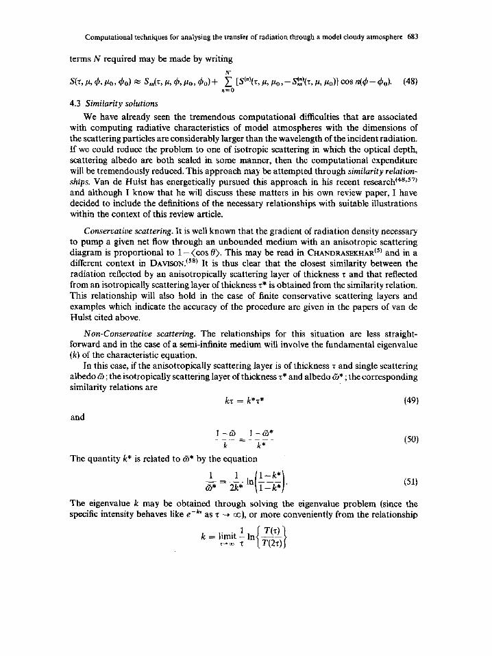
4.3 Similarity solutions

We have already seen the tremendous computational difficulties that are associated with computing radiative characteristics of model atmospheres with the dimensions of the scattering particles are considerably larger than the wavelength of the incident radiation. If we could reduce the problem to one of isotropic scattering in which the optical depth, scattering albedo are both scaled in some manner, then the computational expenditure will be tremendously reduced. This approach may be attempted through similarity relationships. Van de Hulst has energetically pursued this approach in his recent research (4s'57) and although I know that he will discuss these matters in his own review paper, I have decided to include the definitions of the necessary relationships with suitable illustrations within the context of this review article.

Conservative scattering. It is well known that the gradient of radiation density necessary to pump a given net flow through an unbounded medium with an anisotropic scattering diagram is proportional to 1 - (cos 0). This may be read in CaANDRAS~I~-IAR ~5~ and in a different context in DAVISON. (Sa) It is thus clear that the closest similarity between the radiation reflected by an anisotropically scattering layer of thickness z and that reflected from an isotropically scattering layer of thickness z* is obtained from the similarity relation. This relationship will also hold in the case of finite conservative scattering layers and examples which indicate the accuracy of the procedure are given in the papers of van de Hulst cited above.

Non-Conservative scattering. The relationships for this situation are less straightforward and in the case of a semi-infinite medium will involve the fundamental eigenvalue (k) of the characteristic equation.

In this case, if the anisotropically scattering layer is of thickness z and single scattering albedo &; the isotropically scattering layer of thickness z* and albedo (5*; the corresponding similarity relations are

kz = k'z* (49)

and

1 - - & 1 --&* - - = - - ( 5 0 )

k k*

The quantity k* is related to ~b* by the equation

1 = 1 1 [ 1 - k * l &---* 2k* n / 1 - - ~ )" (51)

The eigenvalue k may be obtained through solving the eigenvalue problem (since the specific intensity behaves like e -k" as z ~ m), or more conveniently from the relationship

k -- limit 1 . f T(z))

684 G . E . HUNT

I 0 0

8 0

6 0

4 0

2 0 ,

=

0 q

8 0 - -

8 0

~ 4 0 Z

Model: hoze M • • X -0 .7 '5 p..

• rn , 1.34 -O .O i oe

,* . ,

" 0 . 8 o . - . .

J j "

2O

4O

zo ' ~

e • zo ~

¢ I I I

0 20 4 0 60

. e-so* ." .

e e

".......,...- .,.

e . , o . /".. --....J

o.zo. ,. , . : ' ~

80 I00 f20 140 180 180 °

FIG. 17. The number of terms N(O', O) as a funct ion of 0', requi red to represent the phase funct ion corresponding to polydispersed water spheres model haze M, 2 = 0.75, m = 1.34 as a four ier

cosine expansion equation (27) with 0-1 per cent accuracy, (after Dave and GAZDAY(43)).

where T(z) is the integral over all emergent and incident angles of the CHANDRASEKHAR (5)

transmission function. For finite non conservative scattering layers we are only able to derive approximate

similarity relations We may write, VAN DE HULST (sT)

k 2 (1 - & ) ,,~ q- 0(k4). (52)

3(1 - (cos 0))

Then using this relationship and neglecting terms of 0(k 4) and eliminating k, k* from (50) and (50) yields the simple approximate similarity relation,

and z* = z(1 - ( c o s 0 ) )

1 - ~ 1 - ~ * =

1 - ( c o s 0)"

(53)

(54)


The advantage of these relationships is that they do not specifically require knowledge of k(o) and are therefore, much simpler to use. They are also extremely useful in line formation problems, when it is the intensity relative to the continuum intensity that is required. As such, this will not require knowledge of k(cb).

The accuracy of these similarity relations for conservative and non conservative scattering in semi-infinite atmospheres may be judged from the tables published in van de Hulst, CsT) which were produced from computations using the Henyey-Greenstein phase function. Further evidence of the similarity in the solution for various values ofg = (cos 0~ when y = (1 -&)/k is kept constant are illustrated in Fig. 18. These curves indicate the non- uniqueness of the interpretation of absorption lines in the reflected spectrum. (1 s>

Further tests on the accuracy of these relations has been made by HANSON (59) also from the context of absorption line formation. His results which were made for a homogeneous layer, indicate the increase in strength of the absorption line formed in the cloudy

IO 1" = (~0 I'0

~~0~5 tu"P'°(fixed) .0.5) ~ and g varying

08 08

0 • ~, ,875 06

I'C ~ ~ ~ 04

oB ~R(1,1) ~.

--'0~0 ' ~ - , o oz ,875 '5 0 6 ~ ~.,., 0

• I ~ " I i i # , ~ I L 0"4 0"6 0 '8

0'4

0"2 ~~'~=~5 0 0 2 0 4 0 6 0 8

y-( I -~) /k FIG. 18, Reduction of the reflectivity of an infinitely thick cloud layer as a consequence of absorption. The single scattering diagrams are computed with a Henyey--Greenstein phase function with

asymmetry parameter g. (after VAN DE HULST and GROSSMAN(4B)).

686 G.E. H t r ~ T

1.0

0.80 i 0.70 /

/

0

0.90 / / ""°" F , Y """' -

0 . 8 0 ,'

/ Oo.oo. [ j Oo.,,. 0 . 7 0 /

0 . 6 0 , I , , , a , , , , I , J . , . J ,

0 2 4 6 8 0 2 4 6 8 I 0 X

FZG. 19. Shape of weak absorption line (~o = @9975) for a thick atmosphere (~ = 640) with no continuous absorption (to, = 1-0) for normally incident radiation as a function of the direction of the incident radiation. Exact solution with no scaling ; solution from similarity equations (49), (50); . . . . . . . . . ; solution from similarity equations (53), (54) . . . . . . . . The results for the

cloud are displaced downward by 0-25 (after HANSEN(59)).

a tmosphe re as the degree of an i so t ropy of the scat tering particles increases. The exact equat ions (49), (50) and app rox ima te equat ions (53), (54) similari ty relat ions produce indist inguishable results for the compu ted line profiles, Fig. 19. The results are equally accurate for both s t rong and weak lines. C o m p u t a t i o n s of the light integrated over the p lanetary disk also indicate the accuracy of these relat ions for all except large phase angle

> 125 °, Fig. 20. At angles greater than this, 0t > 150 it is more accurate to employ isotropic scattering without any scaling of ~ , and T.

The results which are par t icular ly interesting involve the use of equat ions (53), (54) when appl ied to a finite scattering layer. The results shown in Fig. 21 indicate that the accuracy of the similarity relat ions decrease as • decreases. Fu r the r evidence of this is also shown in Fig. 22. Here we have compu ted the emissivity for ice cloud at 2.3/~ and compared it with the solut ion compu ted using (53), (54). A Deimendj ian cloud model was used with m a x i m u m radius 25/~ and mean extinction radius of 16 p. The error between


I0

050

025

o / I :

t " ,:.

I j , " " ~ e I . o , , l i I , t , t I , i , ~ , I , t , i I , /

~ l s o t r o p i c 0 7 5 /" / ~'Haze X / ~-Haze

- / / c,o.d ~/ ~.. ;= . / / / " ~ - - - ~ ~ . . . . . . . . •

050 ~ # 0 0 " /: $I --

0.2 ~ U - 150" _

I J I t I I I I t I t t I ~ t l I I t I I [ I I

0 I0 20 0 I 0 20 X

FIG. 20. Same as Fig. 18, but for the light integrated over the visible planetary disk at the phase angle ~t. The results of the cloud are displaced downward by 0-3 (after H A N S E N ( 5 9 ) ) .

the curves is greatest for small ~, as is also true of the reflectivity and transmissivity which are related to emissivity through the equation

e + r + t = 1. (56)

However, one may expect to produce considerably more accurate results using the "eigenvalue-similarity relations" as we have illustrated in the previous diagrams.

These illustrations of similarity relations have been made for homogeneous atmospheres. It remains to be demonstrated whether relations of this type may be efficiently used, and produce results of acceptable precision for scattering problems in inhomogeneous atmospheres.

CONCLUSION

We have outlined in this article the computational problems associated with analysing the radiative transfer in a model cloudy atmosphere.

The major developments have been associated with the construction of computational techniques. Methods of the type we have discussed in Section 3 have enabled research workers to tackle problems beyond the reach of analytical techniques and have encouraged

688 G . E . HUNT

J_w

Ic

1.0

~ t r o p i c / a ¢ " ' - - -Haze

o.2~ /.: 0 o- 3 0 * -

~.o , I ~ I J

~ o p i c 0.75 " / " ~ " Haze _

0 5 0

6 ' 0 - 75* 0 2 5 // -~

o _ -

0 :5 I0 I

0 15

~ i c

if . . . . .

// Oo.O.

J I ) I J

~ o p i c

, ) J I ,5 I0

FIG. 21. Same as Fig. 18 but for a finite a t m o s p h e r e zc = 10. The results of the c loud are d isp laced d o w n w a r d by 0.30 (after HANSEN(59)).

the use of more complex and accurate models. As we have seen two stages of approximation occur in these problems, in the formulation of the mathematical equations and in the process of numerical solution, and both stages need careful analysis if the results are to be of practical use. The first lies outside the province of the computing establishment, but the second can be very much influenced by the subroutine packages and hardware facilities provided.

In Section 3 we have outlined a number of possible techniques; but the choice made for a particular computational experiment should not be a matter of personal taste. Many factors are involved, the information required, the accuracy required, limits imposed by the numerical stability of the method, the speed of computation and computer storage available. Error estimates of the computational procedures are absolutely essential. Such estimates, if placed within an algorithm will inevitably lengthen the computation time, but since results of unknown accuracy are not really worth anything, the extra time is well spent. At the time of writing this article, only the procedures of GRANT and H U N T (3'28)

have been subjected to a detailed analysis of this type. The computational economies discussed in Section 4 indicate that considerable reduction

may be made in computational expenditure by simple approximations which introduce

Computat ional techniques for analysing the transfer of radiation through a model cloudy atmosphere 689

60 X = 2,3/z True solution iI//"'~"" S Similority solution / / "

ae 40

.~,

t) 2(3

/ /

/

i 1 , I , I 0 1 1 I0 I ~

Cloud optical t h i c k n e s s

FIG. 22. Emissivity of an ice cloud at 2 = 2.3 # as a function of optical thickness r. The similarity solution is computed using equations (55), (56).

errors of about 1 or 2 per cent. Such results are particularly useful to research workers who do not have access to large "number crunchers".

It would have been ideal to complete this review by assessing the accuracy of the model atmospheres by comparing the computed results with observation. We would then have a better idea of whether models are as realistic as we suppose. This is difficult to achieve since in many cases the essential details to enable such a comparison to be made have been rather vaguely described by the majority of experimental investigations. However, it is hoped that the future development of radiative transfer studies will enable a closer relationship between experimental and theoretical work than we have hitherto achieved. This we hope will lead to a greater understanding of the role of clouds and their interaction with both solar and planetary radiations fields and with motions which is central to the behaviour of an atmosphere.

Acknowledgements--We acknowledge the permission granted to us by Applied Optics to publish Figs. 2, 4, 5, 17 ; by J. Atmos. Sci. to publish Figs. 6, 12, 13, 14; J. Quant. Spectrosc. Radiat. Transfer to publish Figs. 8, 9, 10; Icarus to publish Fig. 16; Gordon and Breach Ltd. to publish Fig. 18 ; and A strophys. J. to publish Figs. 19, 20, 21.

R E F E R E N C E S

1. R. M. CrOODY, Atmosphere Radiation, p. 436. Oxford University Press (1964). 2. R. PREIS~NDORFER, Radiative Transfer in Discrete Spaces, p. 459. Pergamon Press (1965). 3. I. P. GRANT and G. E. HUNT, Proc. Roy. Soc. A313, 183 (1969).

690 G . E . HUNT

4. R. M. REDHEFFER, J. Math. Phys. 41, I (1962). 5. S. CHANDRASEKHAR, Radiative Transfer, p. 393. Dover, New York (1961). 6. LORD RAYLEXt3H (J, W. STI~UTT), Phil. Mag. 41, 107 (1871). 7. G. Mm, Annls. Phys. 25, 377 (1908). 8. H. C. VAN DE HULST, Light Scattering by SmallParticles. John Wiley (1957). 9. L. II~mLO, Quart. J. appl. Math. 5, 113 (1947).

10. D. DEIRMENDJIAN, Electromagnetic Scattering on Spherical Polydispersions, p. 290. Elsevier (1969). 11. G. W. KATTAWAR and G. N. PLASS, Appl. Opt. 6, 1377 (1967). 12. J. V. DAVE, Appl, Opt. 8~ 155 (1969). 13. J. V. DAVE, Appl. Opt. 8, 1161 (1969). 14. J. V. DAVE, Appl. Opt, 8, 2153 (1969). 15. W. M. IRVINE, Bull. Astron. Inst. Neth. 17, 176 (1963). 16. W. M. IRVINE, J. Opt. Soc. Am. 55, 16 (1965). 17. C. M. C , u and S. W. CrltmCrliLL, J. Opt. Soc. Am. 45, 58 (1955). 18. G. C, CLARK, C. M. Crru and S. W. CrrORCmLL, J. Opt. Soc. Am. 47, 81 (1957). 19. G. E. HUNT, JQSRT 10, 857 (1970). 20. V. V. SOBOLEV, A Treatise on Radiative Transfer. p. 319. van Nostrand (1963). 21. Z. SEKERA, RAND Pubis. R-413-PR. RAND Corp. Santa Monica, Calif. (1963). 22. J. W. CHAI~mERLAIN and M. B. McELRoY, Astrophys. J. 144, 1148 (1966). 23. A. L. FYMAT and K. D. AnrIYANKAR, Astrophys. J. 158, 315 (1969). 24. G. E. HtmT and I. P. GRANT, J. Atmos. Sci. 26, 963 (1969). 25. J. T. HOUGHTON and G. E. HUNT, Quart. J. R. Met. Soc. 97, 1 (1971). 26, G. E. HUNT, Beitr. Physik Atmosph. 42, 506 (1970). 27. V. A. A.~mARTSUr~aAN, Ddkl. Akad. Nauk. SSSR 38, 229 (1943). 28. I. P. GRANT and G. E. HUNT, Proc. Roy. Soc. A313, 199 (1968). 29. H. C. VAN DE HULST, A New Look at Multiple Scattering. NASA--Institute of Space Studies. New York

(1965). 30. G. C. STOKES, Proc. Roy. Soc. 11, 545 (1862). 31. H. C. VAN DE HULST, J. Comp. Phys. 3, 291 (1968). 32. J. E. HANSON, Astrophys. J. 155, 565 (1969). 33. S. TWOMEY, H. JACOBOWtTZ and H. B. HOWELL, d. Atmos. Sci. 23, 289 (1966). 34. I. P. GRANT and G. E. HUNT, Mon. Not. R, astr. Soc. 141, 27 (1968). 35. I. P. GRANT and G. E. HUNT, Icarus 9, 526 (1968). 36. I. P. GRANT and G. E. HUNT, JQSRTS, 1817 (1968). 37. R. E. BELLMAN, H. H. KAGIWADA and R. E. KALABA, Mort. Not. R. astr. Soc. 132, 183 (1966). 38. E. ISAACSON and H. B. KELLER, Analysis of Numerical Methods, p. 541, John Wiley, New York (1966). 39. B. RYmCKI and P. D. USHER, Astrophys. J. 146, 871 (1966). 40. D. G. HUMMER and G. B. RY~ICKI in Methods in Computational Physics, Vol. 7, 53-126. Academic Press,

New York (1966). 41. W. M. IRVINE, Astrophys. J. 152, 823 (1968). 42. B. M. HERMAN and S. R. BROWNING, J. Atmos. Sci. 22, 559 (1965). 43. J. V. DAVE and J. GAZDAG, Appl. Opt. 9, 1457 (1970). 44. G. N. PLASS and G. W. KATTAWAR, Appl. Opt. 7, 415 (1968). 45. D. G. COLLINS and M. B. WELLS, Monte Carlo Codes for the Study of Light Transport in the Atmosphere.

(Radiation Research Associates Inc. Vols. I, II.) 46. G. E, HUNT, JQSRTI I , 309 (1971). 47. L. G. HE~YEY and J. L. GREENS'traIN, Astrophys. J. 93, 70 (1941). 48. H.C. VAN DE HULST and K. GROSSMAN in The Atmospheres of Venus and Mars, pp. 35-36. Gordon & Breach,

New York (1968). 49. H. KAGIWADA and R. KALABA, RAND Report RM-5537-PR RAND Corporation. Santa Monica, California

(1967). 50. J. E. HANSEN, 3". Atmos. Sci. 26, 478 (1969). 51. L. M. ROMANOVA, Opt. Spek. 13, 429 (1962). 52. M. C. WANG and E. GUTH, Phys. Rev. 84, 1092 (1951). 53. W. M. IRVINE in The Atmospheres of Venus andMars, pp. 1057417. Gordon & Breach, New York (1968). 54. J. A. WFJMANN, lcarus. 9, 67 (1968). 55. J. POTTER, J. Atmos. Sci. 27, 943 (1970). 56. J. E. HANSON and J. B. POLLACK, J. Atmos. Sci. 27, 265 (1970). 57. H. C. VAN DE HULST, Bull. Astron. lnst. Neth. 20, 77 (1968). 58. B. DAVISON, Neutron Transport Theory. Oxford University Press. 450 (1957). 59. J, E. HANSON, Astrophys. J. 158, 337 (1969).

a review of computational techniques …dust.ess.uci.edu/ppr/ppr_hun71.pdfa review of computational...

Documents