a review of articulatory speech synthesis - aaltomath.aalto.fi/~jpalo/isod.pdf · a review of...
TRANSCRIPT

HELSINKI UNIVERSITY OF TECHNOLOGY
Department of Electrical and Communications Engineering
Laboratory of Acoustics and Audio Signal Processing
Pertti Palo
A Review of Articulatory Speech Synthesis
Master’s Thesis submitted in partial fulfillment of the requirements for the
degree of Master of Science in Technology.
Espoo, June 5, 2006
Supervisor: Professor Unto K. Laine
Instructor: Professor Martti Vainio, University of Helsinki

HELSINKI UNIVERSITY ABSTRACT OF THEOF TECHNOLOGY MASTER’S THESIS
Author: Pertti Palo
Name of the thesis: A Review of Articulatory Speech Synthesis
Date: June 5, 2006 Number of pages: 126
Department: Electrical and Communications Engineering
Professorship: S-89
Supervisor: Prof. Unto K. Laine
Instructor: Prof. Martti Vainio, University of Helsinki
Articulatory speech synthesis models the natural speech production
process. As a speech synthesis method it is not among the best, when
the quality of produced speech sounds is the main criterion. However,
for studying speech production it is the most suitable method.
This thesis reviews the literature on articulatory speech synthesis. The
objective is to look at articulatory speech synthesis form the viewpoint
of basic speech research. From this viewpoint, articulatory speech syn-
thesis is at its most interesting, when fidelity to natural speech produc-
tion process is considered a model’s most important aspect.
The thesis reviews methods for articulatory measurements, geometri-
cal synthesis of articulation and synthesis of speech sounds. The work
divides the measurement methods to static and dynamic methods ac-
cording to whether they are capable of capturing movement or not.
In surveying geometrical synthesis the text concentrates especially on
movement parametrisation and trajectory generation. Central topics in
speech sound synthesis are the transmission line method and a glimpse
at methods for non-linear sound generation.
Keywords: Articulatory speech synthesis, articulation, coarticulation,
articulators, articulatory modeling, articulatory measurements, audio-
visual speech, speech production, speech production model
TEKNILLINEN DIPLOMITYÖNKORKEAKOULU TIIVISTELMÄ
Tekijä: Pertti Palo
Työn nimi: Katsaus artikulatoriseen puhesynteesiin
Päivämäärä: 5.6.2006 Sivuja: 126
Osasto: Sähkö- ja tietoliikennetekniikka
Professuuri: S-89
Työn valvoja: Prof. Unto K. Laine
Työn ohjaaja: Prof. Martti Vainio, Helsingin Yliopisto
Artikulatorinen puhesynteesi mallintaa luonnollista puheentuottopro-
sessia. Puhesynteesimenetelmien joukossa se ei ole parhaasta päästä,
jos tuotetun puheäänen laatu on tärkein arvostelukriteeri. Sen sijaan
puheentuoton tutkimiseen se sopii synteesimenetelmistä parhaiten.
Tämä diplomityö luo katsauksen artikulatorisen puhesynteesin kirjal-
lisuuteen. Työn tarkoitus on tarkastella artikulatorista puhesynteesiä
puheen perustutkimuksen näkökulmasta. Tällöin artikulatorinen puhe-
synteesi on kiinnostavimmillaan, kun mallin uskollisuus luonnolliselle
puheentuottoprosessille on sen tärkein ominaisuus.
Teksti tarkastelee artikulaation mittaamisen, artikulaation geometrisen
synteesin ja artikulatorisen äänisynteesin menetelmiä. Mittaus-
menetelmät työ jakaa staattisiin ja dynaamisiin sen mukaan, pystyvätkö
menetelmät tallentamaan liikettä. Geometrisen synteesin osalta
tutkimus keskittyy erityisesti liikkeen parametrointiin ja liikeratojen
tuottamiseen. Keskeisiä aiheita äänisynteesissä ovat siirtolinjamalli ja
lyhyt katsaus epälinaariseen äänentuottoon.
Avainsanat: Artikulatorinen puhesynteesi, artikulaatio, koartikulaatio,
artikulaattorit, artikulaation mallintaminen, artikulaation mittaaminen,
audiovisuaalinen puhe, puheentuotto, puheentuottomalli

Acknowledgements iii
Acknowledgements
This Master’s thesis has been done for the Laboratory of Acoustics and
Audio Signal Processing of Helsinki University of Technology.
I want to thank my supervisor and instructor - professors Unto Laine and
Martti Vainio, respectively. With their guidance, support and patience they
have made this work possible.
I would also like to thank researcher Olov Engwall and professor Pierre
Badin. Professor Badin gave me the original spark of interest for articula-
tory speech synthesis during his visit to Finland some five years ago. Olov
fanned the flames with his presentation at the Mumin course in Tampere
some years ago and has since then provided a wealth of information on the
subject and very helpful comments on the text itself.
I wish to thank senior assistant Jarmo Malinen and assistant Teemu
Lukkari for their insightful conversation and help with reacquiring my
mathematics skills. A further, special thanks is due for the first gentleman
for the encouragement, which can be summarised as “Get it done.” Also,
on matters mathematical my thanks go to lecturer Seppo Uosukainen.
My gratitude also goes to the people who attended the cognitive science
master’s thesis seminar during the term of 2002–2003. I am especially grate-
ful to professor Christina Krause, who taught us all a lot about scientific
writing in general and of the ins and outs of a master’s thesis in particular.
Finally, I would like to thank my family and friends. Without the joy
and support you give me, staying sane would not be possible in a stressful
world.
Otaniemi, June 5, 2006 Pertti Palo

To Kaisa
for love and patience

CONTENTS v
Contents
Acknowledgements iii
Contents v
Symbols and Abbreviations ix
List of Figures xii
List of Tables xv
1 Introduction 1
1.1 Human Speech Production . . . . . . . . . . . . . . . . . . . . 1
1.2 Speech Synthesis . . . . . . . . . . . . . . . . . . . . . . . . . 4
1.2.1 Text-to-Speech Systems . . . . . . . . . . . . . . . . . 4
1.2.2 Speech Synthesis Methods . . . . . . . . . . . . . . . . 5
1.2.3 History of Speech Synthesis . . . . . . . . . . . . . . . 6
1.3 Articulatory Speech Synthesis . . . . . . . . . . . . . . . . . . 7
1.3.1 Definition . . . . . . . . . . . . . . . . . . . . . . . . . 7
1.3.2 Motives and Applications . . . . . . . . . . . . . . . . 8
1.4 Purpose and Structure of This Thesis . . . . . . . . . . . . . . 10
2 Data Acquisition Methods 12
2.1 Static methods . . . . . . . . . . . . . . . . . . . . . . . . . . . 12

CONTENTS vi
2.1.1 Direct Dimensional Measurements . . . . . . . . . . . 13
2.1.2 Computed Tomography (CT) . . . . . . . . . . . . . . 16
2.1.3 Ultrasound . . . . . . . . . . . . . . . . . . . . . . . . 19
2.1.4 Magnetic Resonance Imaging (MRI) . . . . . . . . . . 22
2.2 Dynamic Methods . . . . . . . . . . . . . . . . . . . . . . . . . 31
2.2.1 Cineradiography . . . . . . . . . . . . . . . . . . . . . 31
2.2.2 X-ray Microbeam . . . . . . . . . . . . . . . . . . . . . 35
2.2.3 Electromagnetic Articulography (EMA) . . . . . . . . 37
2.2.4 Electropalatography (EPG) . . . . . . . . . . . . . . . 41
2.2.5 Optopalatography (OPG) . . . . . . . . . . . . . . . . 44
2.2.6 Fast MRI . . . . . . . . . . . . . . . . . . . . . . . . . . 45
2.2.7 Motion Capture . . . . . . . . . . . . . . . . . . . . . . 49
2.2.8 Electromyography (EMG) . . . . . . . . . . . . . . . . 52
2.3 Aeroacoustic Measurements . . . . . . . . . . . . . . . . . . . 54
2.3.1 Airflow Measurements with Living Subjects . . . . . 54
2.3.2 Mechanical Models . . . . . . . . . . . . . . . . . . . . 56
2.4 Summary . . . . . . . . . . . . . . . . . . . . . . . . . . . . . . 58
3 Models of Vocal Tract Geometry 60
3.1 Modeling Vocal Tract’s Base Geometry . . . . . . . . . . . . . 60
3.1.1 Two Dimensional Models . . . . . . . . . . . . . . . . 61
3.1.2 Three Dimensional Models . . . . . . . . . . . . . . . 62
3.2 Parametrisation of Vocal Tract Movement . . . . . . . . . . . 65
3.2.1 Physiological Models . . . . . . . . . . . . . . . . . . . 66
3.2.2 Heuristically Defined Models . . . . . . . . . . . . . . 66
3.2.3 Statistically Defined Models . . . . . . . . . . . . . . . 71
3.3 Movement Generation . . . . . . . . . . . . . . . . . . . . . . 78
3.3.1 Heuristic Movement Models . . . . . . . . . . . . . . 79

CONTENTS vii
3.3.2 Physiological Models . . . . . . . . . . . . . . . . . . . 80
3.3.3 Concatenative Models . . . . . . . . . . . . . . . . . . 82
3.3.4 Coarticulatory Models . . . . . . . . . . . . . . . . . . 85
3.3.5 Gestural Models . . . . . . . . . . . . . . . . . . . . . 88
3.4 Handling Collisions . . . . . . . . . . . . . . . . . . . . . . . . 90
3.5 Summary . . . . . . . . . . . . . . . . . . . . . . . . . . . . . . 91
4 Acoustic Synthesis 93
4.1 Mathematical Basis of Modeling Vocal Tract
Acoustics . . . . . . . . . . . . . . . . . . . . . . . . . . . . . . 93
4.1.1 Basic Equations . . . . . . . . . . . . . . . . . . . . . . 94
4.1.2 Webster’s Horn Equation . . . . . . . . . . . . . . . . 95
4.1.3 Properties of Acoustic Tubes . . . . . . . . . . . . . . 95
4.1.4 Source Filter Model of Speech Production . . . . . . . 98
4.2 Linear Models . . . . . . . . . . . . . . . . . . . . . . . . . . . 98
4.2.1 Electrical Analog Circuits . . . . . . . . . . . . . . . . 99
4.2.2 Computer Simulation . . . . . . . . . . . . . . . . . . 100
4.3 Non-linear Models . . . . . . . . . . . . . . . . . . . . . . . . 103
4.3.1 Noise Generation Modeled with Vorticity . . . . . . . 103
4.4 Summary . . . . . . . . . . . . . . . . . . . . . . . . . . . . . . 105
5 Discussion 106
5.1 Data Acquisition . . . . . . . . . . . . . . . . . . . . . . . . . 106
5.2 Models of Vocal Tract Geometry . . . . . . . . . . . . . . . . . 107
5.3 Acoustic Synthesis . . . . . . . . . . . . . . . . . . . . . . . . 107
5.4 Further Topics of Interest . . . . . . . . . . . . . . . . . . . . . 108
5.4.1 Evaluating an Articulatory Speech Synthesiser . . . . 108
5.5 Possible Future Directions . . . . . . . . . . . . . . . . . . . . 109
5.5.1 Removing Idealisations . . . . . . . . . . . . . . . . . 109

CONTENTS viii
5.5.2 Physical Simulations . . . . . . . . . . . . . . . . . . . 109
5.6 Conclusion . . . . . . . . . . . . . . . . . . . . . . . . . . . . . 110
Bibliography and References 111
A Webster’s Horn Equation 123
A.1 Notes on Deriving the Equation . . . . . . . . . . . . . . . . . 126
Symbols and Abbreviations ix
Symbols and Abbreviations
A(x) Area function i.e. cross sectional area of the VT in relation to distance
from glottis
ρ density of the medium
ρ0 constant component of the density of the medium
p perturbation pressure (sound pressure)
q′ mass source
U volume velocity
u particle velocity
[A] Phone A
1D One Dimensional
2D Two Dimensional
3D Three Dimensional
4D Four Dimensional (usually three spatial dimensions and time)
5D Five Dimensional
A/D Analog to Digital converter
AFA Arbitrary Factor Analysis
C Consonant (e.g. CV sequence = consonant-vowel sequence)
CPU Central Processing Unit
CT Computer Tomography
Symbols and Abbreviations x
D/A Digital to Analog converter
DMM Dynamic Mechanical Model (of VT and glottis)
EBCT Electron Beam Computed Tomography
EMA Electromagnetic Articulography
EMG Electromyography
EPG Electropalatography
F0 Fundamental Frequency
F1, F2, F3, . . . Formant Frequencies
FEM Finite Element Model
fMRI functional Magnetic Resonance Imaging
FOV Field Of View
fps frames per second
HTML Hypertext Markup Language
ICA Independent Component Analysis
IPA International Phonetic Association
LCA Linear Component Analysis
LPC Linear Predictive Coding
MR Magnetic Resonance (as in MR image)
MRI Magnetic Resonance Imaging
NN Neural Network(s)
OPG Optopalatography
PARAFAC PARAllel FACtorial analysis
PCA Principal Component Analysis
SNR Signal to Noice Ratio

Symbols and Abbreviations xi
TSE Turbo Spin Echo (an MR imaging sequence)
TTS Text-to-Speech
V Vowel (e.g. VCV sequence = vowel-consonant-vowel sequence)
VF Vocal Folds
VT Vocal Tract
LIST OF FIGURES xii
List of Figures
1.1 The speech production organs . . . . . . . . . . . . . . . . . . 2
1.2 Typical articulation positions . . . . . . . . . . . . . . . . . . 2
1.3 Diagram of tongue muscles . . . . . . . . . . . . . . . . . . . 3
1.4 The vocal folds . . . . . . . . . . . . . . . . . . . . . . . . . . 4
1.5 Schematic of text-to-speech synthesis citeLemmetty:RSST:1999
5
1.6 Wheatstone’s reconstruction of von Kempelen’s speech syn-
thesizer (Flanagan, 1965) . . . . . . . . . . . . . . . . . . . . 7
1.7 Construction of an Articulatory Synthesiser . . . . . . . . . . 9
2.1 Pharynx seen through a fiberscope . . . . . . . . . . . . . . . 14
2.2 CT cross-section of the pharynx . . . . . . . . . . . . . . . . . 17
2.3 Cross-sectional contours of the pharynx obtained by CT . . . 18
2.4 Tongue surfaces reconstructed from 3D ultrasound data . . . 22
2.5 VT contours from experimental MRI . . . . . . . . . . . . . . 25
2.6 Semi-polar MR image grid . . . . . . . . . . . . . . . . . . . . 27
2.7 Equipment used to position a speaker for X-ray . . . . . . . . 33
2.8 Semipolar measurement grid for cineradiography . . . . . . 34
2.9 Maeda’s semipolar cineradiography grid and lip measure-
ment points . . . . . . . . . . . . . . . . . . . . . . . . . . . . 35
2.10 VT traced from an X-ray picture . . . . . . . . . . . . . . . . . 36

LIST OF FIGURES xiii
2.11 Dynamical semipolar mid-sagittal grid . . . . . . . . . . . . . 36
2.12 X-ray microbeam system diagram . . . . . . . . . . . . . . . 37
2.13 EMA principle . . . . . . . . . . . . . . . . . . . . . . . . . . . 38
2.14 5D EMA setup . . . . . . . . . . . . . . . . . . . . . . . . . . . 40
2.15 Example of an EPG palate . . . . . . . . . . . . . . . . . . . . 42
2.16 Concurrent EMA and EPG . . . . . . . . . . . . . . . . . . . . 43
2.17 OPG setup . . . . . . . . . . . . . . . . . . . . . . . . . . . . . 44
2.18 Pictures from real time MRI . . . . . . . . . . . . . . . . . . . 46
2.19 A picture from real time spiral echo MRI . . . . . . . . . . . . 47
2.20 Pictures from stroboscopic MRI . . . . . . . . . . . . . . . . . 48
2.21 Pictures from tagged MRI . . . . . . . . . . . . . . . . . . . . 49
2.22 Motion capture with lips painted blue . . . . . . . . . . . . . 51
2.23 Simultaneous EMA and motion capture . . . . . . . . . . . . 51
2.24 Examples of EMG data . . . . . . . . . . . . . . . . . . . . . . 52
2.25 Flow measurements in the mouth cavity . . . . . . . . . . . . 55
2.26 Dynamic Mechanical Model of the VT . . . . . . . . . . . . . 56
2.27 A flow measurement facility . . . . . . . . . . . . . . . . . . . 58
2.28 A resin reconstruction of the VT . . . . . . . . . . . . . . . . . 58
3.1 Engwall’s 3D vocal tract . . . . . . . . . . . . . . . . . . . . . 64
3.2 Badin’s 3D vocal tract . . . . . . . . . . . . . . . . . . . . . . . 65
3.3 2D vocal tract by Stevens . . . . . . . . . . . . . . . . . . . . . 67
3.4 2D vocal tract by Lindblom . . . . . . . . . . . . . . . . . . . 68
3.5 2D vocal tract by Mermelstein . . . . . . . . . . . . . . . . . . 70
3.6 2D vocal tract by Coker . . . . . . . . . . . . . . . . . . . . . . 70
3.7 2D vocal tract by Rubin . . . . . . . . . . . . . . . . . . . . . . 71
3.8 Parameters for HLsyn . . . . . . . . . . . . . . . . . . . . . . 72
3.9 Tongue parameters from PARAFAC . . . . . . . . . . . . . . 73

LIST OF FIGURES xiv
3.10 Tongue parameters from AFA . . . . . . . . . . . . . . . . . . 75
3.11 PCA tongue parameters by Kaburagi . . . . . . . . . . . . . . 76
3.12 3D VT parameters by Badin . . . . . . . . . . . . . . . . . . . 76
3.13 3D tongue parameters by Engwall . . . . . . . . . . . . . . . 77
3.14 3D tongue parameters by Badin . . . . . . . . . . . . . . . . . 78
3.15 Tongue model based on opposing muscle pairs . . . . . . . . 81
3.16 Generation of articulatory trajectories for the tongue . . . . . 82
3.17 Tongue model based on muscle modeling . . . . . . . . . . . 83
3.18 Effect of exponential dominance functions . . . . . . . . . . . 87
3.19 Spline-like dominance functions . . . . . . . . . . . . . . . . 87
3.20 Movement constraints of Kaburagi’s model . . . . . . . . . . 88
3.21 Parameters of Kaburagi’s model . . . . . . . . . . . . . . . . 89
3.22 Voxel space used in collision detection . . . . . . . . . . . . . 91
3.23 Palate grid tuned for collision detection . . . . . . . . . . . . 92
4.1 Tube model of the VT and a reflecting tube junction . . . . . 96
4.2 Schematic of the source-filter model of speech production
Lemmetty (1999) . . . . . . . . . . . . . . . . . . . . . . . . . 98
4.3 Acoustic tube’s electrical model by Dunn . . . . . . . . . . . 99
4.4 Electrical model of the VT by Dunn . . . . . . . . . . . . . . . 100
4.5 Acoustic tube’s electrical model by Stevens et al. . . . . . . . 100
4.6 The Kelly-Lochbaum junction . . . . . . . . . . . . . . . . . . 101
4.7 The VT simulation circuit proposed by Badin & Fant . . . . . 102
4.8 Simulated formants from 1D and 2D waveguide models . . 103
4.9 Vorpal sound generation . . . . . . . . . . . . . . . . . . . . . 104
4.10 Sinder’s aerodynamic sound generation model . . . . . . . . 105

LIST OF TABLES xv
List of Tables
3.1 Values of α and β used by Lindblom and Sundberg (1971) . 62
3.2 Definitions of A(d) used by Mermelstein (1973) . . . . . . . 63
3.3 Articulatory parameters of CASY (Rubin, Saltzman, Gold-
stein, McGowan, Tiede, & Browman, 1996). . . . . . . . . . . 71
3.4 Articulatory parameters of HLsyn (Stevens & Hanson, 2003). 72
4.1 Correspondence of Acoustical and Electrical Parameters af-
ter Deller, Hansen, and Proakis (2000) . . . . . . . . . . . . . 97
A.1 Definitions for analysis of wave propagation in the VT . . . 123
1 Introduction 1
Chapter 1
Introduction
To understand articulatory speech synthesis we have to understand human
speech production. This is obvious, if you consider that we are trying to
imitate speech production and it is very hard to imitate anything without
understanding the object of imitation.
It is also good to know a little bit about speech synthesis in general. After
all, articulatory speech synthesis shares many of its methods with other
forms of speech synthesis. For these reasons I have written the following
two sections as an introduction to someone who has limited experience of
either subject.
1.1 Human Speech Production
Figure 1.1 shows the human speech production organs along with an ideal-
ized model. The picture on the left shows the main articulators - the tongue,
the jaw and the lips - as well as other important parts of the vocal tract (VT).
The picture on the right shows the model, which is the basis of almost every
acoustical model of the vocal tract.
In production of pulmonic sounds breathing muscles act as an energy
source while the lungs provide a storage of pressurised air1. The lungs are
separated from the vocal tract by the vocal folds, which are also known as
1In production of non-pulmonic sounds such as clicks the energy source is provided by
the tongue muscles as they press an air pocket against other VT structures and then release
the pressure producing the click sound.

1 Introduction 2
Figure 1.1: The human speech production organs and an idealized model
(Rossing et al., 2002, p. 337)
vocal chords. The vocal folds generate a signal, which is then filtered by the
vocal tract and finally radiated to the surroundings via the mouth and/or
nostrils.
While the above description of the speech production process is fairly
accurate for (some stages of) vowel production, it is only a starting point
to understanding speech production in general. The neurological process,
which leads to articulation movements, is not a part of the described pro-
cess. It is also outside the scope of this work - and most others - but hope-
fully in the future a part of a “complete model of speech production”.
Figure 1.2: Typical articulation positions (O’Shaughnessy, 1987). (a) and
(b) illustrate different kinds of vowels, (c) shows possible stop consonant
articulations and (d) an alveolar fricative.
However, there are several things that can be added the above descrip-
tion that do fall in the scope of this review. For instance, the possible artic-
ulation positions and the physiology of the articulators themselves need to

1 Introduction 3
Figure 1.3: Diagram of tongue muscles and some related structures
(O’Shaughnessy, 1987). The muscles and structures are: 1: inferior lon-
gitudinal muscle, 2: dorsum, 3: styloglossus muscle, 4: styloid process of
temporal bone, 5: hyoglossus muscle, 6: stylohyoid muscle, 7: stylopha-
ryngeal muscle, 8: thyroid cartilage, 9: hyoid bone, 10: geniohyoid muscle
and 11: genioglossus muscle.
be considered. Figure 1.2 illustrates some typical articulation positions and
figure 1.3 gives a glimpse at the complexity of the involved physiology.
Furthermore, as mentioned above, the description is for vowels only. Ac-
cording to Olive et al. (1993) consonants cause all sorts of havoc in such a
simple model. Firstly plosives (e.g. [p, t, k]) are based on closing the VT
at some point above the vocal folds. Secondly fricatives (e.g. [f, s]) add a
turbulent noise source to the system at their point of articulation. Thirdly
nasals (e.g. [n, m]) keep the mouth closed while the sound radiates through
the nostrils. Fourthly sounds, which are called liquids in American En-
glish (e.g. [l, r]), divide the mouth cavity into two tubes instead of one.
One could continue the list with the [r] of Finnish and many other sounds,
which are more or - usually - less like vowels.
Then one needs to also note that not all sounds are voiced i.e. the vocal
folds vibrate only during the production of vowels and voiced consonants.
Indeed there are several different modes of operation for the vocal folds.
Figure 1.4 illustrates the difference between three of these.

1 Introduction 4
Figure 1.4: The vocal folds. The three shown operation modes are a) breath-
ing (folds stay open) b) normal speech phonation and c) whisper phona-
tion. (from Kahle et al. (1984) in Mixdorff (2002))
Finally, there is still one thing of utmost importance which makes the
above description fall somewhat short: Articulation is not a static thing
and speech sounds are not produced by isolated incidents of ideal articula-
tion. Rather the articulation of a phone is a function of time and a process
known as coarticulation. That is the effect that surrounding phones have
on the currently articulated one. For example, [t] in the utterance [ata] is
articulated differently from the [t] in the sequence [utu].
1.2 Speech Synthesis
A speech synthesis system is by definition a system, which produces syn-
thetic speech. It is implicitly clear, that this involves some sort of input.
What is not clear is the type of this input. If the input is plain text, which
does not contain additional phonetic and/or phonological information
the system may be called a text-to-speech (TTS) system. However, in the
strictest sense the term “speech synthesis system” applies only to the part
of a TTS system, which produces the speech signal from some sort of a
phonetic description. While this strict definition will be used in this thesis,
it is useful to take a look at TTS as it is the most common context for speech
synthesis.
1.2.1 Text-to-Speech Systems
A schematic of the text-to-speech process is shown in figure 1.5.
As seen in the picture the synthesis starts from text input. Nowadays
this may be plain text or marked-up text e.g. HTML or something similar.
If the text uses some sort of mark-up it may already contain some or all

1 Introduction 5
Figure 1.5: Schematic of text-to-speech synthesis citeLemmetty:RSST:1999
of the information made available by the text and linguistic analysis stage.
Regardless of the quality of the input text, after this stage we will have
a description of the text on the phonetic level. A fairly popular way of
representation is again a mark-up of some sort.
The second stage is prosody and third stage speech signal generation.
During the prosody stage linguistic information is used to generate F0
contours, timing information for the phones etc. Finally, the synthesized
speech itself is generated from these specifications. If we are dealing with
normal TTS, the generated speech will take the form of a audio signal,
but on the other hand, if we are dealing with text-to-audio-visual-speech
then the generated audio will be accompanied by a synchronized video
sequence.
1.2.2 Speech Synthesis Methods
The above description holds for most TTS systems. The most important
differences are usually in the way that the audio (and video) signal is gen-
erated. In a way the easiest method to understand is concatenative SS. In
essence it is cut-and-paste synthesis. The audio (or video) signal is formed
by concatenating prerecorded speech samples. The hard parts are in se-
lecting a good database and selecting the best samples from the database.
Usually the database consists of phonemic units or diphones i.e. transitions
from one phone to another, but it may also contain longer section such as
complete words or shorter ones.
Another method, which is more closely related to articulatory speech
synthesis, is formant synthesis. Its goal is to produce an speech by gen-
erating with rules a signal, which mimics the formant structure and other
spectral properties of natural speech as closely as possible.
1 Introduction 6
1.2.3 History of Speech Synthesis
There are several good texts on the history of speech synthesis - Klatt (1987)
and applicable parts of Flanagan (1965) to mention just two. Thus here we
will only take a brief look at some interesting landmarks.
The history of speech synthesis machines begins at least as early as the
17th century (Fagyal, 2001). Unfortunately, these early attempts did not
leave anything but indirect documentary evidence of their existence. If
they even ever did exist as anything but plans, they were considered some
kind of musical instruments by their designers and users. Nevertheless, the
early machines were an omen of things to come. Until the late 19th century
SS was based on construction of physical models, which can be considered
simple articulatory speech synthesizers.
The beginning of text-to-speech systems can be placed in late 18th cen-
tury. In 1779, the Academy of Sciences of St Petersburg held a contest for
building and demonstrating a speaking machine capable of producing five
vowels on its own. The prize went to the well known tube machine of C.
G. Kratzenstein. Kratzenstein’s machine produced only static vowels, but
another contestant - Wolfgang von Kempelen - demonstrated a machine
capable of producing dynamic speech. Figure 1.6 shows Wheatstone’s re-
construction of von Kempelen’s machine2.
The late 19th century gave birth to all sorts of electrical devices and
among them was a electromechanical speech synthesiser by Helmholtz.
Another one of the first electrical analogs of the human speech organs
was presented by Stewart (1922), who appears not to have known of
Helmholtz’s earlier vowel synthesis machine. Stewart’s device consisted
of an interrupted source and two adjustable RCL-resonator circuits. These
can be seen to correspond to the vocal folds (the source and interrupter)
and the VT (the resonators).
The next great landmark in the history of speech synthesis systems is the
boom in 1950’s. But this brings us already to the scope of this thesis. Two
of the systems from this era are described in section 4.2, page 98.
2This reconstruction had an interesting role in the history of speech technology (Deller
et al., 2000). Alexander Graham Bell had the chance of seeing Wheatstone’s reconstruction
as a boy in Edinburgh, Scotland. This event set him on the track, which lead to the U.S.
Patent 174465 (the voice telephone).

1 Introduction 7
Figure 1.6: Wheatstone’s reconstruction of von Kempelen’s speech synthe-
sizer (Flanagan, 1965)
1.3 Articulatory Speech Synthesis
1.3.1 Definition
While this is a master’s thesis in engineering rather than in philosophy I
still find it useful to give my definition of the topic. Although I have tried
to make this definition as precise as possible I still might include material
that does not strictly fall under it.
The definition of articulatory synthesis that I decided to adopt for this
work is as follows:
“Articulatory speech synthesis models the natural speech production
process as accurately as possible. This is accomplished by creating a syn-
thetic model of human physiology and making it speak.”
This definition gives a set of goals for articulatory speech synthesis:
1. Accuracy of the model in comparison with the speaker(s) on, which
it is based.
2. Naturality of the model.
3. Intelligibility of the model.
4. New information and understanding gained from the model.

1 Introduction 8
1.3.2 Motives and Applications
Articulatory speech synthesis may be utilised in a project aiming at a fin-
ished application e.g. a commercial speech synthesiser. Thus, motives and
applications for a speech synthesiser are in principle valid motives and ap-
plications for research into articulatory speech synthesis. Nevertheless, it
is worth noticing, that if the motivation for a project is for example better
quality of synthesised speech within a time frame of few years, articulatory
speech synthesis probably is not the answer. Nowadays there are methods
like LPC and concatenative synthesis, which are more successful with the
quality of output than articulatory speech synthesis. This work, however,
concentrates on articulatory synthesis in the context of basic research. And
this is the area of application and the motivation where articulatory speech
synthesis is very good.
Articulatory speech synthesis may be used as a tool in basic speech re-
search and is in itself a subject of basic speech synthesis research. Articu-
latory modeling is a good way to gain insights in to the speech production
and perception processes. If we are able to understand speech production
at the deepest levels, we will be able to construct an articulatory speech
synthesiser, which is indistinguishable from a natural speaker. The reverse
can be stated with equal certainty: A good enough articulatory speech syn-
thesiser will enable us to understand the speech production process in its
smallest details.
On the other hand, it is important to know which properties of the artic-
ulatory process have to be modeled in order to achieve high quality speech
synthesis. Detailed articulatory speech synthesis would make answering
this problem, if not easy, at least fairly straight forward. Of course there
would still be a considerable amount of work involved. The necessary per-
ceptual studies would, in contrast, be much simpler with the degree of con-
trol that a synthesiser would make possible when compared with a natural
speaker.
When considering the naturalness of a synthesiser one important ques-
tion to consider is whether geometrical modeling is necessary. The fact is
that there are some - especially prosodic - features of speech, which are
nearly impossible to reproduce with articulatory synthesis without geo-
metrical modeling. Some of them are very hard to extract from the acoustic

1 Introduction 9
signal, but still clearly perceptible to a human listener. Moreover, it can be
argued that it is simpler to remove features, that are found to be unneces-
sary, than it is to add - possibly unknown and unrecognised - features to a
model.
Another important aspect to consider is, that articulatory models are not
used only for speech production. They are also used for speech recognition
(see e.g. (Blackburn, 1996)) as a part of the effort of trying to understand
the twin process of speech production and recognition by modeling it as
a whole. In this particular context articulatory speech synthesis may be
seen as a model for the information encoding in the acoustic speech signal.
Figure 1.7 shows a rough sketch of the parts of such a model along with
some of the types of data needed for the construction of each part of the
model.
Data Acquisition ⇒ Data Analysis ⇒ Synthesis Stages
Static
Geometry⇒
Target
Values
⇒Synthesis of
GeometryDynamic
Geometry⇒
Movement
Generation
Mechanical
Models
Fluid Flow
Dynamics
Sound
Recording
⇒Sound Source
Model
⇒Sound
Synthesis
︸ ︷︷ ︸
Model of Information Encoding in the Speech Signal
Figure 1.7: A schematic of the construction of an articulatory speech syn-
thesiser and how a such a synthesiser may be considered to contain a model
of information encoding in the speech signal.
If we take a wider view of speech research, then two additional reasons
for including geometrical synthesis in the model are present. An articu-
latory speech model could also be used to study speech pathology in the
same way as perception models can be used to study perception pathology
(see e.g. Eysenck and Keane (2000)). This would obviously benefit from
the possibility to view the problematic areas. Moreover, if the geometrical
model is a part of the synthesiser, it is simple to generate also video output
and enable the model to be used in multimodal research.

1 Introduction 10
Besides the more immediate gains in basic research, it is good to also
keep in mind some of the possible uses of an articulatory speech synthesiser
as a finished product. These include use as a virtual language tutor (Eng-
wall, Wik, Beskow, & Granström, 2004), in speech therapy, in general pur-
pose audio-visual speech synthesis, in speech encoding (Schroeter, Larar, &
Sondhi, 1987), (Schroeter, Larar, & Sondhi, 1988), (Parthasarathy, Schroeter,
Coker, & Sondhi, 1989), in imitation of real speakers, as the speech engine
of virtual actors and even as a toy.
To summarize, the most important contribution of articulatory models is
the same as that of any model in general. They are ways of unifying knowl-
edge and as such act as test beds of theories. Without modeling and com-
paring the results of the model with the original it is hard to say whether a
theory is useful or not.
1.4 Purpose and Structure of This Thesis
As the title of this thesis suggests, I will not review the use of articulatory
modeling in speech or speaker recognition. Neither will I spend very much
time describing synthesis methods, which do not aim at modeling speech
with methods based on modeling articulation. A final area of research,
which I excluded from the scope of this work, is modeling the vocal folds
and/or the glottal signal source. This exclusion was done purely to limit
the amount of work, that was necessary in finishing this work. However,
none of these exclusions are absolute. Therefore, I will discuss any - and
hopefully most of the interesting - research that sheds light on the topic of
this thesis.
The disposition of the following chapters follows roughly the modular-
isation described by figure 1.7. The applicable parts of the figure’s first
column are the topic of chapter 2, page 12, where I will describe several
ways that are or have been used in different projects to obtain information
for articulatory synthesis. The focus of this chapter will be the quality of
data obtained by a given method and the ethical, technical or other kinds
of problems arising from the use of the method.
1 Introduction 11
In chapter 3, page 60 I will describe methods, which have been employed
in constructing the geometrical part of articulatory synthesis systems. Dif-
ferent types of static geometries will be reviewed as well as movement
parametrisations and movement generation methods. Finally a short look
will be taken at handling collisions between articulators.
In chapter 4, page 93 I will review acoustic synthesis methods. The chap-
ter will start with a look at the mathematics of vocal tract acoustics. After
that sound synthesis methods will be reviewed. The main focus will be on
methods, which have lead into more accurate descriptions of the speech
production process. Thus, methods, which have focused on other issues,
such as real time synthesis, will be left out.
Chapter 5, page 106 is the concluding chapter. There I will discuss the
theories covered as well as some of the ones left out of this thesis. I will
also present some directions of future research, which seem to be emerging
form the field.

2 Data Acquisition Methods 12
Chapter 2
Data Acquisition Methods
The first step in constructing a model is acquiring data on the phenomenon,
which is about to be modeled. Accordingly, data acquisition should play an
important role also in the construction of an articulatory speech synthesiser.
Important considerations in choosing the data acquisition method for
such a project are the application area of a method (which part or parts
of the articulatory system it can be used to explore), temporal and spatial
accuracy, safety issues, and other issues affecting the usage of the method.
In addition, the properties and nature of the raw data obtained in actual
studies should be considered. If these considerations are done carefully the
next steps of the construction process - building the geometric and acoustic
synthesis models - will be made considerably easier.
2.1 Static methods
These are methods, which capture static snapshots of articulation. The
defining characteristic and main problem of these methods is, that they are
unable to represent movement. Instead only isolated samples of articula-
tion may be obtained. Moreover, a fairly common problem is a requirement
of prolonged articulation, which may lead to unnatural results. This may
be caused by the subject getting tired, but also by their anticipation of pro-
longing articulation and other, method related, factors.
To minimise the unnaturalness caused by movement between repetitions
and during measurement, subject fatigue, and subject’s position various

2 Data Acquisition Methods 13
measures can be taken. Very often the articulations can be verified in-
directly by comparing the sound produced during data acquisition with
sound produced under more natural conditions. During data processing
movement artifacts can be removed by fixing the coordinate system to
bones instead of subject’s position within the measurement device. With
some of the methods it is also possible to shorten the acquisition time by
sacrificing resolution and thus reduce all of the effects caused by a long
acquisition time.
Even though the static methods have some intrinsic problems, they are
very important tools. This is due to the fact, that there are currently no real
4D methods. That is, there are no methods, which would gather spatially
three dimensional data in real time. Because of this, static methods have to
be used to obtain 3D snapshots of articulatory positions. These snapshots
can then be used - for example - as the target positions in a coarticulatory
model or in a similar manner.
2.1.1 Direct Dimensional Measurements
Direct dimensional measurements have been employed in a wide variety of
studies to record articulatory data. However, the success of these methods
has not always been as great as their ingenuity of design. The single most
prominent problem is their interference with the articulation itself. On the
other hand they have the advantage of being usually easy to calibrate.
Gauffin and Sundberg (1978) used a fiberscope to obtain pictures of the
pharynx. Gauffin and Sundberg (1978) inserted the fiberscope tube through
the subject’s nose and velar opening. They subsequently took pictures at
two levels in the pharynx during sustained phonation of isolated vowels.
In order to obtain panoramic views of the pharynx and the vocal cords
they swung the fiberscope tip from left to right and afterwards combined
the obtained partial views. Two example pictures obtained by Gauffin and
Sundberg (1978) can be seen if figure 2.1. An important finding by Gauffin
and Sundberg (1978) was that the relative dimensions of the VT differ at
higher and lower levels in the pharynx.
While the fiberscope method is quite safe and only causes some discom-
fort, it is not a very universal method. The methods area of application is
restricted to the structures visible beneath the velar opening. Furthermore,

2 Data Acquisition Methods 14
Figure 2.1: Two examples of the pictures along with diagrams of the visi-
ble anatomy and the points where the pictures were obtained (Gauffin &
Sundberg, 1978).
it would probably be difficult to use the fiberscope method to observe con-
sonant articulation as the articulators would be disturbed by the fiberscope
tip and thus the articulation would not remain natural.
As for the nature of the data obtained by the fiberscope method, it is only
qualitative, if a scale of reference is not obtained by some other method
(Gauffin & Sundberg, 1978). Gauffin and Sundberg (1978) used X-ray trac-
ings to obtain a scale of reference and suggested that the X-rays should be
taken simultaneously with the use of the fiberscope to further determine
the position of the fiberscope tip.
Casts of the Vocal Tract
Casts of the VT have been widely employed in speech production research.
It has been used to acquire data on the shape of the oral cavity and con-
striction caused by the teeth. With recent versions of the method, which
combine MRI with the more mundane process of taking a dental cast, the
method has become something of a standard tool. The taking of the cast
itself is a standard procedure of dental medicine and has not usually been
varied when using the technique for speech research1.
Stark, Ericsdotter, Branderud, Sundberg, Lundberg, and Lander (1999)
made dental casts of anterior VTs in order to be able to form good conver-
sion rules from cross-dimensions to cross-section areas, ie. d(x) to A(x).
1There have, however, been a couple of studies where the technique was employed to
produce a cast of the whole oral VT and hence had to be used differently from the standard
medical procedure (Ladefoged, Anthony, & Riley, 1971)

2 Data Acquisition Methods 15
They combined the information gained from the dental casts with their
main data source of cineradiography to produce estimated sagittal cross-
dimension to area functions for the whole VT.
Sundberg, Johansson, Wilbrand, and Ytterbergh (1987) used plaster casts
of the subjects palates in a similar way to the use of dental casts by Stark
et al. (1999). Instead of making a cast of the whole mouth Sundberg et al.
(1987) made a plaster cast only of the palate. Afterwards the cast was filled
with plastic. The plastic was then cut up into radial slices. The slices were
determined by a circle which was tangent to the horizontal part of the hard
palate and the vertical part of the posterior pharynx wall. These slices were
used to determine the cross section area of the VT.
To test the effect of the slicing procedure on the results Stark et al. (1999)
also made plastic slices with the the angle of cutting being orthogonal to
the plane of the teeth. This, however, did not effect the results significantly.
What may be of greater importance, was that Stark et al. (1999) did not
have a way of directly relating the amount of plastic to the position of the
tongue. Rather they had to do it in a heuristic way using experience and
knowledge of the tongue’s position in the pharynx gained from their other
data source, computed tomography.
Parallel to the use of casts to augment data from cineradiography (Stark
et al., 1999) and regular tomography (Stark et al., 1999), they have been
employed to augment MRI data. As MRI inherently lacks data on teeth the
dental casts are vitally needed.
Baer, Gore, Gracco, and Nye (1991) took dental casts of their subjects.
Dental impressions made by using the casts as molds were sliced and the
slices digitised by manually tracing them with a graphics tablet. The result-
ing images were then used to correct corresponding slices obtained with
MRI.
In a similar approach Narayanan, Alwan, and Haker (1995) made dental
casts of their subjects and measured some relevant distances straight from
the casts. In addition they also made dental impressions. The impressions
were subsequently sliced and used paper tracings of coronal and sagittal
slices to correct MRI results.
The latest innovation is using MRI to measure the casts and hence easing
the task of fitting the teeth with the MR images. Engwall and Badin (1999)
2 Data Acquisition Methods 16
gives a very detailed description of the required procedures. In short, the
casts are immersed in a water tank, which is then imaged with the same
scanner, which is used for imaging the VT. Afterwards, the resulting im-
ages are fitted together to form images of the VT with the teeth in place.
The same procedure has also been used by Badin, Bailly, Raybaudi, and
Segebarth (2002).
2.1.2 Computed Tomography (CT)
Computed tomography is a 3D imaging method which is based on X-ray
imaging. An intermediate step in the historical development of computed
tomography was ordinary tomography. It was a method of producing to-
mograms - pictures of a slice through the imaged object - on regular X-ray
film. X-ray imaging and ordinary tomography have been used in articula-
tory studies and are discussed in section 2.2.1, page 31.
Like ordinary tomography, CT produces 2D slices of the subject. The
slices are the result of computing the tissue density by solving the inversion
problem for X-ray absorption data. The absorption data is gathered by
rotating an X-ray source around the subject and registering the amount of
radiation passing through the subject on sensors positioned opposite to the
X-ray source. 3D images are produced by obtaining several parallel slices
of the same subject.
While early instruments were naturally slower more modern ones have
a fairly fast slice acquisition time. Even so, they have been far from being
instantaneous in acquiring a 3D image. This is changing with the introduc-
tion of multislice-CT, which can at present acquire up to 16 slices in one
pass.
CT produces images with a good contrast between air and bodily tissues
in general. For the purposes of imaging the VT this is especially good as
the walls of the VT will be clearly defined and easy to extract.
Moreover, CT has good resolution. Modern equipment are capable of
producing a slice thickness of 1mm and plane pixel size of 0.2mm. These
are, however, parameters for clinical use of CT. If used for non-medical
purposes - such as speech production studies, it may be necessary to be
more strict about the radiation doses and thus accept lower resolutions.

2 Data Acquisition Methods 17
CT’s main flaw is its use of X-rays. There will inevitably be an amount
of ionising radiation absorbed by the subject. The obvious need to keep the
radiation dose for the subject in acceptable limits restricts the number of
images that can be acquired from one subject.
Studies
Sundberg et al. (1987) took computed tomograms of two subjects (a male
and a female) in an effort to establish the area function A(x) relating the
VT’s sagittal cross-dimension to its cross-sectional area. The study was
limited to tomograms at four layers of the pharynx during the sustained
production of four vowels. The tomogram layers were 2mm thick and re-
quired a complete set of four required an acquisition time of 3.2 seconds.
During the whole study the maximum absorbed dose of radiation for the
subjects was 70 mGy.
As can bee seen in figure 2.2 the images were of good quality with a clear
VT contour. Figure 2.3 shows the VT contours for the male subject.
Figure 2.2: A CT cross section of a male pharynx 5.7 cm above the glottis
while pronouncing [i:] (Sundberg et al., 1987). Air is represented by white
and bone and tissues by other shades.
Interesting results from Sundberg et al. (1987) include the following: The
VT’s sagittal cross distance cannot be mapped to the lateral width by means
of simple linear regression and, furthermore, the mapping varies between
subjects. In contrast, such a mapping will produce good results, if it con-
cerns only one subject and a specific level in the pharynx.

2 Data Acquisition Methods 18
Figure 2.3: Cross-sectional contours of a male pharynx obtained by CT
Sundberg et al. (1987). The cross-sections were all taken in the axial plane
with levels ranging from the glottal region (level 1) to upper pharynx (level
4). All imaging levels were separated by 1.9 cm.
A more recent study by Tom, Titze, Hoffman, and Story (2001) (see also
(Tom, Titze, Hoffman, & Story, 1999)) had as its objectives the acquisition of
high resolution 3D images of the VT during phonation at variable pitch,
loudness and register (chest or falsetto) conditions. After consideration
they decided to use Electron Beam Computed Tomography (EBCT). The
main reasons were EBCT’s fast image acquisition time and good contrast
between bodily tissues and air when compared with the then current MRI
devices.
With the device used by Tom et al. (2001) the slice acquisition time was
100 ms, which, along with the slice thickness of 3 mm, made it possible
to image the whole VT in 12 to 18 seconds. The 3D image thus acquired
consisted of 60 slices with a resolution of 512x512 pixels each and a pixel
size of 0.410 mm. Known error from a test with a phantom VT was 1.8-2.0
%.
Further processing of the acquired image set was performed with an im-
age display and measurement tool called VIDATM. The VT region was
identified in the images by a seeded region growing method. The 3D shape
of the VT was then reconstructed with shape-based interpolation with the
resulting image set having the same 0.410 mm resolution in all directions.
The cross-sectional areas A(x) were measured from the final set.

2 Data Acquisition Methods 19
2.1.3 Ultrasound
Ultrasound is also called pulsed echo ultrasound. Pulsed echo ultrasound
uses short bursts of ultrasound to study the acoustic impedance properties
of a medium. The bursts are produced by a transducer (or several) and
directed in a tight beam into the medium. As the wave encounters changes
in the acoustic impedance of the medium or even a change in medium some
of the wave’s energy is reflected back towards the ultrasound device. This
returning wave is then detected as an echo and the point of reflection is
calculated by the time the wave took to travel to the point of reflection and
back. If the wave is reflected by a boundary, where a dramatic change in
acoustic impedance occurs, then most of the energy will be reflected back.
This means that it will be practically impossible to gain any information
from beyond that boundary.
Ultrasound has three technical handicaps as a tool for articulatory data
acquisition. Firstly, it cannot record practically anything through an air
gap. This means, that it is impossible to get a reading on the opposite side
of the VT while recording the other side. Also, in some cases, when record-
ing the tongue from beneath, it is not possible to get a reading on some
parts of the tongue due to the tip being raised (for example [l] and [I]).
Because of this handicap ultrasound is used mostly to record the tongue’s
position.
The second handicap is that ultrasound cannot record oblique surfaces.
That is surfaces with a steep slope in relation to the recording ultrasound
beam. For example cases where the surface of the tongue is steeply curved
can be problematic. This handicap may be overcome for the most part by
careful positioning of the recording device.
The last handicap is ultrasound’s inability to penetrate bone. This is re-
lated to the problem with air gaps: Any surface where the density of matter
changes very radically tends to reflect most of the incident sound energy
and thus makes it very hard to image anything behind it. Luckily, with the
limitations posed by the previous two handicaps, this one is not a signifi-
cant problem.
The greatest benefit of using ultrasound is that there are no known health
risks given that the intensities used are in the diagnostic range. At the same

2 Data Acquisition Methods 20
time, the data can be quite interesting and even relatively comprehensive,
when modern methods are used.
Studies
Minifie, Kelsey, and Zagzebski (1971) were among the first to use ultra-
sound to record articulation. They used it to study sustained vowels and
fricative consonants. The device they used was essentially a 1D device.
It required an acquisition time of 3 seconds for one sagittal slice and pro-
vided meaningful information only on tissue/air boundaries. The main
result from this study was a confirmation of the usefulness of ultrasound
as a research method.
Sonies, Shawker, Hall, Gerber, and Leighton (1981) developed a real-time
ultrasound imaging system specifically for visualizing tongue movement
during continuous speech and used it to record VV and VC sequences. The
system incorporated a sector (2D) scanner with a sector sweep rate of 30 Hz.
They did several simultaneous recordings with a sitting subject. Besides
the ultrasound data timing information, a soundtrack, a low passed (100
Hz cut-off) sound signal form, and a frontal and lateral video view were
recorded.
The ultrasound device’s axial resolution (resolution along the sweeping
sound beam) was 1.5 mm at a depth of 8 cm and its lateral resolution was
10 mm at a depth of 5 cm. During recording the subject’s head position
remained natural as they sat in a custom fitted wheelchair with the head
position stabilised with a headrest and a velcro headband attaching the
head to the headrest.
Sonies et al. (1981) validated the method with a simultaneous recording
of cineradiography and ultrasound films. Two lead pellets were used to
mark the tongue surface. Furthermore, a series of smaller pellets were at-
tached to the ultrasound setup to indicate the direction of the ultrasound
beam. Sonies et al. (1981) reported very good agreement of results with
deviation between ultrasound and cineradiography data being explainable
with intrinsic X-ray image distortion.
Keller and Ostry (1983) used an A-scan (1D) device with attached com-
puter equipment to measure tongue dorsum movement to study CV and

2 Data Acquisition Methods 21
CVCVCV sequences (only plosive consonants). The study was mostly ai-
med at developing and validating the technique. In a related article Keller
(1987) reports use of the same equipment to study different kinds of speech
impairments and it has also been used by Parush, Ostry, and Munhall
(1983) to study coarticulation in VCV sequences.
In the setup described by Keller and Ostry (1983) the transducer was held
in position under the chin with an adjustable head harness. The harness’
effect on jaw movement was assessed with videotapes where the subject re-
peated the same material with either the harness on or off. The differences
in articulation were found statistically insignificant.
Keller and Ostry (1983) further validated their results with comparison to
results from previous X-ray studies and a one of their own. In comparison
they found agreement of results, but with greater in-method variability in
the lateral X-ray results.
Stone and Lundberg (1996) and Lundberg and Stone (1999) used 3D ul-
trasound to record tongue surfaces. In the first paper they report recording
data on sustained vowels (in a [pV(p)] context) and consonants (in a [AC]
context). The aim of the initial study was to find out whether the 3D surface
shapes differed categorically between vowels and consonants.
Stone and Lundberg (1996) used an ultrasound device with a curvilinear
array of 128 crystals mounted to scan a 90 ◦ slice. One slice was acquired in
a time of 3.3 ms. To get 3D images the device had a motor which pivoted the
transducer array through an arc of 60 ◦ with 1 ◦ increments. The acquisition
time for one 3D image of 60 slices was thus about 10 s.
The images, while of good quality, were limited by some of the usual
problems with ultrasound. The tongue’s tip and lateral margins were often
behind an air gap and thus invisible to the device. Similarly the tongue root
was at times obscured by the hyoid bone.
Based on the data they gathered Stone and Lundberg (1996) were able to
categorise the studied material into four shape classes: front raising, com-
plete groove, back raising and two-point displacement. The last class was
involved only in consonant production. Nevertheless, vowels and conso-
nants were not found categorically different in their methods of production
(see the section on EPG (2.2.4, page 41) for more on this subject).

2 Data Acquisition Methods 22
In the latter paper (Lundberg & Stone, 1999) they describe a method for
reconstructing the tongue surface from a sparse coronal slice set. They
achieved at best an approximate 90 % coverage of the tongue surface by
selecting an optimal set of six coronal slices for tongue reconstruction. As
they used the data from the previous study, they had a maximum of 60
slices to choose from with fewer slices for some speech sounds as a result
of the tongue’s position in relation to the fixed slice planes.
Figure 2.4: Tongue surfaces for [l] reconstructed from a dense (left) and
sparse (right) set of ultrasound slices (Lundberg & Stone, 1999).
Lundberg and Stone (1999) used two sets of slices for the sparse recon-
structions. The first one was determined by the six optimal points for re-
constructing the sagittal contour, while the other set was determined by
the optimal slices for reconstructing of the whole surface. Their overall re-
sults were good in three out of four of their criteria: Local depressions or
dimples of the tongue surface, steep slopes and fricative constrictions were
captured well by the sparse reconstructions. However, capturing tongue
asymmetries (asymmetrical articulation) needed improvement.
2.1.4 Magnetic Resonance Imaging (MRI)
Magnetic resonance imaging or nuclear magnetic resonance imaging (NMR
imaging) to give its full name2 utilizes magnetic resonance of hydrogen nu-
clei to produce a tomographic image of the object being studied. In order to
produce meaningful data the spins of these nuclei have to be aligned in the
2“Nuclear” was dropped out of use in medical contexts and hence articulation study
contexts. This was done as the use of “nuclear” falsely suggested to patients and subjects,
that the method would use ionizing radiation.

2 Data Acquisition Methods 23
same directions. This is accomplished by the application of a very strong
magnetic field. The actual imaging procedure involves radio frequency os-
cillations of the magnetic field in order to produce a measurable echo field
from the nuclei. The gathered data is then processed with mathematical
inversion methods to produce the tomogram.
MRI does have some drawbacks most of which can be overcome with
careful planning or by the use of state-of-the-art equipment. First and fore-
most should be mentioned, that the subject’s safety has to be considered
carefully. As the method involves very strong alternating magnetic fields
the patient should not have any metallic implants or extraneous metallic
material within his or her body. The metallic material may start to heat up
and cause injuries or, in the case of small particles, it may even move back
and forth with the changes in the magnetic field and thus damage the tis-
sue it moves through. These same restriction apply to any extra equipment
used within the magnetically shielded scanning room. While the no metal
restriction is not absolute it has been found that for example the wires for
a normal microphone tend to pick up noise from the oscillating magnetic
field, which often renders the recordings useless.
Another problem is the acoustic noise level within the scanning room.
Modern MRI scanners produce noise through the magneto strictive effect
during rapid field changes which occur during the scanning procedure.
This poses an other problem for simultaneous sound recording. (See below
in this section 2.1.4, page 30 for possible solutions to this problem.)
Finally there are three problems with the imaging itself. These are the
typically long acquisition times needed for full 3D scans of the VT, the oc-
casionally poor air-tissue contrast and the fact, that MRI does not produce
practically any signal from calcified structures such as bones or teeth. The
acquisition time and the air-tissue contrast problems are disappearing with
advances in equipment technology and imaging protocols. In contrast, the
problem with bones and teeth is inherent to the way MRI works. It stems
from there being very little hydrogen, which would be capable of produc-
ing the necessary echo, in the calcified tissues.
However, when used correctly MRI does not cause any known health
risks. Indeed, when compared with the cineradiographic techniques which
have been very popular until late 1980’s, MRI has two very important ad-
vantages. Despite its original name it does not use ionizing radiation. It

2 Data Acquisition Methods 24
can, therefore, be used for large corpus studies and for repeated measure-
ments with the same subject. In addition, MRI is a volumetric imaging
technique, which is able to produce images with good spatial resolution at
least with modern equipment. A further bonus is the possibility of choos-
ing the angle and plane of the tomograms fairly freely.
Studies
Baer, Gore, Boyce, and Nye (1987) and Baer et al. (1991) report studies with
two scanners: an experimental one (both papers) and a commercially avail-
able one (the latter paper). The experimental scanner was a whole body
scanner with a 0.15 T (Tesla) resistive magnet. The studied material Baer
et al. (1987) was sustained vowels with recordings of two subjects in supine
position.
Baer et al. (1987) acquired transaxial and coronal tomograms (slices) dur-
ing different sessions, but the coronal slices were found to be of too poor
quality to be useful. For the transaxial set the slice thickness was 8 mm.
The set consisted of slices in a range of 9.5 cm with 0.5cm between each
slice - 19 images in all. With later improvements (Baer et al., 1991) the same
device was used to record also sets of coronal images for the same subjects.
This set consisted of 18 images with same specifications as for the transax-
ial one. In both cases the image resolution was 256x2563. The acquisition
time for one slice 3.4 minutes. This meant that the whole VT was imaged
in 3 to 4 hours.
As the scanner was an experimental one, the experimenters were able to
do some customisation. They used a head mold to minimise head move-
ments and to support the registration coils of the scanner. Two other cus-
tom fittings were possible, since the the low field experimental scanner did
not produce too much acoustic noise. It enabled the use of a regular micro-
phone to record the sounds produced by the subjects. The microphone was
connected to a battery powered amplifier inside the scanner room which
in turn was connected to the recording equipment outside of the scanner
room. A canonical target sound was also played to the subjects through
earphones. The sound was carried to the subjects along a hollow plastic
tube from outside of the scanner room.3Field of view (FOV) was not reported.

2 Data Acquisition Methods 25
Figure 2.5: An example of the VT contours obtained by experimental MRI
(Baer et al., 1991). The tracings have either the anterior direction (on the
left side) or the vault of the palate (on the right side) on top. The distances
indicated on the left are approximate distances from glottis and on the right
approximate distances from the lips. In the picture on left, the columns are
from left to right: 1. subject TB pronouncing [a], 2. TB [i], 3. PN [a], 4
PN [i] and the arrows indicate (A) tongue grooving and (B) the uvula. In
the picture on the right, the columns are in the order as on the left and the
arrows indicate (A) dome of the palate and (B) the surface of the tongue.
The VT was traced manually from the tomograms. Figure 2.5 shows ex-
amples of the tracing results. Teeth were taken into account manually with
help from X-ray data and visual observation.
In Baer et al. (1991) a General Electric Signa scanner was used for a sec-
ond study. The machine had a 1.5 T superconducting magnet and hence
quite different conditions and properties when compared with the exper-
imental scanner. The whole VT could be imaged in less than 30 minutes
with a multislice acquisition procedure (17 tomograms in less than 3.4 min-
utes), but on the downside this generated a loud acoustic noise. Conse-
quently the produced sounds could not be recorded and neither could a

2 Data Acquisition Methods 26
canonical target be played to the subjects. Image accuracy was roughly the
same as with the experimental scanner with a field of view of 20 cm and
resolution of 256x256 pixels. The mid-sagittal plane and the two orthogo-
nal planes were imaged with slice thickness of 8 mm and slice interval of 5
mm.
Worse signal to noise ratio at extremes of the imaging area resulted in a
±6 mm uncertainty of VT length at both ends. With calibration from X-ray
images this was reduced to 1-2 mm. The cross-sectional areas of the oral
cavity were also checked with dental casts. See above (2.1.1, page 14) for
more details.
Narayanan et al. (1995), Bangayan, Alwan, and Narayanan (1996), Al-
wan, Narayanan, and Haker (1997), and Narayanan, Alwan, and Haker
(1997) studied fricatives, laterals and rhotics with a General Electric 1.5 T
Signa scanner.
In the 1995 study they used a fast radio frequency spoiled GRASS pro-
tocol and a special head-neck receiver coil (by Medical Advances) in data
acquisition . The data was recorded on two male and two female subjects.
Image resolution was 256x256 with a pixel resolution of at worst about 0.94
mm/pixel. The FOV was either 24 or 20 cm. (With 20 cm resulting in better
pixel resolution.) The slices were 3mm thick and were recorded without
interslice spacing.
The whole VT was imaged in coronal, axial and sagittal planes. The im-
age set consisted of 28 to 35 images in the sagittal plane and 40 to 45 images
in the two other planes. Each set of each subject was recorded in a separate
session of 1.5 to 2 hours. The subjects sustained the sounds for 13-16 sec-
onds to facilitate the acquisition of 4-5 slices (about 3.2 seconds each). An
image set (sagittal or coronal) of the whole VT was thus obtained with 6-9
repetitions.
Automatic contour extraction was followed by manual correction of ex-
tracted contours. To correctly include the decrease in area caused by teeth
Narayanan et al. (1995) tried several methods aimed at making the them
visible in the MR images. As all of these (application of mineral oil, paraf-
fin wax or EZ-paste) proved unsatisfactory, they used instead data obtained
from dental casts. See section 2.1.1, page 14 for more details.

2 Data Acquisition Methods 27
In Bangayan et al. (1996) a study of [ë] and [l] is reported. The same
setup and equipment as in Narayanan et al. (1995) was used. Narayanan
et al. (1997) reports the study in further detail and Alwan et al. (1997) adds
material on [ô].
Badin, Bailly, Raybaudi, and Segebarth (1998) and Badin et al. (2002) (see
Badin, Bailly, Elisei, and Odisio (2003) for a summary of the latter study)
report two similar studies with essentially the same MRI setup. They stud-
ied consonants (in a [VCV] context) and vowels ([V]) with a 1.0 T Phillips
Gyroscan T10-NT scanner. With it 55 (53 in the 2002 study) slices were ob-
tained to image the whole VT. Each image set consisted of a coronal subset
in the oral region, a oblique subset in the pharyngeal region and a axial
subset in the laryngeal region. The slices had a thickness of 3.6 mm and
were sampled every 4.0 mm. Final pixel resolution was 1 mm.
To obtain a complete set of the VT the subject had to artificially sustain
the articulations for 43 seconds. This was done either in full apnoea or by
breathing out very slowly.
In the 1998 study (Badin et al., 1998) the image data was transformed to
the usual semi-polar system. The transformed stack can be seen in figure
2.6. After this the VT contours were detected automatically with a thresh-
old operation. The resulting contours were then sampled with 51 points
and low-passed in x- and y-directions in order to smooth them.
Figure 2.6: An example of a reconstructed semi-polar image grid posi-
tion displayed on a mid-sagittal image composited from the original image
stacks (Badin et al., 1998).

2 Data Acquisition Methods 28
In the study reported in Badin et al. (2002) the image data was trans-
formed similarly as in the previous study, but this time the grid was dy-
namically adjustable (see Beautemps, Badin, and Bailly (2001) for details).
In addition, the VT contours were traced and divided into functional parts
(tongue, epiglottis etc.) manually with a B-spline editor. Teeth were in-
cluded in the model with a combination technique involving dental casts
and MRI (see section 2.1.1, page 14). After fitting the image stacks together
they were resampled evenly with 80 points along the tongue contour and
22 slices altogether.
Engwall and Badin (1999) recorded consonants ([vCv]) and vowels ([V])
with the scanner used by Badin et al. (1998). The whole VT was imaged
in 43 seconds and the mid-sagittal plane in 11 seconds. This involved sus-
taining the sounds in either full apnoea (vowels and stop consonants) or
by breathing out very slowly (fricatives). The entire corpus was recorded
in one session.
Amount of images used to record the whole VT as well as their orien-
tation was identical with Badin et al. (1998) and Badin et al. (2002). The
image orientation was similar to the one shown in figure 2.6. The teeth
were included by imaging dental casts with MRI (see 2.1.1, page 14).
The 3D images were analysed mostly as in Badin et al. (1998) and Badin
et al. (2002). Indeed, the only truly notable differences with the above stud-
ies by Badin et al. were that after a thresholding operation the boundaries
were extracted with chained pixel search and finally defined as a Bézier
controlled splines. The contours were checked manually to correct errors
resulting from a slightly varying brightness in the original pictures.
The sagittal images were processed much in the same way as the 3D
images. The thresholded sagittal images were subjected to a Matlab tool to
extract VT contours. Similarly to the 3D images the sagittal images were
subsequently hand corrected.
Validity of Sustained Articulations
Engwall has evaluated the validity of MRI measurements in two studies
(Engwall, 2000b), (Engwall, 2003). See also (Engwall, 2006) for a more re-
cent treatment. In the first study Engwall compared static MRI data with

2 Data Acquisition Methods 29
EMA and EPG data (the first acquisition is treated above (Engwall & Badin,
1999) and the second and third are detailed below in sections 2.2.3, page 37
and 2.2.4, page 41, respectively). He found that the sound were hyperartic-
ulated during static recordings and coarticulation had a diminished effect
on the tongue. Further, the static articulations had greater lip protrusion
and jaw opening along with a more neutral tongue shape. In the paper
reporting the recording of the MRI data he also mentions that - quite natu-
rally - the velum was lowered due to apnoea (Engwall & Badin, 1999).
In the latter paper (Engwall, 2003) results from MRI recordings of artifi-
cially sustained, normally sustained and regular articulation are compared.
Artificially sustained articulation involves full apnoea while normally sus-
tained articulation is normal phonated speech which is only prolonged.
Both of the sustained articulation conditions could be imaged in full 3D,
but regular articulation had to be obtained in only 2D to make real-time
MRI feasible.
The acquisition oft the data set on artificially sustained articulation is
detailed in Engwall and Badin (1999)(see this section above), while details
on the acquisition of the normally sustained and real-time data sets are in
the paper itself (see section 2.2.6, page 45 below).
Effects of artificial sustaining were tested with long isolated vowels and
voiceless fricatives in a vowel ([vCv]) context. Differences between real-
time and sustained articulations were tested with the latter type of utter-
ances. Gravitational effects were tested with isolated long vowels and real-
time utterance of [Aiu]. To obtain the gravitational test data the subject was
recorded while lying face up and face down.
Significant effects were found in relation to artificial sustaining, coarticu-
lation and gravitation. Specifically, artificial sustaining caused supralaryn-
geal VT and lower pharynx to be much narrower, made the difference in
advancing of the tongue smaller between vowels and made the oral part of
the tongue contour less varied.
Similarly, there were two major differences in coarticulation between sus-
tained and real-time data. Firstly, tongue coarticulation was much greater
in real-time, whereas, jaw and lip coarticulation was smaller in real-time
data.

2 Data Acquisition Methods 30
Gravitation was found to effect pharynx width in two of the studied
vowels [A, u]. In addition, some differences in the position the tip of the
tongue were observed in [A].
Engwall (2003) concluded, that artificial sustaining of articulations cau-
sed hyperarticulation and that the articulations were difficult to maintain
correctly. Furthermore, sustained articulation caused hyperarticulation in
general and hypercoarticulation in particular. Finally, the supine position
was found to have an effect, which was made more pronounced by the
degree of sustaining. However, static MRI recordings can be used as target
articulations with fair confidence (Engwall, 2000b). Hence, they should be
considered useful in spite of the unwanted effects.
Sound Recording during MRI
Regular sound recording is an obvious part of at least data gathering for
confirmatory tests of acoustic quality of produced speech. As seen in for
example Engwall and Badin (1999) sound can be recorded before and after
each MR image acquisition with a microphone, if a screened cable is used.
Nevertheless, sound recording during MRI does pose some challenges.
In particular, if speech should be recorded during an MRI sequence, the
over all conditions are quite difficult (Demolin, Metens, & Soquet, 2000).
Firstly, there is a high level of noise from the MRI device itself. Secondly,
nothing of ferromagnetic nature may be present in the room, where the
device is housed.
The first restriction means, that the sound recording system has to either
be able to separate the background noise from the speech and be directional
enough not to record too much of the noise in the first place. The second
restriction makes the use of regular microphones impossible. Two possible
solutions are optical microphones or a regular microphone used on the out-
side of the device’s field, with a sound carrier tube carrying the sound from
a pneumatic mask worn by the speaker. The use of a pneumatic mask has
been proposed by at least Demolin, George, Lecuit, Metens, Soquet, and
Raeymaekers (1997).
However, the most promising results to date come from an optical dif-
ferential microphone system, which has been put to actual research use

2 Data Acquisition Methods 31
by Ericsdotter (2005). The system consisted of a light reflecting membrane,
whose vibration was measured optically. The optical signal was then trans-
duced to an electrical one at a safe distance from the MRI scanner and after
amplification recorded with a DAT recorder. After a post recording noise
filtering stage a vowel’s fundamental frequency and strongest formants
could be measured.
2.2 Dynamic Methods
These are methods capable of capturing articulatory movement. This abil-
ity comes with a cost in spatial resolution or in the necessity to restrict the
method to only two dimensions or even to a set of points.
Some of the considerations relating to static methods (see page 12) are
also valid for dynamic methods. In particular, subject fatigue and unde-
sired movement of subject during acquisition are universal problems in
data acquisition. In contrast, some error sources are more common with
the dynamic methods than static ones. One of the most important is unnat-
ural articulation resulting from equipment, which has to be placed within
the subjects oral cavity.
2.2.1 Cineradiography
Until recently, as can be seen from the bibliography by Dart (1987), cin-
eradiography has been the method of choice for studying speech move-
ments. Cineradiography uses ordinary X-ray apparatus. Instead of taking
still pictures the apparatus is used to record a cinematic sequence of X-ray
pictures with a specialist camera4. While the procedure can produce inter-
esting data, it has some serious drawbacks.
The most important drawback and the reason for cineradiography’s de-
crease in popularity is radiation. As awareness of the long term effects of
ionising radiation has increased, the regulations on the maximum allowed
dose have become stricter. This can be considered only a good thing, since
the safety of experimental subjects should always be a prime consideration.
4As cineradiography has its roots in ordinary X-ray studies of still pictures I have in-
cluded some of those studies under this heading.
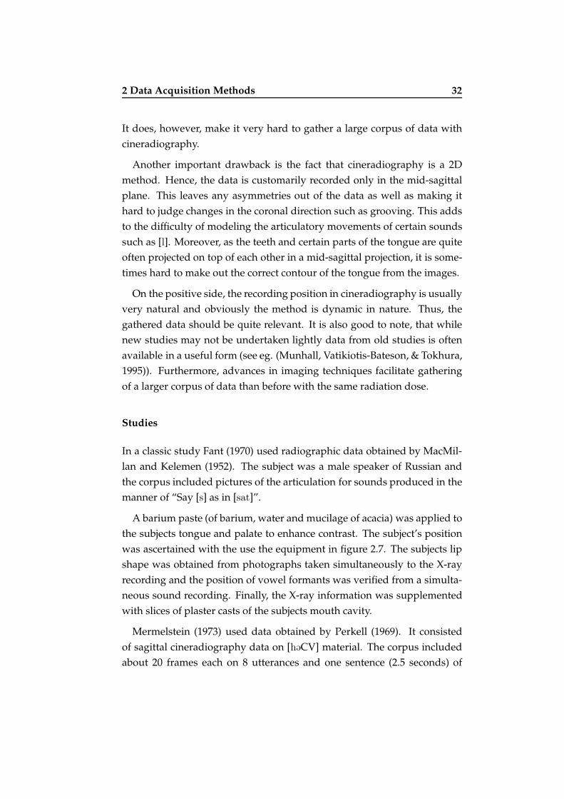
2 Data Acquisition Methods 32
It does, however, make it very hard to gather a large corpus of data with
cineradiography.
Another important drawback is the fact that cineradiography is a 2D
method. Hence, the data is customarily recorded only in the mid-sagittal
plane. This leaves any asymmetries out of the data as well as making it
hard to judge changes in the coronal direction such as grooving. This adds
to the difficulty of modeling the articulatory movements of certain sounds
such as [l]. Moreover, as the teeth and certain parts of the tongue are quite
often projected on top of each other in a mid-sagittal projection, it is some-
times hard to make out the correct contour of the tongue from the images.
On the positive side, the recording position in cineradiography is usually
very natural and obviously the method is dynamic in nature. Thus, the
gathered data should be quite relevant. It is also good to note, that while
new studies may not be undertaken lightly data from old studies is often
available in a useful form (see eg. (Munhall, Vatikiotis-Bateson, & Tokhura,
1995)). Furthermore, advances in imaging techniques facilitate gathering
of a larger corpus of data than before with the same radiation dose.
Studies
In a classic study Fant (1970) used radiographic data obtained by MacMil-
lan and Kelemen (1952). The subject was a male speaker of Russian and
the corpus included pictures of the articulation for sounds produced in the
manner of “Say [s] as in [sat]”.
A barium paste (of barium, water and mucilage of acacia) was applied to
the subjects tongue and palate to enhance contrast. The subject’s position
was ascertained with the use the equipment in figure 2.7. The subjects lip
shape was obtained from photographs taken simultaneously to the X-ray
recording and the position of vowel formants was verified from a simulta-
neous sound recording. Finally, the X-ray information was supplemented
with slices of plaster casts of the subjects mouth cavity.
Mermelstein (1973) used data obtained by Perkell (1969). It consisted
of sagittal cineradiography data on [h@CV] material. The corpus included
about 20 frames each on 8 utterances and one sentence (2.5 seconds) of

2 Data Acquisition Methods 33
Figure 2.7: Equipment used to position a speaker for X-ray (Fant, 1970).
120 frames. This study was one of the first to use a semi-polar grid in
converting the mid-sagittal cross-distance to cross-sectional area.
Gay (1977) studied [CVCVC] material with two male subjects. Gay used
in his study a cinecamera at 60 frames per second and had an X-ray gener-
ator produce 1 ms pulses. In order to enhance the quality of the obtained
data Gay used 2.5 mm lead pellets to tag six points on the lips and the
tongue and an additional reference point on the upper incisors. This ex-
perimental setup has obvious similarities with the X-ray microbeam (see
section 2.2.2, page 35 below) and electromagnetic articulography (see sec-
tion 2.2.3, page 37 below) methods.
Harshman, Ladefoged, and Goldstein (1977) applied PARAFAC analy-
sis (Harsman, 1970) to tongue shape data. The raw data was obtained as
cine-fluorograms (x-rays) of five speakers uttering English vowels. The VT
shapes were then traced from the cine-fluorograms chosen to represent the
vowels. The next step was to fit a reference grid to each speaker and use it
to measure the VT cross-sections at 18 points in the sagittal plain.
Maeda (1990) gathered simultaneous cineradiography, labiofilm and
sound data in a study, which involved two female subjects. The corpus
included ten French sentences. The VT was manually traced from the films
and sampled for analysis with the semipolar grid in figure 2.9 (a). Next
the grid and wall intersections were detected automatically. As a final step
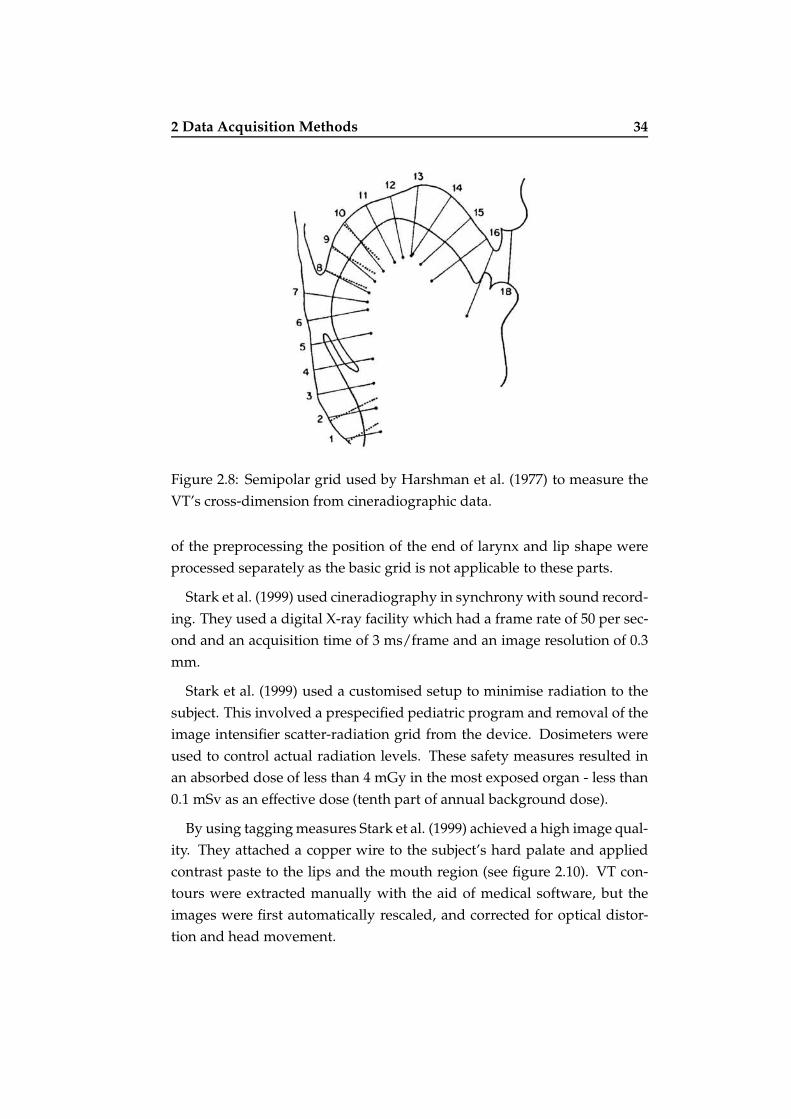
2 Data Acquisition Methods 34
Figure 2.8: Semipolar grid used by Harshman et al. (1977) to measure the
VT’s cross-dimension from cineradiographic data.
of the preprocessing the position of the end of larynx and lip shape were
processed separately as the basic grid is not applicable to these parts.
Stark et al. (1999) used cineradiography in synchrony with sound record-
ing. They used a digital X-ray facility which had a frame rate of 50 per sec-
ond and an acquisition time of 3 ms/frame and an image resolution of 0.3
mm.
Stark et al. (1999) used a customised setup to minimise radiation to the
subject. This involved a prespecified pediatric program and removal of the
image intensifier scatter-radiation grid from the device. Dosimeters were
used to control actual radiation levels. These safety measures resulted in
an absorbed dose of less than 4 mGy in the most exposed organ - less than
0.1 mSv as an effective dose (tenth part of annual background dose).
By using tagging measures Stark et al. (1999) achieved a high image qual-
ity. They attached a copper wire to the subject’s hard palate and applied
contrast paste to the lips and the mouth region (see figure 2.10). VT con-
tours were extracted manually with the aid of medical software, but the
images were first automatically rescaled, and corrected for optical distor-
tion and head movement.

2 Data Acquisition Methods 35
Figure 2.9: Semipolar cineradiography grid (a) and lip measurement points
(b) from Maeda (1990).
In a study resembling that of Maeda (1990), Beautemps et al. (2001)
recorded synchronous cineradiographic labiofilm and sound data. The
corpus included [VCV] (voiced consonants) and [. . . VVV. . . ] material.
Both filming methods had a framerate of 50 images per second.
The X-ray images were first drawn on paper by hand from a projection
and subsequently digitized and split into eleven subcontours. The analysis
was facilitated with the usual semipolar grid (see figure 2.11), which was
extended with dynamical modification possibilities for the lips and larynx
region.
2.2.2 X-ray Microbeam
X-ray microbeam is a point tracking method developed originally by Kir-
itani, Itoh, and Fujimura (1975). It is based on ordinary X-ray technology.
However, instead of imaging the whole VT only small lead or gold pellets
are tracked. The tracking is performed with a very small X-ray beam. The

2 Data Acquisition Methods 36
Figure 2.10: Sample picture with traced VT from Stark et al. (1999) during
articulation of [u].
Figure 2.11: Dynamical semipolar mid-sagittal grid used by Beautemps
et al. (2001) with relevant lip, jaw, tongue, hyoid etc. parameters.

2 Data Acquisition Methods 37
beam’s penetration of the tissues and the pellets is registered with a digital
detector array on the other side of the object as seen in figure 2.12.
Before tracking begins the pellets are first located by scanning the whole
image area. In contrast, during tracking only a neighbourhood around the
pellets’ last locations is sampled. This reduces the amount of radiation
exposure greatly. The only problem with this is that specifically tissues
around the pellet and its projection absorb most of the radiation. Even so,
the amount stays quite small even during a recording of a comparatively
large corpus of data.
The early system had a spatial resolution of 1mm and an effective sample
rate of 100 Hz (Kiritani et al., 1975). The pellet diameter was originally 3
mm, but dropped to 2.5 mm as the material changed from lead to gold
(Fujimura, 1991).
Figure 2.12: X-ray microbeam system diagram (Kiritani et al., 1975).
2.2.3 Electromagnetic Articulography (EMA)
Electromagnetic Articulography is a point tracking method capable of
tracking several tagged points on the face, teeth and tongue of a test sub-
ject. The tracking is based on measuring changing magnetic fields at the
tracked points. The fields are produced by transmitter coils, each of which
has its own field frequency. The position and movement of the tracked
points can be solved by measuring the signals produced by induction in
small receiver coils, which are used to tag the points.

2 Data Acquisition Methods 38
EMA works by estimating from the measured current strength the dis-
tance from the receiver coil to the transmitter coil. The process involves
estimating the local field strength at the receiver from the current strength
and computing the distance thereafter from the field strength. Problems
arise if the estimated field strength is incorrect, which, in turn, is caused by
misalignment of the receiver. To work well, EMA requires that the receiver
and transmitter coil’s main axis be parallel as in figure 2.13. If this is not
the case, the distance will be overestimated.
Figure 2.13: The operation principle of EMA (Perkell et al., 1992). The mag-
netic coupling of two solenoidal coils is illustrated in (a) and (b) shows how
misalignment with the magnetic field effects one winding of a transducer
coil. Here T is the transmitter coil, R the transducer coil, d the distance be-
tween them, Φ the magnetic flux, A the area of a correctly aligned winding,
and θ the angle of misalignment. In (b) the effective area of the misaligned
winding is thus only A cos θ instead of A.
The greatest shortcomings of EMA lie with what can be measured: EMA
is usually confined to the mid-sagittal plane and tracks only points. With
the traditional devices capable of measurement in one plane the method is
also susceptible to error caused by tilting of the receiving coils in relation
to the measurement plane. While the restriction to the mid-sagittal plane is
becoming a thing of the past, EMA is by nature a point-wise measurement
method an this is unlikely to change. Furthermore, the method cannot be
used very deep inside the vocal tract as the coils and wires involved would
trigger the subject’s gag reflex.
Other significant problems are that in order to work the receiver coils
have to be connected with wires to an analysis unit. This means, that when
measuring intra-oral articulation, there will be wires passing into the sub-
ject’s mouth. In addition, the articulation’s naturalness may be affected by
the receiver coils themselves. This is evident from audible deviations on

2 Data Acquisition Methods 39
some sounds, for example [s] (Engwall, personal communication).
Nevertheless, EMA is a very popular method for measuring articulation.
The main causes for its popularity are its safety, its dynamical nature and
the fact that after the initial cost of acquiring the equipment it uses is cheap.
In addition, EMA is well used and hence well understood method with
other less obvious good qualities. For example it can be used simultane-
ously with EPG (see section 2.2.4, page 41 below).
Development of the Method
Probably the first reported attempt to build an EMA device is that of Hixon
(1971). The device worked inversely in comparison to the modern ones:
The magnetic field was generated at the point of interest and measured
with static coils. The coils were very clumsy with a length of 2 cm and
diameter of 5 mm. The device was capable of 1- and 2-dimensional mea-
surements.
In contrast, Lance and van der Giet (1974) reported an experimental
EMA system with two pairs of transmitting static coils and one tracked
receiving coil. The tracked coil in this system was already considerably
smaller with a length 4 mm and a diameter of 2.8 mm. The system was
capable of tracking the position of the receiving coil in real time.
One of the first commercially available systems - called Movetrack - is de-
scribed by Branderud (1985). The dimensions of the transducers (receiving
tracked coils) are 1.5 mm × 4 mm. The two transmitter coils are fixed to a
special helmet. With the original setup the system tracked three transduc-
ers in the mid-sagittal plane, but had a theoretical maximum of 12 trans-
ducers. A Movetrack system used simultaneously with an EPG system can
be seen in figure 2.16, page 43 below.
Perkell et al. (1992) describe two experimental EMA devices: The other
with two transmitters and the other with three. The two experimental de-
vices are evaluated and compared with two commercially available sys-
tems.
The experimental devices took two different approaches in dealing with
the misalignment problem: The three transmitter device used the extra

2 Data Acquisition Methods 40
transmitter’s signal for alignment correction while the two transmitter de-
vice used biaxial receiver coils to actually measure the alignment. The bi-
axial coils consisted of two normal EMA coils mounted at right angles to
each other. In tests the three transmitter was found to be preferable.
The preference was due to a more difficult calibration process, higher
price and higher field strength associated with the two transmitter device.
In general terms the experimental devices had low errors: maximum spa-
tial distortion was 0.5 mm and maximum rotational distortion was less than
0.9 mm for the two transmitter device and less than 2.0 mm for the three
transmitter device. Both devices operated at a sample rate of 100 Hz.
The commercial systems tested by Perkell et al. (1992) were AG100 from
Carstens Medizinelektronik and Movetrack from Special Instrument AB.
Either one was found to be a good choice depending on the choosing cri-
teria: While Movetrack was cheaper, it required more work before it could
be used for experiments as it did not have analysis software bundled with
it.
Recently, an EMA device - called Carstens AG500 - which is not restricted
to the mid-sagittal plane has been in development (Zierdt, Hoole, Honda,
Kaburagi, & Tillman, 2000), (Hoole, Zierdt, & Geng, 2003). Figure 2.14
shows the transmitter coil setup of the system and an actual experimen-
tal situation. With each transmitter transmitting a different frequency the
system is able to track each receiver in 3D and provide two rotational coor-
dinates for them as well.
Figure 2.14: 5D EMA setup: a) schematic picture of the transmitter coil
setup and b) the actual experimental setup. Both from Zierdt et al. (2000).

2 Data Acquisition Methods 41
The prototype is reported to have a spatial resolution which is better than
1 mm and a rotation resolution of about 1◦. The prototype was at first
able to track 4 receiver coils (same as the ones used with Carstens AG100),
and later reported to track 5 (Hoole et al., 2003). As the head moves freely
inside the measurement area, the head position has to be accounted for by
reference coils.
An interesting resource of EMA data - the MOCHA database is de-
scribed by Wrench and Hardcastle (2000). MOCHA (Multi-CHannel Ar-
ticulatory database) contains EMA, EPG and laryngograph data from 40
English speakers reading a maximum of 460 TIMIT sentences. In particu-
lar, MOCHA contains EMA data from the subjets’ lips (two coils), jaw (one
coil), tongue (three coils), and soft palate (one coil). The EMA data has
been recorded at 500 Hz. See section 2.2.4, page 41 for details of the EPG
data.
2.2.4 Electropalatography (EPG)
Electropalatography is a method for dynamically measuring the tongue-
palate contact. The measurement is carried out with a thin artificial palate,
which contains the pressure sensors, that detect tongue contact. The con-
tact pattern can be sampled with a high frequency by attached analysis
equipment. An example of an artificial palate is shown in figure 2.15. (Do
note, that different manufacturers of EPG equipment use different sensor
configurations.)
EPG is limited by the fact, that subjects have to get used to wearing the
artificial palate before reliable measurements can be made. This adds to
the cumbersomeness caused by custom fitting an artificial palate for each
subject - EPG is certainly not a spur-of-the-moment type of investigation
method. In terms of acquired data, EPG is limited only to contact informa-
tion. No information is gained on the tongue-palate distance or movements
of other articulators.
The main good qualities of EPG are its safety and fast sampling rate -
usually either 100 Hz or 200 Hz. The spatial sampling is also quite dense
with electrode numbers ranging from 60 to almost 100. Like EMA, it is also
a well used and well understood method, which produces results, which

2 Data Acquisition Methods 42
Figure 2.15: An artificial EPG palate (produced by Reading) mounted on a
dental cast. (Engwall, 2000c).
facilitate comparison with other studies. Also as mentioned above (see
2.2.4, page 42 for further details) it can be used simultaneously with EMA.
When studying general linguistic phenomena such as coarticulation,
EPG data can be reduced and simplified in many ways (see for example
(Hardcastle, Gibbon, & Nicolaidis, 1991)). In contrast, when using EPG as
a data source for articulatory speech synthesis its greatest value often lies
in fitting artificial contact data from the model with the real EPG data (for
example (Cohen, Beskow, & Massaro, 1998) and (Engwall, 2001b)).
As mentioned above in section 2.2.3 the MOCHA database described by
Wrench and Hardcastle (2000) contains also EPG data. The EPG part of the
database has been recorded with 62 sensor artificial palates with a sampling
frequency of 200 Hz.
Combining EMA with EPG
Simultaneous EMA and EPG recording has been firmly established as a
good method for obtaining dynamic data on articulation (Hoole, Nguyen-
Trong, & Hardcastle, 1993), (Engwall, 2000c), Fuchs and Perrier (1999). The
combination has been found a good match as EMA provides data on the
constriction size and EPG tells whether the situation in the mid-sagittal

2 Data Acquisition Methods 43
plane extends to the sides of the cavity as well. The combination is partic-
ularly useful in studying vowel-consonant coarticulation.
The reservations of both methods have to be taken into account and an
additional consideration is in order when using EMA and EPG concur-
rently (Engwall, 2000c): Even though it is considered quite unlikely, the
data may contain interference from one method to the other. Palate contact
may move the EMA coils or coil contact register as in EPG even if normally
(without simultaneous EMA) no contact would be found. These problems
can be ruled out by separate control registrations with both methods by
themselves.
Figure 2.16: Concurrent recording of EMA and EPG (Engwall, 2000c). The
labels are as follows: X = X-direction transmitter, Y = Y-direction transmit-
ter, H = Head mount, RW = Receiver coil wire, E = EPG unit, EW = EPG
wire, L = Loudspeaker for synchronisation signal, and F = Fastening of
EMA wires with tape.
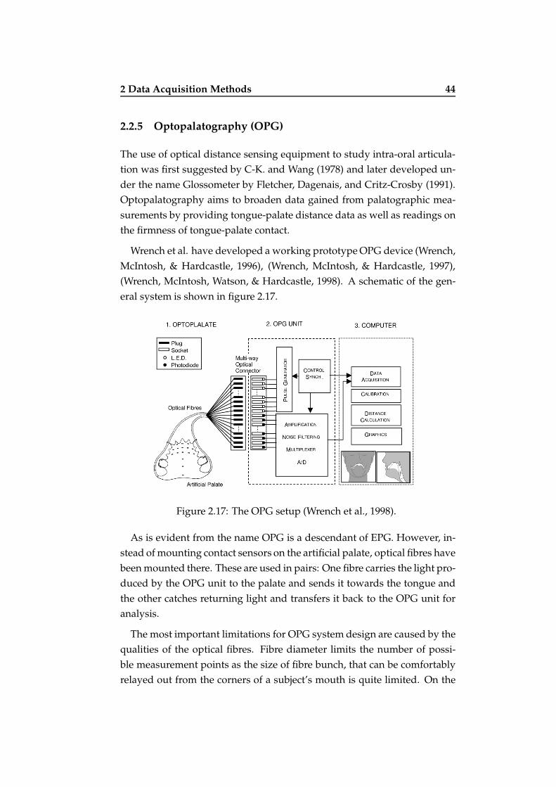
2 Data Acquisition Methods 44
2.2.5 Optopalatography (OPG)
The use of optical distance sensing equipment to study intra-oral articula-
tion was first suggested by C-K. and Wang (1978) and later developed un-
der the name Glossometer by Fletcher, Dagenais, and Critz-Crosby (1991).
Optopalatography aims to broaden data gained from palatographic mea-
surements by providing tongue-palate distance data as well as readings on
the firmness of tongue-palate contact.
Wrench et al. have developed a working prototype OPG device (Wrench,
McIntosh, & Hardcastle, 1996), (Wrench, McIntosh, & Hardcastle, 1997),
(Wrench, McIntosh, Watson, & Hardcastle, 1998). A schematic of the gen-
eral system is shown in figure 2.17.
Figure 2.17: The OPG setup (Wrench et al., 1998).
As is evident from the name OPG is a descendant of EPG. However, in-
stead of mounting contact sensors on the artificial palate, optical fibres have
been mounted there. These are used in pairs: One fibre carries the light pro-
duced by the OPG unit to the palate and sends it towards the tongue and
the other catches returning light and transfers it back to the OPG unit for
analysis.
The most important limitations for OPG system design are caused by the
qualities of the optical fibres. Fibre diameter limits the number of possi-
ble measurement points as the size of fibre bunch, that can be comfortably
relayed out from the corners of a subject’s mouth is quite limited. On the

2 Data Acquisition Methods 45
other hand fibres with a very small diameter can not be used as they have
to be bent 90◦ within the thickness of the artificial palate.
Another important limitation is the signal to noise ratio (SNR). SNR is
affected by light source strength, fibre qualities and possibly by the prox-
imity of the sensor/source pairs in the artificial palate. The proximity prob-
lem can be avoided by operating the points in sequence with only one sen-
sor/source pair active at any given time.
When compared with EPG, OPG has two additional good qualities: It
produces tongue-palate distance measurements and can be used for force
measurements, since all of the light is not actually reflected by the surface
of the tongue, but also from within it. Thus the firmer the contact - and the
greater the force - the stronger the reflection. In addition, when compared
with the Glossometer, OPG clearly facilitates more measurement points.
The latest prototype (Wrench et al., 1998) had 16 sensors built from 0.5
mm plastic optical fibres. The system had a measurement range of 20 mm
and sample rate of 100 Hz. The light sources were infra-red LED sources
and they were used in sequence.
2.2.6 Fast MRI
Fast MRI differs from regular MRI in terms of imaged area and temporal
resolution. The imaged area is always smaller in fast MRI than in static
MRI - usually it is restricted to a single mid-sagittal slice of the VT. With this
reduction comes the advantage of speed: Instead of using several seconds
or even tens of seconds to image the whole VT, one slice can be acquired
in less than a second and with suitable imaging protocols even at rates
approaching 10 Hz. On the other hand by averaging several repetitions
of the same utterance even greater temporal resolution is achievable.
Studies - Real Time MRI
In two similar studies - Demolin et al. (1997) and Demolin et al. (2000) - an
ultrafast implementation of Turbo Spin Echo (TSE) sequence was applied
to achieve MR imaging of the VT with one mid-sagittal, 6 mm thick slice at
4 Hz. The sequence was previously known as TSE Lolo (Local Look), but
currently called TSE Zoom. In the first study the FOV was 300 × 150 mm2

2 Data Acquisition Methods 46
and the pixel matrix 32 × 128 pixels, and in the second study the FOV = 125
× 250 mm2. Figure 2.18 shows two pictures acquired in the second study.
Figure 2.18: Pictures of a male and a female speaker from real time MRI
with grids used in VT cross-dimension measurement.(Demolin et al., 2000).
Recently, Engwall (2004) studied tongue movements with the TSE Zoom
sequence. He was able to acquire one mid-sagittal 6 mm thick slice of the
VT at a rate of 9 Hz. The scanner and equipment were as in (Demolin et al.,
2000), but the pixel matrix size was 128 × 128 and spatial resolution 2.34375
× 2.34375 mm.
Narayanan, Nayak, Lee, Sethy, and Byrd (2004) report a novel approach
to imaging speech production with MRI. They used a spiral sampling strat-
egy in gradient echo imaging. This means that instead of the normal planar
acquisition of images they acquired images in interleaved spirals resulting
in picture as seen in figure 2.19 and, more importantly, a image acquisition
rate of 8-9 fps and a high reconstruction rate of 20-24 fps.
The experiments were carried out with a GE Signa 1.5 T scanner. The
receiver coil was a general purpose head coil. Images were acquired in one
mid-sagittal plane of 5 mm thickness. The resulting effective image resolu-
tion was 2.7 mm with a FOV of 30 cm. Since the study was first with this
imaging sequence, Narayanan et al. (2004) expect to make improvements
with image quality and resolution.

2 Data Acquisition Methods 47
Figure 2.19: A picture from real time spiral echo MRI (Tamil retroflex [í])
(Narayanan et al., 2004).
Studies - Other Fast MRI Methods
As MRI is still a developing method it is probable, that the temporal and
spatial resolution of the scanners and the imaging sequences will continue
to develop further. Furthermore, new imaging methods may well emerge.
Two methods, which have done so, are stroboscopic MRI and tagged MRI.
Mathiak, Klose, Ackerman, Hertrich, Kincses, and Grod (2000) have per-
formed stroboscopic MRI. The principle of stroboscopic MRI is to achieve a
high time resolution by sampling several repetitions of the same utterance.
This obviously requires measures to be taken to ensure that the subject re-
peats the utterance with very little variation between the repetitions and
that, specially, the any movement artefacts are avoided.
The study concentrated on [gVN] material, where the vowel was one of
[o, i, a, e]. Each word had to be repeated 170 times by each of the three
subjects to facilitate reconstruction. The subjects synchronised their pro-
ductions with the imaging sequence by listening to the MRI scanner noise.
The scanner used in the study was a 1.5 T Siemens scanner and the imag-
ing sequence was Fast Low Angle Shot (FLASH). FOV was 200 × 200 mm2
and pixel resolution 256 × 256. With a slice thickness of 8 mm the resulting
voxels were 8 × 0.8 × 0.8 mm3. Only one mid sagittal slice was recorded
during each of the repetitions.
The final temporal resolution of the averaged sequence was 40 Hz, when
the whole mid-sagittal view of the VT was reconstructed. But when only

2 Data Acquisition Methods 48
a section through some important features, such as the uvula, was recon-
structed the temporal resolution reached 120 Hz.
Figure 2.20: Pictures from stroboscopic MRI during the production of [gaN]
(Mathiak et al., 2000). Each of the pictures is a result of averaging over 3
successive frames.
Tagged MRI is another method, which relies on averaging over several
repetitions. It originates from cardiology. Unlike regular MRI, which ex-
cites the imaged tissues evenly, tagged MRI excites the tissues in layers
called tags. As the excited areas then move and deform during movement
of the tissues, a time varying, dynamic sequence can be reconstructed. If
the same utterance is imaged several times, while the direction of tagging
is varied the movement of flesh points inside for example the tongue can
be followed. However, the tags do not last for very long and hence the
utterance length is quite limited.
In an example study by Stone, Dick, Douglas, Davis, and Ozturk (2000),
the tags decayed in 500-600 ms, and thus allowed imaging of quite short
utterances. An example of the resulting images is shown in figure 2.21.
The study consisted of two experiments: The first one aimed at acquiring
data for a 2D tongue model and the second one for a 3D model.
In the first experiment the subject repeated one syllable 32 times. The
imaging was performed in three sagittal planes, which each were 7 mm
thick. The planes had a spatial resolution of 2.4 × 2.4 mm2. 40 tagged
points were tracked.
In the second experiment the subject repeated one syllable 18 times per
slice, which were as follows: 5 sagittal slices repeated with horizontal and
vertical tag planes and 10 axial slices with anterior to posterior tag planes.

2 Data Acquisition Methods 49
The spatial resolution was 1.2 × 2.4 mm2 and slice thickness 7mm. The
resulting sequence had a frame rate of 24 fps (frames per second).
Figure 2.21: Mid-sagittal pictures from tagged MRI (Stone et al., 2000).
The black lines are the tag planes, which have been initially before speech
movements either horizontal (top) or vertical (bottom). Clear internal de-
formations of the tongue are visible in the images in the right side column.
2.2.7 Motion Capture
Motion capture methods are usually based on tracking markers. The mark-
ers are tracked with one or more cameras and so the resulting data de-
scribes the movement of the markers either in two or three spatial dimen-
sions. Because the method does not utilise strong magnetic fields or ionis-
ing radiation, it is completely safe for the subject.
However, some restrictions apply to the quality of data obtained by mo-
tion capture methods. If data from only one camera is available, the result-
ing data is necessarily restricted to two dimensions. Furthermore, as the
system uses either cameras operating in the visible range or in the infrared
range, only visible articulation can be recorded. In marker based systems
the inner lip boundary is a problem, since markers can not be placed there

2 Data Acquisition Methods 50
due to obvious practical problems and problems with naturality of articu-
lation.
On the other hand, motion capture produces data on potentially very
natural articulation as the subject usually sits during recording. Further,
simultaneous intraoral data acquisition is possible. An example can be seen
in figure 2.23.
Studies
In a study by (Honda, Kurita, Kakita, & Maeda, 1995) a general purpose
marker tracking system was used. The left side of the outline of the lips
was tagged with seven markers. These were tracked at a sample rate of 60
Hz with a gray-scale video system the signal of which was automatically
precessed to retrieve the markers’ centroid coordinates. The markers were
hemispherical and had a diameter of 5 mm.
Beautemps et al. (2001) recorded concurrent cineradiography, labiofilm
and sound data. The lips were painted blue and later extracted automat-
ically. The extraction actually yielded the inner contour of the lips as it
was based on the color information rather than the use of markers. The
labiofilm was recorded with one camera at 50 fps (frames per second) with
synchronous sound.
Badin et al. (2002) have recorded video images for motion capture pur-
poses. Figure 2.22 shows examples of the recorded images and the resultant
3D mesh. The system is reported to be cheap to implement in comparison
with commercial motion capture systems.
As seen in the picture the subject’s face was marked with a grid and with
32 plastic beads. Further, his lips were painted blue to facilitate extraction
of lip shape. A side view was provided by a mirror. Thus both the frontal
and side view were recorded with the same camera.
3D coordinates of the 32 flesh markers were extracted by camera per-
spective models, which were calibrated by measuring a know object. In
contrast, the lip shape (as defined by 30 points) was adjusted manually.
Beskow, Engwall, and Granstrom (2003) (see also (Engwall & Beskow,
2003b), (Engwall & Beskow, 2003a)) recorded concurrent EMA (Movetrack)

2 Data Acquisition Methods 51
Figure 2.22: Motion capture with lips painted blue. First image on the left
shows a video image of the subject with a jaw splint, the middle on shows
the lip mesh superposed on the image and the final pair on the right shows
the complete mesh as extracted in 3D from the video images (Badin et al.,
2002).
and motion capture data (Qualisys) with commercial systems. The mea-
surement setup is shown in figure 2.23.
Figure 2.23: Simultaneous EMA and motion capture. Motion capture
marker positions on the left and EMA coil positions on the right (Beskow
et al., 2003).
The recorded material was spoken by one Swedish speaking female sub-
ject in sets of one minute. The material consisted of 270 sentences, 138
[VCV] & [VC1C2{C3}V] words with symmetric vowels and 41 [C1VC2]
words.
The motion capture system used 28 reflective markers (diameter 4 mm)
and four infrared cameras. The markers were positioned on the face and
the Movetrack unit. Furthermore, the lip coil was fitted with one of the
markers. The Movetrack markers and the lip marker were used to align
the data sets. The system extracted the markers’ 3D coordinates at a rate of
60 fps.

2 Data Acquisition Methods 52
In a study comparing slow, normal, rapid and hyperarticulated speech
Maeda and Toda (2003) recorded motion capture data with a Vicon Motion
Capture device. The system used 6 infrared cameras to track 3D coordi-
nates of over 60 markers. The data was recorded at 120 fps.
The recordings were done with one American male and two French fe-
male subjects. Each subject spoke [VCV] nonsense material and a short
text (in English or French according to nationality). The subjects were in-
structed to hyperarticulate the nonsense material and repeat the text with
slow, normal and rapid rate of speech.
2.2.8 Electromyography (EMG)
Electromyography measures electrical potential caused by the contraction
of muscles in response to nerve stimulation. Some examples of EMG data
patterns in relation to the corresponding speech envelope can be seen in
figure 2.24.
Electromyography is performed either with surface electrodes or with
needle electrodes. The needle electrodes are actually thin needles, which
are inserted into the monitored muscle. They are quite uncomfortable. In
contrast, the surface electrodes are often similar to ones used in electrocar-
diography and cause only mild discomfort at most.
Figure 2.24: Examples of EMG data with a corresponding speech envelope.
GGA is anterior part of genioglossus , GGP is posterior part of genioglos-
sus, HG is hyoglossus and SG is styloglossus (Honda, 1996).
However, there is a problem with using surface electrodes. As they are
not very selective the recorded signal may contain interference from other

2 Data Acquisition Methods 53
muscles. On the other hand, needle electrodes are very selective even down
to the level of a few muscle fibres. In other words, if complex muscle groups
are involved it may be necessary to use needle electrodes.
No matter which electrode type is used, recording deep inside the VT
or from intrinsic muscles is very difficult. The restriction on depth of the
recording point inside the VT is caused by the same factors as the same
restriction on EMA. As for the problem with intrinsic muscles, since these
muscles are covered by other muscles surface electrodes are clearly out of
the question, but the possibility of using very long needles is neither a good
solution.
Despite the inherent difficulties with EMG, interesting data on motor
control involved in speech production can be gained from its use. Indeed,
EMG provides very useful data on the physiological mechanisms of speech
production.
Honda et al. (1995) recorded EMG data from muscles, which control lip
movement. Recorded speech material consisted of [ebVbe] and [ewVwe]
sequences where the vowel was one of [i, a, u].
The recording targeted the following lip closing muscles: the orbicularis
oris superior and inferior, the levator anguli oris, the depressor anguli oris,
and the mentalis and the following lip opening muscles: depressor labii
inferioris, and the levator labii superioris.
The data was recorded with two different types of surface electrodes.
The first type was a disc electrode with a diameter between 4 and 6 mm.
These were made from electrocardiography electrode material. The second
type was a miniature cup electrode with Ag-AgCl discs of 2 mm diameter
surrounded by electrode paste.
Hirayama, Vatikiotis-Bateson, and Kawato (1993) recorded EMG data
from eight orofacial and extrinsic tongue muscles controlling jaw and lip
closing and opening and tongue lowering and raising. The recording was
done with surface and hooked-wire electrodes. The recorded material in-
cluded real English speech and nonsense sequences like [asisuseso] where
the consonants [s, t, p] changed place with each other. The recording was
done at a sample rate of 2000 Hz, which was rectified and integrated at 100
Hz to enable its use in a neural network model of articulation.

2 Data Acquisition Methods 54
2.3 Aeroacoustic Measurements
The term aeroacoustic measurements is used here to refer to measuring
air flow and acoustic effects of air flow within the VT. The acoustic effects
of airflow are very minimal in vowel and nasal sound production - if we
consider only the VT and exclude the glottal and subglottal systems. The
situation is quite different during the production of sounds, which rely on
sound being produced in the supraglottal system. The most prominent
example of this class of sounds are the fricative sounds, which are produced
with a noise source provided by turbulent flow through a tight constriction
within the VT. Detailed aeroacoustic studies are necessary to validate and
develop theory on the mechanisms involved.
Airflow can be measured directly both with living subjects and with me-
chanical models. It would obviously be preferable to make all of the mea-
surements within the VTs of real humans, but just as obviously this can
not be done in most cases. Consequently, mechanical models are needed to
enable measurements, which would otherwise be either completely impos-
sible without compromising naturalness of articulation or without compro-
mising the subject’s safety.
Indeed, it is hard to design a setup to measure flow in a fricative con-
striction, without interfering with the articulation. In this light it is not
very surprising that in vivo measurements are usually carried out during
vowel production and more constricted articulations are measured with
mechanical models.
2.3.1 Airflow Measurements with Living Subjects
Teager (1980) analysed the characteristics of airflow in the mouth cavity
during phonation. His instrumentation included three anemometers (hot
wire flow censors) and a microphone. All of these were mounted as an
array. Two of the anemometers were mounted parallel to each other above
the third one. This array was then moved across the mouth during a one
second sustained phonation of [i].
The results were briefly as follows:
2 Data Acquisition Methods 55
1. The sound measurement was more out of phase with the flow mea-
surements (both upper and lower) then is possible to explain by the
construction of the censor array (see figure 2.25).
2. The airflow measurements do not agree with laminar flow. Rather,
they are consistent with separated flows. This means, that instead of
a unified volume flow, there is a different kind of a flow present in
the oral cavity.
3. This seems to mean that sound is actively generated in the mouth
cavity during the described experiment.
Figure 2.25: Flow measurements in the mouth cavity (Teager, 1980).
Anemometers record the local flow velocity very accurately and the di-
rection of the measured flow can be easily controlled (Teager, 1980). There
is, however, one problem with the use of anemometers in speech produc-
tion studies. When recording with a live subject an anemometer can not be
used at positions deep within the VT because of the risk of causing injury
to the subject with the hot wire.

2 Data Acquisition Methods 56
2.3.2 Mechanical Models
Mechanical modeling of articulation is probably the oldest method of
speech synthesis. Over time methods have evolved and currently circuit
models and computational models are more popular. However, in the
context of airflow estimation, mechanical models have recently seen an
increase in popularity. As everything can not be measured with a real
speaker the construction of a more or less flexible mechanical speaker is
often the best alternative.
Studies
Barney, Shadle, and Davies (1999) constructed a Dynamic Mechanical
Model (DMM) of the glottis and the VT. A schematic of the model is
shown in figure 2.26. The DMM consisted of a straight plastic tube of ap-
proximately the same dimensions as a human male VT. At an appropriate
distance from the exit corresponding to the mouth the tube had a pair of
electromechanically driven shutters to act as the vocal folds.
Figure 2.26: Dynamic Mechanical Model of the VT (Barney et al., 1999). The
dimensions are given in centimetres. (The image is not to scale).
Barney et al. (1999) measured the flow field within the DMM with a with
a constant temperature hot wire anemometer inserted through the artificial
tract’s wall. In the measurements they found, that the flow immediately

2 Data Acquisition Methods 57
downstream of the shutters was very irregular. However, by the time the
flow was close to the artificial tract’s exit it had assumed an almost uni-
form cyclic character. This behaviour was considered to be caused by shear
layers forming at the shutter exit with the development of more regular
and even vortices taking place as the flow passes down stream along the
tract. In spite of the fluctuating and, at certain points, irregular nature of
the flow, a mean flow was observed at all measured positions even when
the shutters were closed.
Barney et al. (1999) found that the radiated far-field sound pressure could
be explained only in part by the traditional assumption that the VT acts as a
passive filter for the sound generated at the glottis during phonation. They
had better fit with a model, which included also sound generated by non-
acoustic velocity fluctuation (i.e. vorticity) in the VT.
In the second part of the article Shadle, Barney, and Davies (1999) de-
scribe hot wire anemometer measurements performed in the upper VTs of
four male subjects. The subjects and the recorded speech sound - [2] - were
chosen to correspond closely with the DMM. In addition, the same hot wire
sensors were used as in the DMM measurements.
The hot wire signal was measured with the sensor placed 1 cm behind
the front teeth in the middle of the VT, while the subjects phonated the
vowel [2] for 2 seconds. The signal was sampled at 5 kHz and low-passed
at 2 kHz.
Static flow magnitude and dynamic variation in humans were found to
be similar to the corresponding values in the DMM. Still, the values of the
human subjects were a lot more varied. As the DMM was found to contain
conducting vortices during simulated phonation, the similarity of measure-
ment results was taken as evidence or similar phenomena in the human VT.
Differences in the results were accounted for mainly with several unideal
characteristics of the DMM.
In his Ph.D. thesis Sinder (1999) used a mechanical model, which is
shown in figure 2.27, to validate his fricative production model (see section
4.3, page 103 for more details). The measurement facility consisted of a
straight metal tube, which had cross dimensions of the same order as the
human VT. It had a flow source at one end, feeding a jet flow into the tube.
An obstruction of Gaussian form was placed within the tube at a distance of

2 Data Acquisition Methods 58
5cm (xc in the figure) from the flow source. The flow velocity and average
or time varying pressures could be measured at different points within the
tube by inserting a hot wire anemometer or a pressure transducer through
the wall.
Figure 2.27: A diagram of the flow measurement facility used by Sinder
(1999).
An interesting approach to VT modeling has been taken by Kitamura,
Fujita, Honda, and Nishimoto (2004), who have made resin reconstructions
of the VT based on MRI data. An example is shown in figure 2.28. The
reconstructions are going to be used to measure VT transfer functions for
vowels.
Figure 2.28: A resin reconstruction of the VT based on MRI data (Kitamura
et al., 2004).
2.4 Summary
Several choices of data acquisition methods or combinations thereof can be
argued for quite convincingly. Besides the data collection properties of the

2 Data Acquisition Methods 59
methods factors such as availability and cost of equipment have to be taken
into account. In any case, one of the chosen methods should be a dynamic
one. Furthermore, if the goal is not 2D but 3D synthesis another one should
probably be a static 3D method.
The choice of measurement methods is naturally interconnected with im-
plementation issues of geometric synthesis. These are the topic of the next
chapter.
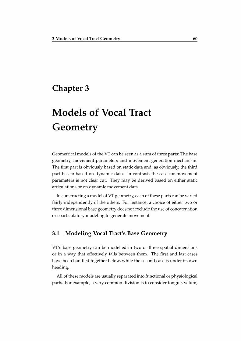
3 Models of Vocal Tract Geometry 60
Chapter 3
Models of Vocal Tract
Geometry
Geometrical models of the VT can be seen as a sum of three parts: The base
geometry, movement parameters and movement generation mechanism.
The first part is obviously based on static data and, as obviously, the third
part has to based on dynamic data. In contrast, the case for movement
parameters is not clear cut. They may be derived based on either static
articulations or on dynamic movement data.
In constructing a model of VT geometry, each of these parts can be varied
fairly independently of the others. For instance, a choice of either two or
three dimensional base geometry does not exclude the use of concatenation
or coarticulatory modeling to generate movement.
3.1 Modeling Vocal Tract’s Base Geometry
VT’s base geometry can be modelled in two or three spatial dimensions
or in a way that effectively falls between them. The first and last cases
have been handled together below, while the second case is under its own
heading.
All of these models are usually separated into functional or physiological
parts. For example, a very common division is to consider tongue, velum,

3 Models of Vocal Tract Geometry 61
jaw, and lips as separate articulators with little or no interaction. Such sep-
aration has the benefits of making the model easier to manage from an
implementation point of view as well as rendering its functioning easier to
interpret in terms of theories of speech production.
3.1.1 Two Dimensional Models
A two dimensional description of VT geometry is required for traditional
source filter methods of speech synthesis with an articulatory model (see
chapter 4). This 2D description is in terms of distance from glottis x and
the cross-sectional area A.
The simplest 2D models of the VT model the cross sectional area A di-
rectly as a function of the distance from glottis x. That is, they are of the
form A(x). A somewhat more complex class of models, model the area as a
function of the mid-sagittal cross-sectional distance d in a piece wise man-
ner. This means, that they define a different area function of the form A(d)
for different regions of the VT.
Furthermore, two parts of the VT are usually modelled separately from
the rest. These parts are the lips and the nasal tract. The separate modeling
of lips follows from the fact that the region of the VT in question changes
not only its area but also its length. In contrast, the nasal tract is considered
a separate part in many models, since it does not change its characteristics
significantly over time, but rather only its coupling with the main tract.
The αβ-model
The most used way to define the relation between the mid-sagittal dimen-
sion of the VT and its cross-sectional area first appears in a paper by Heinz
and Stevens (1964). It has become to be known as the αβ-model after its
parameters. It relates the sagittal cross-sectional distance d to the cross-
sectional area A simply as follows:
A = αdβ (3.1)
Here α and β are parameters, which depend on the position in the VT.
Examples of the use of this model can be found in the next section.

3 Models of Vocal Tract Geometry 62
Models
Lindblom and Sundberg (1971) used a version of the αβ-model with pa-
rameters shown in table 3.1. The model was reported to be inaccurate for
modeling pharyngeal VT area if the cross-sectional distance d exceeds 20
mm, but otherwise achieved reasonable accuracy.
The values for α and β used by Lindblom and Sundberg (1971) are listed
in table 3.1. There are no values for lips because they were modeled sepa-
rately with a different type of model (see section 3.2.2, page 66).
Table 3.1: Values of α and β used by Lindblom and Sundberg (1971)
Region α β
Mouth 2.2 1.38
Upper pharynx 0.68 1.9
Lower pharynx 1.1 2.21
A complex implementation of the αβ-model was used by (Mermelstein,
1973). Mermelstein’s definitions for A(d) are shown in table 3.2. The pha-
ryngeal region follows Heinz and Stevens (1964) while the oral region is an
approximation of data by Ladefoged et al. (1971).
3.1.2 Three Dimensional Models
Modeling the VT as an essentially 2D entity has several problems, which
can be solved by constructing the model as three rather than two dimen-
sional. αβ-type models suffer from a rather complex relationship between
the cross-sectional distance and area and, also, from a need to redefine this
relationship for practically each speaker. In contrast, a 3D model is more
demanding computationally, but gives a very natural way for relating artic-
ulatory movement to changes in the cross-sectional area. Furthermore, it a
3D model is easier to utilise in visual speech synthesis and makes modeling
asymmetric articulation easier.
Like a 2D model a 3D model usually divided into submodels. These can
be, for example tongue, lips, teeth, nasal tract, larynx and the rest of the VT
as one static structure.

3 Models of Vocal Tract Geometry 63
Table 3.2: Definitions of A(d) used by Mermelstein (1973)
Region Formula Note
Pharynx elliptical one axis d and the other
increasing from 1.5 (glot-
tis end) to 3 cm
Soft-palate 2d1.5
Hard-palate 1.6d1.5
Alveolar ridge
to incisors
1.5d,
0.75 + 3(d − 0.5),
5.25 + 5(d − 2),
when d < 0.5
when 0.5 < d < 2
when d > 2
Lips elliptical d is the other axis while
the other = 2+1.5(sl−pl),
where pl is lip protrusion
and sl vertical lip separa-
tion
Several different idealisations can be employed to reduce the model’s
complexity. For example, it can be constructed symmetrically in relation
to the mid-sagittal plane. Further, attached structures can be simplified.
In particular, the nasal cavity can be modelled as a simplified chamber in-
stead of its quite complex structure. Also, piriform sinuses are often either
ignored completely or added to the VT’s cross-sectional area at one or more
points instead of modeling them as small separate branches of the tract.
Even though these models are fully three dimensional volumetric mod-
els, they are usually converted in essence to 2D models when used in sound
synthesis. After the conversion represents the 3D model by an area func-
tion, which simplifies the sound generation process.
Models
Engwall (1999b) (also (Engwall, 1999a)) defined a 3D model of the VT,
which can be seen in figure 3.1. The model is sagittally symmetric. The
model has a static nasal tract, which is modelled simply as one cavity. It
also includes lips, tongue and teeth in the oral region.

3 Models of Vocal Tract Geometry 64
Figure 3.1: A 3D vocal tract by Engwall (1999b). The tongue, teeth and lips
are shown in grayscale and the rest of the vocal and nasal tracts are shown
in wireframe.
Badin et al. (1998) employed a construction method later used also by
Engwall and Badin (1999). Half of a resulting VT is shown in figure 3.2. In
both cases the construction of the model geometry was based on slices of
the VT obtained with MRI.
After VT contour extraction Badin et al. (1998) sampled the contours in
each slice at 51 points. The sample points were organised consistently so
that they could be connected with fibres, which range the whole length of
the VT connecting sample points with the same index in adjacent slices.
Especially, fibres connecting the points 1 and 51 correspond to one side of
the mid-sagittal contour while the fibre connecting point 26 in each slice
corresponds to the other side.

3 Models of Vocal Tract Geometry 65
Figure 3.2: A 3D vocal tract by Badin et al. (1998). The model has been cut
in half along the mid-sagittal fibre. The semipolar grid in the picture is the
grid formed by the original samples.
3.2 Parametrisation of Vocal Tract Movement
Parametrisation of movement is performed in order to reduce complexity
of measurement data and - even more importantly - to gain understand-
ing of its structure. In other words, to understand the process of speech
production.
If sufficient measurement data is available, finding a parametrisation
could be forgone by simply using the raw data as a basis for a concatenation
library. This, however, is usually not desirable because of the prohibitively
large library size. Hence, parametrisation is performed in practically every
study.
The parameters can be defined either based on heuristic decisions, statis-
tical analysis of data or directly on the physiology of the speech production
organs. All of these approaches have in common the use of one or more
data sources, while at the same time using phonetic common sense to keep
the model useful and realistic.

3 Models of Vocal Tract Geometry 66
3.2.1 Physiological Models
In a conceptual sense, the most straightforward way to define the para-
metrisation of speech movements is to use muscles as the basis. However,
it is also a very demanding way to define a model.
At least within the framework of the model it adds a new level with its
own parameters: the muscles themselves. This is caused by the need to
control and model the workings of a single muscle, which is not as simple
a task as it might seem. Another aspect of the complexity is the need for
physical modeling, which generates a heavy computational demand. Still,
these are important models, since through them we can gain knowledge
that might not be as readily available from different types of modeling.
Most of the physiological models discussed in this text have a fairly
strong (or even practically inseparable) connection between movement pa-
rameters and movement generation. Therefore, examples of physiological
models are given later in section 3.3.2, page 80.
3.2.2 Heuristically Defined Models
The term heuristic model is used here to refer to models, which are pri-
marily based on phonetic theory and human anatomy. In particular the
parameters of these models are based on theoretical knowledge rather than
data driven methods such as statistical analysis.
Nevertheless, these models are usually based on measurement data. The
connection comes in the form of activation levels of the parameters, which
are most commonly defined by comparison and/or fitting with measure-
ment data. This approach lessens the possibility of performing unrealis-
tic synthesis, while keeping the model construction relatively simple and
straightforward.
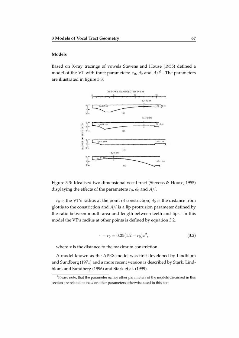
3 Models of Vocal Tract Geometry 67
Models
Based on X-ray tracings of vowels Stevens and House (1955) defined a
model of the VT with three parameters: r0, d0 and A/l1. The parameters
are illustrated in figure 3.3.
Figure 3.3: Idealised two dimensional vocal tract (Stevens & House, 1955)
displaying the effects of the parameters r0, d0 and A/l.
r0 is the VT’s radius at the point of constriction, d0 is the distance from
glottis to the constriction and A/l is a lip protrusion parameter defined by
the ratio between mouth area and length between teeth and lips. In this
model the VT’s radius at other points is defined by equation 3.2.
r − r0 = 0.25(1.2 − r0)x2, (3.2)
where x is the distance to the maximum constriction.
A model known as the APEX model was first developed by Lindblom
and Sundberg (1971) and a more recent version is described by Stark, Lind-
blom, and Sundberg (1996) and Stark et al. (1999).
1Please note, that the parameter d0 nor other parameters of the models discussed in this
section are related to the d or other parameters otherwise used in this text.
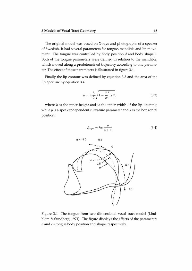
3 Models of Vocal Tract Geometry 68
The original model was based on X-rays and photographs of a speaker
of Swedish. It had several parameters for tongue, mandible and lip move-
ment. The tongue was controlled by body position d and body shape c.
Both of the tongue parameters were defined in relation to the mandible,
which moved along a predetermined trajectory according to one parame-
ter. The effect of these parameters is illustrated in figure 3.4.
Finally the lip contour was defined by equation 3.3 and the area of the
lip aperture by equation 3.4.
y = ±h
2
√
1 −2
w
p
|x|p, (3.3)
where h is the inner height and w the inner width of the lip opening,
while p is a speaker dependent curvature parameter and x is the horizontal
position.
Alips = hwp
p + 1(3.4)
Figure 3.4: The tongue from two dimensional vocal tract model (Lind-
blom & Sundberg, 1971). The figure displays the effects of the parameters
d and c - tongue body position and shape, respectively.

3 Models of Vocal Tract Geometry 69
A more recent version of the same model is described by Stark et al.
(1996) and Stark et al. (1999). The goal of the system is to study apical
sounds (and hence the name). Like the original model it uses the αβ-model
for cross-sectional distance to area conversion.
The model has eight synthesis parameters controlling the submodels.
Lips are included only as an area model and epiglottis and larynx are mod-
eled by translating and rotating static contours. Mandible (teeth and mouth
floor) is modelled as a static contour, which is positioned according to the
mandible parameter.
In contrast, the tongue model includes two more detailed submodels.
Tongue apex is modeled with a parabolic curve between tongue body and
tip and controlled with protrusion and curvature. As the apex-body fit is
kept smooth by rotation the curvature parameter has the effect of lifting the
tongue tip.
The tongue body is controlled with two parameters called position and
deviation. Position is the back-front position and deviation is the degree
of the constriction. The actual tongue hump is produced with a modified
(non-symmetric) Gaussian function.
Mermelstein (1973) developed a VT model based on X-ray data from
Perkell (1969). The a schematic representing the model is shown in figure
3.5. The model’s parameters are also marked in the figure.
The jaw (angle θj and distance sj) and the hyoid bone move in a fixed
coordinate system. The lips and tongue-body move relative to the jaw. The
tongue tip moves in relation to the tongue body and velum opening is con-
trolled in a fixed coordinate system.
Coker (1976) define an articulatory model, which has two separate
speeds for tongue movement (see figure 3.6). This definition is based
on data from Houde (1967). Hence, there are two parameters for slow jaw
and tongue body movements along with one parameter for fast tongue
body movements. These correspond respectively to movement relating to
vowels and consonants.
In addition to the above, there are two parameters for raising and curl-
ing back the tongue tip. Also, the model has a purely acoustical parameter

3 Models of Vocal Tract Geometry 70
Figure 3.5: A two dimensional vocal tract (Mermelstein, 1973) displaying
the effects of the parameters. (See text for explanations.)
Figure 3.6: A two dimensional vocal tract (Coker, 1976) displaying the ef-
fects of the parameters. (See text for explanations.)
for controlling the velar opening and one for controlling constriction in up-
per pharynx. Finally, one parameter is used to limit the smallest possible
according cross-sectional area of the VT according to phonetic context.
A model based on the above Mermelstein model is presented by Rubin,
Baer, and Mermelstein (1981) and Rubin et al. (1996). The latter version is
part of a synthesiser called CASY (Configurable Articulatory SYnthesiser).
Its parameters are shown in figure 3.7 and explained in table 3.3.
An example of a practically non-geometrical articulatory synthesiser can
be found in Stevens and Hanson (2003). Their synthesiser maps articula-
3 Models of Vocal Tract Geometry 71
Figure 3.7: A two dimensional vocal tract (Rubin et al., 1996) displaying the
effects of the parameters. (See text for explanations.)
Table 3.3: Articulatory parameters of CASY (Rubin et al., 1996).
LP lip protrusion
LA lip aperture
TDCL tongue dorsum constrict location
TDCD tongue dorsum constrict degree
LTH lower tooth height
TTCL tongue tip constrict location
TTCD tongue tip constrict degree
TTCO tongue tip constrict orientation
VEL velic aperture
GLO glottal aperture
Ps subglottal pressure
Pt transglottal pressure
∆F0v change in virtual fundamental frequency
tory control parameters directly to the control parameters of a format syn-
thesiser without any geometrical representation at all. However, the pa-
rameters are physiologically motivated. They are shown in table 3.4 and
their relation to VT physiology is illustrated by figure 3.8.
3.2.3 Statistically Defined Models
Liljencrants (1971) analysed mid-sagittal VT shapes with Fourier analy-
sis. While Fourier representation is not very natural for VT, Liljencrants’

3 Models of Vocal Tract Geometry 72
Figure 3.8: a) The relation of HLsyn parameters to VT physiology and b)
the procedure of mapping the pseudo-articulatory parameters to the for-
mant synthesis parameters (Stevens & Hanson, 2003). See table 3.4 for an
explanation of the parameters.
Table 3.4: Articulatory parameters of HLsyn (Stevens & Hanson, 2003).
f1-f4 Formant frequencies F1-F4
f0 Fundamental frequency F0
ag Average area of glottal opening between the mem-
branous portion of the vocal folds
ap Area of the posterior glottal opening
ps Subglottal pressure
al Cross-sectional area of the constriction at the lips
ab Cross-sectional area of tongue blade constriction
an Cross-sectional area of velopharyngeal port
ue Rate of increase of VT volume
dc Change in vocal-fold or wall compliances
work does prove an important point: Two to three parameters or compo-
nents give an accurate description of the mid-sagittal movements of the VT.
Hence, such results from other - more suitable - methods are very natural.
In a certain sense statistical models can be considered the other side of

3 Models of Vocal Tract Geometry 73
the coin when compared with heuristic models. This is because statistical
analysis can be considered most interesting when its results agree closely
with the theory of phonetics. This means that the analysis should produce
parameters, which correspond to traditional classification systems of artic-
ulation and/or speech sounds. When the chosen method does not produce
suitable variables, it has to be forced to do so.
The greatest benefit of using statistical analysis to define the parameters
of a VT model is its direct basis on data. Even if the parameter generation
is forced, it is quite unlikely to produce unnatural results. However, at the
same time the basis in data means, that often quite lengthy processes of
data acquisition, preparation and analysis are needed.
Parallel Factorial Analysis (PARAFAC)
PARAFAC is described in Harsman (1970). It is a variant of factorial anal-
ysis, which does not require the factors or parameters to be uncorrelated.
With this concession comes the benefit of having a unique solution for the
problem of fitting the model to a given data set.
Figure 3.9: The effect of parameters t1 (front-raising) and t2 (back-raising)
extracted from X-ray data with PARAFAC (Ladefoged et al., 1978).
Ladefoged et al. (1978) used three way factor analysis (also known as
three way component analysis) to obtain components of tongue movement
in the sagittal plain. The procedure is described in in (Harshman et al.,
1977) (see also section 2.2.1, page 31). The effect of varying the resulting
parameters can be seen in figure 3.9. They correspond - without forced
analysis - to front-raising and back-raising of the tongue.

3 Models of Vocal Tract Geometry 74
While PARAFAC is usually quite successful with mid-sagittal data, this
is not always the case as reported by Zheng and Hasegawa-Johnson (2003).
In addition they report, that when applied to 3D data PARAFAC is able
to extract parameters, which correspond to the parameters, that it extracts
from the mid-sagittal portion of the same data. In contrast, lateral effects
are not represented so well by the results of PARAFAC analysis.
Factor Analysis 2
Factor analysis is a method for dimensional reduction of data which are
considered to follow a multidimensional normal distribution. In matrix
form the factor model can be written as:
x = µ + Af + u, (3.5)
where x is an original observation vector, µ the expected value vector of
the observed phenomenon, A the loading matrix, and f and u two inde-
pendent random variables.
Factor analysis can be applied as a kind of forced version, where certain
interesting components are first extracted from the data by linear regression
analysis. After this the remaining variance is analysed with normal factor
analysis methods. This type of analysis is called arbitrary factor analysis
(here AFA) (Maeda, 1990).
Maeda has used AFA to analyse VT shapes in two studies (Maeda, 1979)
and (Maeda, 1990). The first study was based on data from one female
speaker and concentrated on analysing only the tongue shape.
The second study used data from two speakers - one male and one fe-
male. The tongue parameters extracted for one of the speakers of the study
are shown in figure 3.10. The study included also similar analysis of the
lips, larynx and velum as independent parts of the resulting model. This
2Please note, that the division to factor analysis and principal component analysis re-
flects the terminology used by the original authors. From a statistician’s point of view the
terms would be almost interchangeable here. This comes from the fact, that the essential
difference is whether the analysed data is considered to be multinormally distributed or
not.

3 Models of Vocal Tract Geometry 75
Figure 3.10: The effects and explained variances of four parameters ex-
tracted from X-ray data with AFA by Maeda (1990).
separate analysis and parametrisation was based on the assumption, that
physiologically separate articulators should be separated also in the model.
Principal Component Analysis (PCA)
PCA is a method for dimensional reduction of data. Unlike factor analysis
the data need not be considered to follow a multidimensional normal dis-
tribution. However, like factor analysis, principal component analysis is
commonly applied in either a guided or a forced form when used on artic-
ulatory data. In the forced form it is often called linear component analysis
(LCA).
Two dimensional tongue parameters resulting from PCA were used by
Kaburagi and Honda (1996). While the analysis of the tongue movement
itself was unforced, the effect of jaw movement was first removed from the
EMA data. Resulting parameters can be seen in figure 3.11. They explained
97% of the variance.
Badin et al. (1998) used guided PCA to analyse MRI data. The method in-
volves iterative application of PCA to the remaining variance. At each step

3 Models of Vocal Tract Geometry 76
Figure 3.11: Tongue parameters derived with PCA from EMA data
(Kaburagi & Honda, 1996). The crosses represent the movement of the
EMA measurement coils and the solid lines the effect of the principal com-
ponents.
one or two principal components are chosen based and subtracted from the
data. The choice is based on clear interpretability of the components rather
than on the amount of explained variance. The authors report, that this
procedure does not result in the greatest possible explanation of variance,
but does often yield components, which can be easily interpreted.
Figure 3.12: Nomograms for 3D VT parameters by Badin et al. (1998). The
parameters shown here were given names as follows: JH = jaw height, TB
= tongue body, TD = tongue dorsum, and TT = tongue tip.

3 Models of Vocal Tract Geometry 77
Badin et al. (1998) extracted five components, which could be given an in-
terpretation and four more, which could not. Four of the first five are illus-
trated in figure 3.12. The remaining named component, which is not shown
in 3.12 was TA = tongue advance. The named components explained 75 %
of the variance, and when four more components were added with classical
(unguided) PCA, the whole model explained 94 % of the variance.
Engwall (2000a) constructed a 3D tongue model, which was based on an
earlier mid-sagittal (2D) VT model (Engwall & Badin, 1999). While the 2D
model was defined by guided PCA (see above the study by Badin and also
(Beautemps et al., 2001)), the 3D model was defined with LCA. The first five
parameters of the 3D model were chosen to correspond to the parameters
of the 2D model. A sixth parameter was then added based on the remaining
variance. The effect of these parameters can be seen in figure 3.13.
Figure 3.13: Nomograms for 3D tongue parameters by Engwall (2000a).
The names of the parameters are: JH = jaw height, TB = tongue body, TD =
tongue dorsum, TT = tongue tip, TA = tongue advance, and TW = tongue
widening.
Four parameters of the original 2D mid-sagittal model achieved an ex-

3 Models of Vocal Tract Geometry 78
plained variance of 90 %. In contrast, the first five components of the 3D
model achieved on sagittal data an overall explained variance of 78 % and
a mid-sagittal explanation ratio of 88 %.
Badin et al. (2002) developed a 3D tongue model in a similar manner
as the one by Engwall above. However, its basis was a 2D tongue model,
which was extracted from the mid-sagittal portion of the same data set with
LCA. The resulting 3D model thus had the same five parameters as the 2D
model. Three of these are illustrated in figure 3.14. The explained variances
for the 3D model were 72 % of the total variance and 89 % of the mid-
sagittal variance.
Figure 3.14: Nomograms for three of the 3D tongue parameters by Badin
et al. (2002). The parameters shown here were named JH = jaw height, TB
= tongue body, TD = tongue dorsum.
3.3 Movement Generation
When a suitable parametrisation of VT movement and a phonetic descrip-
tion of the speech material to be synthesised are available, movement can

3 Models of Vocal Tract Geometry 79
be generated. This can be achieved with either heuristic rules, concatena-
tion, muscle modeling, coarticulatory modeling, gestural modeling or in
some other way.
3.3.1 Heuristic Movement Models
In comparison with defining movement parametrisation, defining a move-
ment generation mechanism can be quite hard, if there is no relevant data
available. This is due to the fairly complex way, that our articulatory or-
gans move. However, if some sort of data is available, a heuristic approach
is probably one of the easiest to implement as one gets to decide the types
of functions used et cetera without any restrictions. Thus, heuristic mod-
els of movement generation rely on observation based rules to produce the
movement trajectories.
Models
Mermelstein (1973) defined a dynamic articulatory model. It synthesised
[VCV] -sequences by generating movement trajectories for the static artic-
ulatory model discussed in the same article.
The dynamic model was based on the following principles: Vowel move-
ment is slow and precise while stop release involves a fast articulator move-
ment. Stationary vowels require four parameters (out of nine defined in the
mid-sagittal articulatory model). These were two tongue body position,
one jaw, and one lip position parameters. In addition to these consonants
need also tongue tip, lip height, and velar opening parameters. Consonant
synthesis poses restraints only on certain parameters and instead of defin-
ing absolute values defines only parameter space regions which should be
reached. In addition, some parameters are not restrained by consonants at
all.
The varying effect of consonants on different parameters was achieved
by defining a pertinence rank for the parameters in different types of conso-
nant productions. For example tongue body parameters were given a rank
of 1 for velars (condition has to be met), a rank of 2 for alveolars (parameter
has to be within a given range) and a rank of 3 for labials (no restrictions).

3 Models of Vocal Tract Geometry 80
The model also contained detailed rules for articulator activation. These
were based on observations on [h@CV] material. In particular, timing events
were fixed at the values observed in the data. In contrast, the amplitude of
activation and F0 contour were determined in an ad hoc manner.
3.3.2 Physiological Models
Generating movement with a physiological model can be quite complex, if
the model mirrors the physiology very closely. This fact becomes evident,
when one notes, that for such a model the parameters should be artificial
neural signals, which cause artificial muscles to contract. The generation
of the neural signals for a given utterance is made harder by the problems
faced in recording such signals (see section 2.2.8, page 52 for more details).
The task of synthesis can be simplified a bit by resynthesising an utter-
ance from EMG data and thus skipping the need to generate the control
signals. Even so, the model will not be a simple one as muscle physics are
very complex and not yet anywhere close to being a routine task.
As mentioned previously (see section 3.2.1, page 66), the models are de-
scribed below not only in relation to movement generation, but also in re-
lation to movement parametrisation.
Models
Honda (1996) has developed a 2D physiological model of the VT. The
model includes the tongue, jaw, hyoid bone, laryngeal cartilages and, the
vocal folds. These organs are moved in the model by 21 active muscles. In
the case of rigid bodies the physics are modeled with mass-spring systems
while the tongue’s deformations are calculated with a finite element model
(FEM).
In the model the motor organisation of the tongue is modeled as three
layers: First, the peripheral mechanics or muscle physics, second, motor
command generation and, third, sensorimotor integration. The model’s
musculature for controlling tongue movement consists of four extrinsic
muscles. These are organised into two opposing muscle pairs, which are
genioglossus posterior vs. hyoglossus and styloglossus vs. genioglossus
anterior. These pairs and their effect on the tongue are shown in figure 3.15

3 Models of Vocal Tract Geometry 81
Figure 3.15: Tongue model based on extrinsic muscles (Honda, 1996). The
effects of two opposing muscle pairs are illustrated.
Honda (1996) found the muscle pair model to be consistent with the sta-
tistical parameters of Maeda (1990). Additionally, the two pairs formed an
orthogonal space, which enabled synthesis of tongue movements. Honda
(1996) used an ensemble of average EMG waveforms as input for the
model. As seen in figure 3.16, these were plotted as a vector sum, which
was then used as the activating force.
Payan and Perrier (1997) have created a physiological tongue model.
Like the above Honda’s model it uses FEM for modeling tongue deforma-
tion, but unlike Honda’s work it implements the equilibrium point hypoth-
esis (Feldman, 1966). The hypothesis states, that the central nervous system
controls a threshold muscle length. Furthermore, motorneurons integrate
the proprioceptive feedback and the current threshold length to a possi-
ble activation of muscle contraction. To produce continuous movement the
central nervous system sets a discrete sequence of threshold length values,
which are interpolated linearly between the start and end values.
Payan and Perrier (1997) implemented the muscles seen in figure 3.17.
Muscle activation was modeled as force effects on mesh nodes correspond-
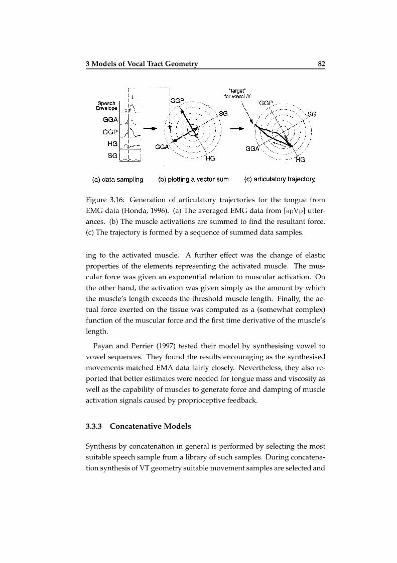
3 Models of Vocal Tract Geometry 82
Figure 3.16: Generation of articulatory trajectories for the tongue from
EMG data (Honda, 1996). (a) The averaged EMG data from [@pVp] utter-
ances. (b) The muscle activations are summed to find the resultant force.
(c) The trajectory is formed by a sequence of summed data samples.
ing to the activated muscle. A further effect was the change of elastic
properties of the elements representing the activated muscle. The mus-
cular force was given an exponential relation to muscular activation. On
the other hand, the activation was given simply as the amount by which
the muscle’s length exceeds the threshold muscle length. Finally, the ac-
tual force exerted on the tissue was computed as a (somewhat complex)
function of the muscular force and the first time derivative of the muscle’s
length.
Payan and Perrier (1997) tested their model by synthesising vowel to
vowel sequences. They found the results encouraging as the synthesised
movements matched EMA data fairly closely. Nevertheless, they also re-
ported that better estimates were needed for tongue mass and viscosity as
well as the capability of muscles to generate force and damping of muscle
activation signals caused by proprioceptive feedback.
3.3.3 Concatenative Models
Synthesis by concatenation in general is performed by selecting the most
suitable speech sample from a library of such samples. During concatena-
tion synthesis of VT geometry suitable movement samples are selected and

3 Models of Vocal Tract Geometry 83
Figure 3.17: The bold lines represent orientation and points affected by
muscle forces in a FEM model by (Payan & Perrier, 1997). Further, the gray
areas represent elements, which change their elastic properties when the
muscle is activated.
possibly filtered to form the desired articulatory movements. This is analo-
gous with concatenative sound synthesis, where sound samples are treated
in much the same way. Another analogy is the most commonly used sam-
ple unit, which for sound synthesis is the diphone and for articulatory syn-
thesis the diart. Both correspond to a segment from the stationary part of
one phoneme or articulation to the stationary part of the next phoneme or
articulation.
Segmenting the data poses some problems as the stationary part of a
phoneme or articulation is not always very clearly defined. However, the
most difficult tasks in this type of synthesis are the construction of the sam-
3 Models of Vocal Tract Geometry 84
ple library and the selection of the most suitable sample to be used in a
given context.
The samples may be either raw unprocessed data or, for example,
parametrised data. The latter approach gives the benefit of reducing the
library size, which can easily be very large.
Models
Greenwood (1997) describes the process of building a articulatory synthe-
siser utilising concatenation of diarts. The samples were generated from
MRI data, which was simplified to provide only the area functions along
with the corresponding formants as the aim was spectral copy synthesis.
Rather than use a single monolithic codebook or library Greenwood
(1997) generated several separate ones. Each of these corresponded to a
voiced diphone. Also, the method of finding the best sample from the
library was enhanced by using a two component cost function. It took into
account not only the formants, but also the changes in area functions from
frame to frame.
To reduce the complexity of the data, Greenwood (1997) parametrised
the MRI data. Two different parametrisations were used and compared
with each other. One was a descendant of Mermelstein’s model (Mer-
melstein, 1973) and the other was quasi articulatory model (Greenwood &
Goodyear, 1994). As the synthesis results were compared little difference
was found between the two systems.
Engwall (2002) presents a concatenative synthesis system capable of
generating a visual representation of articulation. The system concate-
nates diart samples of articulatory parameter transitions. The diart library
was based on data from the MOCHA database (Wrench & Hardcastle,
2000), which was parametrised by fitting it to a 3D tongue model (Engwall,
2000a). After parametrisation the data was segmented into diarts according
to the segmentation used in the MOCHA database.
Timing and phoneme information was produced with Festival (Black &
Taylor, 1997). Selecting diarts from the library was performed by minimis-
ing the cost function:

3 Models of Vocal Tract Geometry 85
C =
5∑
j=1
N∑
i=1
((P s
j (i)− P ej (i− 1)
)2+ wd
(P ′
sj(i)− P ′
ej(i− 1)
)2)
+ wt
N∑
i=1
∆ti,
where Pj are the articulatory parameters, P ′j their derivatives, P sj (i) the
start value of diart i, P ej (i− 1) the end value of diart i− 1. Further, N is the
number of diarts in the utterance, ∆ti the difference between the duration
of diart i and a target duration, and finally wd and wt are weights used to
tune the cost function.
The results were evaluated against the original data from the MOCHA
database as well as X-ray films of other speakers (from the database de-
scribed by Munhall et al. (1995)). The model achieved a good fit in general,
but had problems with underrepresented units. In addition, the move-
ments of tongue tip and root were found too restricted.
3.3.4 Coarticulatory Models
Coarticulation means the effect that the phonemic context (preceding and
following phones) has on the articulation of a given phone. The possi-
ble model types reported in the literature before the early 90’s range from
look-ahead type of models (Öhman, 1967) and time invariant models (Bell-
Berti & Harris, 1982) to hybrid models combining the two (Al-Bamerni &
Bladon, 1982). The first type lets the beginning of a movement toward a
certain articulatory position vary according to the phonemic context while
the second type assumes a fixed onset time in relation to the achievement
of the desired position.
Coarticulatory models have the advantage of providing an interface for
testing theories of dynamic speech production. Indeed, the fact alone, that
a separate algorithmic module for producing articulatory trajectories ex-
ists, makes it possible to try different strategies in the production. On the
other hand, dynamic speech is far from a simple phenomenon. Accord-
ingly, models of coarticulation tend to reflect this. In other words, they
may be quite intricate.

3 Models of Vocal Tract Geometry 86
Models
Cohen and Massaro (1993) defined a model of coarticulation for their visual
speech synthesis system. They used dominance (weighing) and blending
functions in their model. The dominance functions were of the form:
D(t) = αe−θ←|t−t0|c , when t − t0 ≥ 0 (3.6)
D(t) = αe−θ→|t−t0|c , when t − t0 < 0 (3.7)
Here D(t) is the either the anticipatory (3.6) or following (3.7) dominance
as defined for a given parameter in a certain segment. Furthermore, the
activation amplitude α and the rate parameters θ← and θ→ are also defined
individually for each of the articulatory parameters and segments. Finally,
t − t0 is the temporal distance from the peak of dominance and c a form
parameter.
The different target values Tsp for each segment s and parameter p were
combined by using a weighted sum at each point in time t:
Fp(t) =
∑Ns=1(Dsp(t) × Tsp)∑N
s=1 Dsp(t)(3.8)
An example of how the model was applied to visual synthesis is shown
in figure 3.18. The model was fitted to the individual phones manually.
Le Goff (1997) (also (Le Goff & Benoît, 1997)) extended the above defini-
tion of D(t) to so as to make it a Cn function (a function with n continuous
derivatives). This extended version is given below as equation 3.9 and ex-
amples are shown in figure 3.19.
D(t) = αe−θi|t−t0| ×
n−1∑
j=0
θji
j!× |t − t0|
j (3.9)
As can be seen the form parameter c is not present. The sum and the
last term provide the necessary smoothing for the n-continuity at the point
where the rate term θi changes.
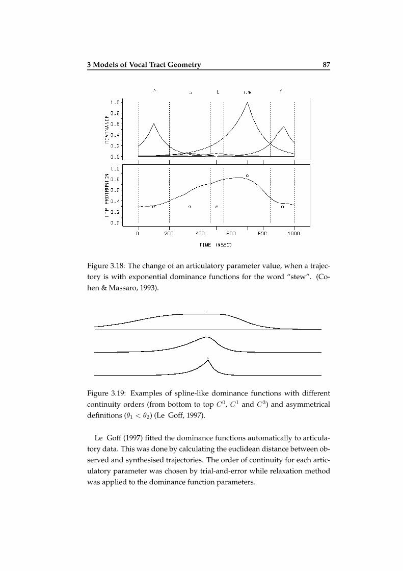
3 Models of Vocal Tract Geometry 87
Figure 3.18: The change of an articulatory parameter value, when a trajec-
tory is with exponential dominance functions for the word “stew”. (Co-
hen & Massaro, 1993).
Figure 3.19: Examples of spline-like dominance functions with different
continuity orders (from bottom to top C0, C1 and C3) and asymmetrical
definitions (θ1 < θ2) (Le Goff, 1997).
Le Goff (1997) fitted the dominance functions automatically to articula-
tory data. This was done by calculating the euclidean distance between ob-
served and synthesised trajectories. The order of continuity for each artic-
ulatory parameter was chosen by trial-and-error while relaxation method
was applied to the dominance function parameters.
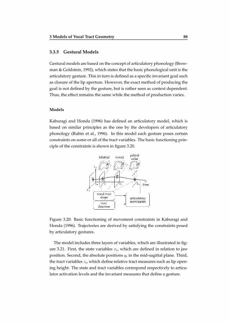
3 Models of Vocal Tract Geometry 88
3.3.5 Gestural Models
Gestural models are based on the concept of articulatory phonology (Brow-
man & Goldstein, 1992), which states that the basic phonological unit is the
articulatory gesture. This in turn is defined as a specific invariant goal such
as closure of the lip aperture. However, the exact method of producing the
goal is not defined by the gesture, but is rather seen as context dependent.
Thus, the effect remains the same while the method of production varies.
Models
Kaburagi and Honda (1996) has defined an articulatory model, which is
based on similar principles as the one by the developers of articulatory
phonology (Rubin et al., 1996). In this model each gesture poses certain
constraints on some or all of the tract variables. The basic functioning prin-
ciple of the constraints is shown in figure 3.20.
Figure 3.20: Basic functioning of movement constraints in Kaburagi and
Honda (1996). Trajectories are derived by satisfying the constraints posed
by articulatory gestures.
The model includes three layers of variables, which are illustrated in fig-
ure 3.21. First, the state variables xi, which are defined in relation to jaw
position. Second, the absolute positions yi in the mid-sagittal plane. Third,
the tract variables zi, which define relative tract measures such as lip open-
ing height. The state and tract variables correspond respectively to articu-
lator activation levels and the invariant measures that define a gesture.
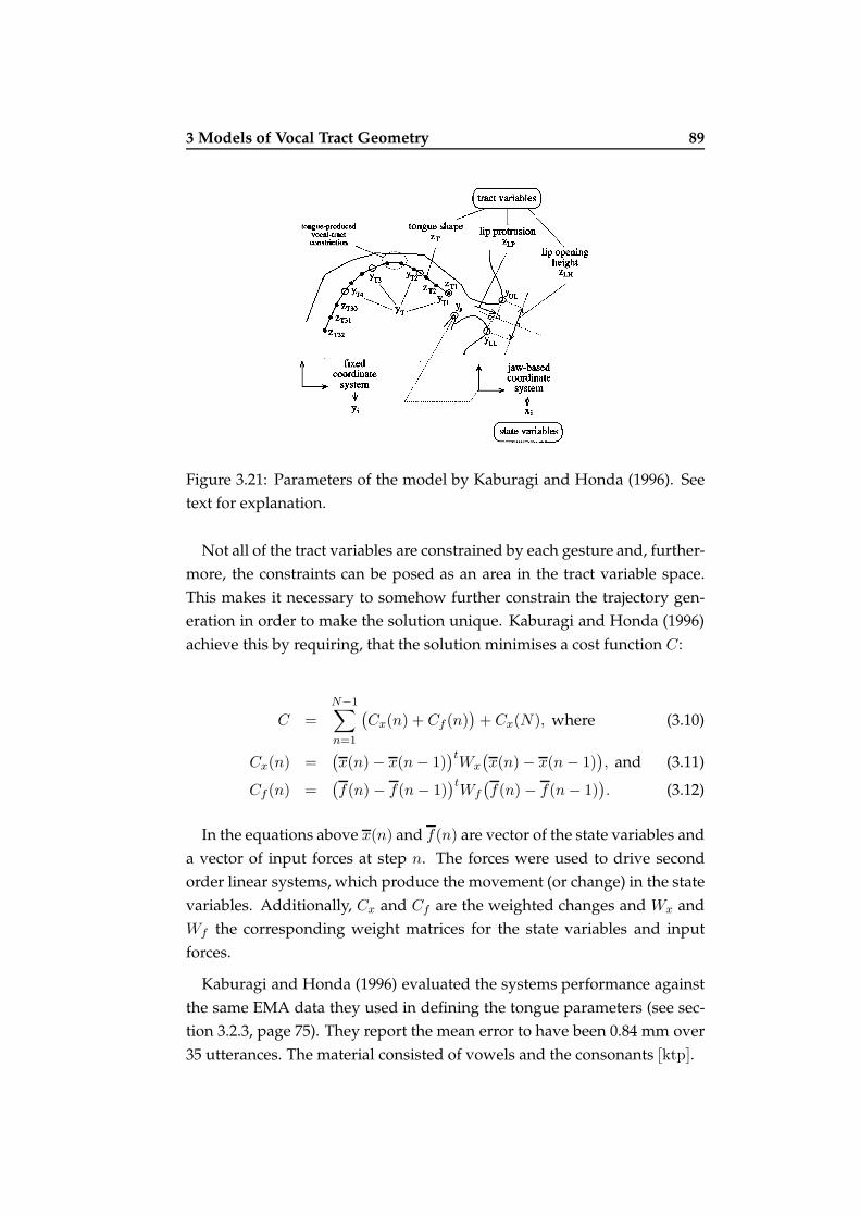
3 Models of Vocal Tract Geometry 89
Figure 3.21: Parameters of the model by Kaburagi and Honda (1996). See
text for explanation.
Not all of the tract variables are constrained by each gesture and, further-
more, the constraints can be posed as an area in the tract variable space.
This makes it necessary to somehow further constrain the trajectory gen-
eration in order to make the solution unique. Kaburagi and Honda (1996)
achieve this by requiring, that the solution minimises a cost function C :
C =
N−1∑
n=1
(Cx(n) + Cf (n)
)+ Cx(N), where (3.10)
Cx(n) =(x(n) − x(n − 1)
)tWx
(x(n) − x(n − 1)
), and (3.11)
Cf (n) =(f(n) − f(n − 1)
)tWf
(f(n) − f(n − 1)
). (3.12)
In the equations above x(n) and f(n) are vector of the state variables and
a vector of input forces at step n. The forces were used to drive second
order linear systems, which produce the movement (or change) in the state
variables. Additionally, Cx and Cf are the weighted changes and Wx and
Wf the corresponding weight matrices for the state variables and input
forces.
Kaburagi and Honda (1996) evaluated the systems performance against
the same EMA data they used in defining the tongue parameters (see sec-
tion 3.2.3, page 75). They report the mean error to have been 0.84 mm over
35 utterances. The material consisted of vowels and the consonants [ktp].

3 Models of Vocal Tract Geometry 90
3.4 Handling Collisions
As a model’s articulators move during speech it becomes necessary to en-
sure, that they do not reach physically impossible configurations. In other
words, collisions have to be handled in some way.
Regardless of the dimensionality of the model, two different approaches
present themselves readily: First, the collisions can be prevented by ensur-
ing that impossible configurations are just that - impossible. The move-
ment parameters can be defined relative to other parts of VT physiology.
For example “move the tongue tip 95% of the way towards the upper in-
cisors”. Second, the collisions can be corrected after they happen. This
means, that after each step of movement generation collisions are detected
and corrected.
The first approach has the desirable property of high computational effi-
ciency at run time. However, the second approach can be said to generate
more realistic results. This is because the second approach provides a pos-
sibility to determine the force used to press the tongue against the palate.
This in turn enables natural deforming of the tongue in such a situations.
Models
Cohen et al. (1998) used the measure: n · P to detect collisions between the
palate and the tongue. Here n is the palate’s surface normal and P a vector
from a tongue point to a palate surface point. Naturally, the collisions can
be detected by examining the sign of the product.
As a way of correcting a detected collision, Cohen et al. (1998) considered
using a parallel projection to move the offending tongue points back to the
palate’s surface. Unfortunately, this strategy can result in undesirable point
distributions as the convex palate surface will produce clustering. Besides,
the method is also fairly slow.
Among other enhancements of the correction process Cohen et al. (1998)
divided the space around the palate and teeth into voxels as illustrated in
figure 3.22. These were assigned a status according to whether a tongue
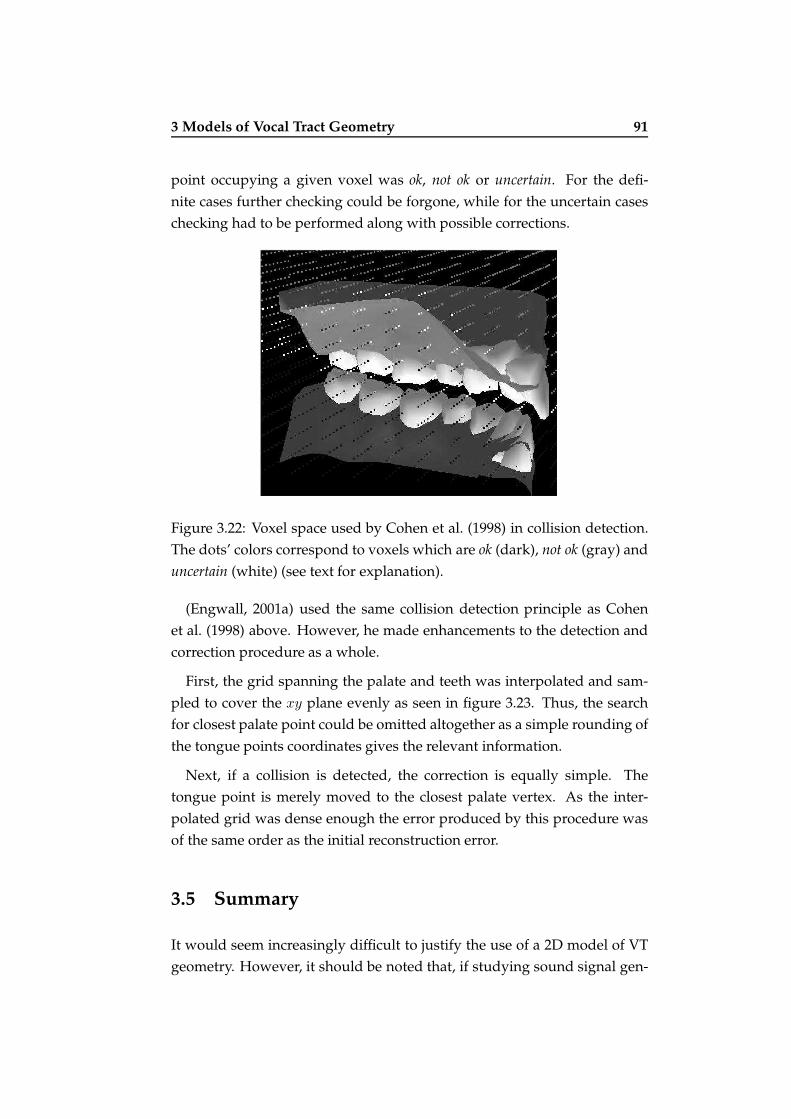
3 Models of Vocal Tract Geometry 91
point occupying a given voxel was ok, not ok or uncertain. For the defi-
nite cases further checking could be forgone, while for the uncertain cases
checking had to be performed along with possible corrections.
Figure 3.22: Voxel space used by Cohen et al. (1998) in collision detection.
The dots’ colors correspond to voxels which are ok (dark), not ok (gray) and
uncertain (white) (see text for explanation).
(Engwall, 2001a) used the same collision detection principle as Cohen
et al. (1998) above. However, he made enhancements to the detection and
correction procedure as a whole.
First, the grid spanning the palate and teeth was interpolated and sam-
pled to cover the xy plane evenly as seen in figure 3.23. Thus, the search
for closest palate point could be omitted altogether as a simple rounding of
the tongue points coordinates gives the relevant information.
Next, if a collision is detected, the correction is equally simple. The
tongue point is merely moved to the closest palate vertex. As the inter-
polated grid was dense enough the error produced by this procedure was
of the same order as the initial reconstruction error.
3.5 Summary
It would seem increasingly difficult to justify the use of a 2D model of VT
geometry. However, it should be noted that, if studying sound signal gen-

3 Models of Vocal Tract Geometry 92
Figure 3.23: The more evenly spaced black mesh has been created by inter-
polating and sampling of the bright mesh. The black mesh makes collision
detection simpler (Engwall, 2001a).
eration is not a central issue in the study, the dimensionality of the model
may be chosen quite freely.
Accordingly, while the idea of using area functions for modeling VT ge-
ometry is by no means new, it is still of central importance. And as we shall
see in the next chapter most of speech signal generation methods utilise
area functions.

4 Acoustic Synthesis 93
Chapter 4
Acoustic Synthesis
With the geometrical data available from one of the models described in the
previous chapter, we get to the final stage in articulatory speech synthesis.
Acoustic synthesis in the context of an articulatory speech synthesiser can
be implemented in several different ways with very varied requirements
and computational loads.
Stark et al. (1996) and (Stevens & Hanson, 2003) (see figure 3.8, page 72)
do it by controlling a formant synthesiser. But as the focus of this thesis is
on simulating the speech production process more interesting methods are:
filter models (electrical circuit analogs as well as computational models)
and models with actual turbulence modeling.
Depending on the geometrical description’s level of detail, some meth-
ods of acoustic synthesis may not feasible. Additionally, not all of the meth-
ods described here are readily able to support synthesis of dynamic speech.
4.1 Mathematical Basis of Modeling Vocal Tract
Acoustics
Before looking at examples of acoustic synthesis systems, it is necessary to
understand some of the mathematics involved in their design. Therefore,
we will derive some basic equations for sound pressure within the VT and
also a more specialised version known as Webster’s horn equation. Subse-
quently, we will review a traditional tube approximation used to solve the
4 Acoustic Synthesis 94
relevant equations. Finally, the source filter model of speech production
will be shortly reviewed.
4.1.1 Basic Equations
To describe wave propagation within the VT mathematically, we need the
definitions given in table A.1 in appendix A. As a first step of our analysis
we will simplify two basic equations by taking certain facts into considera-
tion.
We will begin with a slightly modified form of the law of mass preserva-
tion (4.1) and Euler’s equation (without mass sources) (4.2):
∂p
∂t+ ρ0c
2∇u = 0 (4.1)
ρ0u
∂t+ ∇p = 0. (4.2)
Now, since the frequency range of interest (roughly from 100 to 3000 Hz)
is fairly low in comparison with the frequencies of cross-mode resonances
(lowest is around 10000 Hz for an average male VT), one can assume that
the signal propagates as a plane wave. Therefore, the equations 4.1 and 4.2
can be reduced into only one dimension. By noting that particle velocity
now becomes volume velocity divided by the area of the VT’s cross-section
ie. u(x, y, z, t) = u(x, t) = U(x,t)A(x) , the equations become:
∂p(x, t)
∂t+
ρ0c2
A(x, t)
∂
∂xU(x, t) = 0 (4.3)
ρ0
A(x, t)
∂
∂tU(x, t) +
∂p(x, t)
∂x= 0 (4.4)

4 Acoustic Synthesis 95
4.1.2 Webster’s Horn Equation
Webster’s horn equation is - as its name suggests - associated with wave
propagation in tapered cones such as found in brass instruments. The VT
geometry can be, at least in a piecewise manner, considered to consist of
such cones.
By differentiating equation 4.3 with respect to time and substituting
equation 4.4 into the former, the equations 4.3 and 4.4 can be combined -
with certain assumptions - into a from known as Webster’s equation:
∂2p(x, t)
∂t2= c2 1
A(x, t)
∂
∂x
[
A(x, t)∂p(x, t)
∂x
]
(4.5)
A more detailed derivation of the above equation can be found in ap-
pendix A along with some discussion of the idealisations that are necessary
in deriving the horn equation.
While the equation 4.5 has been the basis of speech synthesis systems
and production studies, it has several drawbacks. The most obvious draw-
back lies in the way it was derived - linearisation removes non-linear phe-
nomena. This means that it becomes necessary to provide a mechanism for
producing turbulence outside of simulating the Webster equation. How-
ever, the greatest drawback is, that there is no analytical solution for 4.5, if
A is a function of both x and t. However, it can be solved, if A is a function
of only x.
4.1.3 Properties of Acoustic Tubes
One way of avoiding the problems with solving the Webster equation 4.5,
is to simplify the geometry of the VT. This can be done by replacing the
original VT geometry with a tube which has a circular cross-section and
a variable diameter. If we take a step further, and let the tubes diameter
change at only specified points we get the model shown in figure 4.1 a).
Let us first consider the properties of a single tube section. For a given
section the cross-sectional area A is constant and hence, the equations 4.1
and 4.2 can be written in the following form:

4 Acoustic Synthesis 96
a) b)
p+1
p−1
A2p+2A1
Figure 4.1: a) 1D discrete tube model of the VT. b) Reflection and transmis-
sion at a tube junction as a wave arrives from the left. p+1 is the arriving
pressure wave, p−1 its reflection and p+2 the part transmitted into tube sec-
tion 2. Cross-sectional areas of the tubes are A1 and A2.
∂p
∂t+
ρ0c2
A
∂
∂xU = 0 (4.6)
ρ0
A
∂
∂tU +
∂p
∂x= 0 (4.7)
These yield the one dimensional wave equation by the following pro-
cedure: First, we take the time derivative of equation 4.6, change the dif-
ferentation order of U in the resulting equation and solve equation 4.7 for
∂U/∂t. Finally, we assign the time derivative of U back to the first equation
and simplify to get the wave equation for pressure 4.8. The wave equa-
tion’s D’Alambert solution is given by equation 4.9. It consist of two wave
of arbitrary form - one travelling to the left p− and one to the right p+.
∂2p
∂t2= c2 ∂2p
∂x2(4.8)
p(x, t) = p+ + p− = p(x + ct) + p(x − ct) (4.9)
Now, if we consider the junction in figure 4.1 b), we note the following
continuity conditions: The pressure and the particle velocity have to be
continuous across the junction. These conditions can be written as equa-
tions 4.10 and 4.11.
p1 = p2 (4.10)
u1 = u2 (4.11)

4 Acoustic Synthesis 97
By further noting, that the pressures pi can be written with the help of
the reflection and transmission coefficients R and T , and that the particle
velocity can be written as volume velocity divided by the area of the tube
section Ai we get:
{
p+1 + p−1 = p+
2
u+1 − u−1 = u+
2
⇒
p+1 + Rp+
1 = Tp+1
(1 − R)U1
A1= T
U1
A2
⇒
1 + R = T
1 − R
A1=
T
A2
Solving the last form finally yields the the formulas for the reflection and
transmission coefficients of the junction as given by equation 4.12.
R =A1 − A2
A1 + A2
T =2A2
A1 + A2
(4.12)
The next section 4.1.4 describes how the above result may be used in
building a model of speech acoustics. However, before that we will take
a brief look at how we might represent the acoustical properties of such a
tube by electrical properties associated with transmission lines.
There are certain similarities between the equations, which the above
analysis began with, and those involved in analysing transmission lines.
These allow us to relate the acoustical quantities in tubes with electrical
quantities in transmission lines.
Examples of the relations are shown in table 4.1. Noting these relations
enables the use of circuit analysis methods developed for transmission line
analysis in analysing the behavior of the VT.
Table 4.1: Correspondence of Acoustical and Electrical Parameters after
Deller et al. (2000)
Acoustic Quantity Electrical Quantity
Sound pressure p(x, t) u(x, t) Voltage
Total particle flow U(x, t) = Au(x, t) i(x, t) Current
Characteristic impedance Z0 = ρc/A Z Impedance
Acoustic inductance ρ/A L Inductance
Acoustic capacitance A/ρc2 C Capacitance

4 Acoustic Synthesis 98
4.1.4 Source Filter Model of Speech Production
Building a model by concatenating several tube sections and solving the
resulting system’s transfer function leads us to equation 4.13. In it Pr is the
speech signal’s frequency domain representation. It is obtained by multi-
plying the frequency domain representations of the sound source (glottal
and/or frication), the VT and the radiation impedance present at the mouth
opening. These are, in the same order, S, T and R. This model is com-
monly known as the source filter model of speech production (Fant, 1970).
Another way of looking at the model is shown in figure 4.2.
Pr(jω) = S(jω)T (jω)R(jω) (4.13)
Figure 4.2: Schematic of the source-filter model of speech production Lem-
metty (1999)
This model has the obvious advantage of separating the sound source
from the filter and radiation load. This idea as a design philosophy, if not
actually as a direct implementation is present in all of the models reviewed
in the next section.
4.2 Linear Models
Linear models is meant here to be understood as models, which are based
on the linearised equations describing wave propagation within the VT. As
such they may include non-linear phenomena - particularly noise from for
example frication, but they do not model noise generation process itself.
Rather noise is generated with random noise generators.
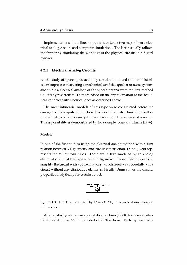
4 Acoustic Synthesis 99
Implementations of the linear models have taken two major forms: elec-
trical analog circuits and computer simulations. The latter usually follows
the former by simulating the workings of the physical circuits in a digital
manner.
4.2.1 Electrical Analog Circuits
As the study of speech production by simulation moved from the histori-
cal attempts at constructing a mechanical artificial speaker to more system-
atic studies, electrical analogs of the speech organs were the first method
utilised by researchers. They are based on the approximation of the acous-
tical variables with electrical ones as described above.
The most influential models of this type were constructed before the
emergence of computer simulation. Even so, the construction of real rather
than simulated circuits may yet provide an alternative avenue of research.
This is possibility is demonstrated by for example Jones and Harris (1996).
Models
In one of the first studies using the electrical analog method with a firm
relation between VT geometry and circuit construction, Dunn (1950) rep-
resents the VT by four tubes. These are in turn modeled by an analog
electrical circuit of the type shown in figure 4.3. Dunn then proceeds to
simplify the circuit with approximations, which result - purposefully - in a
circuit without any dissipative elements. Finally, Dunn solves the circuits
properties analytically for certain vowels.
Figure 4.3: The T-section used by Dunn (1950) to represent one acoustic
tube section.
After analysing some vowels analytically Dunn (1950) describes an elec-
trical model of the VT. It consisted of 25 T-sections. Each represented a

4 Acoustic Synthesis 100
tube with a length of 0.5 cm and a cross-sectional area of 6 cm2. This sys-
tem could be divided into two cavities by adding a constriction impedance
shown in figure 4.4 labeled as “tongue”. It could be added between any
two of the T-sections. When excited with a suitable signal, this system pro-
duced good enough vowels to be found useful in research
Figure 4.4: The electrical circuit used by Dunn (1950) to simulate the VT.
Stevens, Kasowski, and Fant (1953) built an electrical model of the VT
with 35 tube sections represented by π-sections of the type shown in figure
4.5. Each of these had a virtual length of 0.5 cm and an individually variable
area and damping. The model’s length could adjusted in 0.5 cm increments
by setting the impedance, which represented the lips, after any of the π-
sections. Finally, the model could be excited either from the glottal end or
by adding a noise source between any two of the π-sections.
Figure 4.5: The π-section used by Stevens et al. (1953) to represent one
acoustic tube section. The impedances are explained in the text.
The sounds produced by the model were reported to differ from those
of real speech especially at high frequencies. While the model was quite
flexible in being able to produce also other sounds besides vowels, it was
limited to producing only sounds where the VT does not divide into more
then one tube.
4.2.2 Computer Simulation
Computer simulation of linear speech signal generation has followed the
path started by electrical analog circuit models. The most notable model

4 Acoustic Synthesis 101
by far is the Kelly-Lochbaum model, which has been expanded to two and
three dimensional versions in recent years. However, some studies have
employed other methods for moving the electrical analog circuits into dig-
ital simulations.
Models
The basic building block of the model developed by Kelly and Lochbaum
(1962) is shown in figure 4.6. The model’s principle is to model each tube
junction by the reflection and transmission coefficients derived in section
4.1.3. These are used both for a wave propagating towards the mouth and a
wave propagating towards the glottis. Time discretisation is accomplished
by adding a unit time delay in both directions or alternatively a double
delay in one direction only. These have the same overall effect, but the
latter version is computationally simpler.
Figure 4.6: The model of an acoustic tube junction by Kelly and Lochbaum
(1962) (picture from Mullen et al. (2006)). The blocks labeled z−1 represent
unit time delays. r stands for the reflection coefficient R and p± for sound
pressure waves. The last term is a function of both node and iteration step.
The original model was found to have a fairly bad voice quality, but sur-
prisingly good consonants. In conclusion, Kelly and Lochbaum (1962) state
that contemporary formant synthesis was more satisfactory. Nevertheless,
as is evident from later studies of articulatory speech synthesis, this is a
very successful model.
Badin and Fant (1984) propose a simulated electrical circuit analog
shown in figure 4.7. They also report some preliminary results from using
the model without the subglottal system. The model itself consists of tube
and horn section modeled with T-sections. Also, it has sources at the glottis
and possible constrictions.

4 Acoustic Synthesis 102
Figure 4.7: The circuit proposed by Badin and Fant (1984) to be used in
a computer simulation of the VT. The blocks labeled T[N,C+1,etc] are T-
sections, which represent acoustical tube sections.
Badin and Fant (1984) had all three types of energy losses in their
model. Viscous and heat conduction losses were represented by resis-
tive impedances in series with the Z1 impedance of Dunn’s T-section. In
addition, wall losses were represented by adding a resistive element in
parallel with the Z2 element.
Mullen et al. (2006) expand the Kelly-Lochbaum model into a 2D model
by constructing a rectilinear mesh of junctions. In this system a signal is
able to propagate in four directions from each junction instead of just two.
Thus, the cross-sectional area of each tube section is represented by the
number of junctions, that the model has across the VT.
The sound pressure pJ at each junction J can be calculated by solving
the finite difference equation 4.14.
pJ(n) =2
N
N∑
i=1
pi(n − 1) − pJ(n − 2), (4.14)
where n is the iteration step and N the number of junctions. Further-
more, the walls, the lips and the glottis are simulated by adding appropri-
ate reflections at the boundary nodes pB of the form defined by equation
4.15.
pB = (1 + R)p+1,J (4.15)
Mullen et al. (2006) compared their 2D model with a traditional 1D Kelly-
Lochbaum model. A sample of the simulated vowel spectrums is shown in

4 Acoustic Synthesis 103
figure 4.8. They found that the 2D version was not conclusively better than
the 1D version, but the comparison indicated that the 2D version had the
capacity to produce more natural speech sounds.
Figure 4.8: Predicted formants of [u] along with simulated frequency re-
sponses of 1D and 2D waveguide models (Mullen et al., 2006).
A 3D version of this technique was employed by El Masri, Pelorson,
Saguet, and Badin (1996) to investigate higher resonance modes of the VT.
As expected they found transverse modes of resonance to appear around 5
kHz.
4.3 Non-linear Models
Even though speech sound production does have non-linear qualities, the
linear model is an excellent first approximation. Therefore, rather then de-
fine a completely non-linear model, the model discussed below adds a non-
linear component to linear models. This has the advantage of keeping the
model modular and thus easier to manage.
4.3.1 Noise Generation Modeled with Vorticity
Sinder (1999) developed speech production model by applying discretised
fluid dynamics to the problem of generating noise within constrictions in
the VT. The model is valid not only for noise associated with fricatives, but
for noise associated with other speech sounds as well.
The model is based on the theory of vorpal sound generation. The prin-
ciples of this theory are summarised by figure 4.9.
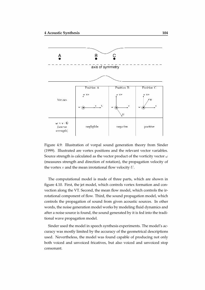
4 Acoustic Synthesis 104
Figure 4.9: Illustration of vorpal sound generation theory from Sinder
(1999). Illustrated are vortex positions and the relevant vector variables.
Source strength is calculated as the vector product of the vorticity vector ω
(measures strength and direction of rotation), the propagation velocity of
the vortex v and the mean irrotational flow velocity U .
The computational model is made of three parts, which are shown in
figure 4.10. First, the jet model, which controls vortex formation and con-
vection along the VT. Second, the mean flow model, which controls the ir-
rotational component of flow. Third, the sound propagation model, which
controls the propagation of sound from given acoustic sources. In other
words, the noise generation model works by modeling fluid dynamics and
after a noise source is found, the sound generated by it is fed into the tradi-
tional wave propagation model.
Sinder used the model in speech synthesis experiments. The model’s ac-
curacy was mostly limited by the accuracy of the geometrical descriptions
used. Nevertheless, the model was found capable of producing not only
both voiced and unvoiced fricatives, but also voiced and unvoiced stop
consonant.

4 Acoustic Synthesis 105
Figure 4.10: Relation ships of the submodels of the aerodynamic sound
generation model by Sinder (1999).
4.4 Summary
This chapter concludes the story of constructing an articulatory speech syn-
thesiser as far as it can be told within the limits of this thesis. All that
remains is to discuss the overall context and future of speech production
modeling. These are the topics of the final chapter.

5 Discussion 106
Chapter 5
Discussion
As this thesis draws towards its end, it is time to look back and share some
of my own thoughts on the discussions of the previous chapters.
5.1 Data Acquisition
While the current methods are very impressive, they are still - and probably
always will be - developing towards perfection. Based on the speed of
articulatory movements Perkell et al. (1992) sets the goal for the sampling
frequency band of articulatory measurements as 0 to 500 Hz.
To complement this I would set goals for spatial resolution and dimen-
sionality of the data: The former should be better than 1 mm, if possible by
at least one or two orders of magnitude just to be on the safe side. At the
same time the latter requirement should be set at full 3D acquisition with a
continuous sampling of space.
These requirements are quite hard to reach. However, different measure-
ment methods do already fulfil some of them: First, modern EMA systems
are capable of the kind of time resolution required by Perkell. Second, MRI
is already on the better side of a spatial resolution of 1 mm. This is en-
couraging even if MRI does not reach very good time resolution in full 3D
acquisitions. Third, ultrasound is also becoming what can be considered a
full 4D method.

5 Discussion 107
5.2 Models of Vocal Tract Geometry
In my opinion, it is clear, that 3D models of the VT are the only viable
choice in the long run. However, it is much harder to choose the methods
for parametrisation and generation of movement. For the parametrisation I
would consider two possibilities to be the best candidates: Statistical anal-
ysis in the near future and physiological modeling as time progresses.
As for the generation of movement, I do not think that I am really qual-
ified to answer. It is very hard to form an opinion based solely on the lit-
erature. For example, classical coarticulation studies disagree on the rela-
tion of vowel and consonant timing (see for example (Öhman, 1966), (Gay,
1977)). Even, if one would accept that the model should be a coarticulatory
one remains unclear as one has to consider the arguments put forward by
Xu and Liu (to be published).
5.3 Acoustic Synthesis
The basic model for modeling VT acoustics is well established as such.
What still remains unclear is the accuracy requirements, which should be
posed on different parts of the model. These requirements are not the same
for all sounds. Vowels require the general shape of the VT geometry to be
accurate, while in fricative production the main focus is on sudden changes
in the VT shape as air flows from the glottis to the mouth (Sinder, 1999).
To study the relative importance of an articulatory model’s components
they have to first be made as accurate as possible. Care has to be taken not
to emphasise any of the components over the others. Rather they have to
be made equally exact.
To this end, especially the glottal model and the radiation load connected
to the mouth have to be modeled carefully. Within the VT acoustic model-
ing needs to be expanded into the third dimension.
Also, new methods for acoustic modeling need to be considered. The
finite element method has been used recently to solve tube system reso-
nances (Peplow & Finnveden, 2004), (Lau & Tang, 2005). As our under-
standing of the mathematics involved in such models progresses, they will
most likely be found useful also in solving tube - or VT - dynamics.

5 Discussion 108
Another important consideration in acoustic synthesis has to be the de-
velopment of non-linear sound generation models. This may be even of
importance for vowel modeling as phonation is reported to give raise to
rotational flow within the VT, which in turn contributes to the resulting
sound (Barney et al., 1999), (Shadle et al., 1999).
5.4 Further Topics of Interest
Two topics have been only superficially present in this text: Glottal mod-
els and the performance evaluation of an articulatory speech synthesiser.
The former topic’s complexity is easily comparable to that of VT modeling.
Thus I can not present it here in any meaningful way. Instead, the latter
topic does allow a brief discussion.
5.4.1 Evaluating an Articulatory Speech Synthesiser
There are several ways an articulatory synthesiser may be evaluated. Some
of these have been given cursory attention in this text. Nevertheless, this
is a very important aspect of any synthesiser project. Therefore, to give
the reader some notion of the possibilities some common methods are pre-
sented below.
All speech synthesisers may be subjected to perceptual tests under dif-
ferent conditions. The tests most commonly try to establish a measure of
how natural and/or how intelligible the synthesiser is. In these tests the
results of synthetic speech are usually compared with the results of natu-
ral speech under the same test conditions. These conditions may include
noise and/or other distracting factors. Examples of the methodology can
be found in Möttönen (1999) and Ojala (2006).
An other evaluation method, common to all speech synthesisers, is di-
rect mathematical or statistical comparison of the produced speech with a
target sample of natural speech. With synthesisers, which are capable of ge-
ometric or visual output, an added dimension is comparison of articulatory
data with synthetic articulatory data, such as EPG (Engwall, 2001b). Most
statistical analysis methods employed in defining the model’s parameters
5 Discussion 109
already give one such measure - the amount of explained variance (see sec-
tion 3.2.3, page 71).
5.5 Possible Future Directions
Listing all possible directions for future research is not possible and an at-
tempt would not even be very interesting. For this reason I will give here
only two suggestions removing idealisations and taking the physical sim-
ulations even further from their current position.
5.5.1 Removing Idealisations
As the computational power available for research purposes continues to
grow, some of the traditional simplifications could be removed. As an ex-
ample, the VT is not a straight tube. The curvature does not affect the reso-
nances under 4kHz by more than 2% - 8% (Sondhi, 1986). Nevertheless this
effect should, in my opinion, be taken into account when aiming for truly
accurate articulatory synthesis.
5.5.2 Physical Simulations
One vision for the future might be a model where perhaps the tissues and
air are separate, but the air within and without the VT is handled by one
fluid dynamic model. Sound in such a model would be observed by listen-
ing to the model in its own numerical far field. Specifically, there would be
no separation between the turbulence model and the acoustic model. Both
would handled by simulating computationally the dynamical behaviour of
the air in the system. Detailed tools for this kind of aerodynamical model-
ing do exist and could be applied to aeroacoustic research.

5 Discussion 110
5.6 Conclusion
Recent research has produced some exciting results. Some could be covered
by this thesis, while others could not. As an example of the latter group one
should mention a finite element model of vocal folds, which is caused to
vibrate by the subglottal pressure (Thomson, Mongeau, & Frankel, 2005).
As such realistic models are becoming a standard in the area, it can be said
with good confidence, that we live in truly interesting times.
Bibliography and References 111
Bibliography and References
Al-Bamerni, A., & Bladon, A. (1982). One-stage and two-stage temporal
patterns of velar coarticulation. Journal of the Acoustical Society of America,
72, S104.
Alwan, A., Narayanan, S., & Haker, K. (1997). Toward articultatory-
acoustic models for liquid approximants based on MRI and EPG data.
Part II. The rhotics. Journal of the Acoustical Society of America, 101(2),
1078–1089.
Badin, P., Bailly, G., Elisei, F., & Odisio, M. (2003, August). Virtual Talking
Heads and audiovisual articulatory synthesis. In Proceedings of The 15th
International Congress of Phonetic Sciences (ICPhS -03) (pp. 193–197). IPA.
Badin, P., Bailly, G., Raybaudi, M., & Segebarth, C. (1998). A three-
dimensional linear articulatory model based on mri data. Proceedings
of the Third ESCA/COCOSDA International Workshop on Speech Synthesis
(pp. 249 – 254).
Badin, P., Bailly, G., Raybaudi, M., & Segebarth, C. (2002). A three-
dimensional linear articulatory model based on mri data. Journal of Pho-
netics, 30, 533 – 553.
Badin, P., & Fant, G. (1984). Notes on vocal tract computation. STL-QPSR,
25(2–3), 53–108.
Baer, T., Gore, J. C., Boyce, S., & Nye, P. W. (1987). Application of MRI to
the Analysis of Speech Production. Magnetic Resonance Imaging, 5, 1 – 7.
Baer, T., Gore, J. C., Gracco, L. W., & Nye, P. W. (1991). Analysis of vocal
tract shape and dimensions using magnetic resonance imaging. Journal
of the Acoustical Society of America, 90(2), 799 – 828.

Bibliography and References 112
Bangayan, P., Alwan, A., & Narayanan, S. (1996). From MRI and Acoustic
Data to Articulatory Synthesis: a Case Study of the Lateral Approxi-
mants in American English. Proceedings of the 4th ICSLP (pp. 793 – 796).
Barney, A., Shadle, C. H., & Davies, P. O. A. L. (1999). Fluid flow in a
dynamic mechanical model of the vocal folds and tract. I. Measurements
and theory. Journal of the Acoustical Society of America, 105(1), 444 – 455.
Beautemps, D., Badin, P., & Bailly, G. (2001). Linear degrees of freedom in
speech production: Analysis of cineradio- and labio-films data for a ref-
erence subject, and articulatory-acoustic modeling. Journal of the Acous-
tical Society of America, 109(5), 2165 – 2180.
Bell-Berti, F., & Harris, K. S. (1982). Temporal patterns of coarticulation: Lip
rounding. Journal of the Acoustical Society of America, 71(2), 449 – 454.
Beskow, J., Engwall, O., & Granstrom, B. (2003). Resynthesis of Facial and
Intraoral Articulation from Simultaneous Measurements. In Proceedings
of The 15th International Congress of Phonetic Sciences (ICPhS -03).
Black, A., & Taylor, P. (1997). Festival speech synthesis system: system docu-
mentation (1.1.1) (Technical report). CSTR, University of Edinburgh.
Blackburn, C. S. (1996). Articulatory Methods for Speech Production and Recog-
nition. PhD thesis, Trinity College Cambridge & Cambridge University
Engineering Department.
Branderud, P. (1985). Movetrack - a movement tracking system. Proceedings
of the French-Swedish Symposium on Speech (pp. 113 – 122). Grenoble.
Browman, C. P., & Goldstein, L. (1992). Articulatory phonology: An
overview. Phonetica, 49, 155 – 180.
C-K., C., & Wang, W. S.-Y. (1978). Use of optical distance sensing to track
tongue motion. Journal of Speech and Hearing Research, 21, 482 – 496.
Cohen, M., Beskow, J., & Massaro, D. (1998). Recent developments in facial
animation: an inside view. Proceedings of AVSP98 (pp. 201 – 206).
Cohen, M. M., & Massaro, D. W. (1993). Modeling Coarticulation in Syn-
thetic Visual Speech. In N. M. Thalman, & D. Thalman (Eds.), Models and
Techniques in Computer Animation (pp. 139 – 156). Tokyo: Springer-Verlag.
Coker, C. H. (1976). A model for articulatory dynamics and control. Pro-
ceedings of the IEEE, 64(4), 452 – 460.

Bibliography and References 113
Dart, S. (1987). A bibliography of X-ray studies of speech. Working papers
in Phonetics, UCLA Phonetics Laboratory Group, 66, 1 – 97.
Deller, Jr., J. R., Hansen, J. H. L., & Proakis, J. G. (2000). Discrete-Time Pro-
cessing of Speech Signals. IEEE Press. Originally published by Macmillan
1993.
Demolin, D., George, M., Lecuit, V., Metens, T., Soquet, A., & Raeymaekers,
H. (1997). Coarticulation and articulatory compensations by dynamic
MRI. Proceedings of Eurospeech ’97 (pp. 43–46).
Demolin, D., Metens, T., & Soquet, A. (2000). Real time MRI and articu-
latory coordinations in vowels. Proceedings of the 5th Speech Production
Seminar: Models and Data (pp. 86 – 93). München, Germany.
Dunn, H. K. (1950). The Calculation of Vowel Resonances, and an Electrical
Vocal Tract. Journal of the Acoustical Society of America, 22, 740 – 753.
El Masri, S., Pelorson, X., Saguet, P., & Badin, P. (1996). Vocal tract acoustics
using the transmission line matrix (TLM) method. In Proceedings of the
4th International Conference on Spoken Language Processing (pp. 953 – 956).
Engwall, O. (1999a). Modeling of the vocal tract in three dimensions. In
Proceedings of 6th European Conference on Speech Communication and Tech-
nology (Eurospeech 1999) (pp. 113–116).
Engwall, O. (1999b). Vocal tract modeling in 3D. TMH-QPSR, (1-2/1999),
31–38.
Engwall, O. (2000a). A 3D tongue model based on MRI data. In Proceed-
ings of International Conference on Spoken Language Processing 2000 (ICSLP
2000) (pp. III: 901–904).
Engwall, O. (2000b). Are statical MRI data representative of dynamic
speech? Results from a comparative study using MRI, EMA and EPG. In
Proceedings of International Conference on Spoken Language Processing 2000
(ICSLP 2000) (pp. I: 17–20).
Engwall, O. (2000c). Dynamical aspects of coarticulation in Swedish frica-
tives - a combined EMA & EPG study. TMH-QPSR, (4/2000), 49–73.
Engwall, O. (2001a). Considerations in Intraoral Visual Speech Synthesis:
Data and Modeling. In Proceedings of 4th International Speech Motor Con-
ference (pp. 23–26).
Bibliography and References 114
Engwall, O. (2001b). Using Linguopalatal Contact Patterns to Tune a 3D
Tongue Model. In Proceedings of 7th European Conference on Speech Com-
munication and Technology (Eurospeech 2001) (pp. 1475–1478).
Engwall, O. (2002, September). A three-dimensional linear articulatory
model based on mri data. Proceedings of 7th International Conference on
Spoken Language Processing (ICSLP 2002, Interspeech 2002).
Engwall, O. (2003). A revisit to the Application of MRI to the Analysis of
Speech Production - Testing our assumptions. In Proceedings of the 6th Int
Seminar on Speech Production.
Engwall, O. (2004, October 4–8). From real-time MRI to 3D tongue move-
ments. In S. H. Kim, & D. H. Youn. (Eds.), ICSLP 2004, Vol. II (pp. 1109 –
1112). Jeju Island, Korea.
Engwall, O. (2006). Speech production: Models, Phonetic Processes and Tech-
niques, Chap. Assessing MRI measurements: Effects of sustenation, grav-
itation and coarticulation., pp. 301 – 314. New York: Psychology Press.
Engwall, O., & Badin, P. (1999). Collecting and analysing two- and three-
dimensional MRI data for Swedish. TMH-QPSR, (3-4/1999), 11–38.
Engwall, O., & Beskow, J. (2003a). Effects of corpus choice on statistical
articulatory modeling. In Proceedings of the 6th Int Seminar on Speech Pro-
duction.
Engwall, O., & Beskow, J. (2003b). Resynthesis of 3D tongue movements
from facial data. In Proceedings of 8th European Conference on Speech Com-
munication and Technology (Eurospeech 2003).
Engwall, O., Wik, P., Beskow, J., & Granström, B. (2004, October 4–8). De-
sign strategies for a virtual language tutor. In S. H. Kim, & D. H. Youn.
(Eds.), ICSLP 2004, Vol. III (pp. 1693 – 1696). Jeju Island, Korea.
Ericsdotter, C. (2005). Articulatory-Acoustic Relationships in Swedish Vowel
Sounds. PhD thesis, Stockholm University, Stockholm, Sweden.
Eysenck, M. W., & Keane, M. T. (2000). Cognitive Psychology, A Student’s
Handbook. Psychology Press, Taylor & Francis Group, 4th edition.
Fagyal, Z. (2001). Phonetics and speaking machines: On the mechanical
simulation of human speech in the 17th century. Historiographia Linguis-
tica, 28(3), 289–330.
Fant, G. (1970). Acoustic Theory of Speech Production. Mouton, The Hague.

Bibliography and References 115
Feldman, A. G. (1966). Functional tuning of the nervous system with con-
trol of movement or maintenance of a steady posture - II Controllable
parameters of the muscles. Biophysics, 11, 565 – 578.
Flanagan, J. L. (1965). Speech Analysis, Synthesis and Perception. Springer-
Verlag.
Fletcher, S. G., Dagenais, P. A., & Critz-Crosby, P. (1991). Teaching Vowels
to Profoundly Hearing-Impaired Speakers Using Glossometry. Journal of
Speech and Hearing Research, 34, 943 – 956.
Fuchs, S., & Perrier, P. (1999). An EMMA/EPG study of voicing contrast
correlates in German. Proceedings of the 15th ICPhS (pp. 1057–1060).
Fujimura, O. (1991). Recording and interpreting articulatory data - mi-
crobeam and other methods. Proceedings of the XIIth ICPhS, Vol. 3 (pp.
120–124).
Gauffin, J., & Sundberg, J. (1978). Pharyngeal Constrictions. Phonetica, 35,
157 – 168.
Gay, T. (1977). Articulatory movements in VCV sequences. Journal of the
Acoustical Society of America, 62(1), 183–193.
Greenwood, A. (1997, April). Articulatory speech synthesis using diphone
units. IEEE International Conference on Acoustics, Speech, and Signal Pro-
cessing (ICASSP-97) (pp. 1635–1638).
Greenwood, A., & Goodyear, C. (1994). Articulatory speech synthesis using
a parametric model and a polynomial mapping technique. International
Symposium on Speech, Image Processing and Neural Networks (ISSIPNN ’94)
(pp. 595–598).
Guenther, R. B., & Lee, J. W. (1996). Partial Differential Equations of Mathe-
matical Physics and Integral Equations. Dover Publications, Inc. New York.
Hardcastle, W., Gibbon, F., & Nicolaidis, K. (1991). EPG data reduction
methods and their implications for studies of lingual coarticulation. Jour-
nal of Phonetics, 19, 251–266.
Harshman, R., Ladefoged, P., & Goldstein, L. (1977). Factor analysis of
tongue shapes. Journal of the Acoustical Society of America, 62(3), 693 –
707.
Harsman, R. (1970). Foundations of the PARAFAC procedure: Models

Bibliography and References 116
and procedures for an ’explanatory’ multi-modal factor analysis. UCLA
Working Papers in Phonetics 16 , University Microfilms No. 10085.
Heinz, J. M., & Stevens, K. N. (1964). On the Derivation of Area Functions
and Acoustic Spectra from Cineradiographic Films of Speech. Journal of
the Acoustical Society of America, 36, 1037.
Hirayama, M., Vatikiotis-Bateson, E., & Kawato, M. (1993). Pysiologically
based speech synthesis using neural networks. IEICE Transactions on
Fundamentals of Communications, Electronics, Information and Systems, E76-
A(11), 1898 – 1910.
Hixon, T. J. (1971). An Electromagnetic Method for Transducing Jaw Move-
ments during Speech. Journal of the Acoustical Society of America, 49, 603
– 606.
Honda, K. (1996). Organization of tongue articulation for vowels. Journal
of Phonetics, 24, 39 – 52.
Honda, K., Kurita, T., Kakita, Y., & Maeda, S. (1995). Physiology of the lips
and modeling of lip gestures. Journal of Phonetics, 23, 243 – 254.
Hoole, P., Nguyen-Trong, N., & Hardcastle, W. (1993). A comparative in-
vestigation of coarticulation in fricatives: electropalatographic, electro-
magnetic and acoustic data. Language and Speech, 36, 235 – 260.
Hoole, P., Zierdt, A., & Geng, C. (2003, August). Beyond 2D in articulatory
data acquisition and analysis. The 15th International Congress of Phonetic
Sciences (pp. 265 – 268).
Houde, R. A. (1967). A study of tongue body motion during selected speech
sounds. PhD thesis, University of Michigan.
Jones, K., & Harris, J. (1996, June). The silicon vocal tract. IEEE International
Conference on Neural Networks (pp. 902–907). IEEE.
Kaburagi, T., & Honda, M. (1996). A model of articulator trajectory forma-
tion based on motor tasks of vocal-tract shapes. Journal of the Acoustical
Society of America, 99, 3154–3170.
Kahle et al. (1984). Taschenatlas der Anatomie. Thieme-Verlag.
Keller, E. (1987). Phonetic Approaches to Speech Production in Aphasia and
Related Disorders, Chap. Ultrasound measurements of tongue dorsum
movements in articulatory speech impairments, pp. 93–112. San Diego,
CA: College-Hill Press.

Bibliography and References 117
Keller, E., & Ostry, D. (1983). Computerized measurement of tongue dor-
sum movements with pulsed echo ultrasound. Journal of the Acoustical
Society of America, 73(4), 1309–1315.
Kelly, J., & Lochbaum, C. (1962). Speech synthesis. In Proceedings of the 4th
International Congress on Acoustics (pp. Paper G42: 1–4).
Kiritani, S., Itoh, K., & Fujimura, O. (1975). Tongue-pellet tracking by a
computer controlled X-ray microbeam system. Journal of the Acoustical
Society of America, 48(6), 1516–1520.
Kitamura, T., Fujita, S., Honda, K., & Nishimoto, H. (2004). An Experimen-
tal Method for Measuring Transfer Functions of Acoustic Tubes. Proceed-
ings of the 8th ICSLP.
Klatt, D. H. (1987). Review of text-to-speech conversion for English. Journal
of the Acoustical Society of America, 82(3), 737–793.
Ladefoged, P., Anthony, J., & Riley, C. (1971). Direct measurement of the
vocal tract. Working papers in Phonetics, UCLA Phonetics Laboratory Group,
19.
Ladefoged, P., Harshman, R., Goldstein, L., & Rice, L. (1978). Generating
vocal tract shapes from formant frequencies. Journal of the Acoustical So-
ciety of America, 64(4), 1027 – 1035.
Lance, D., & van der Giet, G. (1974, August). A Computer On-line Method
for Measuring Articulatory Movements. In G. Fant (Ed.), Speech Commu-
nication Seminar (pp. 73 – 77). Stockholm.
Lau, C. K., & Tang, S. K. (2005). Sound transmission across duct constric-
tions with and without tapered sections. Journal of the Acoustical Society
of America, 117(6), 3679 – 3685.
Le Goff, B. (1997). Automatic modeling of coarticulation in text-to-visual
speech synthesis. In Proceedings of Eurospeech -97.
Le Goff, B., & Benoît (1997). A French-Speaking Synthetic Head. Proceedings
of AVSP’97.
Lemmetty, S. (1999). Review of Speech Synthesis Technology. Master’s
thesis, Helsinki University of Technology.
Liljencrants, J. (1971). Fourier series description of the tongue profile. STL-
QPSR, 4, 9–18.
Bibliography and References 118
Lindblom, B., & Sundberg, J. (1971). Acoustical consequences of lip, tongue
and jaw movements. Journal of the Acoustical Society of America, 50, 1166
– 1179.
Lundberg, A., & Stone, M. (1999). Three-dimensional tongue surface re-
construction: Practical consideration for ultrasound data. Journal of the
Acoustical Society of America, 106, 2858–2867.
MacMillan, A. S., & Kelemen, G. (1952). Radiography of the Supraglottic
Speech Organs. A.M.A. Archives of Otolaryngology, 55, 681–682.
Maeda, S. (1979). An articulatory model of the tongue based on a statistical
analysis. Journal of the Acoustical Society of America, 65(S22).
Maeda, S. (1990). Compensatory articulation during speech: evidence from
the analysis and synthesis of vocal-tract shapes using an articulatory
model. In W. J. Hardcastle, & A. Marchal (Eds.), Speech Production and
Speech Modelling (pp. 131 – 149). Kluwer Academic, Dordrecht.
Maeda, S., & Toda, M. (2003, August). Mechanical properties of lip move-
ments: How to characterize different speaking styles? The 15th Interna-
tional Congress of Phonetic Sciences (ICPhS -03) (pp. 189–192). IPA.
Mathiak, K., Klose, U., Ackerman, H., Hertrich, I., Kincses, W.-E., & Grod,
W. (2000). Stroboscopic articulography using fast magnetic resonance
imaging. Proceedings of the 5th Speech Production Seminar: Models and Data
(pp. 97–100). München, Germany.
Mermelstein, P. (1973). Articulatory model for the study of speech produc-
tion. Journal of the Acoustical Society of America, 53(4), 1070 – 1082.
Minifie, F., Kelsey, C., & Zagzebski, J. (1971). Ultrasonic Scans of the Dorsal
Surface of the Tongue. Journal of the Acoustical Society of America, 49(6),
1857–1860.
Mixdorff, H. (2002). An Integrated Approach to Modelling German
Prosody.
Möttönen, R. (1999). Perception of Natural and Synthetic Audiovisual
Finnish Speech. Master’s thesis, University of Helsinki.
Mullen, J., Howard, D., & Murphy, D. (2004, October 5-8). Acoustical Sim-
ulations of the Human Vocal Tract Using the 1D and 2D Digital Waveg-
uide Software Model. Proc. of the 7th Int. Conference on Digital Audio Effects
(DAFx’04). Naples, Italy.

Bibliography and References 119
Mullen, J., Howard, D., & Murphy, D. (2006). Waveguide Physical Mod-
eling of Vocal Tract Acoustics: Flexible Formant Bandwith Control from
Increased Model Dimensionality. IEEE Transactions on Audio, Speech and
Language Processing, 14(3), 964 – 971.
Munhall, K., Vatikiotis-Bateson, E., & Tokhura, Y. (1995). X-ray Film
Database for Speech Research. Journal of the Acoustical Society of Amer-
ica, 98(2), 1222–1224.
Narayanan, S., Alwan, A., & Haker, K. (1995). An articulatory study of
fricative consonants using Magnetic Resonance Imaging. Journal of the
Acoustical Society of America, 98(3), 1325–1347.
Narayanan, S., Alwan, A., & Haker, K. (1997). Toward articulatory-acoustic
models for liquid approximants based on MRI and EPG data. Part I. The
Laterals. Journal of the Acoustical Society of America, 101(2), 1064–1077.
Narayanan, S., Nayak, K., Lee, S., Sethy, A., & Byrd, D. (2004). An approach
to real-time magnetic resonance imaging for speech prodcution. Journal
of the Acoustical Society of America, 115(4), 1771–1776.
Öhman, S. E. G. (1966). Coarticulation in VCV Utterances: Spectrographic
Measurements. Journal of the Acoustical Society of America, 39(1), 151–168.
Öhman, S. E. G. (1967). Numerical Model of Coarticulation. Journal of the
Acoustical Society of America, 41(2), 310 – 320.
Ojala, T. (2006). Auditory quality evaluation of present Finnish text-to-
speech systems. Master’s thesis, Helsinki University of Technology.
Olive, J. P., Greenwood, A., & Coleman, J. (1993). Acoustics of American
English Speech : a dynamic approach, Chap. 3, pp. 65 – 72. Springer-Verlag.
O’Shaughnessy, D. (1987). Speech Communication, Human and Machine.
Addison-Wesley.
Parthasarathy, S., Schroeter, J., Coker, C., & Sondhi, M. (1989). Articula-
tory analysis and synthesis of speech. Fourth IEEE Region 10 International
Conference (TENCON ’89) (pp. 760–764). IEEE.
Parush, A., Ostry, D., & Munhall, K. (1983). A kinematic study of lingual
coarticulation in VCV sequences. Journal of the Acoustical Society of Amer-
ica, 74(4), 1115–1125.
Payan, Y., & Perrier, P. (1997). Synthesis of V-V sequences with a 2D biome-

Bibliography and References 120
chanical tongue model controlled by the Equilibrium Point Hypothesis.
Speech Communication, 22, 185–205.
Peplow, A., & Finnveden, S. (2004). A super-spectral finete element method
for sound transmission in waveguides. Journal of the Acoustical Society of
America, 116(3), 1389 – 1400.
Perkell, J., Cohen, M., Svirsky, M., Matthies, M., Garabieta, I., & Jackson,
M. (1992). Electromagnetic midsagittal articulometer (EMMA) systems
for transducing speech articulatory movements. Journal of the Acoustical
Society of America, 92(6), 3078–3096.
Perkell, J. S. (1969). Physiology of Speech Production: Results and Implications
of a Quantitative Cineradiographic Study. PhD thesis, MIT.
Rossing, T. D., Moore, F. R., & Wheeler, P. A. (2002). The Science of Sound.
Addison Wesley, 3rd edition.
Rubin, P., Saltzman, E., Goldstein, L., McGowan, R., Tiede, M., & Browman,
C. (1996). CASY and extensions to the task-dynamic model. Proceedings
of the 1st ESCA Tutorial and Research Workshop on Speech Producing Model-
ing - 4th Speech Production Seminar (pp. 125 – 128).
Rubin, P. E., Baer, T., & Mermelstein, P. (1981). An articulatory synthesizer
for perceptual research. Journal of the Acoustical Society of America, 70(2),
321 – 328.
Schroeter, J., Larar, J., & Sondhi, M. (1987, April). Speech parameter esti-
mation using a vocal tract/Cord model. IEEE International Conference on
Acoustics, Speech, and Signal Processing (ICASSP ’87) (pp. 308–311).
Schroeter, J., Larar, J., & Sondhi, M. (1988). Multi-frame approach for
parameter estimation of a physiological model of speech production.
IEEE International Conference on Acoustics, Speech, and Signal Processing
(ICASSP -88) (pp. 83–86). IEEE.
Shadle, C. H., Barney, A., & Davies, P. O. A. L. (1999). Fluid flow in a
dynamic mechanical model of the vocal folds and tract. II. Implications
for speech production studies. Journal of the Acoustical Society of America,
105(1), 456 – 466.
Sinder, D. J. (1999). Speech Synthesis Using an Aeroacoustic Fricative Model.
PhD thesis, The State University of New Jersey.
Sondhi, M. M. (1986). Resonances of a bent vocal tract. Journal of the Acous-
tical Society of America, 79(4), 1113–1116.
Bibliography and References 121
Sonies, B., Shawker, T., Hall, T., Gerber, L., & Leighton, S. (1981). Ultrasonic
Visualization of Tongue Motion During Speech. Journal of the Acoustical
Society of America, 70(3), 683–686.
Stark, J., Ericsdotter, C., Branderud, P., Sundberg, J., Lundberg, H.-J., &
Lander, J. (1999). The apex model as a tool in the specification of speaker-
specific articulatory behavior. Proceedings of the XIVth ICPhS (pp. 2279 –
2282).
Stark, J., Lindblom, B., & Sundberg, J. (1996). APEX and articulatory syn-
thesis model for experimental and computational studies of speech pro-
duction. TMH-QPSR, 2, 45–48.
Stevens, K. N., & Hanson, H. M. (2003, August). Production of Consonants
with a Quasi-Articulatory Synthesizer. The 15th International Congress of
Phonetic Sciences (ICPhS -03) (pp. 199–202). IPA.
Stevens, K. N., & House, A. S. (1955). Development of a Quantitative De-
scription of Vowel Articulation. Journal of the Acoustical Society of America,
27, 484 – 493.
Stevens, K. N., Kasowski, S., & Fant, C. G. M. (1953). An Electrical Analog
of the Vocal Tract. Journal of the Acoustical Society of America, 25, 734 – 742.
Stewart, J. Q. (1922). An Electrical Analogue of the Vocal Organs. Nature,
110, 188 – 189.
Stone, M., Dick, D., Douglas, A., Davis, E., & Ozturk, C. (2000). Modelling
the internal tongue using principal strains. Proceedings of the 5th Speech
Production Seminar: Models and Data (pp. 133–136). München, Germany.
Stone, M., & Lundberg, A. (1996). Three-dimensional tongue surface
shapes of English consonants and vowels. Journal of the Acoustical So-
ciety of America, 99(6), 3728 – 3737.
Sundberg, J., Johansson, C., Wilbrand, H., & Ytterbergh, C. (1987). From
sagittal distance to area: A study of transverse, vocal tract cross-sectional
area. Phonetica, 44(2), 76 – 90.
Teager, H. M. (1980). Some Observations on Oral Air Flow During Phona-
tion. IEEE Transactions on Acoustics, Speech and Signal Processing, ASSP-
28(5), 599–601.
Thomson, S. L., Mongeau, L., & Frankel, S. H. (2005). Aerodynamic transfer
of energy to the vocal folds. Journal of the Acoustical Society of America,
118(3), 1689 – 1700.
Bibliography and References 122
Tom, K., Titze, I., Hoffman, E., & Story, B. (1999). 3-D Vocal Tract Imaging
and Formant Structure: Varying Vocal Register, Pitch and Loudness. Sta-
tus and Progress Report, National Centre for Voice and Speech, University of
Iowa, 14, 101–113.
Tom, K., Titze, I. R., Hoffman, E. A., & Story, B. H. (2001). Three-
dimensional vocal tract imagin and formant structure: Varying vocal
register, pitch, and loudness. Journal of the Acoustical Society of America,
109(2), 742 – 747.
Uosukainen, S. (2006). Akustinen kenttäteoria. Lecture notes published by
Edita, Otaniemi.
Wrench, A., & Hardcastle, W. (2000). A multichannel articulatory speech
database and its application for automatic speech recognition. Proceed-
ings of the 5th Speech Production Seminar: Models and Data (pp. 305 – 308).
München, Germany.
Wrench, A., McIntosh, A., & Hardcastle, W. (1996). Optopalatograph
(OPG): A new apparatus for speech production analysis. Proceedings of
the 4th ICSLP (pp. 1589–1592).
Wrench, A., McIntosh, A., & Hardcastle, W. (1997). Optopalatograph: de-
velopment of a device for measuring tongue movement in 3D. Proceed-
ings of Eurospeech ’97 (pp. 1055–1058).
Wrench, A., McIntosh, A., Watson, C., & Hardcastle, W. (1998). Optopalato-
graph: real-time feedback of tongue movement in 3D. Proceedings of the
5th ICSLP (pp. 305 – 308).
Xu, Y., & Liu, F. (to be published). Tonal alignment, syllable structure and
coarticulation: Toward an integrated model.
Zheng, Y., & Hasegawa-Johnson, M. (2003). Analysis of the three-
dimensional tongue shape using a three-index factor analysis model.
Journal of the Acoustical Society of America, 113(1), 478 – 486.
Zierdt, A., Hoole, P., Honda, M., Kaburagi, T., & Tillman, H. (2000). Extract-
ing tongues from moving heads. Proceedings of the 5th Speech Production
Seminar: Models and Data (pp. 313–316). München, Germany.

A Webster’s Horn Equation 123
Appendix A
Webster’s Horn Equation
To describe wave propagation within the VT mathematically, we will use
the definitions given in table A.1.
Table A.1: Definitions for analysis of wave propagation in the VT
ρ density of the medium
ρ0 constant component of the density of the medium
p perturbation pressure (sound pressure)
q′ mass source
u particle velocity
U volume velocity
We will begin by supposing that the air within the VT is ideal gas. There-
fore we have the law of mass preservation and Euler’s equation:
∂ρ
∂t+ ∇ · ρu = ρq′ (A.1)
ρ0∂u
∂t+ ∇p = 0 (A.2)
As we take into consideration the absence of mass sources in the VT (q′ =
0) and the fact that the frequency range of interest (roughly from 100 to
3000 Hz) is fairly low in comparison with the frequencies of cross-mode
resonances (lowest effect is around 5 kHz for an average male VT), we can
consider the VT as an effectively one dimensional tube and thus get:
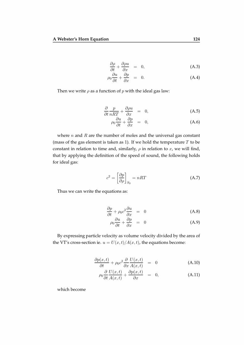
A Webster’s Horn Equation 124
∂ρ
∂t+
∂ρu
∂x= 0, (A.3)
ρ0∂u
∂t+
∂p
∂x= 0. (A.4)
Then we write ρ as a function of p with the ideal gas law:
∂
∂t
p
nRT+
∂ρu
∂x= 0, (A.5)
ρ0∂u
∂t+
∂p
∂x= 0, (A.6)
where n and R are the number of moles and the universal gas constant
(mass of the gas element is taken as 1). If we hold the temperature T to be
constant in relation to time and, similarly, ρ in relation to x, we will find,
that by applying the definition of the speed of sound, the following holds
for ideal gas:
c2 =
[∂p
∂ρ
]
S0
= nRT (A.7)
Thus we can write the equations as:
∂p
∂t+ ρ0c
2 ∂u
∂x= 0 (A.8)
ρ0∂u
∂t+
∂p
∂x= 0 (A.9)
By expressing particle velocity as volume velocity divided by the area of
the VT’s cross-section ie. u = U(x, t)/A(x, t), the equations become:
∂p(x, t)
∂t+ ρ0c
2 ∂
∂x
U(x, t)
A(x, t)= 0 (A.10)
ρ0∂
∂t
U(x, t)
A(x, t)+
∂p(x, t)
∂x= 0, (A.11)
which become
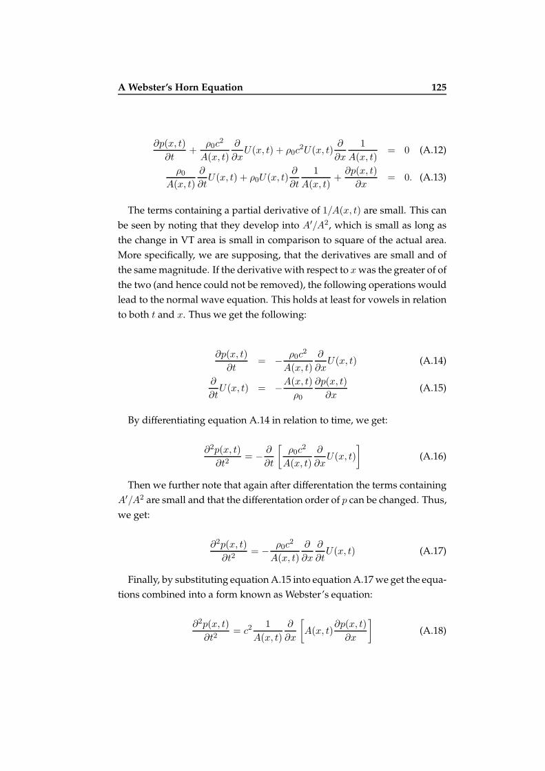
A Webster’s Horn Equation 125
∂p(x, t)
∂t+
ρ0c2
A(x, t)
∂
∂xU(x, t) + ρ0c
2U(x, t)∂
∂x
1
A(x, t)= 0 (A.12)
ρ0
A(x, t)
∂
∂tU(x, t) + ρ0U(x, t)
∂
∂t
1
A(x, t)+
∂p(x, t)
∂x= 0. (A.13)
The terms containing a partial derivative of 1/A(x, t) are small. This can
be seen by noting that they develop into A′/A2, which is small as long as
the change in VT area is small in comparison to square of the actual area.
More specifically, we are supposing, that the derivatives are small and of
the same magnitude. If the derivative with respect to x was the greater of of
the two (and hence could not be removed), the following operations would
lead to the normal wave equation. This holds at least for vowels in relation
to both t and x. Thus we get the following:
∂p(x, t)
∂t= −
ρ0c2
A(x, t)
∂
∂xU(x, t) (A.14)
∂
∂tU(x, t) = −
A(x, t)
ρ0
∂p(x, t)
∂x(A.15)
By differentiating equation A.14 in relation to time, we get:
∂2p(x, t)
∂t2= −
∂
∂t
[ρ0c
2
A(x, t)
∂
∂xU(x, t)
]
(A.16)
Then we further note that again after differentation the terms containing
A′/A2 are small and that the differentation order of p can be changed. Thus,
we get:
∂2p(x, t)
∂t2= −
ρ0c2
A(x, t)
∂
∂x
∂
∂tU(x, t) (A.17)
Finally, by substituting equation A.15 into equation A.17 we get the equa-
tions combined into a form known as Webster’s equation:
∂2p(x, t)
∂t2= c2 1
A(x, t)
∂
∂x
[
A(x, t)∂p(x, t)
∂x
]
(A.18)

A Webster’s Horn Equation 126
A.1 Notes on Deriving the Equation
The idealisations involved in deriving equation A.18 have certain conse-
quences some of which I will discuss here.
First and foremost is the step where we remove two of the original three
spacial dimensions. As a result, there can be no cross-modes or vortices
present in the resulting model. The absence of cross-modes should not be a
problem as long as we are not interested in formants beyond the first two,
but after that the effects are probably considerable. Likewise, the absence
of vortices or turbulent flow does not cause problems, if we are interested
in modeling only vowel production. However, consonant - and escpecially
fricative, modeling will need some other mechanism for producing turbu-
lent noise, if the above 1D equations A.8 and A.9 are used.
A further thing to consider are the assumptions, which removed losses
from the model. These are, firstly, the fact, that we implicitly assume the
walls of the vocal tract to be infinitely hard. Thus no energy is dissipated
as sound propagation into the tissues surrounding the VT. Secondly, we
assumed the air within the VT to be ideal gas. This in turn means, that
there are no viscous or heat conduction losses within the gas itself. Fortu-
nately, these types of losses can be, and successfully have been, added to
1D models.
Finally, we should remember, that the equations A.1 and A.2 assume that
there is no flow within the VT, and the assumption, that A′/A2 is small. The
first of these clearly does not hold. The flow can of course be assumed to
behave in a suitably regular way so, that its effects can be left out as a minor
approximation. Nevertheless, as models of speech production grow more
sophisticated this idealisation has to be eventually removed. As for the
second assumption, it holds - as stated above - only for vowels. Especially
in the case of plosive or tremulant sounds, such an approximation can not
be said to be true.