a research agenda for measuring gdp at the county level wp_research agenda... · a research agenda...

A Research Agenda for Measuring GDP at the County Level

Ledia Guci, Charles Ian Mead, Sharon D. Panek

Bureau of Economic Analysis

July 2016

Abstract

The Bureau of Economic Analysis (BEA) publishes gross domestic product (GDP) statistics for the nation,

states, and metropolitan areas. GDP by county statistics would provide a much richer picture of the

geographic distribution of the nation’s economic activity to assist analysts in the assessment of local

economic performance and policymakers in the development of strategies to promote economic

growth. This paper identifies a research agenda to produce such statistics and uses a simple

methodology to produce county GDP statistics for a few case studies based on county earnings by

industry. These experimental statistics illustrate the kind of information on industry structure and local

economic activity that can be uncovered with GDP by county statistics. Further research is needed to

identify additional source data and investigate alternative methodologies and various modelling

techniques that can be used to generate proper output measures at the county level.

The authors thank Jacob Hinson, Frank Baumgardner, and Jonas Wilson for research assistance and support and Joel Platt for valuable comments and guidance.

2

Ten years ago, the Bureau of Economic Analysis (BEA) released for the first time gross domestic

product (GDP) by metropolitan area statistics. At the time, these statistics represented a further step in

meeting BEA’s long‐standing goal of providing more detail in depicting the geographic distribution of the

nation’s economic activity to assist analysts in the assessment of local economic performance and

policymakers in the development of strategies to promote economic growth. The next step in this

direction will be the development of GDP by county statistics to support economic planning at finer and

alternative levels of geographic detail.

This paper discusses the need for GDP by county statistics and identifies a research agenda to

produce such statistics. The agenda builds upon the methodology used to create GDP by metropolitan

area statistics and identifies industries where additional work is needed to ensure that BEA’s high data

quality standards are met. In addition, new data sources are identified that could be used in producing

county‐level statistics that may also improve other BEA regional GDP statistics. Further work needed to

determine the level of industry detail that could be provided in county‐level statistics, while protecting

confidential company information, is also discussed. Finally, a few experimental results are presented.

Motivation

The most recent U.S. recession and recovery have highlighted the need for more geographically detailed

regional economic statistics. BEA’s currently available regional GDP and income statistics provide insight

into different economic experiences across broad economic regions. However, often the level of

geographic detail they provide is insufficient for policy makers and regional planners to direct resources

to the specific locations that would benefit most. In many cases, counties that are in most need of

economic development assistance are not part of a metropolitan area and are only captured in much

broader regional aggregates, such as GDP by state. Even within metropolitan areas, more detailed

county‐level GDP statistics would greatly benefit resource allocation decisions.

3

The addition of GDP by county statistics would potentially provide at least three benefits. First,

the new statistics would help paint a much richer and more detailed picture of geographic distribution

of U.S. economic activity. Second, the new statistics would allow for more detailed analyses to support

resource allocation decisions and better predict the long‐term impacts of different developmental

strategies. Third, the process of developing the new statistics would likely lead to improvements in

related GDP by state and metropolitan area statistics.

Rich picture of national trends. A practical advantage of GDP by county statistics is that the

measures for individual counties can be summed to provide measures of activity that closely

circumscribes a related economy irrespective of state or metropolitan area lines. One notable bright

spot during the latest U.S. recession and recovery was the natural resource boom in the areas where the

Bakken and Marcellus Shale Formations are located. Because mining and extraction occurs where

natural resources are found, this activity often occurs in rural areas that are not clearly circumscribed by

state or metropolitan area boundaries.

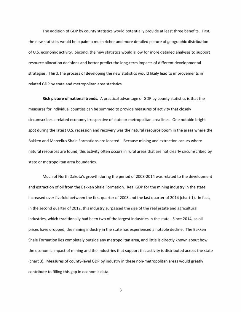
Much of North Dakota’s growth during the period of 2008‐2014 was related to the development

and extraction of oil from the Bakken Shale Formation. Real GDP for the mining industry in the state

increased over fivefold between the first quarter of 2008 and the last quarter of 2014 (chart 1). In fact,

in the second quarter of 2012, this industry surpassed the size of the real estate and agricultural

industries, which traditionally had been two of the largest industries in the state. Since 2014, as oil

prices have dropped, the mining industry in the state has experienced a notable decline. The Bakken

Shale Formation lies completely outside any metropolitan area, and little is directly known about how

the economic impact of mining and the industries that support this activity is distributed across the state

(chart 3). Measures of county‐level GDP by industry in these non‐metropolitan areas would greatly

contribute to filling this gap in economic data.

4

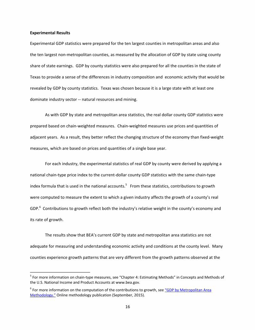
In the region circumscribed by the Marcellus Shale Formation, much of the economic growth

during the 2013‐2014 period was supported by mining activities related to the development and

extraction of natural gas. The Marcellus Shale Formation crosses many states including large portions of

West Virginia and Pennsylvania (chart 4). In West Virginia, real GDP for the mining industry more than

doubled during this period (chart 2) and in the second quarter of 2014 became the state’s largest

industry.

In the case of the Marcellus and Bakken Shale Formations, county‐level statistics for the mining

industry would allow data users to customize areas that include portions of metropolitan areas and non‐

metropolitan areas and cross state boundaries to measure the impact of mining activities on economic

growth in these specifically designed areas. The same type of analysis could be performed to measure

the impact of development of other types of natural resources. Such information would prove

invaluable in determining energy policy and anticipating the effects that the development of alternative

resources may have across communities in the nation.

Another industry that played a prominent role in the recent recession and recovery is housing

services, which is highly localized in nature. The effects of the recent housing boom and bust in many

parts of the nation are well measured and easily identifiable in the GDP statistics for Arizona, Florida,

and Nevada. Even the effects in particular metropolitan areas can be seen in the GDP by metropolitan

statistics. California serves as an interesting example: The industrial structure of the state closely

mirrors that of the U.S. economy, yet one can see how the housing bust in the Los Angeles, San

Francisco, and El Centro metropolitan areas contributed to a slightly longer and deeper recession for the

state compared to the nation.

Despite our knowledge of housing market activity in state and metropolitan areas, little is

known about some of the systematic variation in the value of housing services outside of metropolitan

5

areas. The economy of Teton County, Wyoming, is currently dominated by a growing recreation and

tourism industry spurred by wealthy travelers and second home buyers, yet Teton County is not large

enough to be designated a metropolitan area, and no official measures related to the contribution of

housing services to the local economy exist.

The recent experiences of Lincoln County, Montana, are much different than those in Teton

County. Lincoln County is characterized by an aging population and high levels of economic hardship.

This hardship is often attributed to the loss of mining and timber jobs and the out‐migration of the

younger working population. Again, this county is not large enough to constitute its own metropolitan

area.

The dramatic differences between Teton County and Lincoln County can be seen by comparing

local sources of personal income. In Teton County, the largest source of personal income is interest,

dividends, and rental income (table 1). In 2014, per capita income from these sources was $143,683.

Per capita income from earnings in Teton County in the same year was only $45,983. In Lincoln County,

per capita income from social assistance was $11,263. Per capita income from earnings was only slightly

larger at $12,915. Per capita income from interest, dividends, and rents stood at only $6,818.

Even though much can be said about the differences in the sources of income across counties,

no official statistics on the value of goods and services produced within counties exist, including housing

services, that can be used to compare production activities associated with different types of economies

at the county level.

The changing landscape of housing services across the U.S. economy is likely to become an

increasingly important topic of interest to many economists as baby boomers continue to buy second

homes or retire later in their lives. Having county‐level information to identify trends in the value of

housing services and investigate their relation to the industries that typically develop to support an

6

aging population will be an invaluable asset for a better understanding of local economic developments

for years to come.

Better resource allocation. For local officials and regional planners tasked with addressing the

development needs of areas falling outside metropolitan areas, the availability of reliable and consistent

statistics for analyzing the potential economic impact of alternative development options is very limited.

While BEA’s local area personal income (LAPI) statistics provide insight into county‐level economic

conditions, they do not provide a complete picture of the local economy. LAPI statistics provide

important information regarding the sources of income received by local residents and the amounts

earned by industry within a county, but do not measure the value of goods and services produced in a

county.1 This can leave a very incomplete and inaccurate picture of economic activity in counties with

economies dominated by capital‐intensive industries.

While the LAPI statistics provide good indicators of areas where the need for social assistance is

greatest, they are not sufficient for analyzing the efficacy of larger strategies for determining the types

of industries that should be supported to spur local business development. A consistent set of GDP by

county statistics would complement BEA’s LAPI estimates and support the analysis of broader economic

development strategies in at least three ways. First, these statistics would provide a more accurate and

comprehensive depiction of the industrial make up and condition of the local economy and assist in

developing policies and targeted incentives that would be most effective in promoting economic

growth. Second, these statistics could be used in developing promotional materials to attract further

business activity to a local area. Third, officials and planners in multi‐county metropolitan areas would

have more complete information for identifying the strengths and weaknesses of their local economy

and targeting their economic development efforts in counties with the greatest need.

1 Earnings is the sum of three components of personal income—wages and salaries, supplements to wages and salaries, and proprietors' income.

7

Long‐term strategies. The development of a time series of GDP by county statistics would not

only assist in identifying the current economic conditions in local economies, but it would also support

research related to understanding local economic dynamics and the longer‐term impacts of different

development strategies. In particular, with a time series of historic GDP by county data, research could

be conducted to see how different developmental strategies affect the long‐term trajectory of an

economy and how they are related to long‐term trends in local demographics. In addition, trends in

GDP by county data could be used to evaluate the effectiveness of incentive programs used to support

development strategies. Previously, only employment data were available to evaluate the benefit of

bringing additional businesses to the local economy, which does not provide a complete picture of the

expansion.

The provision of GDP by county statistics could fill in the gap by allowing for examinations of the

specific industries that typically grow to support aging populations—for example, local economic

developers could better understand how the local industrial structure typically changes over time in

response to an aging population. Local developers could also better understand how supporting the

growth in a particular set of industries may attract more skilled workers to their community. Further,

examinations could be performed to determine whether attracting new business increases the total

income received within a specific county or a nearby metropolitan area over the long run.

Other improvements. The development of GDP by county statistics will potentially provide

ancillary benefits that lead to improvements in the accuracy and reliability of GDP by metropolitan area

statistics. Currently, GDP for a metropolitan area is calculated by using earnings statistics to

geographically distribute state GDP to metropolitan areas.2 For many industries, more detailed

2The metropolitan (statistical) areas definitions used for BEA statistics are defined by the U.S. Office of Management and Budget (OMB). These definitions identify standardized county‐based areas having at least one urbanized area with a population of 50,000 or more plus adjacent territory that has a high degree of social and

8

methodologies and source data will need to be developed and identified to produce and publish county‐

level statistics that meet BEA’s high quality standards. The development of new methodologies and

identification of new data sources needed for the estimates of GDP for these more challenging

industries will likely lead to improvements in BEA’s GDP by state and metropolitan area statistics.

Methodological Considerations

GDP by county is a measure of the value of production that occurs within the geographic boundaries of

a county. It can be computed as the sum of the value added originating from each of the industries in a

county. An industry’s value added is defined as the difference between its gross output (sales and other

operating income, commodity taxes, and inventory change) and its intermediate inputs (purchases of

goods and services from other industries in the U.S. or imported that are used in production).

While value added by industry for BEA’s GDP by state statistics is derived from various data

sources at the state level, a simple method for deriving experimental county‐level GDP statistics is to

geographically allocate state GDP to counties using county earnings data. For many industries, earnings

are considered to be reasonable indicators of economic activity across geographic areas because overall

they represent more than 60 percent of GDP by industry.

County earnings statistics are available from BEA’s LAPI statistics. 3 Earnings consist of wage and

salary disbursements, supplements to wages and salaries, and proprietors’ income. These statistics are

based on data in large measure from the Quarterly Census of Employment and Wages (QCEW) series

from the Bureau of Labor Statistics. Statistics for the most recent year covered in a GDP by county

release would rely directly on the QCEW because county earnings would not be available at the time of

economic integration with the core as measured by commuting ties. The most recent definitions of these areas that are currently used by BEA are provided in OMB Bulletin No. 13‐01. 3 For a discussion of the methodology used to compute local area personal income see “Local Area Personal Income

and Employment.” Online methodology publication (May 2014).

9

publication. The same methodology is used for the most recent year covered in a GDP by metropolitan

area release.

Drawing from the methodology of the GDP by metropolitan area, the methodology used for this

paper to get a first look at GDP by county estimates for a few case studies involves two steps.4 In the

first step, for each industry , initial GDP by county statistics are computed by allocating state GDP to

the corresponding counties using the industry county‐to‐state earnings shares:

, ,, ,

, ,, ,

This allocation ensures that the county‐level statistics are consistent with the metropolitan area and

state counterparts. In the second step, the statistics are carefully evaluated and reviewed to ensure the

experimental county GDP statistics are sensible and consistent with other statistics in the regional

economic accounts.

The allocation approach serves only as a starting point to assist in scoping out a reaseach

agenda for developing GDP by county statistics. Further research is required in at least three areas:

discovery of additional source data, investigation of alternative methodologies, and investigation of

various modelling techniques that can be used to generate proper output measures at the county level.

The approach used in this paper relies on the premise that the distribution of earnings by

industry across all counties in a state provides a sensible approximation to the distribution of the output

by industry across all counties. Specifically, using earnings to allocate the state output to counties

assumes that the factors of production such as capital‐labor ratios required to produce the output of

each industry are similar between the county and the state where the county resides. Furthermore, it

4 For a discussion of the methodology used to compute gross domestic product by metropolitan area, see “GDP by Metropolitan Area Methodology.” Online methodology publication (September, 2015).

10

assumes that the state‐level industry earnings‐to‐output relationships hold at the county level so that

the variation in GDP across areas is primarily determined by the variation in earnings.

A major advantage of the approach used in this paper is that it is simple, transparent, and

should generally perform well since these relationships tend to hold reasonably well for many

industries. The simplicity of the approach allows for research efforts to focus on identifying additional

source data and developing new methodologies for the industries that are more difficult to measure

through earnings. Incorporating additional source data may also improve the statistics for industries

where the location of earnings tends to differ from the location of production.

Capital‐intensive industries can be underestimated by earnings because corporate income is not

reflected in earnings. Capital‐intensive industries are industries whose production relies heavily on

physical or financial capital. The former are often found in industries that utilize heavy equipment while

the latter characterizes financial services industries. The measurement of the economic activity for

these industries may be improved with the development of hybrid methodologies that supplement

earnings data with additional information that includes business source data.

One way to identify industries that are capital intensive is to compute the ratio of earnings to

GDP. A small value of the earnings‐to‐GDP ratio suggests that the industry is capital intensive. Table 2

shows 2013 earnings‐to‐GDP ratios for 19 aggregated industry sectors at the national level. Mining,

utilities, and real estate, and rental, and leasing are industry sectors that are relatively more capital

intensive. For these industry sectors, additional source data have been identified that may improve

their measures of output. These data along with additional data identified for some of the industries

under the sectors of finance and insurance and transportation and warehousing are described in the

next section.

11

Additional Source Data

As part of researching the feasibility of producing GDP statistics for counties, BEA has identified

additional source data for the real estate, mining, utilities, banking, and air transportation industries

that may be used to supplement earnings to generate the respective county GDP statistics. Source data

for these industries are consistently available to possibly improve the quality of the related measures.

Mining and real estate. Additional data for the mining and real estate industries would improve

statistics by accounting for the income earned from sole proprietorships and partnerships, which are

common in these two industries. This income, as tabulated by the Internal Revenue Service, is included

in the county where the owner or partner resides, which may differ from the county where the

economic activity took place. Both mining and real estate are capital intensive; therefore, the statistics

may also be improved by including data at the business level.

Limited data sources are available at the county level for mining businesses. The Department of

Energy provides maps and underlying value of production data for different types of mining as shown

for coal mining (chart 5). These data may be available to augment the earnings data to improve the

ability to assign a location to GDP produced for the mining industry at the county level.

Two data series published by the Census Bureau could be used along with earnings to improve

the real estate industry statistics. Median home values are published in the American Community

Survey and sales and revenues are published in the Economic Census.

Utilities. The Federal Energy Information Administration (EIA) publishes generating capacity by

plant. This information combined with financial data from the EIA has been used previously to improve

estimates of GDP by state, and could be used to distribute revenue data to the county level. EIA also

publishes revenue by state and by company, and lists the counties in which each company operates;

however, they do not publish revenue or operating data at the county level. Platts Energy Information is

12

a subscription‐based provider of utility data. Subscribers have access to detailed maps showing power

plants and their characteristics and a database similar to one published by EIA. Platts Energy

Information, however, includes county‐level data.

Banking. The Federal Deposit Insurance Corporation’s Summary of Deposits publishes bank

deposits by branch for every active bank. These data can be used to compute the shares of bank branch

deposits for each county. Deposit levels have proven to be an accurate indication of the location of GDP

produced by this industry at the state level and a reasonable indication of trends in the industry’s

growth.

Air transportation. Additional source data are important for the air transportation industry

when the trends in corporate income and earnings differ. In cases where the corporate income

component of GDP is positive while earnings are negative, additional data are needed to compute GDP.

Much of the source data used to compute state GDP statistics are available at the firm level and

can be used to develop a county data series. The two primary sources are financial data and passenger

data published by the Bureau of Transportation Statistics. Financial data are available for air carriers

with annual operating revenues over $20 million and flight data are available by carrier for both

passengers and freight. The flight data include: origin, destination, transported passengers, freight and

mail. Combining the firm‐level data with earnings statistics will help capture GDP produced in counties

with large transportation hubs as well as counties whose air transportation industry is smaller.

Corroborative Information

Once the GDP by county statistics are developed, BEA will evaluate the quality of the statistics using a

variety of independent data sources such as trade associations, company publications, and subscription

13

databases. The sources have been selected to identify the largest employers and trends in labor, to

characterize the local business climate, and to identify trends in selected industries.

Labor trends. Trends in earnings can be volatile at the county level and data corroboration will

help ensure the quality of GDP by county statistics. BEA has identified several sources of information on

local labor trends. LexisNexis and state departments of labor publish data on the largest employers and

their employment levels. These data can be used to analyze industry trends for local economies. In

addition, Worker Adjustment and Retraining Notification (WARN) reports, also from state governments,

show which industries experienced a decline in their workforce.

The National Establishment Time‐Series (NETS) database can be used to corroborate the

geographic assignment and trends in labor. The database offers a rich resource for labor, place of

operation, relocation data, and financial information for over 54 million establishments. Analysis of the

NETS data provides a context for trends in county GDP and will help identify outliers that require further

review.

Business climate. Data on economic development incentives and incentivized deals provide

critical information on new and expanded business. BEA has located data on state and local incentive

programs from government offices, Good Jobs First, C2er, and the New York Times database. In

addition, Conway Data publishes ICA incentives, which is a comprehensive database that includes new

investments, expansion investments, and relocation‐ or restructuring‐ related investments. To be

included, investment projects must create new employment while retaining existing employment and

meet a minimum level of capital investment. Nonfinancial incentives such as infrastructure

development are also included. Each source provides firm‐level data and includes the industry and the

value of the incentive, which suggests the size of the venture and will help analyze growth in local

economies.

14

Financial data for corporations can be used to assess whether earnings statistics captured the

trend and distribution of GDP. Financial statements from the Securities and Exchange Commission

database, the NETS database, and CompuStat provide information that can be used to corroborate GDP

statistics or to identify statistics that require further review.

Industry data. Independent data sources for the mining, real estate, and agriculture are very

important to the corroboration of GDP statistics. As mentioned previously, mining and real estate

industries are capital intensive and also tend to have owners who do not live near where production

occurs, which may skew the earnings data.

BEA can use rig counts and value of production in the mining industry from DrillEdge and Baker

Hughes to analyze the trend shown in GDP. This information can also be used to corroborate the

geographic assignment and relative production level of local areas for the industry.

GDP for the real estate industry will be compared to median home values from the National

Association of Realtors and housing starts by the Census Bureau. Building reports published by county

governments offer insight into the commercial real estate market for their local economy. While labor‐

intensive, the reports can be used to gather data on new commercial real estate development. Conway

Data’s New Plant Report is the most detailed database of commercial real estate development. The

database contains 178,000 new plant and expansion records going back to 1989.

The farming industry is one of the most challenging industries to measure partly due to the

effect weather has on the industry. The U.S. Department of Agriculture publishes data on crops by

county and their yields. This information will be used to investigate which crops are driving the local

agriculture industry. Information from Federal Emergency Management Agency on the timeline of

severe weather events and the magnitude of crop losses indicates which counties are affected and the

15

relative impact. Collectively, these sources will be used to analyze the statistics and refine the

methodology.

Corroboration is an important stage in the process of computing GDP by county statistics. It is

at this stage that BEA’s regional expertise is most essential to identify independent sources of

information and to evaluate the data collectively within the framework of regional economics.

Industry Detail

One aspect of the GDP by county statistics that needs further consideration is the level of industry detail

to be made available in the GDP by county statistics. First, consideration needs to be given to choosing

a level of industry detail that ensures protection of confidential information on companies. Second,

consideration should also be given to the quality of the source data to ensure that the GDP by county

statistics maintain high quality standards.

Most of the data sources that would be used to supplement and corroborate the GDP by county

statistics are not confidential. However, the earnings data, which would be a primary data source for

GDP by county statistics for most of the industries, rely on confidential wages and salaries data from the

Bureau of Labor Statistics and proprietors’ income data from the Internal Revenue Service. These

underlying source data need to be protected to avoid revealing any confidential information.

The county GDP statistics would likely be published at a higher level of industry aggregation than

the GDP by metropolitan area statistics. An initial assessment would be conducted at the level of the 19

aggregate industry sectors (table 2). If the results of the assessment prove unsatisfactory, aggregations

of multiple industry sectors would be considered.

16

Experimental Results

Experimental GDP statistics were prepared for the ten largest counties in metropolitan areas and also

the ten largest non‐metropolitan counties, as measured by the allocation of GDP by state using county

share of state earnings. GDP by county statistics were also prepared for all the counties in the state of

Texas to provide a sense of the differences in industry composition and economic activity that would be

revealed by GDP by county statistics. Texas was chosen because it is a large state with at least one

dominate industry sector ‐‐ natural resources and mining.

As with GDP by state and metropolitan area statistics, the real dollar county GDP statistics were

prepared based on chain‐weighted measures. Chain‐weighted measures use prices and quantities of

adjacent years. As a result, they better reflect the changing structure of the economy than fixed‐weight

measures, which are based on prices and quantities of a single base year.

For each industry, the experimental statistics of real GDP by county were derived by applying a

national chain‐type price index to the current‐dollar county GDP statistics with the same chain‐type

index formula that is used in the national accounts.5 From these statistics, contributions to growth

were computed to measure the extent to which a given industry affects the growth of a county’s real

GDP.6 Contributions to growth reflect both the industry’s relative weight in the county’s economy and

its rate of growth.

The results show that BEA’s current GDP by state and metropolitan area statistics are not

adequate for measuring and understanding economic activity and conditions at the county level. Many

counties experience growth patterns that are very different from the growth patterns observed at the

5 For more information on chain‐type measures, see “Chapter 4: Estimating Methods” in Concepts and Methods of the U.S. National Income and Product Accounts at www.bea.gov.

6 For more information on the computation of the contributions to growth, see “GDP by Metropolitan Area Methodology.” Online methodology publication (September, 2015).

17

state level; and even at the metropolitan area level. GDP by county statistics would provide important

information on industry composition and production activities that contribute to differences in

economic activity and growth among counties that are currently unavailable to policy makers, regional

planners and other users of regional economic data.

Top ten metropolitan and top ten non‐metropolitan area counties. Comparisons of the

contributions to county GDP growth from 2012 to 2013 for selected aggregated sectors across the two

sets of counties reveal several important differences in industry composition and growth (table 3 and

table 4).

Metropolitan area counties generally experienced relatively slower, but more uniform growth

across all industries compared with non‐metropolitan area counties. The range of growth in the

metropolitan area counties was 6.5 percent. In contrast, the range of growth in the non‐metropolitan

area counties was much wider ‐‐ 25.9 percent.

Examination of the industry‐level contributions to county growth for these areas shows that

growth in the metropolitan area counties was generally driven by the private service‐producing

industries. This contrasts with non‐metropolitan counties where growth was primarily driven by private

goods‐producing industries. These generalizations, however, do not apply in all cases.

Dallas County and Harris County in Texas, unlike other metropolitan counties, had sizable

contributions to growth from the natural resources and mining sector. Eddy County, New Mexico,

Williams County, North Dakota, and Merrimack County, New Hampshire, are exceptions among non‐

metropolitan counties, with significant contributions from private services‐producing industries. In fact,

Merrimack County exhibits industry contribution patterns that more closely resemble the larger

metropolitan area counties.

18

State of Texas. The experimental county statistics for the state of Texas provide rich detail on

the industry composition and the geographic distribution of the state’s economic activity. In addition,

they highlight the differences in the industrial structure and economic experiences of counties that are

currently masked in GDP by state and GDP by metropolitan area statistics.

Real GDP in Texas grew 5.5 percent from 2012 to 2013. Almost half the growth was attributable

to the manufacturing and the natural resources and mining sectors (table 5). The state’s growth rate

and industry composition to growth are dominated by its metropolitan areas, which accounted for over

90 percent of the state’s GDP in 2013. The non‐metropolitan portion of the state grew almost a full

percentage point slower than the metropolitan portion and exhibited higher industry contributions to

growth by the natural resources and mining sector and lower contributions to growth by the

manufacturing and the service‐producing sectors.

BEA’s current GDP by metropolitan area statistics capture the variation in growth and the

distribution of the state’s economic activities across metropolitan areas, but they do not capture the

rich variation in growth and distribution of these activities across counties within metropolitan areas.

For example, real GDP in the Dallas‐Fort Worth‐Arlington metropolitan area, one of the largest

metropolitan areas in Texas, grew 5.3 percent growth from 2012 to 2013 (table 6). The growth in this

metropolitan area, while similar in pace to the aggregate metropolitan portion of Texas, differed

significantly in terms of industry contibutions to growth. In this metropolitan area, lower contributions

to growth by the manufacturing and natural resources and mining sectors relative to the equivalent

contributions in the aggregate metropolitan portion were compensated by the relatively higher

contributions to growth by the trade and finance, insurance, real estate, rental and leasing sectors. 7

7 The difference in contributions between the Dallas‐Fort Worth‐Arlington metropolitan area and the metropolitan portion of Texas unaccounted for in the tables is a result of the differences in contributions to the growth of these areas by the construction and government sectors, which are not displayed in the tables.

19

The examination of the county‐level detail shows that 8 of the 13 counties that make up the

Dallas‐Fort Worth‐Arlington metropolitan area grew faster than the metropolitan area overall. The

growth of the metropolitan area was slowed by growth of the remaining five counties, including Dallas

County and Tarrant County, two counties with the largest economic activity in the metropolitan area.

The growth of the metropolitan area was also impacted by the 7.9 percent decline in real GDP in

Somervell County.

The size and the industrial make up of the county economies in the Dallas‐Fort Worth‐Arlington

metropolitan area vary widely. The manufacturing sector, which was the primary contributor to the

GDP growth of the Dallas‐Fort Worth‐Arlington metropolitan area, was the primary contributor to

growth in only 6 of the 13 counties that comprise the metropolitan area.8 While this sector accounted

for approximately 19 percent of the growth in the metropolitan area (1.0 percentage point),

contributions to GDP growth in these 6 counties ranged from 27 percent of the growth (1.61 percentage

points) in Collin County to 78 percent of the growth (6.60 percentage points) in Hunt County. 9 Across

all counties, the contributions to county GDP growth by the manufacturing sector ranged from a less

than 0.3 percent of the offset to the GDP decline (0.02 percentage point) in Somervell County to 89

percent of GDP growth (1.17 percentage points) in Johnson County.

The trade and finance, insurance, real estate, rental and leasing sectors, the next largest

contributors to growth in the Dallas‐Fort Worth‐Arlington metropolitan area, were the primary

contributors to the county GDP growth in three counties in the metropolitan area (Dallas, Denton, and

Rockwall). These sectors jointly were responsible for approximately 34 percent of the growth (1.8

8 For our purpose, a primary contributor is defined as the sector with the largest contribution to growth in absolute value.

9 The contributions in percent are generated as the ratio of the industry contribution to the contribution by all industries – for example, the contribution by the manufacturing sector to the Dallas‐Fort Worth‐Arlington metropolitan area GDP is 1.0/5.28 (table 6).

20

percentage points) in the metropolitan area. The contributions by these sectors to GDP growth for

these counties ranged from 42 percent of the growth (2.1 percentage points) in Dallas County to over 50

percent of the growth (4.6 percentage points) in Rockwall County.

The natural resources and mining sector, the primary driver of GDP growth in Texas, was

responsible for approximately a quarter of the state’s GDP growth. In the Dallas‐Fort Worth‐Arlington

metropolitan area, however, this sector contributed significantly less ‐‐ only about 13 percent of the

metropolitan area’s GDP growth. This sector was the primary contributor to county GDP growth in only

two of the metropolitan area’s counties (Hood and Parker). This sector accounted for about 69 percent

(5.1 percentage points) and 42 percent (3.5 percentage points) of the GDP growth in Hood County and

Parker County, respectively. In Johnson County, this sector significantly subtracted from growth;

offseting half the growth in the other industries in the county. This sector also subtracted from growth

in Denton County, Ellis County, and Hunt County.

Somervell County is the smallest county in the Dallas‐Fort Worth‐Arlington metropolitan area

and the only county that experienced a downturn in 2013. The economy of Somervell County is

dominated by the utilities industry. The downturn in this sector was the result of the decline in activity

at the Comanche Peak Nuclear Power Plant, one of only two nuclear plants in Texas, which is located in

the county. With the boom in the production of natural gas, falling prices of oil, and access to shale, this

industry continues to face pressures from lower prices and higher capital costs.10

The GDP by county statistics may be even more important to understanding the economies of

counties that are located outside metropolitan areas. The only current measures of economic growth

10 Several news articles have reported the decline in the production of nuclear energy and the challenges faced by this sector. For example, see “Natural‐gas glut cools nuclear need” available at: http://www.expressnews.com/news/energy/article/Natural‐gas‐glut‐cools‐nuclear‐need‐4617656.php

21

produced by BEA that may be relevant to these geographies are GDP by state statistics, which are too

aggregated to provide any insights into the production activities of any individual county.

For the state of Texas, the natural resources and mining and the manufacturing sectors

accounted for about half the state’s growth in 2013. However, the economic activities of both sectors

are not uniformly distributed across the non‐metropolitan counties in the state. The experimental

county GDP statistics show a geographic separation of these economic activities across non‐

metropolitan area counties.

The non‐metropopolitan area counties that had the largest contributions to growth from the

natural resources and mining sector are located on the central and western portions of the state outside

the metropolitan areas of Amarrillo, Lubbock, Abilene, Midland, Odessa, San Angelo, Laredo, and El Paso

(chart 6). With few exceptions, this sector either subtracted from growth or contributed very little to the

GDP growth of the non‐metropolitan counties located outside this area.

The non‐metropopolitan area counties that had the largest contributions to growth from the

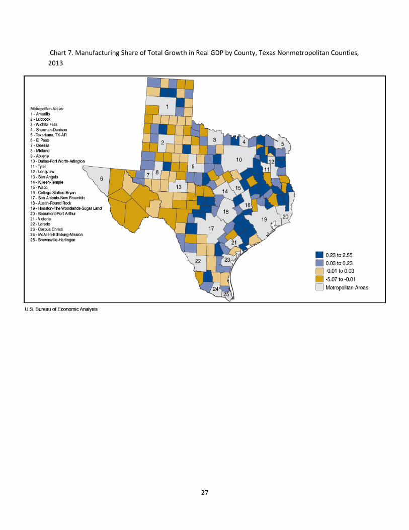
manufacturing sector are located in the eastern and northeastern parts of the state; outside the states’

largest metropolitan areas of Dallas‐Fort Worth‐Arlington, Houston–The Woodlands–Sugar Land, San

Antonio–New Braunfels, and Austin–Round Rock (chart 7). The manufacturing sector also made large

contributions to growth in non‐metropolitan counties located near the metropolitan areas of Tyler,

Longview, and Texarkana. Akin to the natural resources and mining sector, with few exceptions, this

sector either subtracted from growth or contributed very little to the GDP growth of the non‐

metropolitan counties outside this area. 11

11 Note that some of the sector contribution shares to total county GDP growth are very large due to the small size of the county’s GDP. Industry contribution shares greater than 1 (in absolute value) indicate that the industry’s contribution to growth is larger than the all industry total; the latter is the result of the growth in one industry being offset by declines in other industries.

22

Conclusions

This paper outlined the benefits of expanding BEA’s regional accounts to include GDP by county

statistics. Such benefits include providing a much richer picture of U.S. economic activity, enabling more

detailed analyses to support local resource allocation and evaluate long‐term impacts of developmental

strategies, and potentially contributing to improvements in related GDP by state and metropolitan area

statistics.

The paper also used a simple methodology to produce county GDP statistics for case studies

based on county earnings by industry that builds on the methodology of GDP by metropolitan area.

Research efforts will concentrate on improving methodologies and data sources for industries where

earnings do not provide good indicators of output or value added. For these industries, several data

sources were identified and discussed that may be used to improve measures of industry GDP. Also,

additional data sources that can help assess labor trends, business climate, and industry trends were

identified to corroborate the trends in the GDP by county statistics. A discussion of a few results from

case studies illustrated the kind of information on industry structure and local economic activity that can

be uncovered with the GDP by county statistics. Future work will include data acquisition, development

of prototype statistics, and evaluation of the results.

BEA is interested in the views of its data users on the proposed methodologies and the level of

industry detail. Please e‐mail your comments or questions to BEA at [email protected].

23

Chart 1. Quarterly Real GDP for North Dakota: Mining, Real Estate and Rental and Leasing, and Government (Millions of Chained (2009) Dollars)

Source: Bureau of Economic Analysis

Chart 2. Quarterly Real GDP for West Virginia: Mining, Real Estate and Rental and Leasing, and Government (Millions of Chained (2009) Dollars)


24

Chart 3. The Bakken Oil Reserves

Chart 4. The Marcellus Oil Reserves

25

Chart 5. Active U.S. Coal Mines

26

Chart 6. Natural Resources and Mining Share of Total Growth in Real GDP by County, Texas

Nonmetropolitan Counties, 2013

27

Chart 7. Manufacturing Share of Total Growth in Real GDP by County, Texas Nonmetropolitan Counties,

2013

28

Table 1. Per Capita Personal Income, 2014

Source Teton County, WY Lincoln County, MT

Earnings by place of work 58,819.58 14,432.42

Less: Contributions for government social insurance 7,397.73 2,191.48 Employee and self‐employed contributions for government social insurance 3,248.84 1,254.33

Employer contributions for government social insurance 4,148.89 937.15

Plus: Adjustment for residence (5,438.86) 674.04

Equals: Net earnings by place of residence 45,982.99 12,914.98

Plus: Dividends, interest, and rent 143,682.86 6,818.46

Plus: Personal current transfer receipts 4,818.75 11,262.95


Table 2. Earnings‐to‐GDP Ratios by Industry, U.S. GDP by state, 2013

Industry Name Ratio

1 All Industries 0.62

2 Private industries 0.60

3 Agriculture, forestry, fishing, and hunting 0.76

4 Mining 0.41

5 Utilities 0.32

6 Construction 0.91

7 Manufacturing 0.49

8 Wholesale trade 0.52

9 Retail trade 0.64

10 Transportation and warehousing 0.73

11 Information 0.45

12 Finance and insurance 0.61

13 Real estate and rental and leasing 0.14

14 Professional, scientific, and technical services 0.88

15 Management of companies and enterprises 0.84

16 Administrative and waste management services 0.82

17 Educational services 0.92

18 Health care and social assistance 0.94

19 Arts, entertainment, and recreation 0.70

20 Accommodation and food services 0.71

21 Other services, except government 1.03


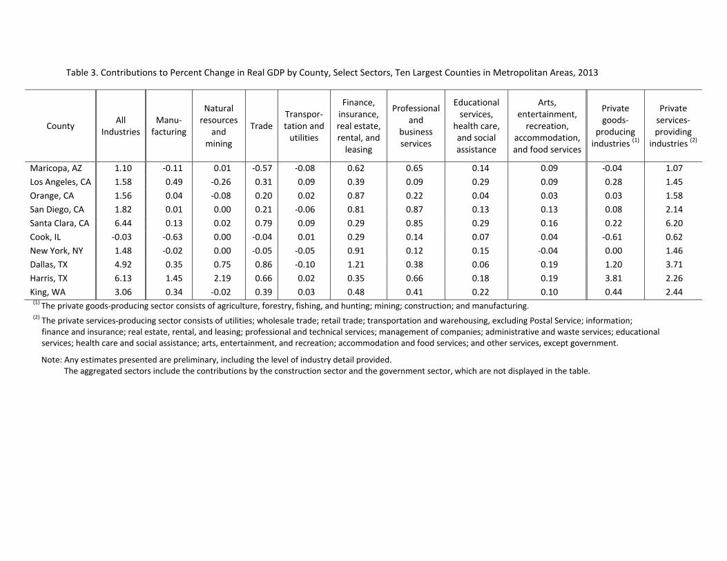
Table 3. Contributions to Percent Change in Real GDP by County, Select Sectors, Ten Largest Counties in Metropolitan Areas, 2013

County All

Industries Manu‐facturing

Natural resources

and mining

Trade Transpor‐tation and utilities

Finance, insurance, real estate, rental, and leasing

Professional and

business services

Educational services,

health care, and social assistance

Arts, entertainment, recreation,

accommodation, and food services

Private goods‐

producing industries (1)

Private services‐providing

industries (2)

Maricopa, AZ 1.10 ‐0.11 0.01 ‐0.57 ‐0.08 0.62 0.65 0.14 0.09 ‐0.04 1.07

Los Angeles, CA 1.58 0.49 ‐0.26 0.31 0.09 0.39 0.09 0.29 0.09 0.28 1.45

Orange, CA 1.56 0.04 ‐0.08 0.20 0.02 0.87 0.22 0.04 0.03 0.03 1.58

San Diego, CA 1.82 0.01 0.00 0.21 ‐0.06 0.81 0.87 0.13 0.13 0.08 2.14

Santa Clara, CA 6.44 0.13 0.02 0.79 0.09 0.29 0.85 0.29 0.16 0.22 6.20

Cook, IL ‐0.03 ‐0.63 0.00 ‐0.04 0.01 0.29 0.14 0.07 0.04 ‐0.61 0.62

New York, NY 1.48 ‐0.02 0.00 ‐0.05 ‐0.05 0.91 0.12 0.15 ‐0.04 0.00 1.46

Dallas, TX 4.92 0.35 0.75 0.86 ‐0.10 1.21 0.38 0.06 0.19 1.20 3.71

Harris, TX 6.13 1.45 2.19 0.66 0.02 0.35 0.66 0.18 0.19 3.81 2.26

King, WA 3.06 0.34 ‐0.02 0.39 0.03 0.48 0.41 0.22 0.10 0.44 2.44 (1) The private goods‐producing sector consists of agriculture, forestry, fishing, and hunting; mining; construction; and manufacturing. (2) The private services‐producing sector consists of utilities; wholesale trade; retail trade; transportation and warehousing, excluding Postal Service; information; finance and insurance; real estate, rental, and leasing; professional and technical services; management of companies; administrative and waste services; educational services; health care and social assistance; arts, entertainment, and recreation; accommodation and food services; and other services, except government.

Note: Any estimates presented are preliminary, including the level of industry detail provided. The aggregated sectors include the contributions by the construction sector and the government sector, which are not displayed in the table.

30

Table 4. Contributions to Percent Change in Real GDP by County, Select Sectors, Ten Largest Counties outside the Metropolitan Areas, 2013

County All

Industries Manu‐facturing

Natural resources

and mining

Trade

Transpor‐tation and

utilities


Professional and

business services





Private goods‐

producing industries (1)

Private services‐providing

industries (2)

North Slope Borough, AK ‐17.74 0.00 ‐17.76 0.06 ‐0.04 ‐0.09 0.00 0.06 ‐0.02 ‐17.77 0.02 Litchfield, CT 1.20 0.61 ‐0.02 0.08 0.17 0.67 ‐0.35 ‐0.23 ‐0.18 0.66 0.16

Hawaii, HI 1.30 0.06 0.10 ‐0.03 ‐0.03 ‐0.42 0.44 0.24 0.09 0.67 0.38

Wilson, NC 4.42 4.63 ‐0.10 ‐0.13 ‐0.02 0.39 0.08 ‐0.10 ‐0.05 4.45 0.29

Williams, ND 7.66 ‐0.09 2.20 0.55 0.67 1.96 0.26 0.06 0.32 3.48 3.98

Grafton, NH 1.16 0.81 ‐0.12 0.18 0.26 ‐0.06 ‐0.58 0.54 0.19 0.63 0.65

Merrimack, NH 1.31 0.21 ‐0.31 0.33 0.00 0.81 ‐0.14 0.18 0.10 0.03 1.54

Eddy, NM 8.12 1.44 5.80 0.44 0.39 0.53 ‐0.02 ‐0.21 0.07 6.99 1.28

Campbell, WY 0.34 ‐0.14 2.29 ‐0.43 ‐0.61 ‐0.10 ‐0.09 ‐0.05 0.01 1.65 ‐1.46

Sweetwater, WY 2.02 ‐0.13 2.67 ‐0.21 ‐0.31 0.47 0.02 0.03 ‐0.05 2.12 ‐0.02 (1) The private goods‐producing sector consists of agriculture, forestry, fishing, and hunting; mining; construction; and manufacturing. (2) The private services‐producing sector consists of utilities; wholesale trade; retail trade; transportation and warehousing, excluding Postal Service; information; finance and insurance; real estate, rental, and leasing; professional and technical services; management of companies; administrative and waste services; educational services; health care and social assistance; arts, entertainment, and recreation; accommodation and food services; and other services, except government.


31

Table 5. Contributions to Percent Change in Real GDP, Select Sectors, Texas, 2013

Geography All Industries Manufacturing

Natural resources

and mining

Trade


utilities


Professional and business services





Texas 5.45 1.24 1.29 0.85 ‐0.02 0.63 0.46 0.18 0.26

Metropolitan Portion 5.52 1.25 1.26 0.85 ‐0.03 0.64 0.48 0.19 0.26

Nonmetropolitan Portion 4.60 1.02 1.65 0.85 0.10 0.44 0.13 0.04 0.17


32

Table 6. Contributions to Percent Change in Real GDP, Select Sectors, Dallas‐Fort Worth‐ Arlington Metropolitan Area and Component Counties,

2013

Geography All Industries

Manu‐facturing

Natural resources and mining

Trade


utilities


Professional and business services





Dallas‐Fort Worth‐Arlington, MSA 5.28 1.00 0.66 0.94 ‐0.04 0.87 0.39 0.18 0.25

Collin 5.92 1.61 0.40 0.83 0.25 0.61 0.49 0.43 0.56

Dallas 4.92 0.35 0.75 0.86 ‐0.10 1.21 0.38 0.06 0.19

Denton 8.79 2.28 ‐0.67 2.66 0.09 1.09 0.81 0.85 0.56

Ellis 7.91 5.14 ‐0.33 1.24 0.58 0.25 ‐0.11 0.07 0.27

Hood 7.31 0.63 5.05 0.19 0.31 0.35 ‐0.17 0.27 0.53

Hunt 8.47 6.60 ‐0.15 0.46 ‐0.05 0.27 0.06 0.30 0.23

Johnson 1.32 1.17 ‐1.32 0.20 0.00 0.43 0.21 0.01 0.11

Kaufman 7.51 3.05 0.32 1.35 0.14 0.42 0.72 0.15 0.19

Parker 8.15 1.39 3.45 0.83 0.39 0.55 0.15 0.27 0.28

Rockwall 9.02 1.97 0.08 3.31 0.34 1.30 0.16 0.59 0.44

Somervell ‐7.94 0.02 0.14 0.18 ‐8.93 0.11 0.12 0.03 0.10

Tarrant 4.98 1.61 0.83 0.87 0.01 0.24 0.34 0.22 0.19

Wise 4.88 1.46 1.32 0.59 ‐0.91 0.28 0.67 ‐0.23 0.17


a research agenda for measuring gdp at the county level wp_research agenda... · a research agenda...

Documents