a remote rangeland analysis system

A Remote Rangeland Analysis System

EUGENE L. MAXWELL

Highlight: This paper describes a “now ” capability whereby satellite imagery could provide range managers with maps and tables giving standing crop biomass for selected species groups or range types (swales, uplands, etc.). This capability is provided by a remote rangeland analysis system which can monitor the effects of weather, grazing intensity, and land-management actions on primary production. The system concepts resulted from a project designed to assess the usefulness of ERTS and other remote sensing systems as sources of information for rangeland management. A field measurement program supported and verified the successful use of ER TS imagery for computer classification of vegetation type and quantity of standing crop biomass. Biomass classification was accomplished on three successive ERTS images, without changing the classification parameters, indicating that biomass classification may be less critical than expected. Extensive statistical analysis of ERTS data has shown that the MSS (multispectral scanner) Channel 5 and the ratio of Channel 7 to Channel 5 provide the most significant variables for vegetation type and biomass classifications. Cross-classification results of vegetation type and biomass provide tables summarizing biomass availability by species groups and in total acres.

Frequent monitoring of range and crop conditions is a prerequisite to effective management and planning decisions. Remote sensing can help improve such decisions by providing efficient monitoring of the quantity of standing crop biomass. This paper reports on initial efforts to develop a system to provide useful information for rangeland managers on a timely and economic basis.

The remote rangeland analysis system (RRAS) described in this paper will be of benefit to government agen- cies charged with management of pub- lic lands and to ranch managers. Ap- plication to the grasslands of the entire world may be possible.

A conceptual description of the RRAS is followed by a discussion of the theoretical basis for remote sensing of vegetation, taken mostly from work by Miller and Pearson (1971) and Tucker (1973). An important part of the complete system includes algo- rithms and computer programs for performing pattern recognition type analyses. The brief summary of these methods will help the reader who has not previously used them. A description of the experimental program includes a discussion of the collection of field data used to verify the analysis of remote sensing imagery. The experi-

The author is associate professor, De- partment of Earth Resources, Colorado State University, Fort Collins.

This paper reports on work supported by the U.S. Geological Survey-Contract No. 14-08-0001-13561.

Manuscript received January 29, 1975.

66

INPUT

Soils

Vegetation Climate

Topography

Precipitation

Max-Min Temp.

OUTPUT

Species

mental results provide a quantitative analysis of the accuracy with which remote sensing data may be used to interpret range conditions. Particular emphasis was given to the recognition or classification of the quantity of standing crop biomass. Finally, the management implications of the RRAS system are discussed.

System Concepts

Some initial design concepts of a complete remote rangeland analysis system are shown in Figure 1. To date, only the ERTS analysis program has

INPUT

ERTS Imagery

Soils

Topography

Spectroreflectance Data

Species

Phenology

Weather Effects

f Phenology

Weather Effects

OUTPUT

Biomass

A Biomass

Species Groups

Phenology

Fig. 1. Conceptual description of a remote rangeland analysis system.

JOURNAL OF RANGE MANAGEMENT 29(l), January 1976

60

(From Pearson and Niller, 1972)

50

10

0.4 0.5 0.6 0.7 0.8 WAVELENGTH, urn

Fig. 2. Spectroreflectance of soil, dead vegetation, and green vegetation.

been implemented. The results of our research, however, have shown the need for a “simplified range model” which would perform the functions indicated in the diagram. In short, reliable analysis of ERTS imagery re- quires some prior knowledge of species, phenological changes, and effects of weather. We found, for in- stance, that correct biomass classification for fourwing saltbush (AtripZex canescens) must include the effect of flowering on the spectral reflectance characteristics of this species. The simplified range model would also be used to predict probable species groups and to estimate weather effects on soil moisture. The preanalysis pre- diction of species groups or eco- systems would minimize ground sur- veys. The primary need for species and phenology information is due to the different biomass and reflectance characteristics for different species and different phenological states.

Our experimental operation of the RRAS made use only of the ERTS analysis program. The operation of the simplified range model was simulated by on-the-ground identification of species groups and phenological states. Thus the results reported in this paper incorporated the operation of the ERTS analysis program and the simu- lation of the simplified range model.

The Basis for Remote Sensing Biomass

The combined effect of biomass quantity, chlorophyll, and leaf water content must be considered, because for a given species or species group they are highly correlated. If there is more biomass of a given species, there will be more chlorophyll and more leaf water. Tucker (1973) has shown a high interdependence among these parameters and high correlations of each with the spectral reflectance of plants. 2

The spectral reflectances of soil, dead vegetation, and green vegetation are shown in Figure 2. These results taken from Pearson and Miller (1972), indicate that a remote sensing system should be capable of differentiating between green vegetation and under- lying materials. Thus, a system capable of detecting the electromagnetic radiation from plants will provide a measurement related to biomass, chlorophyll, and leaf water. These parameters could be combined into a single parameter, wet-green-biomass. By definition, wet-green-biomass includes leaf water, chlorophyll, and biomass. This parameter was chosen to obtain the results contained herein.

More detailed informat ion relative to the physiochemical relationships between these parameters and leaf reflectance may be obtained from Knipling (1970), Carlson (197 l), Carnenas and Gausman (1971) and Gausman et al. (197 1).

Methods and Procedures

Pattern Recognition

Pattern recognition procedures provide for the recognition of or discrimi- nation between specified groups or classes, defined as multivariate, normally distributed populations represented by data samples. Each population can be described mathe- matically by its mean vector-,&i, and its covariance matrix, &Ii. In this in- stance, the mean vector consists of average reflectance values for each ERTS band. The covariance matrix provides a measure of the scatter of

Class A

Fig. 3. Data groups (populations) in three dimensional space. Ellipsoids represent the covariance boundaries.

JOURNAL OF RANGE MANAGEMENT 29(l), January 1976 67

data around the means. In effect, these two parameters establish a signature for each class. If the variates are only three in number, we may pictoually represent these data groups as shown in Figure 3.

Pattern recognition methods are designed to determine to which ellip- soid (identified by /“i and Ci) each data sample belongs. This is accomplished by using the conditional probability density function (f(Xj/Ci)) for each class, i. This function’ deter- mines the probability that sample xjbelongs to class Ci. The decision Lo classify a sample point xj ds class I

rather than class 2 is made according LO the equation

f(Xj/Cl 1 __ > 1 (dmde class 1) (1) f(xj(c* 1

This is the classification method USed for this research.

One must recognize that the mean vectors and covariance matrices for the classes are not usually known. They are computed from sample reflectance data for the classes. This sample data is usually called “training data” in the sense that It is used to “train” the computer to recognize the classes.

Experimental Program

The primary objective of the experimental program was the measurement of range conditions in se&ted test fields. ERTS reflectance data from these test fields could then be used as training data for calculating p and 4 values. The Lest fields, or combinations thereof, become the classes to be identified. A measurement program was set UD to accomolish the followiw objectives.

1) Establish test sites representing different rangeland conditions, species groups, and biomass quantities.

2) Maintain a record of atmos- pheric and ground conditions at the time of each ERTS overflight.

3) Obtain a quantitative record of actual range conditions within each test field in terms of canopy cover, biomass, and phenological change.

Most of the test fields used on this effort are shown on Figure 4, which is an aerial (aircraft) photograph of part of the Pawnee National Grasslands in northeastern Colorado. This is the location of the International Biological

Table 1. Green biomass data for Site 2, LBOGR on August 15, 1973.

Species abbreviation Common name

Biomass lb/acre

ATCA Fourwing Saltbush 58 OPPO Plains Pricklypear 1,235 ARFR Fringed Sagewort 218 ARLO Red Threeawn 174 BAOP Plains Bahia 11 BOGR Blue Grama 591 BUDA Buffalo Grass 127 CAEL Needleleaf Sedge 78 MUTO Ring Muhly 9 SIHY Bottlebrush Squirreltail 123 SPCO Scarlet Globemallow 71 SPCR Sand Dropseed 20 OTHER Other 20

Total bioma ss 2,735

Program (IBP) grassland biome site. The vegetation is typical of the shortgrass prairie of the great plains. Blue grama (Bouteloua gracilis) is the dominant grass species accounting for 75% of the weight of gramineous vegetation. The vegetation classes which were monitored for canopy cover, biomass, and phenological change in- cluded a heavily grazed blue grama field, HBOGR; a lightly grazed blue grama field, LBOGR; a pitted blue grama field, PITTED;a western wheatgrass (Agropyron smithii) swale, ASWALE; a crested whea tgrass (Agropyron d eser torum) field, CRESTD; and a fourwinged saltbush area, FRWING. All but the crested wheatgrass field are shown on Figure 4.

Sampling of vegetation for the July 10, July 28, and August 15, 1973, ERTS overpass dates followed a sys- tematic procedure. Circular quadrats, 1,000 square centimeters in area, were used in a double sampling procedure to estimate canopy cover and green standing crop biomass of each species. The double sampling procedure in- cluded ocular estimates of canopy cover and green biomass and clipping and weighing of all vegetation in every fifth plot. A regression analysis was then used to correct the ocular estimates of biomass. Twenty quadrats were sampled within each of three stands for each of the test fields. An example of the reduced and corrected biomass data is given in Table 1 for the lightly grazed blue grama field on August 15, 1973. Similar measurement data were obtained for all of the six grassland fields for each of the three dates noted above.

Three additional test sites were used for classification purposes but were not sampled for biomass. These include the sandy arroyo, SAND, shown on Figure 4, which was ob- served to have almost no vegetation of any type. Wheat fields, WHEAT, were

used to form Test Site 8 and the fallow ground, GROUND, between the wheat fields was designated Test Site 9. Since dryland wheat fields are com- monly found near grassland areas, their classification was important.

The spring and early summer of 1973 were unusually dry in northeastern Colorado. Growth-inducing rains did not occur in the Pawnee area until after July 10. Between July 15 and August 15, several one-half to one-inch rains occurred, which resulted in significant changes in biomass. Computer compatible tapes (digital image data) were obtained from the EROS Data Center for July 10, July 28, and August 15, 1973. The selection of training data from the computer compatible tapes was accomplished in three steps. Data for the Pawnee Test Site were selected and

displayed on computer microfilm and page print outputs. An ERTS computer microfilm image of the Pawnee Test Site for July 10, 1973, is shown on Figure 5, where roads and test fields are easily seen. Next, data for specific picture elements (pixels) were selected from the test field locations for each of the three dates in July and August. Each dot on Figure 5 is a pixel, 1 .l acres in size. If these were homogenous fields, such as one would find for agricultural crops, this would have completed the selection of training data. Natural grassland fields are not homogenous, however, so data samples which were significantly different from the majority of the class were removed. Significant difference was determined by calculating conditional probabilities (p(xjlCi)). This completed the selection of training data.

Red ts

The ERTS MSS (Multispectral scan- ning) imaging system measures reflectance in four spectral bands, 4 through 7. The wavelengths measured are 0.5 to 0.6, 0.6 to 0.7, 0.7 to 0.8, and 0.8 to 1 .l micrometers. In addition to the four MSS bands, the ratio of Band 7 to Band 5 was also used. The use of this ratio was based on the spectroreflectance characteristics of green vegetation as illustrated in Figure 2. Increasing quantity of vegetation (biomass) will reduce the reflectance in

Fig. 5. Computer microfilm image of part of the Pawnee Test Site (July 10, 1973-ENTS Channel 7).


Band 5 since this band includes the chlorophyll absorption band. On the other hand, increasing biomass will increase the reflectance in Band 7 due to the high reflectance of green vegetation in the near infrared. Thus, the ratio of these two bands will increase as biomass increases. An analysis of variance procedure verified the importance of this ratio.

Vegetation Type Classification

A stepwise discriminant computer program was used to classify the training data (ERTS) for the nine test sites. This program established the capability of the Bayesian classification method to recognize these fields. It also determined the relative importance of each of the variables.

The classification results for the training field data for August 15, 1973, are given in Table 2. Somewhat better results were obtained for the other two dates, but these are repre- sentative. The 7.7% average error in- dicates classification results should be reliable. The dominant variables accounting for most of the separation between classes were ERTS Band 5 and the ratio 7/5, in that order.

The training data were then used to compute mean vectors and covariance matrices (signatures) for each of the test field classes. These vectors and matrices were used with Colorado State University‘s pattern recognition program (RECOG) to classify the entire area within the Pawnee Test Site. The results of this classification are shown in Figure 6. The classifications shown pictorially in Figure 6 were stored on computer tape for later use. These results are consistent with known field boundaries for this region. The size of the region and its hetero-

Fig. 6. Classification map of vegetation types for the Pawnee Test Site-August IS, 1973. (A parity error caused the white streak.) Classes from black to white are: GROUND, SAND, WHEAT, CRESTD, PITTED, HBOGR, LBOGR, ASWALE, FRWING, NOT CLASSIFIED.

geneity precluded any assessment of classification accuracy.

Biomass Classification

The formation of training data for biomass classes was based upon the field measurements of biomass at the time of each ERTS overpass. The biomass classes were formed as shown in Table 3. Notice that ERTS data from test fields having different species groups and data obtained from images of different dates were combined. The biomass of the pricklypear cactus (OPPO) was excluded from measured values of total green biomass because of its inordinately high biomass/surface area ratio. Data for the

Table 2. Number of cases classified into each vegetation class for test site training data, August 15, 1973.

Vegetation class’ 1 2 3

Vegetation class

4 5 6 7 8 9 Percent errors

1. HBOGR 62 9 3 0 0 0 0 0 0 16 2. LBOGR 9 75 0 0 2 0 0 0 0 13 3. PITTED 0 0 38 0 0 2 0 0 0 5 4. FRWING 0 0 0 47 2 0 0 0 0 4 5. ASWALE 0 2 0 0 38 0 0 0 0 5 6. CRESTD 0 0 2 0 0 18 0 0 0 10 7. SAND 0 0 0 0 0 0 21 0 1 5 8. WHEAT 0 0 1 0 0 2 0 41 0 7 9. GROUND 0 0 0 0 0 1 0 0 22 4

Average 7.7

’ HBOGR = heavily grazed blue grama field; LBOGR = lightly grazed blue grama field; PITTED = blue grama field; FRWING = fourwinged saltbush area; ASWALE = western wheatgrass swale; CRESTD = crested wheatgrass field; SAND = sandy arroyo; WHEAT = wheat fields; and GROUND = fallow ground.

70 JOURNAL OF RANGE MANAGEMENT 29(l), January 1976

biomass classes were used without any change except for fourwing saltbush data for July 10. These data were modified slightly to compensate for the reflectance of profuse blooms which were present on that date.

Stepwise discriminant classification results for the biomass training data are given in Table 4. The relatively high average classification error of 24.6% can be attributed to the limited biomass sampling program and natural variation of biomass within the test fields. This is indicated by the more or less uniform distribution of errors around the “true” values (47% of the errors are for biomass classes higher than “true” values, 53% are for lower values). Thus, many of the “errors” are not wrong classifications, but are the result of actual biomass variations in fields placed in fixed biomass classes. An accurate estimation of biomass classification accuracy would require extensive sampling for each 1 .l-acre picture element imaged by ERTS.

The most significant variables for biomass classification were the ratio 7/5 and Band 5, in that order.

Mean vectors and covariance matrices were computed for the biomass classes and used to classify the Pawnee Test Site as shown in Figures 7 and 8. Recalling that most of the

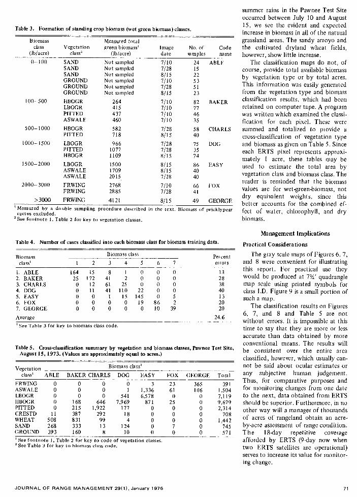
Table 3. Formation of standing crop biomass (wet green biomass) classes.

Biomass class

(lb/acre) Vegetation

class’

Measured total green biomass’

(Ib/acre) Image No. of Code date samples name

O-100

100-500

500- 1000

1 ooo- 1500

1500-2000

2000- 3000

SAND SAND SAND GROUND GROUND GROUND

HBOGR LBOGR PITTED ASWALE

HBOGR PITTED

LBOGR PITTED HBOGR

LBOGR ASWALE ASWALE

FRWING FRWING

Not sampled Not sampled Not sampled Not sampled Not sampled Not sampled

264 415 437 460

582 718

966 1077 1109

1500 1709 2015

2768 2885

7/10 7128 S/15 7/10 7128 8115

7/10 7/10 7/10 7/10

7128 8115

7128 7128 8115

8/15 8115 7128

7/10 7128

24 ABLE 15 22 53 51 23

82 BAKER 77 46 35

58 CHARLS 40

75 DOG 35 74

86 EASY 40 40

66 FOX 41

>3000 FRWING 4121 8/l 5 49 GEORGE ‘Measured by a double sampling procedure described in the text. Biomass of pricklypear

cactus excluded. 2 See footnote 1, Table 2 for key to vegetation classes.

Table 4. Number of cases classified into each biomass class for biomass training data.

Biomass class’ 1 2

Biomass class Percent 3 4 5 6 7 errors

1. ABLE 164 15 8 1 0 2. BAKER 25 172 41 2 0 3. CHARLS 0 12 61 25 0 4. DOG 0 11 41 110 22 5. EASY 0 0 1 15 145 6. FOX 0 0 0 0 19 7. GEORGE 0 0 0 0 0

Average

’ See Table 3 for key to biomass class code.

0 0 13 0 0 28 0 0 38 0 0 40 0 5 13

86 2 20 10 39 20

24.6

Table 5. Cross-classification summary by vegetation and biomass classes, Pawnee Test Site, August 15, 1973. (Values are approximately equal to acres.)

Vegetation Biomass class2

class’ ABLE BAKER CHARLS DOG EASY FOX GEORGE Total

FRWING 0 0 0 0 3 23 365 391 ASWALE 0 0 0 1 1,336 61 106 1,504 LBOGR 0 0 0 541 6,578 0 0 7,119 HBOGR 0 168 646 7,969 871 25 0 9,679 PITTED 0 215 1,922 177 0 0 0 2,314 CRESTD 11 387 292 18 0 0 0 708 WHEAT 508 831 99 4 0 0 0 1,442 SAND 268 333 13 124 0 7 0 745 GROUND 393 160 8 10 0 0 0 571

’ See footnote I, Table 2 for key to code of vegetation classes. 2 See Table 3 for key to biomass class code.

summer rains in the Pawnee Test Site occurred between July 10 and August 15, we see the evident and expected increase in biomass in all of the natural grassland areas. The sandy arroyo and the cultivated dryland wheat fields, however, show little increase.

The classification maps do not, of course, provide total available biomass by vegetation type or by total acres. This information was easily generated from the vegetation type and biomass classification results, which had been retained on computer tape. A program was written which examined the classification for each pixel. These were summed and totalized to provide a cross-classification of vegetation type and biomass as given on Table 5. Since each ERTS pixel represents approximately 1 acre, these tables may be used to estimate the total area by vegetation class and biomass class. The reader is reminded that the biomass values are for wet-green-biomass, not dry equivalent weights, since this better accounts for the combined effect of water, chlorophyll, and dry biomass.

Management Implications

Practical Considerations

The gray scale maps of Figures 6, 7, and 8 were convenient for illustrating this report. For practical use they would be produced at 7%’ quadrangle map scale using printed symbols for class I.D. Figure 9 is a small portion of such a map.

The classification results on Figures 6, 7, and 8 and Table 5 are not without errors. It is impossible at this time to say that they are more or less accurate than data obtained by more conventional means. The results will be consistent over the entire area classified, however, which usually can- not be said about ocular estimates or any subjective human judgement. Thus, for comparative purposes and for monitoring changes from one date to the next, data obtained from ERTS should be superior. Furthermore, in no other way will a manager of thousands of acres of rangeland obtain an acre- by-acre assessment of range condition. The 18-day repetitive coverage afforded by ERTS (9-day now when two ERTS satellites are operational) serves to increase its value for monitoring change.


Fig. 7. Biomass classification map for the Pawnee Test Site-July 10, 1973. Biomass classes from black to white are: >3,000 lb/acre, 2,000 to 1,000 to 1,500 lb/acre, 500 to 1,000 lb/acre, 100

3,000 lb/acre, 1,500 to lb/acre, 2,000 to 500 lb/acre, 0 to 100 lb/acre, not

classified. (This is wet green biomass.)

1

Fig. 8. Biomass classification map for the Pawnee Test Site-August 15, 1973. (A parity error caused the white streak.) Biomass classes from black to white are: >3,000 lb/acre, 2,000 to 3,000 lb/ acre, 1,500 to 2,000 lb/acre, 1,000 to 1,500 lb/acre, 500 to 1,000 lb/acre, 100 to 500 lb/acre, 0 to IO0 lb/acre, not classified. (This is wet green biomass.)

Fig. 9. Vegetation classification for a small portion of the Pawnee Test Site-July 28, 1973. The original of this symbol I.D. map would be at 1:24,000 scale. Each symbol represents about I.2 acres. Shown here is the south end of Site 4 (F), part of the sandy arroyo (S), part of Site 3 (P), a heavily grazed blue grama field (H), and a nondescript area south and east of Site 4.

My personal confidence in the po- tential for a RRAS must be tempered by consideration of some of the problems. First and foremost is the prob- lem of cloudy weather. Heavy clouds totally obscure the ground and elimi- nate all data. Thin clouds such as cirrus upset classification and greatly decrease the reliability of results. Simi- larly, precipitation a day or two before imaging can change soil reflectance and, therefore, total scene reflectance. The presence of even thin clouds is usually obvious, so unreliable data can be identified as such. A localized rain storm might not be recorded and will not likely be noted on the imagery. Hence, the effect of recent precipitation may be more serious. Further- more, a functional RRAS will require some sort of simplified range model as depicted in Figure 1. Such a model is not presently available; thus we are dependent on some ground control information on species, phenology, and weather effects (such as the precipitation effect just noted). Finally, a present limitation on availability of imagery limits operational use. It usually takes about 2 months after the image date to obtain computer com-

72 JOURNAL OF RANGE MANAGEMENT 29(l), January 1976

patible tapes. There is good reason to believe

these problems can be solved or at least ameliorated. This can be best accomplished by research coupled with operational experience. Only from the results of routine operation will we gain a complete understanding of the capability and limitations of remote sensing. And of course, only by using it will range managers gain confidence in the information provided.

Economics

The economics of operating a RRAS are encouraging but quite vari- able. The cost of computer compatible tapes for a 115mile by 115-mile image is $200.00. This is minor if even a tenth of the area is rangeland. For a lo-square-mile region, however, it could be excessive. And at the present time, a user must purchase tapes for an entire image or none at all. This points to the need for collective use.

The cost of classifying a 1 ,OOO- square-mile region (acre by acre) using Colorado State University’s computer is approximately $2,000.00. Com- bining 3 X 3 squares of 9 pixels into lo-acre cells, however, will reduce this cost to about $500.00. Furthermore, computers 100 times faster are available, which would reduce these costs by a factor of 10 to 50, depending on the computer and its owner. In the final analysis, cost will not be a deter- rent if the data provided are reliable and timely.

Summary and Conclusions

The most significant results from this research are: (1) the successful use of the computer to recognize vegetation type-range conditions and green biomass classes, (2) achieving good statistical separation of the above classes, (3) the use of mixed date and mixed species data for “training” the computer to recognize biomass classes. The species and biomass classes are not, of course, entirely unique or independent. Species and range condition classifications were correlated to biomass differences in the fields.

The output in the form of maps and cross-classification tables will provide useful information for the rangeland manager. This is a “now” capability which could be economically applied, at least in the shortgrass prairies, on a routine basis for rangeland management. Because of present delays of up to 2 months in obtaining ERTS imagery, however, its use at the present time would have to be limited to an inventory type function. Some limitations on its use would also be imposed by weather and the need for a simple range model to complete the analysis system.

Future research should be per- formed in other locations, having different grass species, to determine the extent to which these results may be applied to other areas. There is some evidence that classification parameters for grassland biomass may be relatively

universal. Development and operation of the entire remote rangeland analysis system should have a high priority for future efforts.

Literature Cited Cardenas, R., and H. W. Gausman. 1971.

Light reflectances, chlorophyll assays and photographic film densities of iso- genie barley lines. Spectral survey of irrigated crops and soils annual report. Agr. Res. Serv., U.S. Dep. Agr., We&co, Texas. V. I. 36-V, I. 40.

Carlson, R. E. 1971. Remote detection of moisture stress: Field and laboratory experiments. PhD Thesis. Iowa State Univ., Ames, Iowa. 101 p.

Gausman, H. W., W. A. Allen, C L Wiegand, M. Schupp, D. E. Escobar, and R. R. Rodriguez. 1971. Leaf light reflectance, transmittance, absorptance, and optical and geometrical parameters for eleven plant genera with different leaf mesophyll arrangements. Seventh Int. Symp. on Remote Sensing of Environ., Univ. of Mich., Ann Arbor, Mich.

Knipling, E. B. 1970. Physical and physio- logical basis for the reflectance of visible and near infrared radiation from vegetation. Remote Sensing of Environ. 1:155-159.

Miller, L D., and R. L Pearson. 1971. Aerial mapping program of the IBP Grassland Biome: Remote sensing of the productivity of shortgrass prairie as input into biosystem models. Proceedings of the 7th Int. Symp. on Rem. Sens. Vol. I, Univ. of Mich. p. 165-207.

Pearson, R. L., and L. D. Miller. 1972. Remote spectral measurements as a method for determining plant cover. Int. Biol. Program. Tech Rep. No. 167, Colo. State Univ., Sept., 1972.

Tucker, C J. 1973. The remote estimation of a grassland canopy. MS Thesis, Colo- rado State Univ., Fort Collins.

a remote rangeland analysis system

Documents