a rapidly convergent approximation method for …ijseas.com/volume2/v2i8/ijseas20160833.pdf · a...

International Journal of Scientific Engineering and Applied Science (IJSEAS) – Volume-2, Issue-8, August 2016 ISSN: 2395-3470

www.ijseas.com

334

A Rapidly Convergent Approximation Method for Nonlinear Ordinary Differential Equations

Prakash Kumar Das, M.M. PanjaP

1

Department of Mathematics, Visva-Bharati, Santiniketan 731 235, West Bengal, India [email protected], [email protected]

P

1PCorresponding author

Abstract

This paper deals with an approximation scheme for getting rapidly convergent approximate solution of some nonlinear ordinary or partial differential equations appearing in the mathematical analysis of physical processes. Here the solutions are expressed in a series of exponential functions rather than the series of the independent variables. As a result the vanishing boundary conditions for localized solutions can be incorporated into the theory in rather straight forward way. For many cases, sum of the terms in the approximate solution can be found easily, thus provides exact analytic solution to the problem. To illustrate the efficiency and versatility of the method, proposed schemes developed here for bounded and unbounded region have been applied to some problems and have been compared with solutions obtained by some other approximation method now available. It appears that the present method is efficient, user-friendly and easy to implement through any symbolic computation software now readily available. Keywords: Nonlinear ordinary/partial differential equation, travelling wave solution, non-smooth solution, rapidly convergent approximate solution. 1. Introduction In many branches of science and engineering evolution of physical processes are described by nonlinear ordinary or partial differential equations (ODEs/PDEs). The solutions of such equations helps one visualize the nature of evolution of the processes involved. But in many cases it is not possible to find exact solution to these equations. Despite that there exists a vast amount of literature for constructing exact solutions of ODEs and PDEs [1, 2, 3, 4]. Also there are many approximation methods [5, 6, 7, 8, 9] to deal with equations for which the analytical methods do not work. In any such method the main interest is to develop a scheme that yields a physically meaningful solution with minimum computational effort. The effort expended is assessed in terms of the ease of implementation and computer resources required. Among various approximation techniques for solving nonlinear boundary value problems(BVP), the Adomian decomposition method often abbreviated as ADM enjoys a great deal of popularity because of its conceptual simplicity and usefulness in dealing with nonlinear problems [9, 10, 11, 12, 13, 14, 15, 16, 17, 18, 19, 20, 21]. In the traditional formulation of the ADM, approximate solution of any given nonlinear differential equation is expressed as a sum of functions with the leading term as a polynomial in the independent variable of the equation. These functions are often found to be slowly convergent. It appears that there is still another inherent limitation of the approach. For example, it is not straightforward to incorporate the infinite domain boundary conditions in solving the nonlinear equation by the ADM. To accommodate the boundary condition at ±∞ one needs to take recourse to the use of rational Padé approximants to express the successive terms in the approximate solution. Naturally, the question arises as to whether one can look for an improved form of the ADM which, on the one hand, will improve on the convergence of the series representing the approximate solution and, on the other hand, will incorporate the infinite domain boundary conditions of the problem. The present work is an effort in this direction. We have, in this work derived a recursive scheme for solving nonlinear boundary-value problems by seeking a modification of the conventional ADM. The modification sought by us consists in introducing a more general form of the two-point boundary-value problem than that is used in the conventional ADM to develop the algorithms to solve any nonlinear differential equation. Here the inverse of the linear operator associated with the nonlinear equation is given by a twofold integral operator involving exponentials of the independent variable rather than being dependent on the independent variable as in the case of conventional ADM. The exponential dependence of the inverse operator is the source of rapid convergence of the method proposed. Further this dependence also allows us to incorporate into the theory the infinite domain boundary conditions in a rather natural way. In section 2 we present brief review for the conventional ADM with a view to gain some feeling for the working principle of the method. We then introduce in section 3 a general nonlinear differential equation for the two-point

mailto:[email protected]

mailto:[email protected]


www.ijseas.com

335

boundary value problem and make use of it to derive the algorithms for the rapidly convergent approximate solution to the problem. The results presented are very suitable to deal with problems in bounded domain. To adapt these algorithms to treat problems in unbounded domains some modification is desirable. The desired modifications have been described in section 4. We present in sec.5 a number of case studies and thereby demonstrate the efficiency of our scheme developed here. In section 6 we have summarized our outlook on the present work and try to make some concluding remarks have been presented.

2. Salient steps of ADM For the two point boundary value problem

𝑦′′(𝑥) − 𝜆2𝑦(𝑥) = 𝑁[𝑦](𝑥) + 𝑔(𝑥) (1) within Ω = {𝑥:𝑎 ≤ 𝑥 ≤ 𝑏} subject to Dirichlet boundary conditions (DBCs)

𝑦(𝑎) = 𝛼, 𝑦(𝑏) = 𝛽 (2) one assumes that 𝑁[𝑦] is analytic in 𝑦 and contains all nonlinear terms. The inhomogeneous or source term 𝑔(𝑥) is continuous over Ω. To find the solution of (1) and (2) by using ADM [10] one recasts (1) in operator form

𝐿[𝑦](𝑥) = 𝜆2 𝑦(𝑥) + 𝑁[𝑦](𝑥) + 𝑔(𝑥) (3) where 𝐿[⋅](𝑥) = 𝑑2

𝑑𝑥2[⋅](𝑥) is a second-order linear differential operator so that its inverse can be found as

𝐿−1[⋅](𝑥) = ∫ 𝑥𝑎 ∫ 𝑥′𝑎 [⋅](𝑥′′) 𝑑𝑥′′ 𝑑𝑥′, 𝑥 ∈ Ω. (4)

Operating 𝐿−1 on 𝐿[𝑦](𝑥) for 𝑦 ∈ 𝐶2(Ω) and following integration by parts one gets

𝐿−1[𝐿[𝑦]](𝑥) = 𝑦(𝑥) − 𝑦(𝑎) − 𝑦′(𝑎)(𝑥 − 𝑎). (5) Applying operator 𝐿−1 on both sides of (3) and using the result of (5), one gets the solution

𝑦(𝑥) = 𝑦(𝑎) + 𝑦′(𝑎)(𝑥 − 𝑎) + 𝜆2 𝐿−1[𝑦](𝑥) + 𝐿−1[𝑁[𝑦]](𝑥) + 𝐿−1[𝑔](𝑥) (6) which involves an unknown term 𝑦′(𝑎). To eliminate this unknown we substitute 𝑥 = 𝑏 in Eq. (6) and solve for 𝑦′(𝑎), to get

𝑦′(𝑎) = 1𝑏−𝑎

{𝑦(𝑏) − 𝑦(𝑎) − 𝜆2 𝐿−1[𝑦](𝑏) − 𝐿−1[𝑁[𝑦]](𝑏) − 𝐿−1[𝑔](𝑏)}. (7) Substitution of 𝑦′(𝑎) into (6) gives the solution 𝑦(𝑥) involving 𝐿−1 operator as

𝑦(𝑥) = 𝑦(𝑎) +1

𝑏 − 𝑎�𝑦(𝑏) − 𝑦(𝑎) − 𝜆2 𝐿−1[𝑦](𝑏) − 𝐿−1�𝑁[𝑦]�(𝑏) − 𝐿−1[𝑔](𝑏)�(𝑥 − 𝑎)

+𝜆2 𝐿−1[𝑦](𝑥) + 𝐿−1[𝑁[𝑦]](𝑥) + 𝐿−1[𝑔](𝑥). (8) To evaluate terms involving the unknown 𝑦(𝑥) in R.H.S of (8), one writes

𝑦(𝑥) = ∑ ∞𝑚=0 𝑦𝑚(𝑥) (9)

and recasts the nonlinear term into 𝑁[𝑦](𝑥) = ∑ ∞

𝑚=0 𝐴𝑚(𝑦0(𝑥),𝑦1(𝑥),⋯ ,𝑦𝑚(𝑥)). (10) Here the terms 𝐴𝑚(𝑥) = 𝐴𝑚(𝑦0(𝑥),𝑦1(𝑥),⋯ ,𝑦𝑚(𝑥)). are known as Adomian polynomials extracted from nonlinear term by using the formula [9, 10, 11, 12, 13, 14]

𝐴𝑚(𝑥) = 1𝑚!

[ 𝑑𝑚

𝑑𝜀𝑚𝑁(∑ ∞

𝑘=0 𝑦𝑘𝜀𝑘)]𝜀=0, 𝑚 ≥ 0 (11) proposed by Adomian and Rach in their seminal work in Ref.9. It is important to note here that the laborious calculations for getting 𝐴𝑚[𝑁[𝑦]](𝑥) successively can be easily executed in MATHEMATICA through the following statement:

(* Calculating Adomian polynomial 𝑨𝒏(𝒙) of (11) *) A[n_,x_]:=Module[{NL,A}, ys[z_]:=∑ 𝒏

𝒊=𝟎 yy[i,x]𝒛𝒊; NL[y_,yp_]:=#; Expand�𝟏

𝒏!(D[NL[ys[z],D[ys[z],x]],{z,n}])/.𝒛 → 𝟎]

]& In ADM, the leading approximation has been taken as the solution of 𝐿[𝑦](𝑥) = 𝑔(𝑥) satisfying boundary condition (2)


www.ijseas.com

336

𝑦0(𝑥) = 𝑦(𝑎) + 𝑦(𝑏)−𝑦(𝑎)−𝐿−1[𝑔](𝑏)𝑏−𝑎

(𝑥 − 𝑎) + 𝐿−1[𝑔](𝑥). (12) Here the terms involving conditions on the boundry is a first order polynomial in (𝑥 − 𝑎). The successive terms in the expansion (9) for 𝑦(𝑥) can then be obtained recursively by using the formula

𝑦𝑛+1(𝑥) = 𝜆2𝐿−1[𝑦𝑛](𝑥) − 𝜆2 𝐿−1[𝑦𝑛](𝑏)+𝐿−1[𝐴𝑛](𝑏)𝑏−𝑎

(𝑥 − 𝑎) + 𝐿−1[𝐴𝑛](𝑥), (13) for 𝑛 ≥ 0. It is important to mention here that whenever the domain becomes infinite i.e., [0,∞) or (−∞,∞), 𝑦′(𝑎) appearing in the formula (6) cannot be determined in a straightforward way due to presence of the factor (𝑥 − 𝑎) multiplying 𝑦 ′(𝑎). In order to resolve such problem we assemble all linear terms involved in the equation into the operator 𝐿 to get a more accurate and physically meaningful leading order approximation of the solution to the problem as described in the following section. 3. Proposed scheme for bounded domain [𝒂,𝒃] Instead of considering (1), we consider a more general equation

𝑦′′(𝑥) − (𝜆1 + 𝜆2) 𝑦′(𝑥) + 𝜆1𝜆2 𝑦(𝑥) = 𝑁[𝑦](𝑥) + 𝑔(𝑥) (14) with the same boundary condition as given in (2). Instead of including the linear term 𝜆2𝑦(𝑥) of Eq.(1) into R.H.S in ADM, we incorporate it into the operator 𝑂[⋅](𝑥) = 𝑑2

𝑑𝑥2[⋅](𝑥) − (𝜆1 + 𝜆2) 𝑑

𝑑𝑥[⋅](𝑥) + 𝜆1𝜆2[⋅](𝑥) ≡ ( 𝑑

𝑑𝑥−

𝜆2)( 𝑑𝑑𝑥− 𝜆1)[⋅](𝑥), so that Eq.(14) can now be recast into the form

𝑂[𝑦](𝑥) = 𝑁[𝑦](𝑥) + 𝑔(𝑥), 𝑎 ≤ 𝑥 ≤ 𝑏. (15) The linear operator 𝑂[⋅] can be written in the form

𝑂[⋅](𝑥) = 𝑒𝜆2𝑥 𝑑𝑑𝑥

(𝑒(𝜆1−𝜆2)𝑥 𝑑𝑑𝑥

(𝑒−𝜆1𝑥[⋅])) (16) which plays a key role in expressing the solution in terms of rapidly convergent series of exponentials. One may reinterpret the inverse operator 𝑂−1 as a twofold integral operator given by

𝑂−1[⋅](𝑥) = 𝑒𝜆1𝑥 ∫ 𝑥𝑎 𝑒(𝜆2−𝜆1)𝑥′ ∫ 𝑥′

𝑎 𝑒−𝜆2𝑥′′[⋅](𝑥′′) 𝑑𝑥′′ 𝑑𝑥′. (17) It is important to note here that representing inverse of a linear operator with variable coefficients by integrals is also possible whenever it is factorable. That operation of 𝑂−1 on LHS of (14) leads to

𝑂−1[𝑦′′(𝑥) − (𝜆1 + 𝜆2)𝑦′(𝑥) + 𝜆1𝜆2𝑦(𝑥)]

= 𝑒𝜆1𝑥 � 𝑥

𝑎𝑒(𝜆2−𝜆1)s �

𝑠

𝑎𝑒−𝜆2t(𝑦′′(t) − (𝜆1 + 𝜆2)𝑦′(t) + 𝜆1𝜆2𝑦(t)) 𝑑𝑡 𝑑𝑠

= 𝑒𝜆1𝑥 ∫ 𝑥𝑎 {𝑒−𝜆1s(𝑦′(s) − 𝜆1𝑦(s)) − 𝑒−𝜆2𝑎𝑒(𝜆2−𝜆1)𝑠(𝑦′(𝑎) − 𝜆1𝑦(𝑏))}𝑑𝑠 = 𝑦(𝑥) − 𝑦(𝑎)𝑒𝜆1(𝑥−𝑎) − 𝑦′(𝑎)−𝜆 𝑦(𝑎)

𝜆2−𝜆1{𝑒𝜆2(𝑥−𝑎) − 𝑒𝜆1(𝑥−𝑎)}. (18)

Thus, operating 𝑂−1 on both sides of (15) the solutions of Eq.(14) can be written in the form

𝑦(𝑥) = 𝑦(𝑎)𝑒𝜆1(𝑥−𝑎) +𝑦′(𝑎) − 𝜆1𝑦(𝑎)

(𝜆2 − 𝜆1) �𝑒𝜆2(𝑥−𝑎) − 𝑒𝜆1(𝑥−𝑎)� + 𝑂−1�𝑁[𝑦]�(𝑥)

+𝑂−1[𝑔](𝑥) (19) which involves an unknown term 𝑦′(𝑎). Note that in contrast to Eq.(6) containing (𝑥 − 𝑎) as a factor in multiplying 𝑦′(𝑎) in ADM, here the coefficient becomes combination of 𝑒𝜆1,2(𝑥−𝑎). To eliminate 𝑦′(𝑎) we substitute 𝑥 = 𝑏 in Eq. (19) and get

𝑦′(𝑎)−𝜆1 𝑦(𝑎)𝜆2−𝜆1

= 𝑦(𝑏)−𝑦(𝑎)𝑒𝜆1(𝑏−𝑎)−𝑂−1[𝑁[𝑦]](𝑏)−𝑂−1[𝑔](𝑏)𝑒𝜆2(𝑏−𝑎)−𝑒𝜆1(𝑏−𝑎) . (20)

Use of this result in (19) gives the expression for 𝑦(𝑥) involving boundary conditions and inverse operator as 𝑦(𝑥) = 𝑦0(𝑥) − 𝑂−1[𝑁[𝑦]](𝑏) 𝑒

𝜆2(𝑥−𝑎)−𝑒𝜆1(𝑥−𝑎)

𝑒𝜆2(𝑏−𝑎)−𝑒𝜆1(𝑏−𝑎) + 𝑂−1[𝑁[𝑦]](𝑥) + 𝑂−1[𝑔](𝑥) (21) where the leading order term 𝑦0(𝑥) is given by

𝑦0(𝑥) = 𝑦(𝑎)𝑒𝜆1(𝑥−𝑎) + 𝑦(𝑏)−𝑦(𝑎)𝑒𝜆1(𝑏−𝑎)−𝑂−1[𝑔](𝑏)𝑒𝜆2(𝑏−𝑎)−𝑒𝜆1(𝑏−𝑎) {𝑒𝜆2(𝑥−𝑎) − 𝑒𝜆1(𝑥−𝑎)}. (22)

One can now follow the relevant steps of ADM for evaluating terms involving nonlinear operator 𝑁[𝑦](𝑥) and get successive corrections recursively by using

𝑦𝑛+1(𝑥) = 𝑂−1[𝐴𝑛](𝑥) − 𝑂−1[𝐴𝑛](𝑏)(𝑒𝜆2(𝑏−𝑎)−𝑒𝜆1(𝑏−𝑎))

{𝑒𝜆2(𝑥−𝑎) − 𝑒𝜆1(𝑥−𝑎)}, 𝑛 ≥ 0. (23) Whenever the roots 𝜆1, 𝜆2 are equal in magnitude but of opposite sign, the operator 𝑂 and the solution become


www.ijseas.com

337

simpler. Their expressions involving the operator 𝑂[⋅](𝑥) ≡ ( 𝑑2

𝑑𝑥2− 𝜆2)[⋅](𝑥) = ( 𝑑

𝑑𝑥− 𝜆)( 𝑑

𝑑𝑥+ 𝜆)[⋅](𝑥) is found to

be 𝑦(𝑥) = 𝑦0(𝑥) − 𝑂−1[𝑁[𝑦]](𝑏)

𝑒𝜆 𝑏−𝑒−𝜆 𝑏 {𝑒𝜆 𝑥 − 𝑒−𝜆 𝑥} + 𝑂−1[𝑁[𝑦]](𝑥)(≡ ∑ ∞𝑖=0 𝑦𝑖(𝑥)), (24)

where 𝑦0(𝑥) = 𝑦(𝑎) 𝑒−𝜆(𝑎−𝑥) + 𝑦(𝑏)−𝑦(𝑎)𝑒−𝜆(𝑎−𝑏)−𝑂−1[𝑔](𝑏)

𝑒𝜆 𝑏−𝑒−𝜆 𝑏 {𝑒𝜆 𝑥 − 𝑒−𝜆 𝑥} + 𝑂−1[𝑔](𝑥), (25)

𝑦𝑛+1(𝑥) = 𝑂−1[𝐴𝑛](𝑥) − 𝑂−1[𝐴𝑛](𝑏)(𝑒𝜆 𝑏−𝑒−𝜆 𝑏)

(𝑒𝜆 𝑥 − 𝑒−𝜆 𝑥), 𝑛 ≥ 0. (26) The laborious calculations for getting successive terms 𝑦𝑛(𝑥) by using their recursion relations (26) with (11) can be easily executed in MATHEMATICA through the following statement:

𝐇𝐎𝐓𝐞𝐫𝐦𝐬𝐁𝐃[𝐦𝐱𝐢_, 𝝀_𝑳𝒊𝒔𝒕, 𝐱𝐁_𝑳𝒊𝒔𝒕,𝐲𝐁_𝑳𝒊𝒔𝒕]: = 𝐌𝐨𝐝𝐮𝐥𝐞[{𝐨𝐢𝐧𝐯,𝐲𝐬𝐞𝐭},

𝐨𝐢𝐧𝐯 ≔ 𝐞𝝀�[𝟏]�𝐱 �� 𝐱

𝐱𝐁�[𝟏]�𝐞�𝝀�[𝟐]�−𝝀�[𝟏]��𝐱′ ��

𝐱′

𝐱𝐁�[𝟏]�𝐞−𝝀�[𝟐]�𝐱′′#𝐝𝐱′′�𝐝𝐱′�&;

𝒚𝒔𝒆𝒕 = �𝐲𝐁�[𝟏]�𝐞𝝀�[𝟏]��𝐱−𝐱𝐁�[𝟏]�� +�𝐲𝐁�[𝟐]� − 𝐲𝐁�[𝟏]�𝐞𝝀�[𝟏]��𝐱𝐁�[𝟐]�−𝐱𝐁�[𝟏]��

�𝐞𝝀�[𝟐]��𝐱𝐁�[𝟐]�−𝐱𝐁�[𝟏]�� − 𝐞𝝀�[𝟏]��𝐱𝐁�[𝟐]�−𝐱𝐁�[𝟏]��

�𝐞𝝀�[𝟐]��𝐱−𝐱𝐁�[𝟏]�� − 𝐞𝝀�[𝟏]��𝐱−𝐱𝐁�[𝟏]��; 𝐲𝐲[𝐢_, 𝐱_]: = 𝐲𝐬𝐞𝐭[[𝒊 + 𝟏]];

𝐓𝐚𝐛𝐥𝐞[𝐀𝐩𝐩𝐞𝐧𝐝𝐓𝐨[𝐲𝐬𝐞𝐭, 𝐒𝐢𝐦𝐩𝐥𝐢𝐟𝐲[𝐨𝐢𝐧𝐯[𝐀[𝐧 − 𝟏, 𝐱][#]/. 𝐱 → 𝐱′′]] −

𝐍 �(𝐨𝐢𝐧𝐯[𝐀[𝐧 − 𝟏, 𝐱][#]/. 𝐱 → 𝐱′′])/. 𝐱 → 𝐱𝐁[[𝟐]]

(𝐞𝝀[[𝟐]](𝐱𝐁[[𝟐]]−𝐱𝐁[[𝟏]]) − 𝐞𝝀[[𝟏]](𝐱𝐁[[𝟐]]−𝐱𝐁[[𝟏]])) �

�𝐞𝝀�[𝟐]��𝐱−𝐱𝐁�[𝟏]�� − 𝐞𝝀�[𝟏]��𝐱−𝐱𝐁�[𝟏]��, {𝐧,𝟏,𝐦𝐱𝐢}��[𝐦𝐱𝐢]� ]&

𝒔𝒆𝒒[𝝀 _𝑳𝒊𝒔𝒕]: = 𝐇𝐎𝐓𝐞𝐫𝐦𝐬𝐁𝐃[𝟏𝟎,𝝀][#]& 𝒈𝒆𝒏[ 𝝀_𝑳𝒊𝒔𝒕, 𝐱_]: = 𝐅𝐢𝐧𝐝𝐒𝐞𝐪𝐮𝐞𝐧𝐜𝐞𝐅𝐮𝐧𝐜𝐭𝐢𝐨𝐧[𝐬𝐞𝐪[𝝀][#],𝒏]& 𝒇𝒖𝒏𝒙[ 𝝀_𝑳𝒊𝒔𝒕, 𝐱_]: = ∑ ∞

𝒏=𝟏 𝐠𝐞𝐧[𝝀,𝒙][#]& 4. Proposed scheme for unbounded domain Whenever the domain of interest of Eq. (14) become infinite, we write the inverse operator 𝑂−1 as

𝑂−1[⋅](𝑥) = 𝑒𝜆1𝑥 ∫ 𝑒(𝜆2−𝜆1)𝑥′ ∫ 𝑒−𝜆2𝑥′′[⋅](𝑥′′) 𝑑𝑥′′ 𝑑𝑥′. (27) In this case operation of 𝑂−1 on LHS of (14) gives 𝑂−1(𝑦′′(𝑥) − (𝜆1 + 𝜆2)𝑦′(𝑥) + 𝜆1𝜆2𝑦(𝑥)) = 𝑦(𝑥) − 𝑐

(𝜆2−𝜆1) 𝑒𝜆2𝑥 − 𝑑 𝑒𝜆1𝑥. (28)

Operating 𝑂−1 on both sides of 𝑂[𝑦](𝑥) = 𝑁[𝑦](𝑥) + 𝑔(𝑥) and using (28), we get 𝑦(𝑥) = 𝑐

(𝜆2−𝜆1) 𝑒𝜆2𝑥 + 𝑑 𝑒𝜆1𝑥 + 𝑂−1[𝑁[𝑦]](𝑥) + 𝑂−1[𝑔](𝑥)(≡ ∑ ∞

𝑖=0 𝑦𝑖(𝑥)) (29) involving two arbitrary constants c and d. The correction to the leading order due to presence of nonlinearities are obtained by executing steps followed in ADM such that

𝑦0(𝑥) = 𝑐(𝜆2−𝜆1)

𝑒𝜆2𝑥 + 𝑑 𝑒𝜆1𝑥 + 𝑂−1[𝑔](𝑥) (30) and

𝑦𝑛+1(𝑥) = 𝑂−1[𝐴𝑛(𝑥)], 𝑛 ≥ 0. (31) Note that when 𝜆2 = −𝜆1 = 𝜆, solution in (29) reduces to

𝑦(𝑥) = 𝑐2𝜆

𝑒𝜆𝑥 + 𝑑 𝑒−𝜆𝑥 + 𝑂−1[𝑁[𝑦]](𝑥) + 𝑂−1[𝑔](𝑥). (32) Consequently, the leading order and successive corrections to the solution (29) are given by

𝑦0(𝑥) = 𝑐2𝜆

𝑒𝜆𝑥 + 𝑑 𝑒−𝜆𝑥 + 𝑂−1[𝑔](𝑥) (33) 𝑦𝑛+1(𝑥) = 𝑂−1[𝐴𝑛](𝑥), 𝑛 ≥ 0. (34)

Assuming 𝜆 > 0, use of the vanishing boundary condition 𝑦(∞) = 0 in (32) for the localized solution of Eq.(24) within [0,∞) recommends 𝑐 = 0 so that the leading and higher order correction terms of the solution are given by (34) with


www.ijseas.com

338

𝑦0(𝑥) = 𝑑𝑒−𝜆𝑥 + 𝑂−1[𝑔](𝑥). (35) For 𝜆 < 0, one has to proceed in the same way by retaining the term involving 𝑒𝜆𝑥. 5. Illustrative examples In order to check the efficiency of our method presented in previous two sections, we will now apply recursion formula (25) and (26) in case of problem in finite domain and (35) and (34) for problems in infinite domain to obtain approximate solutions of some physically interesting nonlinear differential equations. 5.1 Bounded domain Example 1. Here we consider the nonlinear BVP involving quadratic nonlinearity [10]

𝑦′′(𝑥) − 12𝑦(𝑥) = 6(𝑦(𝑥)2 + 1), 0 ≤ 𝑥 ≤ 1 (36) satisfying DBCs

𝑦(0) = 0, 𝑦(1) = −34. (37)

The exact solution to this problem can be found as [10] 𝑦(𝑥) = −𝑥(𝑥+2)

(1+𝑥)2. (38)

Comparing (36) with (14) one gets 𝜆 = √12, 𝑁[𝑦] = 6(𝑦2 + 1), 𝑔(𝑥) = 0. (39)

Using (39) in (11), (25) and (26), the leading and higher order terms for the solution 𝑦(𝑥) of Eq.(36) can be found as

𝑦0(𝑥) = −3�𝑒−2√3𝑥−𝑒2√3𝑥�

4�𝑒−2√3−𝑒2√3�, (40)

and

𝑦𝑖(𝑥) = 6 𝑂−1[𝐴𝑖−1](𝑥) − 6 (𝑒√12𝑥−𝑒−√12𝑥)(𝑒√12−𝑒−√12)

[𝑂−1[𝐴𝑖−1](𝑥)]𝑥=1, 𝑖 ≥ 1. (41) The explicit expressions for first few correction terms are given by

𝑦1(𝑥) = 0.237416�𝑒−2√3𝑥 − 𝑒2√3𝑥� +�3𝑒4√3+(8−22𝑒4√3+8𝑒8√3)𝑒2√3𝑥+3𝑒4√3(𝑥+1)��𝑒−2√3𝑥−1�

2

32�𝑒4√3−1�2 (42)

𝑦2(𝑥) = 0.011158 + 2.7033 × 10−7𝑒−6√3𝑥 + 0.00381502𝑒−4√3𝑥 +(0.0024934 + 0.0203319𝑥)𝑒−2√3𝑥 − (0.0173707 − 0.0203319𝑥)𝑒2√3𝑥

−9.568 × 10−5𝑒4√3𝑥 − 2.7033 × 10−7𝑒6√3𝑥. (43) The leading and higher order correction terms for (36) and (37) obtained by using ADM [10] can be found as

𝑦0(𝑥) = −34𝑥, (44)

𝑦1(𝑥) = −57

32𝑥 + 3

32𝑥2(32 − 16𝑥 + 3𝑥2), (45)

𝑦2(𝑥) = 873

896𝑥 − 3

896𝑥3(1064 − 1295𝑥 + 672𝑥2 − 168𝑥3 + 18𝑥4). (46)

In order to exhibit the efficiency of rapidly converent approximation scheme (RCAS) proposed here we compute the Sup- and 𝐿2-error defined by

𝑆𝑢𝑝𝐸𝑛 = 𝑆𝑢𝑝𝑥∈Ω𝐸𝑛(𝑥) (47) and

𝐿2𝐸𝑛 = �∫ Ω 𝐸𝑛(𝑠)2𝑑𝑠 (48)

in terms of absolute error 𝐸𝑛(𝑥) = |𝑦(𝑥) − ∑ 𝑛

𝑖=0 𝑦𝑖(𝑥)|. (49) A comparison of numerical values of the absolute, Sup- and 𝐿2-errors for approximation with first few terms are presented in Fig.1a and Table 1. The results presented in Table 1 and Fig.1a indicate approximate results obtained by RCAS developed here is better than that obtained by ADM at each level of approximations.

Table 1: Comparison of errors in ADM and present mathod(PM) for Ex.1


www.ijseas.com

339

Error 𝑆𝑢𝑝𝐸1 𝐿2𝐸1 𝑆𝑢𝑝𝐸2 𝐿2𝐸2 𝑆𝑢𝑝𝐸3 𝐿2𝐸3 𝑆𝑢𝑝𝐸4 𝐿2𝐸4

ADM .13 .09 .12 .08 .13 .09 .15 .10

PM .09 .06 .06 .04 .02 .01 .01 .01

Example 2. We consider the nonlinear BVP involving cubic nonlinearity 𝑦′′(𝑥) − 2 𝑦(𝑥) = 2𝑦(𝑥)3, 0 ≤ 𝑥 ≤ 𝜋

4; 𝑦(0) = 0, 𝑦(𝜋

4) = −1. (50)

Exact solution to this equation can be found as 𝑦(𝑥) = −𝑡𝑎𝑛(𝑥). Comparing (50) with (15)one gets, 𝜆 = √2,𝑁[𝑦] = 2𝑦3,𝑔(𝑥) = 0. (51)

The leading order term for 𝑦(𝑥) can be found as 𝑦0(𝑥) = −𝑠𝑖𝑛ℎ(√2𝑥)

𝑠𝑖𝑛ℎ(√2𝜋4). (52)

Using results of (51) and (52) into the Eq. (11) and Eq. (26), the first two correction terms in ∑ ∞𝑖=0 𝑦𝑖(𝑥) for 𝑦(𝑥) can

be found as

𝑦1(𝑥) = 0.0347465 𝑠𝑖𝑛ℎ(√2𝑥) −1

32𝑐𝑜𝑠𝑒𝑐ℎ(

𝜋2√2

)3{−12√2 𝑥 𝑐𝑜𝑠ℎ(√2𝑥) + 9𝑠𝑖𝑛ℎ�√2𝑥� + 𝑠𝑖𝑛ℎ(3√2𝑥)}

𝑦2(𝑥) = −0.00347899 𝑠𝑖𝑛ℎ(√2𝑥) + 2𝑒−√2𝑥{0.000053724 𝑒−4√2𝑥 − 0.00005372 𝑒6√2𝑥 + +10−3𝑒4√2𝑥(−2.13429 + 2.73518 𝑥) + 10−3𝑒−2√2𝑥(2.13429 + 2.73518 𝑥)

−0.00773626 𝑒√2𝑥(−2.16616 + 𝑥)(−0.630093 + 𝑥) + 0.00773626 (0.630093 + 𝑥)(2.16616 + 𝑥)} (53)

and so on. To compare the efficiency of proposed, the leading and first two corrections terms for 𝑦(𝑥) obtained by ADM are presented here.

𝑦0(𝑥) = − 4𝜋𝑥,

𝑦1(𝑥) = 13𝜋120

𝑥 − 415𝜋3

𝑥3(5𝜋2 + 24𝑥2),

𝑦2(𝑥) = −2273𝜋3

806400𝑥 + 2𝑥3(13𝜋

720+ 29

150𝜋𝑥2 − 176

105𝜋3𝑥4 − 64

15𝜋5𝑥6),⋯. (54)

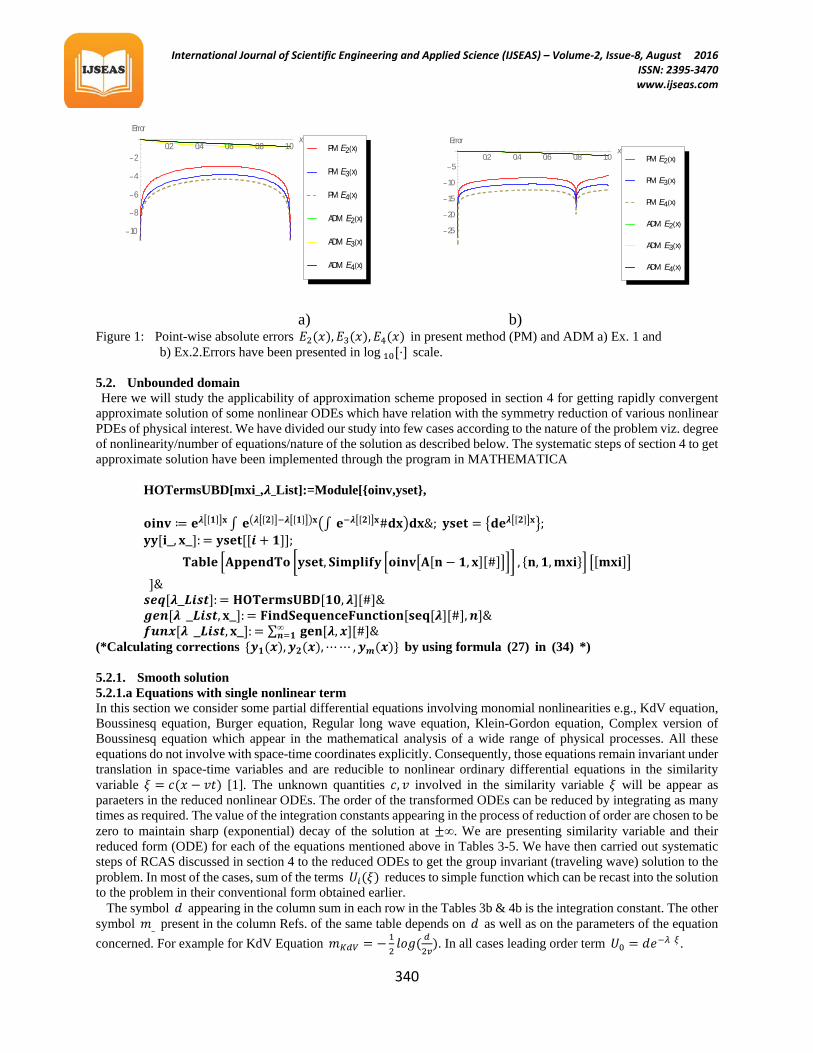
The Sup- and 𝐿2-errors of approximate solutions obtained by ADM and present method have been calculated and compared in Table 2. Their point-wise absolute errors have been graphically described in figure 1b. From the careful analysis of the results presented in Table 2 and Fig.1b it appears that approximate solutions obtained by present method for BVPs within bounded domain involving cubic nonlinearity are better than the results obtained by ADM. Table 2. Errors sup 𝐸𝑛 and 𝐿2𝐸𝑛 in ADM and present method of Ex. 2.

Error sup 𝐸1 𝐿2𝐸1 sup 𝐸2 𝐿2𝐸2 sup 𝐸3 𝐿2𝐸3 sup 𝐸4 𝐿2𝐸4

ADM .02 .01 .006 .004 .002 .001 .0009 .0006

PM .002 .001 .0002 .0002 .00003 .00002 4.9× 10−6 3.3 × 10−6


www.ijseas.com

340

a) b) Figure 1: Point-wise absolute errors 𝐸2(𝑥),𝐸3(𝑥),𝐸4(𝑥) in present method (PM) and ADM a) Ex. 1 and b) Ex.2.Errors have been presented in log 10[⋅] scale.

5.2. Unbounded domain Here we will study the applicability of approximation scheme proposed in section 4 for getting rapidly convergent approximate solution of some nonlinear ODEs which have relation with the symmetry reduction of various nonlinear PDEs of physical interest. We have divided our study into few cases according to the nature of the problem viz. degree of nonlinearity/number of equations/nature of the solution as described below. The systematic steps of section 4 to get approximate solution have been implemented through the program in MATHEMATICA

HOTermsUBD[mxi_,𝝀_List]:=Module[{oinv,yset}, 𝐨𝐢𝐧𝐯 ≔ 𝐞𝝀�[𝟏]�𝐱 ∫ 𝐞�𝝀�[𝟐]�−𝝀�[𝟏]��𝐱�∫ 𝐞−𝝀�[𝟐]�𝐱#𝐝𝐱�𝐝𝐱&; 𝐲𝐬𝐞𝐭 = �𝐝𝐞𝝀�[𝟐]�𝐱�; 𝐲𝐲[𝐢_, 𝐱_]: = 𝐲𝐬𝐞𝐭[[𝒊 + 𝟏]];

𝐓𝐚𝐛𝐥𝐞 �𝐀𝐩𝐩𝐞𝐧𝐝𝐓𝐨 �𝐲𝐬𝐞𝐭, 𝐒𝐢𝐦𝐩𝐥𝐢𝐟𝐲 �𝐨𝐢𝐧𝐯�𝐀[𝐧 − 𝟏, 𝐱][#]�� , {𝐧,𝟏,𝐦𝐱𝐢}� �[𝐦𝐱𝐢]� ]& 𝒔𝒆𝒒[𝝀_𝑳𝒊𝒔𝒕]: = 𝐇𝐎𝐓𝐞𝐫𝐦𝐬𝐔𝐁𝐃[𝟏𝟎,𝝀][#]& 𝒈𝒆𝒏[𝝀 _𝑳𝒊𝒔𝒕, 𝐱_]: = 𝐅𝐢𝐧𝐝𝐒𝐞𝐪𝐮𝐞𝐧𝐜𝐞𝐅𝐮𝐧𝐜𝐭𝐢𝐨𝐧[𝐬𝐞𝐪[𝝀][#],𝒏]& 𝒇𝒖𝒏𝒙[𝝀 _𝑳𝒊𝒔𝒕, 𝐱_]: = ∑ ∞

𝒏=𝟏 𝐠𝐞𝐧[𝝀,𝒙][#]& (*Calculating corrections {𝒚𝟏(𝒙),𝒚𝟐(𝒙),⋯⋯ ,𝒚𝒎(𝒙)} by using formula (27) in (34) *)

5.2.1. Smooth solution 5.2.1.a Equations with single nonlinear term In this section we consider some partial differential equations involving monomial nonlinearities e.g., KdV equation, Boussinesq equation, Burger equation, Regular long wave equation, Klein-Gordon equation, Complex version of Boussinesq equation which appear in the mathematical analysis of a wide range of physical processes. All these equations do not involve with space-time coordinates explicitly. Consequently, those equations remain invariant under translation in space-time variables and are reducible to nonlinear ordinary differential equations in the similarity variable 𝜉 = 𝑐(𝑥 − 𝑣𝑡) [1]. The unknown quantities 𝑐, 𝑣 involved in the similarity variable 𝜉 will be appear as paraeters in the reduced nonlinear ODEs. The order of the transformed ODEs can be reduced by integrating as many times as required. The value of the integration constants appearing in the process of reduction of order are chosen to be zero to maintain sharp (exponential) decay of the solution at ±∞. We are presenting similarity variable and their reduced form (ODE) for each of the equations mentioned above in Tables 3-5. We have then carried out systematic steps of RCAS discussed in section 4 to the reduced ODEs to get the group invariant (traveling wave) solution to the problem. In most of the cases, sum of the terms 𝑈𝑖(𝜉) reduces to simple function which can be recast into the solution to the problem in their conventional form obtained earlier. The symbol 𝑑 appearing in the column sum in each row in the Tables 3b & 4b is the integration constant. The other symbol 𝑚_ present in the column Refs. of the same table depends on 𝑑 as well as on the parameters of the equation concerned. For example for KdV Equation 𝑚𝐾𝑑𝑉 = −1

2𝑙𝑜𝑔( 𝑑

2𝑣). In all cases leading order term 𝑈0 = 𝑑𝑒−𝜆 𝜉.

0.2 0.4 0.6 0.8 1.0x

10

8

6

4

2

Error

ADM E4 x

ADM E3 x

ADM E2 x

PM E4 x

PM E3 x

PM E2 x0.2 0.4 0.6 0.8 1.0

x

25

20

15

10

5

Error

ADM E4 x

ADM E3 x

ADM E2 x

PM E4 x

PM E3 x

PM E2 x


www.ijseas.com

341

5.2.1.b System of equations In this section we consider some system of coupled PDEs e.g., generalised Zakharov, Devey-Stewartson, Klein-Gordon-Zakharov, coupled Higgs, Maccari equations which can be reduced to single ODE whenever field variables are expressed as the product of phase-amplitude factors and independent variables are expressed in terms of similarity variables as required by their symmetry transformations viz., space-time translations. Before solving those reduced ODEs by using method proposed here we first demonstrate the reduction of system of PDEs to ODEs with an example viz., Generalized Zakharov equation

𝑖𝐸𝑡 + 𝐸𝑥𝑥 + 2𝜆|𝐸|2𝐸 + 𝛿 𝜂𝐸 = 0 (55)

𝜂𝑡𝑡 − 𝑐2𝜂𝑥𝑥 + 𝜇(|𝐸|2)𝑥𝑥 = 0. (56) Transformations of field variables 𝐸(𝑥, 𝑡) to 𝐸(𝑥, 𝑡) = 𝑒𝑖(𝛼𝑥+𝛽𝑡)𝑢(𝜉), and 𝜂(𝑥, 𝑡) to 𝜂(𝑥, 𝑡) = 𝜂(𝜉), with similarity variables 𝜉 = 𝑘(𝑥 − 2𝛼𝑡) of above equations lead to the system of ODEs

𝑘2𝑢′′(𝜉) − (𝛼2 + 𝛽)𝑢(𝜉) + 𝛿𝑢(𝜉)𝜂(𝜉) + 2𝜆𝑢(𝜉)3 = 0, (57)

(4𝛼2 − 𝑐2)𝜂′′(𝜉) + 𝜇(𝑢(𝜉)2)′′ = 0. (58) One can now express the field variable 𝜂(𝜉) in terms of 𝑢(𝜉) by integrating (58) twice and taking integration constants to zero (assuming departure of 𝜂 from its equilibrium configuration at infinity is negligible) and get Table 3a: Similarity variables and reduction of some PDEs involving quadratic nonlinearity.

Eq. PDE 𝜉 Reduced ODE

KdV 𝑢𝑡 + 6𝑢𝑢𝑥 + 𝑢𝑥𝑥𝑥 = 0 𝑐(𝑥 − 𝑣𝑡) 𝑢′′ −𝑣𝑐2𝑢 +

3𝑐2𝑢2 = 0

Boussinesq(B) 𝑢𝑡𝑡 + 𝑎𝑢𝑥𝑥 + 𝑏(𝑢2)𝑥𝑥 + 𝑐𝑢𝑥𝑥𝑥𝑥 = 0 𝑘(𝑥 − 𝑣𝑡) 𝑢′′ − (𝑎𝑣2

−𝑐𝑘2)𝑢 +

𝑏𝑐𝑘2

𝑢2 = 0

RLW 𝑢𝑡 + 𝑢𝑥 + 𝑎𝑢𝑢𝑥 − 𝑏𝑢𝑥𝑥𝑡 = 0 𝑐(𝑥 − 𝑣𝑡) 𝑢′′ − ((𝑣 − 1)𝑐2𝑏𝑣

)𝑢 +𝑎

2𝑏𝑣𝑐2𝑢2 = 0

Klein-Gordon(KG) 𝑢𝑡𝑡 − 𝛼2𝑢𝑥𝑥 + 𝛽𝑢 − 𝛾𝑢2 = 0 𝑘(𝑥 − 𝑐𝑡) 𝑢′′ −𝛽

𝑘2(𝛼2 − 𝑐2)𝑢 −

𝛾𝑘2(𝛼2 − 𝑐2)

𝑢2 = 0

Complex Boussinesq(CB) 𝑢𝑡𝑡 − 𝛾𝑢𝑥𝑥 − 𝛼𝑢𝑥𝑥𝑥𝑥 − 𝛽(𝑢2)𝑥𝑥 = 0 𝑖𝑘(𝑥 − 𝑐𝑡) 𝑢′′ − (

𝛾 − 𝑐2

𝛼𝑘2)𝑢 −

𝛽𝛼 𝑘2

𝑢2 = 0

Zakharov- Kuznetsov(ZK) 𝑢𝑡 + 𝛿𝑢𝑥 + 𝛼𝑢𝑢𝑥 + 𝛽𝑢𝑥𝑥𝑥 + 𝛾𝑢𝑥𝑥𝑦 = 0 𝑘𝑥 + 𝑙𝑦 − 𝑐𝑡 𝑢′′ − (𝑐−𝛿𝑘)

(𝛽𝑘3+𝛾𝑘2𝑙)+ 𝛼𝑘

2(𝛽𝑘3+𝛾𝑘2𝑙)𝑢2 = 0

Kadomtsev- Petviashvili(KP) (𝑢𝑡 + 6𝑢𝑢𝑥 + 𝑢𝑥𝑥𝑥)𝑥 + 3𝑢𝑦𝑦 + 3𝑢𝑧𝑧 = 0 𝑎𝑥 + 𝑏𝑦 + 𝑐𝑧 − 𝛿𝑡 𝑢′′ +

(3𝑏2 + 3𝑐2 − 𝑎𝛿)𝑎4

𝑢 +3𝑎2𝑢2 = 0

Table 3b: Leading order and correction terms of the Approx. Soln. In (29) and their sum.

Eq. 𝜆 𝑈0 𝑈𝑛 sum Refs.

KdV √𝑣𝑐

𝑑𝑒−𝜆 𝜉

−21−𝑛𝑛𝑣 �−𝛿𝑒−𝜆 𝜉

𝑣�𝑛

4𝑒𝜆 𝜉𝑣2𝑑(2𝑒𝜆 𝜉𝑣 + 𝑑)2

𝑣2𝑆𝑒𝑐ℎ2(

12𝜆 𝜉 + 𝑚𝐾𝑑𝑉)

[5]


www.ijseas.com

342

B �−𝑎 + 𝑣2

𝑐𝑘2


61−𝑛𝑛(𝑎 + 𝑣2) �𝑏𝑑𝑒−𝜆 𝜉

𝑎 + 𝑣2 �𝑛

𝑏

36𝑑(𝑎 + 𝑣2)2𝑒𝜆 𝜉

(6𝑣2𝑒𝜆 𝜉 + 6𝑎𝑒𝜆 𝜉 − 𝑏𝑑)2

−3(𝑎 + 𝑣2)

2𝑏sech2 �

12𝜆 𝜉 + 𝑚𝐵𝑜𝑢�

[22]

RLW �𝑣 − 1𝑏𝑐2𝑣


−12𝑛(𝑣 − 1)

𝑎�𝑎𝑑𝑒−𝜆 𝜉

12 − 12𝑣�𝑛

144𝑑(𝑣 − 1)2𝑒𝜆 𝜉

(𝑎𝑑 − 12𝑒𝜆 𝜉 + 12𝑣𝑒𝜆 𝜉)2

3(𝑣 − 1)𝑎

sech2(𝜆2𝜉 + 𝑚𝑅𝐿𝑊)

[23]

KG �𝛽

𝑘2(𝛼2 − 𝑐2)


−61−𝑛𝑛𝛽

𝛾�−

𝑑𝛾𝛽𝑒−𝜆 𝜉�

𝑛

36𝑑𝛽2𝑒𝜆 𝜉

(6𝛽𝑒𝜆 𝜉 + 𝑑𝛾)2

3(𝑣 − 1)𝑎

sech2 �𝜆2𝜉 + 𝑚𝐾𝐺�

[24]

CB �𝛾 − 𝑐2

𝑘2𝛼


−6𝑛(𝑐2 − 𝛾)

𝛽�−

𝑑𝛽𝑒−𝜆 𝜉

6𝑐2 − 6𝛾�𝑛

36𝑑(𝑐2 − 𝛾)2𝑒𝜆 𝜉

(6𝑐2𝑒𝜆 𝜉 − 6𝛾𝑒𝜆 𝜉 + 𝑑𝛽)2

3(𝑐2 − 𝛾)2𝛽

𝑠𝑒𝑐ℎ2(𝑖𝜆𝜉2

+ 𝑚𝐶𝐵)

[25]

ZK �𝑐 − 𝑘𝛿

𝑘3𝛽 + 𝑘2𝑙𝛾


121−𝑛𝑛(𝑘𝛿 − 𝑐)𝑘𝛼

�𝑑𝑘𝛼𝑒−𝜆 𝜉

𝑘𝛿 − 𝑐�𝑛

144𝑑(𝑐 − 𝑘𝛿)2𝑒𝜆 𝜉

(12𝑐𝑒𝜆 𝜉 − 12𝑘𝛿𝑒𝜆 𝜉 + 𝑑𝑘𝛼)2

3(𝑐 − 𝑘𝛿)𝑘𝛼

𝑠𝑒𝑐ℎ2(𝜆2𝜉 + 𝑚𝑍𝐾)

[26]

KP �(3𝑏2 + 3𝑐2 − 𝑎𝛿)−𝑎4


−2𝑛(𝑎𝛿 − 3b2 − 3𝑐2)�𝑎2𝑑𝑒−𝜆𝜉�𝑛

𝑎2(−2𝑎𝛿 + 6b2 + 6𝑐2)𝑛

4𝑑(−𝑎𝛿 + 3b2 + 3𝑐2)2𝑒𝜆 𝜉

((−2𝑎𝛿 + 6b2 + 6𝑐2)𝑒𝜆 𝜉 − 𝑎2𝑑)2

(𝑎𝛿 − 3𝑏2 − 3𝑐2)2𝑎2

𝑠𝑒𝑐ℎ2(𝜆 𝜉2

+ 𝑚𝑍𝑃)

[27]

𝜂(𝜉) = 𝜇

(𝑐2−4𝛼2)𝑢(𝜉)2, 𝑐2 ≠ 4𝛼2. (59)

Now Eqs. (57) and (58) can be decoupled by using (59) into (57) to get equation for 𝑢(𝜉) as 𝑢′′(𝜉) − (𝛼2+𝛽)

𝑘2𝑢(𝜉) − (𝛿𝜇−2𝜆(4𝛼2−𝑐2))

𝑘2(4𝛼2−𝑐2)𝑢(𝜉)3 = 0. (60)

This equation is suitable for the application of RCAS developed in section 4 to obtain approximate or exact solution to the problem. Substitution of that solution into (59) provides approximate/exact solution of 𝜂(𝜉). Further substitution of expression for 𝜉 into those formula will give space-time dependent solution of the Generalized Zakharov system of equations. Following similar procedure one can find solutions of other such systems of equations summarized in Table 6a & 6b.

5.2.2 Non smooth solution In 1993, Camassa and Holm [40, 41] derived an equation

𝑣𝑡 + 2𝑘𝑣𝑥 − 𝑣𝑥𝑥𝑡 + 3𝑣𝑣𝑥 − 2𝑣𝑥𝑣𝑥𝑥 − 𝑣𝑣𝑥𝑥𝑥 = 0 (61) for shallow water wave with 𝑣(𝑥, 𝑡) related to a layer-mean horizontal velocity at the spatial coordinate 𝑥 and time 𝑡. This equation now known as Camassa−Holm (CH) equation was derived as an asymptotic model for long gravity waves at the surface of shallow water. Because the dispersive term is nonlinear this equation has peaked solitary wave solutions of the form

𝑣(𝑥, 𝑡) = 𝑐𝑒−|𝑥−𝑐𝑡| (62) for 𝑘 = 0, which travels with wave speed 𝑐. The solitary wave solution (62) known as peakon, has a distinct feature like discontinuous first derivative at the wave peak in contrast to smoothness of conventional solitary waves. However, we have applied RCAS proposed here to the ODE associated to the CH equation for 𝑘 ≠ 0 and obtained peakon solution as given in the Table 7a,b.

A snap of the wave at some instant is given by the function 𝑣(𝑥, 𝑡) is displayed in Fig.2 for 𝑑 = 15 and 𝑘 = .001. From last expression it appears that although the traveling wave solution 𝑣(𝑥, 𝑡) of CH equation maintains soliton-like behaviour throughout the motion continuous at 𝑥 = 𝑐𝑡, its derivative is not continuous there. As a result the solution maintains a sharp peak at 𝑥 = 𝑐𝑡 throughout the motion. Table 4a: Similarity variables and reduced ODEs of some PDEs involving cubic nonlinearity.

Eq. PDE Transformation Reduced ODE


www.ijseas.com

343

Dispersive(Dis) 𝑢𝑡 − 𝛿 𝑢2𝑢𝑥 + 𝑢𝑥𝑥𝑥 = 0 𝜉 = 𝑘(𝑥 − 𝜆 𝑡) 𝑢′′ −𝜆𝑘2𝑢 −

𝛿3 𝑘2

𝑢3 = 0

𝜙4 𝑢𝑡𝑡 − 𝛼𝑢𝑥𝑥 − 𝑢 + 𝑢3 = 0 𝜉 = 𝑐(𝑥 − 𝑣 𝑡) 𝑢′′ −1

𝑐2(𝑣2 − 𝛼)𝑢 +

1𝑐2(𝑣2 − 𝛼)

𝑢3 = 0

Cubic Klein- Gordon(CKG) 𝑢𝑡𝑡 − 𝛼2𝑢𝑥𝑥 + 𝛽𝑢 − 𝛾𝑢3 = 0 𝜉 = 𝑘(𝑥 − 𝑐 𝑡) 𝑢′′ −

𝛽𝑘2(𝛼2 − 𝑐2)

𝑢 −𝛾

𝑘2(𝛼2 − 𝑐2)𝑢3 = 0

The generalised ZK-BBM(GZK)

𝑢𝑡 + 𝑢𝑥 + 𝑎(𝑢3)𝑥 + 𝑏(𝑢𝑥𝑡 + 𝑢𝑦𝑦)𝑥 = 0

𝜉 = 𝑟𝑡 + 𝑝𝑥 + 𝑞𝑦

𝑢′′ +(𝑝 + 𝑟)

𝑏𝑝(𝑞2 + 𝑝𝑟)𝑢 +

𝑎𝑏(𝑞2 + 𝑝𝑟)

𝑢3 = 0

Schr�̈�dinger(Sch) 𝑖𝐸𝑡 + 𝐸𝑥𝑥 − 𝜇|𝐸|2𝐸 = 0 𝐸 = 𝑒𝑖(𝛼𝑥+𝛾𝑡)𝑢(𝜉) , 𝜉 = 𝑘(𝑥 − 2𝑐𝑡)

𝑢′′ − (𝛾 − 𝛼2

𝑘2)𝑢 +

𝜇𝑘2𝑢3 = 0

Hamiltonian Amplitude(HA) 𝑖𝐸𝑥 + 𝐸𝑡𝑡 + 2𝜎|𝐸2|𝐸 − 𝜀𝐸𝑥𝑡 = 0

𝐸 = 𝑒𝑖(𝛼𝑥−𝛽𝑡)𝑢(𝜉) 𝜉 = (2𝛽 + 𝛼𝜀)𝑥

+(1 + 𝛽𝜀)𝑡

𝑢′′ −(𝛽2 + (1 + 𝛽𝜀)𝛼)

(1 − 𝛽2𝜀2 − (𝜀2 + 𝛽𝜀3)𝛼)𝑢

=2𝜎

((𝜀2 + 𝛽𝜀3) + 𝛽2𝜀2 − 1)𝑢3

Table 4b: Leading order and correction terms of (29) and their sum. Eq. 𝜆 𝑈0 𝑈𝑛 sum Refs.

Dis. √𝜆𝑘


241−𝑛𝜆𝑒−𝜆 𝜉

𝑑𝛿�𝑑

2𝛿𝑒−2𝜆 𝜉

𝜆�𝑛

24𝑑𝜆𝑒𝜆 𝜉

24𝜆𝑒2𝜆 𝜉−𝑑2𝛿

�−6𝜆

𝛿 sech(𝜆𝜉 + 𝑚𝐷𝑖𝑠)

[28]

𝜙4 � 1

𝑐2(𝑣2−𝛼)

𝑑𝑒−𝜆 𝜉 −81−𝑛𝑒𝜆 𝜉�−𝑑2𝑒−2𝜆 𝜉�

𝑛

𝑑

8𝑑𝑒𝜆 𝜉

8𝑒2𝜆 𝜉+𝑑2

√2 sech(𝜆 𝜉 + 𝑚Φ) [29]

CKG � 𝛽𝑘2(𝛼2−𝑐2)


−81−𝑛𝛽𝑒𝜆 𝜉

𝑑𝛾�− 𝑑2𝛾𝑒−2𝜆 𝜉

𝛽�𝑛

8𝑑𝛽𝑒𝜆 𝜉

8𝛽𝑒2𝜆 𝜉+𝑑2𝛾

�2𝛽

𝛾 sech(𝜆 𝜉 + 𝑚𝐶𝐾𝐺)

[24]

GZK �−

𝑝+𝑟𝑏𝑝(𝑝𝑟+𝑞2)


81−𝑛(𝑝+𝑟)𝑒𝜆 𝜉

𝑎𝑑𝑝�𝑎𝑑

2𝑝𝑒−2𝜆 𝜉

𝑝+𝑟�𝑛

8𝑑(𝑝+𝑟)𝑒𝜆 𝜉

−𝑎𝑑2𝑝+8𝑝𝑒2𝜆 𝜉+8𝑟𝑒2𝜆 𝜉

�−2(𝑝+𝑟)

𝑎𝑝 sech(𝜆 𝜉 + 𝑚𝐺𝑍𝐾)

[30]

Sch. �𝛼2+𝛾𝑘


−81−𝑛�𝛼2+𝛾�𝑒𝜆 𝜉

𝑑𝜇�− 𝑑2𝜇𝑒−2𝜆 𝜉

𝛼2+𝛾�𝑛

8𝑑�𝛼2+𝛾�𝑒𝜆 𝜉

𝑑2𝜇+8𝛼2𝑒2𝜆 𝜉+8𝛾𝑒2𝜆 𝜉

�2(𝛼2+𝛾)

𝜇 sech(𝜆 𝜉 + 𝑚𝑆𝑐ℎ)

[31]


www.ijseas.com

344

HA � 𝛼(𝛽𝜀+1)+𝛽2

1−𝛼(𝛽𝜀3+𝜀2)−𝛽2𝜀2

𝑑𝑒−𝜆 𝜉 −41−𝑛�−𝑑2𝜎𝑒−2𝜆 𝜉�

𝑛𝑒−𝜆 𝜉

𝑑𝜎(𝛼𝛽𝜀+𝛼+𝛽2)𝑛−1

4𝑑�𝛼𝛽𝜀+𝛼+𝛽2�𝑒𝜆 𝜉

𝑑2𝜎+(4𝛽2+4𝛼+4𝛼𝛽𝜀)𝑒2𝜆 𝜉

�𝛼𝛽𝜀+𝛼+𝛽2

𝜎 sech(𝜆 𝜉 + 𝑚𝐻𝐴)

[30]

Table 5a: Similarity reduction of PDEs involving biquadratic nonlinearities.

Eq. PDEs Transformation Reduced ODE

gKdV 𝑢𝑡 + 𝛿 𝑢𝑥𝑥𝑥 + 𝑢3𝑢𝑥 = 0 𝜉 = 𝑐(𝑥 − 𝑣𝑡) 𝑢′′ − 𝑣𝛿𝑐2

𝑢 + 𝑎4𝛿𝑐2

𝑢4 = 0

Table 5b: Leading and general term of the series in (29) and their sum for reduced ODE ( (a)n → Pochhammer symbol).

Eq. 𝜆 𝑈𝑛 sum Refs.

gKdV �𝑣𝛿𝑐2

−

401−𝑛𝑣𝑒2𝜆 𝜉 �−𝑎𝑑3𝑒−3𝜆 𝜉

𝑣 �𝑛

𝑎𝑑2×

(23)

n−1(1)n−1

4𝑑𝜆𝑒−𝜆 𝜉

�8 + 𝑎𝑑35𝑣 𝑒−3𝜆 𝜉�

23

(10𝑣𝑎

)13𝑠𝑒𝑐ℎ

23(32𝜆𝜉 + 𝑚) [32]

Table 6a: Similarity reduction of system of PDEs involving cubic nonlinearities.


Generalised Zakharov(GZ)

𝑖𝐸𝑡 + 𝐸𝑥𝑥 + 2𝜆|𝐸|2𝐸 + 𝛿 𝜂𝐸 = 0 𝜂𝑡𝑡 − 𝑐2𝜂𝑥𝑥 + 𝜇(|𝐸|2)𝑥𝑥 = 0

𝐸 = 𝑒𝑖(𝛼𝑥+𝛽𝑡)𝑢(𝜉) 𝜂 = 𝜂(𝜉)

𝜉 = 𝑘(𝑥 − 2𝛼𝑡)

𝑢′′ − (𝛼2+𝛽)𝑘2

𝑢 − (𝛿𝜇−2𝜆(4𝛼2−𝑐2))𝑘2(4𝛼2−𝑐2)

𝑢3 = 0

Devey- Stewartson(DS)

𝑖𝐸𝑡 + 𝐸𝑥𝑥 − 𝐸𝑦𝑦 − 2|𝐸|2𝐸 − 2𝐸𝜂 = 0 𝜂𝑥𝑥 + 𝜂𝑥𝑥 + 2(|𝐸|2)𝑥𝑥 = 0

𝐸 = 𝑒𝑖(𝑝𝑥+𝑞𝑦+𝑟𝑡)𝑢(𝜉) 𝜂 = 𝜂(𝜉)

𝜉 = 𝑘𝑥 + 𝑐𝑦 + 2(𝑐𝑞 − 𝑘𝑝)𝑡

𝑢′′ + (𝑞2−𝑝2−𝑟)(𝑘2−𝑐2)

𝑢 + 2(𝑘2+𝑐2)

𝑢3 = 0

Klein-Gordon- Zakharov(KGZ)

𝐸𝑡𝑡 − 𝐸𝑥𝑥 + 𝐸 − 𝛼𝜂𝐸 = 0 𝜂𝑡𝑡 − 𝜂𝑥𝑥 − 𝛽(|𝑢|2)𝑥𝑥 = 0

𝐸 = 𝑒𝑖(𝑘𝑥+𝑤𝑡)𝑢(𝜉) 𝜂 = 𝜂(𝜉)

𝜉 = 𝑤𝑥 + 𝑘𝑡

𝑢′′ − (𝑤2−𝑘2−1)(𝑘2−𝑤2)

𝑢 − 𝛼𝛽𝑤2

(𝑘2−𝑤2)2𝑢3 = 0


www.ijseas.com

345

Coupled Higgs(CHs)

𝑢𝑡 − 𝑢𝑥𝑥 + |𝑢|2𝑢 − 2𝜂𝑢 = 0 𝜂𝑡𝑡 + 𝜂𝑥𝑥 − (|𝑢|2)𝑥𝑥 = 0

𝐸 = 𝑒𝑖(𝑝𝑥+𝑟𝑡)𝑢(𝜉) 𝜂 = 𝜂(𝜉) 𝜉 = 𝑟𝑥 + 𝑝𝑡

𝑢′′ + 𝑢 + 𝑢3

(𝑝2+𝑟2)= 0

Maccari systems(Mc)

𝑖𝐸𝑡 + 𝐸𝑥𝑥 + 𝜂𝐸 = 0 𝜂𝑡 + 𝜂𝑦 − (|𝐸|2)𝑥

𝐸 = 𝑒𝑖(𝑝𝑥+𝑞𝑦+𝑟𝑡)𝑢(𝜉) 𝜂 = 𝜂(𝜉)

𝜉 = 𝑘(𝑥 − 2𝑝𝑡) + 𝑞𝑦

𝑢′′ − 1𝑘2

(𝑝2 + 𝑟 − 𝑐𝑞−2𝑘𝑝

)𝑢 − 𝑢3

𝑘(𝑞−2𝑘𝑝)= 0

Figure 2: Peakon Soln. Of CH Eq. Obtained by present method.

Table 6b: Leading and correction terms in (29) and their sum.

Eq. 𝜆 𝑈𝑛 sum Refs. GZ �𝛼

2+𝛽𝑘

−81−𝑛(4𝛼2−𝑐2)(𝛼2+𝛽)𝑒𝜆𝜉

𝑑(−2𝑐2𝜆1+8𝛼2𝜆1−𝛿𝜇) ×

�−𝑑2𝑒−𝜆𝜉(2𝑐2𝜆1−8𝛼2𝜆1+𝛿𝜇)

(𝑐2−4𝛼2)(𝛼2+𝛽) �𝑛

𝑑𝜆𝑒−𝜆 𝜉

1+𝑑2(2𝑐2𝜆−8𝛼2𝜆+𝛿𝜇)8(𝑐2−4𝛼2)(𝛼2+𝛽) 𝑒

−2𝜆 𝜉

�2(𝑐2−4𝛼2)(𝛼2+𝛽)(2𝑐2𝜆−8𝛼2𝜆+𝛿𝜇)

×

sech(𝜆𝜉 + 𝑚𝐺𝑍) [33, 34]

DS �(𝑝2−𝑞2+𝑟)

(𝑘2−𝑐2)

41−𝑛(𝑐2 + 𝑘2)(𝑝2 − 𝑞2 + 𝑟)𝑒𝜆 𝜉

𝑑(𝑐2 − 𝑘2) ×

�𝑑(𝑐2 − 𝑘2)𝑒−2𝜆 𝜉

(𝑐2 + 𝑘2)(𝑝2 − 𝑞2 + 𝑟)�𝑛

𝑑𝑒−𝜆𝜉

1− 𝑑2�𝑐2−𝑘2�𝑒−2𝜆𝜉

4�𝑐2+𝑘2��𝑝2−𝑞2+𝑟�

−2𝑘2(𝑝2−𝑞2+𝑟)(𝑐2−𝑘2)

×

sech(𝜆 𝜉 + 𝑚𝐷𝑆) [35, 36]

4 2 2 4

5

10

15

Solution


www.ijseas.com

346

KGZ �(𝑤2−𝑘2−1)

(𝑘2−𝑤2)

81−𝑛(𝑘4−2𝑘2𝑤2+𝑘2+𝑤4−𝑤2)𝑒𝜆𝜉

𝑑𝑤2𝛼𝛽×

� 𝑑2𝑤2𝛼𝛽𝑒−2𝜆𝜉

𝑘4−2𝑘2𝑤2+𝑘2+𝑤4−𝑤2�𝑛

𝑑𝑒𝜆 𝜉

1− 𝑑2𝑤2𝛼 𝛽𝑒2𝜆 𝜉

8(𝑘2+𝑘4−𝑤2−2𝑤2𝑘2+𝑤4)

�2(𝑤2−𝑘2−𝑘4+2𝑤2𝑘2−𝑤4)𝛼𝛽𝑤

×

sech(𝜆 𝜉 + 𝑚𝐾𝐺𝑍) [37]

CHs 𝑖

81−𝑛(𝑝2+𝑟2)𝑒𝜆 𝜉

𝑑×

�𝑑2𝑒−2𝜆 𝜉

𝑝2 + 𝑟2 �𝑛


1− 𝑒−2𝜆 𝜉

8(𝑝2+𝑟2)

�−2(𝑝2 + 𝑟2) × sech(𝜆𝜉 + 𝑚𝐶𝐻)

[38, 39]

Mc �

(𝑝2+𝑟− 𝑐𝑞−2𝑘𝑝)

𝑘2

−81−𝑛𝑒𝜆𝜉(𝑐+2𝑘𝑝3+2𝑘𝑝𝑟−𝑝2𝑞−𝑞𝑟)𝑑𝑘

×

�− 𝑑2𝑘𝑒−2𝜆𝜉

𝑐+(𝑝2+𝑟)(2𝑘𝑝−𝑞)�𝑛


1+ 𝑑2𝑘𝑒−2𝜆 𝜉

8�𝑐+2𝑘𝑝3+2𝑘𝑝𝑟−𝑝2𝑞−𝑞𝑟�

�2(𝑐+2𝑘𝑝3+2𝑘𝑝𝑟−𝑝2𝑞−𝑞𝑟)𝑘

×

sech(𝜆 𝜉 + 𝑚𝑀𝑐) [38, 39]

Table 7a: Similarity reduction of CH Eq.


Camassa- Holm

𝑣𝑡 + 2𝑘𝑣𝑥 − 𝑣𝑥𝑥𝑡 + 3𝑣𝑣𝑥 −2𝑣𝑥𝑣𝑥𝑥 − 𝑣𝑣𝑥𝑥𝑥 = 0

𝑣(𝑥, 𝑡) = 𝑢(𝜉) − 𝑘 𝜉 = 𝑥 − 𝑐𝑡

𝑢′′ − 𝑢 − 12(𝑘+𝑐)

(𝑢′2 + 2𝑢𝑢′′ − 3𝑢2) = 0

Table 7b: Leading order and correction terms of series in (29) and their sum.

Condition 𝜆 𝑈0 𝑈1 𝑈𝑛 sum Soln. 𝑣(𝑥, 𝑡) in [42]

when 𝑥 − 𝑐 𝑡 ≻ 0

𝑤ℎ𝑒𝑛 𝑥 − 𝑐 𝑡 ≺ 0

1

1

𝑑𝑒−𝜆𝜉

𝑑𝑒𝜆𝜉

0

0

0

0

𝑑𝑒−𝜆𝜉

𝑑𝑒𝜆𝜉

𝑑 𝑒−(𝑥−𝑐𝑡) − 𝑘

𝑑 𝑒+(𝑥−𝑐𝑡) − 𝑘

6 Conclusion This work deals with an approximation scheme to obtaining a rapidly convergent approximate solution of nonlinear ODEs with DBCs defined over bounded/ unbounded domain. An advantage of the present method is that the boundary condition at ±∞ ( BVP in unbounded domain ) can be incorporated into the solution in a natural way rather than taking recourse to the use of Padé approximant of the higher order corrections terms as desired in case of ADM. From the theory developed here and case studies presented we have arrived at the following conclusion. 1. When the linear part of the nonlinear equation involves only the highest derivative (𝜆1 = 𝜆2 = 0), the inverse operator of the RCAS became identical with that of the ADM. In that case the algorithms of the proposed scheme coincide with those of ADM. 2. For 𝜆1 ≠ 𝜆2 ≠ 0 , the the proposed schemes for both bounded and unbounded domains provide a rapidly convergent series solution (𝑆1) in comparision to the same (𝑆2) found by using ADM. More significantly, partial sum of terms in 𝑆1 is more accurate result than the corresponding sum of terms in 𝑆2. As a result, one can use the present scheme to obtain exact solutions in localized within finite space of nonlinear differential equations. 3. The algorithm presented here can evaluate successive correction terms more efficiently in comparison to ADM not only for the two-point boundary value problems but are also equally effective for solving initial-boundary value problems involving PDEs exhibiting translational symmetry in both space and time variables. 4. The formulae for successive correction terms presented here can be easily implemented through the symbolic computation software viz. Mathematica, Maple, Matlab etc. The programmes in MATHEMATICA for calculating Adomian polynomials, successive correction terms and their general form, getting sum of the series have been presented here for their use. 5. The travelling wave solutions of several nonlinear scalar or system of coupled PDEs appearing in the mathematical analysis of varieties of physical processes have been obtained by using RCAS developed here and summarized in the


www.ijseas.com

347

tables for their easy access. We conclude by noting that it remains an interesting curiosity to treat the initial boundary value problems modeled by partial differential equations involving variable coefficients which apparently do not exhibit space-time translational symmetry. In this context we note that very often one can look for change of dependent and independent variables to convert the partial differential equations with variable coefficients to similar equations with constant coefficient and thereby regain the appropriate symmetry. Works in these directions are in progress and will be reported in due course.

Acknowledgement This work is supported by UGC assisted SAP(DRS Phase-II) program grant No. F.510/4/DRS/2009(SAP-I) through Department of Mathematics, Visva-Bharati, Santiniketan-731 235, W.B., India References [1] P. J. Olver, Applications of Lie groups to differential equations, Vol. 107, Springer Science & Business Media, 2000. [2] N. H. Ibragimov, CRC Handbook of Lie group analysis of differential equations, Vol. 1,2,3, CRC press, 1994, 1994, 1996. [3] A. G. Choudhury, P. Guha, and B. Khanra, ''Solutions of some second order odes by the extended prelle-singermethod and symmetries'', J. Nonlin. Math. Phys., Vol. 15, No. 4, 2008, pp. 365–382. [4] M. Nucci, and P. Leach, ''Jacobis last multiplier and the complete symmetry group of the ermakov-pinney equation'', J. Nonlin. Math. Phys., Vol. 12, No. 2, 2005, pp. 305–320. [5] W. Malfliet, ''Solitary wave solutions of nonlinear wave equations'', Am. J. Phys., Vol. 60, No. 7, 1992, pp. 650–654. [6] W. Malfliet, and W. Hereman, ''The tanh method:1 exact solutions of nonlinear evolution and wave equations'', Phys. Scr., Vol. 54, 1996, pp. 563–568. [7] S. Abbasbandy, E. Magyari, and E. Shivanian, ''The homotopy analysis method for multiple solutions of nonlinear boundary value problems'', Comm. Nonlin. Sc. Num. Simul., Vol. 14, No. 9, 2009, pp. 3530–3536. [8] S. Xinhui, Z. Liancun, Z. Xinxin, and S. Xinyi, ''Homotopy analysis method for the asymmetric laminar flow and heat transfer of viscous fluid between contracting rotating disks'', Appl. Math. Model., Vol. 36, No. 4, 2012, pp. 1806–1820. [9] G. Adomian, Solving frontier problems of physics: the decomposition method: The Decomposition Method Kluwer, 1994. [10] J.-S. Duan and R. Rach, ''A new modification of the adomian decomposition method for solving boundary value problems for higher order nonlinear differential equations'', Appl. Math. Comput., Vol. 218, No. 8, 2011, pp. 4090–4118. [11] G. Adomian, and R. Rach,'' Inversion of nonlinear stochastic operators'', J. Math. Anal. Appl., Vol. 91, No. 1, 1983, pp. 39–46. [12] G. Adomian, and R. Rach, ''Analytic solution of nonlinear boundary-value problems in several dimensions by decomposition'', J. Math. Anal. Appl., Vol. 174 No. 1, 1993, pp. 118–137. [13] G. Adomian, and R. Rach, ''A new algorithm for matching boundary conditions in decomposition solutions'', Appl. math. comput., Vol. 57 , No. 1, 1993, pp. 61–68. [14] G. Adomian, and R. Rach, ''Modified decomposition solution of linear and nonlinear boundary-value problems'', Nonlin. Anal. Th. Meth. Appl., Vol. 23, No. 5, 1994, pp. 615–619. [15] A.-M. Wazwaz, ''Approximate solutions to boundary value problems of higher order by the modified decomposition method'', Comput. Math. Appl., Vol. 40, No. 6, 2000, pp. 679–691. [16] A.-M. Wazwaz, ''The modified adomian decomposition method for solving linear and nonlinear boundary value problems of tenth-order and twelfth-order'', Int. J. Nonlin. Sci. Num. Simul., Vol. 1, No. 1, 2000, pp. 17–24. [17] A. Wazwaz, ''A reliable algorithm for obtaining positive solutions for nonlinear boundary value problems'', Comput. Math. Appl., Vol. 41, No. 10, 2001, pp. 1237–1244. [18] A.-M. Wazwaz, ''The numerical solution of fifth-order boundary value problems by the decomposition method'', J. Comput. Appl. Math., Vol. 136 , No. 1, 2001, pp. 259–270. [19] A.-M.Wazwaz, ''The numerical solution of sixth-order boundary value problems by the modified decomposition method'', Appl. Math. Comput., Vol. 118 , No. 2, 2001, pp. 311–325.


www.ijseas.com

348

[20] A.-M. Wazwaz, ''A reliable algorithm for solving boundary value problems for higher-order integro-differential equations'', Appl. Math. Comput., Vol. 118, No. 2, 2001, pp. 327–342. [21] A.-M. Wazwaz, ''The numerical solution of special fourth-order boundary value problems by the modified decomposition method'', Int. J. comput. math., Vol. 79, No. 3, 2002, pp. 345–356. [22] P. A. Clarkson, and M. D. Kruskal,'' New similarity reductions of the boussinesq equation'', J. Math. Phys., Vol. 30, No. 10, 1989, pp. 2201–2213. [23] T. S. El-Danaf, M. A. Ramadan, and F. E. A. Alaal, ''The use of adomian decomposition method for solving the regularized long-wave equation'', Chaos, Solitons & Fractals, Vol. 26, No. 3, 2005, pp. 747–757. [24] H. Zhang, ''New exact travelling wave solutions for some nonlinear evolution equations, part ii'', Chaos, Solitons & Fractals, Vol. 37, No. 5, 2008, pp. 1328–1334. [25] H. Zhang, ''A new sub-equation method applied to obtain exact travelling wave solutions of some complex nonlinear equations'', Chaos, Solitons & Fractals, Vol. 42, No. 2, 2009, pp. 911–915. [26] J.-H. He, ''Application of homotopy perturbationmethod to nonlinear wave equations'', Chaos, Solitons & Fractals, Vol. 26, No. 3, 2005, pp. 695–700. [27] M. A. Akbar, N. Hj, M. Ali, and S. T. Mohyud-din, ''Some new exact traveling wave solutions to the (3+ 1)-dimensional kadomtsev-petviashvili equation'', World Appl. Sci. J, Citeseer, 2012. [28] A. J. Mohamad-Jawad, ''The sine-cosine function method for exact solutions of nonlinear partial differential equations'', IJRRS, Vol. 13, No. 1. [29] M. Younis, and A. Zafar, ''The modified simple equation method for solving nonlinear phi-four equation'', Inter. J. Innovation and Applied Studies , Vol. 2, No. 4, 2013, pp. 661–664. [30] M. Abdou, ''The extended f-expansion method and its application for a class of nonlinear evolution equations'', Chaos, Solitons & Fractals, Vol. 31, No. 1, 2007, pp. 95–104. [31] W.-X. Ma, and M. Chen, ''Direct search for exact solutions to the nonlinear schrodinger equation'', Appl. Math. Comput., Vol. 215, No. 8, 2009, pp. 2835–2842. [32] W. Hereman, and M. Takaoka, ''Solitary wave solutions of nonlinear evolution and wave equations using a direct method and macsyma'', J. Phys. A: Mathematical and General, Vol. 23, No. 21, 1990, pp. 4805. [33] V. E. Zakharov, ''Collapse of langmuir waves'', Soviet Journal of Experimental and Theoretical Physics, Vol. 35, 1972, pp. 908. [34] W.-H. Steeb, N. Euler, and W. Hereman,'' A note on the zakharov equation and lie-symmetry vector fields'', Il Nuovo Cimento B, Vol. 107 , No. 10, 1992, pp. 1211–1213. [35] M. Abdou, ''The extended tanh method and its applications for solving nonlinear physical models'', Appl. Math. Comput., Vol. 190, No. 1, 2007, pp. 988–996. [36] S. El-Wakil, M. Abdou, and A. Elhanbaly, '' New solitons and periodic wave solutions for nonlinear evolution equations'', Phys. Lett. A, Vol. 353, No. 1, 2006, pp. 40–47. [37] Y. Shang, Y. Huang, and W. Yuan, ''New exact traveling wave solutions for the klein–gordon–zakharov equations'', Comput. Math. Appl., Vol. 56 , No. 5, 2008, pp. 1441–1450. [38] A. Bekir, ''New exact travelling wave solutions of some complex nonlinear equations'', Comm. Nonlin. Sc. Num. Simul., Vol. 14, No. 4, 2009, pp. 1069–1077. [39] H. Zhao, ''Applications of the generalized algebraic method to special-type nonlinear equations'', Chaos, Solitons & Fractals, Vol. 36, No. 2, 2008, pp. 359–369. [40] R. Camassa, and D. D. Holm, ''An integrable shallow water equation with peaked solitons'', Phys. Rev. Lett., Vol. 71, No. 11, 1993, pp. 1661. [41] A.-M.Wazwaz, ''A class of nonlinear fourth order variant of a generalized camassa–holm equation with compact and noncompact solutions'', Appl. Math. Comput., Vol. 165, No. 2, 2005, pp. 485–501. [42] Z. Liu, and T. Qian, ''Peakons of the camassa–holm equation'', Appl. Math. Model., Vol. 26, No. 3, 2002, pp. 473–480.

a rapidly convergent approximation method for …ijseas.com/volume2/v2i8/ijseas20160833.pdf · a...

Documents