a random walk solution for modeling solute transport with
TRANSCRIPT
A Random Walk Solution for Modeling Solute
Transport with Network Reactions and Multi-Rate Mass
Transfer in Heterogeneous Systems: Impact of Biofilms
Christopher V. Henria,, Daniel Fernandez-Garciaa,
aDepartment of Geotechnical Engineering and Geosciences, Universitat Politecnica deCatalunya, UPC-Barcelona Tech, Jordi Girona 1-3, 08034 Barcelona, Spain.
Abstract
The interplay between the spatial variability of aquifer properties, masstransfer and chemical reactions often complicates reactive transport simula-tions. It is well documented that hydro-biochemical properties are ubiqui-tously heterogeneous and that rate-limited mass transfer typically leads tothe conceptualization of an aquifer as a multi-porosity system. Within thiscontext, chemical reactions taking place in mobile/immobile water regionscan be substantially different between each other. This paper presents aparticle-based method that can efficiently simulate heterogeneity, networkreactions and multi-rate mass transfer. The approach is based on the devel-opment of transition probabilities that describe the likelihood that particlesbelonging to a given species and mobile/immobile domain at a given timewill be transformed into another species and mobile/immobile domain af-terwards. The joint effect of mass transfer and sequential degradation isshown to be non-trivial. A characteristic double peak of daughter productsoccurs when the degradation capacity in the immobile domain is relativelysmall. This late rebound of concentrations is not driven by any change inthe flow regime (e.g., pumping ceases in the pump-and-treat remediationstrategy) but due to the natural interplay between mass transfer and chem-ical reactions. To illustrate that the method can simultaneously representmass transfer, spatially varying properties and network reactions withoutnumerical problems, we have simulated the degradation of tetrachloroethy-lene (PCE) in a three-dimensional fully heterogeneous aquifer subjected to
Email address: [email protected] (Daniel Fernandez-Garcia )
Preprint submitted to Elsevier May 12, 2015

rate-limited mass transfer. Two types of degradation modes were consideredto compare the effect of an active biofilm with that of clay pods presentin the aquifer. Results of the two scenarios display significantly differences.Biofilms that promote the degradation of compounds in an immobile regionare shown to significantly enhance degradation, rapidly producing daughterproducts and less tailing.
Keywords: network-reaction, multirate mass-transfer, random-walkparticle-tracking, heterogeneities.
1. Introduction
The assessment of groundwater polluted systems requires efficient andtrustable predictive models. By efficient, we usually mean a small computa-tional cost, and by trustable the proper representation of all key processescontrolling the fate and transport of contaminants. Unfortunately, these twodesirable properties contrast with the common adage opposing efficiency andcomplexity in transport simulations. Model complexity often arises fromthe need to jointly incorporate, in three dimensions, the spatial variabilityof aquifer properties and numerous chemical reactions into the same multi-species reactive transport model. Thus, properties such as the hydraulicconductivity and the different degradation rates can vary several orders ofmagnitude in an aquifer (e.g., Rubin, 2003; Fenell et al., 2001; Sandrin etal., 2004). Even though the description of the spatial variability of all theseproperties at high resolution is crucial for making contaminant predictions(e.g., Feehley et al., 2000; Salamon et al., 2007; Riva et al., 2008; Llopis-Albert et al., 2009), its implementation in transport models typically leadsto numerical problems.
Contaminants in the subsurface are also affected by chemical reactions.Among them, network reactions have been used to model a large variety ofcontaminants. This includes the degradation of chlorinated solvents (e.g.,Clement , 1997, 2001), the decay of radioactive species (e.g., Painter et al.,2007), and the transformation of pesticides, organic phosphates and nitrogenin the environment (e.g., van Genuchten, 1985; Mishra and Mishra, 1991;Vishwanathan et al., 1998). When contaminant concentrations are small, i.e.,less than the Michaelis half-saturation constant in the Monod or Michaelis-Menten enzyme kinetic model, the microbial biotransformation rates canbe described by pseudo-first-order reaction rates (e.g., Bouwer et al., 1981;
2

Vogel et al., 1987; Haston and McCarty , 1999; Burnell et al., 2014). Inthis context, organic chlorinated solvents are often described by first-orderreaction chains schematically described by A → B → C → D, meaningthat species A is transformed into species B, B into C and so on. Thequantification of the risk posed by these contaminants is not a trivial problem(Benekos et al., 2006; Henri and Fernandez-Garcia, 2014). The degradationproducts can constitute new noxious chemical compounds not necessarilyless toxic than its parent product. Even though analytical solutions (e.g.,Sun et al., 1999; Zhang and Woodbury , 2002; Sun and Buscheck , 2003; Faltaet al., 2007) have been routinely employed by decision makers to efficientlymanage the risk posed by these contaminants, the spatial variability of aquiferproperties, always observed in natural systems, have seriously questioned theapplication of such simple approaches (Adrian et al., 1994; Miralles-Wilhelmand Gelhar , 1996; Scholl , 2000; Cunningham and Fadel , 2007; Henri andFernandez-Garcia, 2014).
The presence of low permeability regions where contaminants can be tem-porarily trapped by diffusion typically reduces the efficiency of in situ cleanuptechnologies (e.g., Soga et al., 2004; Stroo et al., 2012). To represent this sit-uation in a macroscopic transport model, the porous medium is typicallyconceptualized as a multi-porosity system that partitions the domain intoone region formed by mobile water where advection and dispersion can takeplace, and another region with relatively immobile water where transport isdiffusion limited (van Genuchten and Wierenga, 1976; Neretnieks , 1980; Cun-ningham et al., 1997; Carrera et al., 1998; Zinn and Harvey , 2003). This con-ceptual model has received great attention in the last decades for its successin reproducing tailing and anomalous transport (Harvey and Gorelick , 2000;Huang and Hu, 2000; Li and Brusseau, 2000; Haggerty et al., 2000). Albeitmass transfer models were originally formulated with a single mass trans-fer coefficient, i.e., a double porosity system (van Genuchten and Wierenga,1976; Neretnieks , 1980; Harvey and Gorelick , 2000), this particular modelhas shown drastic limitations in characterizing the long-term behavior of so-lute transport (Young and Ball , 1995; Haggerty and Gorelick , 1995; Haggertyet al., 2000). The main reason is that the diverse mineralogical compositionof a real soil and the complex spatial variability of aquifer properties canproduce a mixture of mass transfer processes occurring over multiple scales.To overcome this limitation, the multirate mass transfer model was later ondeveloped by Haggerty and Gorelick (1995), who extended the double poros-ity model to multiple immobile domains. The multirate mass transfer model
3

represents a complete and practical answer to the complexity of a naturalgroundwater polluted system. For instance, by choosing appropriate param-eter values, this model can simulate a large variety of diffusion processes suchas diffusion into cylinders, spheres, layers, rock matrices, and others (Hag-gerty and Gorelick , 1995; Carrera et al., 1998). Moreover, various authors(e.g. Zinn and Harvey , 2003; Liu et al., 2004; Fernandez-Garcia et al., 2009)have demonstrated, that solute transport can be properly upscaled using amultirate mass transfer model.
The incorporation of all theses processes highly complicates numericalsimulations. Reactive transport codes based on Eulerian methods (finite dif-ferences or finite-elements) typically encounter numerical problems and sufferfrom computational burden when dealing with strong heterogeneities (Sala-mon et al., 2006; Boso et al., 2013). These limitations have been largelyemphasized by the recent need to conduct integrated risk analysis studieswith many uncertain parameters at high resolution (Maxwell et al., 2008; DeBarros et al., 2009; Benekos et al., 2006). In this context, Particle TrackingMethods (PTMs) constitute an efficient numerical alternative to simulate re-active transport (Kitanidis , 1994; Salamon et al., 2006; Henri and Fernandez-Garcia, 2014). Even though a large variety of methods exist to simulaterate-limited mass transfer processes with particle tracking (Benson and Meer-schaert , 2009; Delay and Bodin, 2001; Dentz and Berkowitz , 2003; Salamonet al., 2006; Tsang and Tsang , 2001), this method is still limited in the typeof chemical reactions available, which include sorption (Tompson, 1993; Val-occhi and Quinodoz , 1989; Michalak and Kitanidis , 2000), radioactive decay(Wen and Gomez-Hernandez , 1996; Painter et al., 2007), first-order networkreactions (Burnell et al., 2014; Henri and Fernandez-Garcia, 2014), and sim-ple bimolecular reactions (Benson and Meerschaert , 2008; Ding et al., 2013;Edery et al., 2009, 2010; Paster et al., 2014) among others. None of themethods available nowadays supports multi-porosity systems with networkreactions in three-dimensional randomly heterogeneous porous media.
We present a new particle tracking method that efficiently handles hydro-biogeochemical spatial variability, multi-rate mass transfer processes andfirst-order network reactions. The approach is based on the developmentof transition probabilities that describe the likelihood that particles belong-ing to a given species and mobile/immobile domain at a given time will betransformed into another species and mobile/immobile domain afterwards.These probabilities are derived from the solution matrix of the spatial mo-ments governing equations. The organization of the paper is as follows. First,
4

sections 2 and 3 respectively present the governing transport equations andthe development of transition probabilities. These probabilities are then usedin section 4 to incorporate mass transfer processes and network reactions intoa random walk model. Finally, a 3D high-resolution synthetic example is pre-sented to investigate the impact that the different sources of variability haveon the fate and transport of tetrachloroethylene (PCE) and its degradationproducts in a groundwater polluted system.
2. The Multirate Model with Network Reactions
2.1. Conceptual Model
The multirate mass transfer model has been extensively presented in theliterature (Haggerty and Gorelick , 1995; Haggerty et al., 2000; Donado etal., 2009). Here, we extend the model for use in modeling contaminanttransport with network reaction systems. The porous medium is concep-tualized as a multi-porosity system consisting of one mobile water regionwhere solute moves by advection and dispersion, and any number of immo-bile water regions where solute transport is diffusion limited. A series ofmass transfer equations describe the mass exchange between the mobile andany number of immobile regions. Considering this conceptualization of theporous medium, Figure 1 shows a schematic representation of a chain reac-tion (A → B → C) in this system. This figure represents several physicaland biochemical processes that occur simultaneously in porous media. Atthe large scale, contaminants can diffuse into clay layers/lenses or get trans-ferred into low conductivity regions by slow advection. In this context, it isgenerally observed that biotransformation rates in the mobile and immobileregions can be substantially different. The main reason is that biotransfor-mation rates and bacterial activity largely depends on the clay content, beingoften smaller in confining beds than in more permeable systems (Chapelle,2001). Because bacteria generally have diameters that range between 0.1and 1 microns, the small effective porosity of clays typically restricts theability of bacteria to move and reproduce effectively. Also, the natural oc-currence of preferential flow channels in porous media (typically representedas a mobile region in the multirate model) favors the movement of groundwa-ter and dissolved elements through certain pathways, which typically harborlarger bacterial densities and microbial activities compare to the adjacentporous media (Pivetz and Steenhuis , 1995; Mallawatantri et al., 1996; Rubolet al., 2014). In fact, Vinther et al. (1999) and Bundt et al. (2001) found
5

that both substrate availability and nutrient supply are largest in preferen-tial flow paths, enhancing bacterial biomass and associated microbial pro-cesses. Similar processes occur at a smaller scale where contaminants maydiffuse into stagnant water (intraaggregate or dead-end pores) or/and insidebiofilms attached to the aquifer soil surface. In this case, the rate of contam-inant degradation mainly occurs in the active biofilm rather than in the bulkaqueous phase (Rittmann and McCarty , 1980; Baveye and Valocchi , 1989;Cunningham and Mendoza-Sanchez , 2006). Based on these observations, thereactive multirate model proposed here considers that network reactions cansimultaneously occur over multiple scales with different biotransformationrates in the mobile and immobile regions.
2.2. Governing EquationsWe consider a network reaction system formed by Ns species moving
through a mobile domain of porosity φ0 and Nim immobile domains of poros-ity (φ1, ..., φNim
). Let us denote the biotransformation rate associated withspecies i and j in the ` domain by
rij` = yijkj`φ`cj`, (1)
where rij` is the production of mass of the ith species per unit of time andaquifer volume [ML−3T−1] due to the degradation of the jth species in the `domain, ki` [T−1] is the first-order contaminant destruction rate constant ofthe ith species in the ` domain, yij [MM−1] is the effective yield coefficientfor any reactant or product pair (i, j). This coefficient is a stoichiometriccoefficient defined as the ratio of mass of species i generated to the amountof mass of species j consumed. The yield coefficients yii is equal to −1 andrepresent the first-order decay of the ith species. Similar reaction terms havebeen presented by many authors (Clement , 1997, 2001; Sun et al., 1999; Faltaet al., 2007).
The multirate mass transfer model with network reactions can be writtenas the following system of equations
φ0Ri0∂ci0∂t
+
Nim∑l=1
φ`Ri`∂ci`∂t
= L (ci0) +Ns∑j=1
Nim∑`=0
rij`, i = 1, Ns, (2)
φ`Ri`∂ci`∂t
= φ`α′i` (ci0 − ci`) +
Ns∑j=1
rij`, ` = 1, Nim, i = 1, Ns. (3)
6
Without the chemical reaction term rij`, these equations form the stan-dard multirate mass transfer model (Haggerty and Gorelick , 1995) that de-scribes advective-dispersive transport with rate-limited mass transfer be-tween a mobile domain and any number of immobile domains for each species.In these equations, the variable ci0 [M L−3] is the concentration of the ithspecies in the mobile domain (denoted always by the subscript index ` = 0),ci` [M L−3] is the concentration of the ith species in the `th immobile do-main (` = 1, ..., Nim), Ri0 (dimensionless) is the retardation factor of theith species in the mobile domain, and Ri` (dimensionless) is the retarda-tion factor of the ith species in the `th immobile domain (` = 1, ..., Nim).Sorption is considered in local equilibrium (linear isotherm), and L (c) is thetransport operator of the mobile concentrations defined by
L (c) = ∇ · (φ0D∇c)−∇ · (qc) , (4)
where q [LT−1] is the groundwater flux, and D is the dispersion tensor[L2 T−1]. The first equation (2) is actually the mass balance associated withany of the species involved in the network reaction system, and equation (3)describes the mass transfer of the ith species between the mobile domain andthe `th immobile domain. We have assumed that only aqueous concentra-tions are susceptible to undergo chemical reactions, i.e., no biodegradationin the sorbed phase occurs. Nevertheless, we note that other situations canbe simulated by properly redefining the degradation rates (van Genuchten,1985).
3. Development of Transition Probabilities
Transition probabilities denote the probability that a system that wasin a given state at time t = 0 jumps to another state at some later timet > 0 (e.g., Ross , 2003). In subsurface hydrology, this concept has been usedin the past to simulate solute transport with sorption/desorption processes(Valocchi and Quinodoz , 1989; Michalak and Kitanidis , 2000), rate-limitedmass transfer processes (Salamon et al., 2006), and kinetic network reac-tions (Henri and Fernandez-Garcia, 2014). Following Michalak and Kitani-dis (2000) and Henri and Fernandez-Garcia (2014), transition probabilitiescan be determined from the evolution of the zeroth spatial moments of thesolute plume. This is the procedure employed here.
Let us express the governing system of equations (2)-(3) in terms of thetotal densities, ρi`, defined as the total amount of aqueous and sorbed mass
7

of a given species i per unit volume in the ` domain, i.e., ρi` = φ`Ri`ci`. Fromthis, the transport equation reads as
Nim∑`=0
∂ρi`∂t
= L
(ρi0φ0Ri0
)+
Ns∑j=1
Nim∑`=0
Kij`ρj`, i = 1, Ns, (5)
∂ρi`∂t
= αi`βi`ρi0 − αi`ρi` +Ns∑j=1
Kij`ρj`, ` = 1, Nim, i = 1, Ns, (6)
where Kij` = yijkj`/Rj`, βi` is the field capacity coefficient of the ith speciesin the ` immobile domain, and αi` is the apparent mass transfer coefficientof the ith species in the ` immobile domain,
βi` =φ`Ri`
φ0Ri0
, (7)
αi` =α′i`Ri`
. (8)
Let us also define the zeroth spatial moment of the solute plumes associ-ated to species i in the mobile or any immobile domain ` by,
µi`(t) =
∫V
ρi`(x, t)dV, ` = 0, Nim, i = 1, Ns, (9)
where V is the volume of the domain. Knowing that a particle located atposition xt at time t can be seen as an infinitely small plume (Kitanidis ,1994), the total density of the particle in either the mobile or immobiledomain can be represented by
ρi`(x, t) = µi`(t)δ(x− xt), ` = 0, Nim, i = 1, Ns, (10)
The governing equations of the spatial moments can be derived by inte-grating by parts the transport equations given by (2)-(3). This leads to
Nim∑`=0
dµi`(t)
dt=
Ns∑j=1
Nim∑`=0
Kij`(xt)µj`(t), ∀ i = 1, Ns, (11)
8

dµi`dt
= αi`βi`µi0 − αi`µi` +Ns∑j=1
Kij`µj`, ` = 1, Nim, i = 1, Ns. (12)
Let us now define the vector mt of size n = Ns(1 +Nim) as
mt =
m1(t)...
mNs(t)
, where mi(t) =
µi0(t)µi1(t)
...µiNim
(t)
. (13)
The system of equations (11)-(12) can then be expressed in matrix formatas
Admt
dt= B(xt)mt. (14)
Note that the subscript xt expresses that the matrix is evaluated at theparticle position xt. The A matrix is an n×n block diagonal matrix definedas
A =
A′11 0 · · · 0
0 A′22. . .
......
. . . . . . 00 · · · 0 A′NsNs
, (15)
where 0 is the zero matrix of size (1+Nim)×(1+Nim), and A′ii {i = 1, ..., Ns},is the following (1 +Nim)× (1 +Nim) constant matrix
A′ii =
1 1 · · · 10 1 0 0...
. . . . . . 00 · · · 0 1
. (16)
The B(xt) matrix is the following n×n block matrix evaluated at the xtlocation,
B(xt) =
B′1 1 · · · B′1Ns...
. . ....
B′Ns 1· · · B′NsNs
xt
, (17)
9
where B′ij(xt) are matrices of size (1 + Nim) × (1 + Nim) whose diagonalblocks B′ii (i = j) are defined by
B′ii(xt) =
Kii0 Kii1 · · · KiiNim
αi1βi1 −αi1 +Kiik. . . 0
... 0. . . 0
αiNimβiNim
· · · 0 −αiNim+KiiNim
xt
, (18)
and whose non-diagonal blocks B′ij (i 6= j) are written as
B′ij(xt) =
Kij0 Kij1 · · · KijNim
0 Kij1. . .
......
. . . . . . 00 · · · 0 KijNim
xt
. (19)
The solution of the linear system of differential equations (14) form ann-dimensional complex linear vector space. That is to say that n linearlyindependent solutions of (14) exist so that
mt =n∑j=1
cjm(j)t , (20)
where cj are time-independent coefficients and m(j)t is the jth solution vector
of the system. It is often convenient to lump the independent solution vectorstogether in a so-called solution matrix, denoted here as Pt in view of its futureuse as the state transition probability matrix
Pt =(m
(1)t , . . . , m
(n)t
). (21)
From (14), this solution matrix also obeys the differential equation
dPt
dt= A−1B(xt)Pt (22)
The Picard-Lindel of theorem establishes that a unique solution matrixexist for a given initial condition. From Henri and Fernandez-Garcia (2014),the solution matrix that satisfies the initial condition Pt(t = 0) = Id can beassimilated to a state transition probability matrix. This is easily seen by
10

noticing that the system of equations (22) can be interpreted as the forwardkolmogorov equations of a continuous-time markov chain in which the statespace is formed by the Ns species involved in the reaction network and the1 +Nim mobile and immobile domains.
This can also be explained by physical principles. Consider, for instance,a reactive system that evolves from an initial condition given by mt(t =0) = ( 1 0 ... 0 )t, i.e., only the first species in the mobile domain exists,initially. When all particles have the same mass, the probability Pi1(t) thata particle initially being species 1 in the mobile domain is transformed andmove into another species and domain at a later time t can be estimatedby the mass fraction of the species involved, given by mt(t). Repeating thisfor any given initial species in the mobile or immobile domain leads to thetransition probability matrix Pt.
For chemically heterogeneous systems, the solution of (22) is given by thePeano-Baker series
Pt = Id+
∫ t
0
A−1B(xτ1) dτ1+
∫ t
0
A−1B(xτ1) dτ1
∫ τ1
0
A−1B dτ1dτ2+. . . (23)
Nevertheless, for small times (as typically used in particle tracking sim-ulations) or locally homogeneous media, equation (23) can be approximateby
Pt = exp(A−1B(xt)t
). (24)
The challenge here is then to compute the exponential of the matrixA−1B. A large diversity of methods exist to solve such a matrix (Moler andVan Loan, 2003). Not all methods are equivalent in terms of applicability,precision and efficiency. In this work, we found that diagonalization methodsare convenient and computationally efficient compared to other approaches,such as the PADE approximation.
Suppose that the eigenvalues of A−1B are real and distinct. Then, thereis a non-singular n × n matrix S and a diagonal n × n matrix D such thatA−1B = SDS−1. The matrix S has as its columns the n eigenvectors for then eigenvalues of A−1B. From this, the exponential of such matrix can bewritten for small times as
Pt = S(xt) exp(D(xt)t)S−1(xt) (25)
11
The advantages of the diagonalization method in particle tracking arenumerous: (1) The exponential of a diagonal matrix is the exponential ofeach component, which is cheaply computed; (2) In heterogeneous systemswith spatially varying chemical coefficients the eigensystem has to be deter-mined only once per cell or per parameter zone; (3) The method permits toefficiently use a constant displacement scheme (Wen and Gomez-Hernandez ,1996), which adjusts automatically the time step size according to the gridcourant number in order to decrease computational effort; (4) Eigensystemsof general matrices can be computed efficiently and with accuracy by sub-routine libraries such as LAPACK (Anderson et al., 1999).
4. Implementation into the Random Walk Method
4.1. The Algorithm
The random walk particle tracking method is based on the apportionmentof the transported total mass into a large number of representative particlesthat move randomly in space. Thus, a particle moves by simple relationshipsand is characterized by an evolving state which in our case is defined by twovariables: the particle species i and the domain ` through which the particleis moving. The change of the particle state is given by the state transitionprobability matrix Pt, which can be conveniently written as the followingblock matrix
Pt =
P1 1 · · · P1Ns
.... . .
...PNs 1 · · · PNsNs
, (26)
where Pij are the matrices
Pij =
Pij,00 Pij,01 · · · Pij,0Nim
Pij,10 Pij,11 · · ·...
......
. . ....
Pij,1Nim· · · · · · Pij,NimNim
. (27)
The element Pij,k`(t) of the matrix Pt is the probability that a particlebeing initially at species j and domain ` will turn into species i and domaink in a later time t. Let us define m as an index number denoting all the
12
potential states (i, k) in which a particle initially belonging to species j anddomain ` can turn into after a time dt,
m(i, k) = Ns(i− 1) + k. (28)
Knowing m, the corresponding particle species i and domain k can beestimated as
i(m) = F(
m
1 +Nim
)+ 1, (29)
k(m) = m−Ns (i(m)− 1) , (30)
where F(x) is the floor function that determines the largest integer notgreater than the real number x. According to the state transition proba-bility matrix evaluated at the particle position xt, the new particle state isdefined by the index number η that satisfies the following equation
η−1∑m=1
Pi(m)j,k(m)`(dt) < r ≤η∑
m=1
Pi(m)j,k(m)`(dt). (31)
where r is a random number generated from an uniform distribution in aunit interval. The new species i and domain k will be given by i(η) and k(η),respectively. Once the new state of the particle is known, those particlesassociated to the mobile domain (k = 0) will be allowed to move by advectionand dispersion following the random-walk scheme developed by Henri andFernandez-Garcia (2014) for network reactions
xt+dt = xt + Aij(xt, t) dt+ B1/2ij (xt, dt) · ξ(t)
√dt (32)
where
Aij(t) =qpφRe
ij
, (33)
Bij ·Bijt =
2 D
Reij
, (34)
where the vector Aij and Bij are the drift and the dispersion displacementassociated to a particle that initially belongs to species j and is transformedinto species i during an elapsed time dt, and ξ is a vector of independent
13

and normally distributed random variables characterized by a zero meanand a unit variance. The dispersion matrix used here has the form givenby Lichtner et al. (2002). The parameter Re
ij is the effective retardationfactor that evolves as a result of the differential retardation effects amongthe species involved in the chemical network reaction system (Henri andFernandez-Garcia, 2014). These authors showed that, for small time steps,the harmonic mean of the retardation values of the species involved in thechemical reaction is a good estimate of the effective retardation factor. Giventhat random walk simulations typically use reasonably small time step, thiswas the method chosen in this work. This algorithm was implemented intothe RW3D particle tracking code (Fernandez-Garcia et al., 2005; Salamon etal., 2006; Henri and Fernandez-Garcia, 2014).
4.2. Numerical Details
The choice of the time step dt is an important issue in particle trackingmethods. This parameter largely controls the efficiency and performance ofthe simulation. In advective-dominated transport problems, it is convenientto estimate dt so as to satisfy that the grid courant number Cg is a smallvalue
Cg =vdt
ds< 0.1 (35)
where v is the particle velocity, dt is the time step, and ds is the size of the gridcell. This maintains accuracy and efficiency in heterogeneous porous mediawhere, otherwise, areas with small velocities will slow down the simulation(Wen and Gomez-Hernandez , 1996). On the other hand, Salamon et al.(2006) showed that if the time step size is not sufficiently small to properlycharacterize mass transfer the detention of particles in immobile domains willartificially increase producing artificial dispersion and tailing. To avoid thisproblem, the grid mass transfer Damkohler number DgI should also fulfillthe following criteria
DgI = αi`(βi` + 1)Ri0dt < 10 (36)
Moreover, Henri and Fernandez-Garcia (2014) demonstrated that if thetime step size is not small enough to properly characterize first-order net-work reactions particles will artificially increase chemical reactions. To over-come this problem, the time step should also satisfy that the grid chemicalDamkohler number DgII is smaller than 0.1, i.e.,
14

DgII =kiRi`
dt < 0.5 (37)
The latter criteria can be substantially relaxed if higher-order momentsare used to modify the drift and the dispersion displacement of the particlemovement (Henri and Fernandez-Garcia, 2014). In the limit, when the num-ber of particles tends to infinity, the particle density that evolves from therepeated application of (31) and (32) satisfies the system of reactive trans-port equations (2)-(3). However, since a discrete number of particles is alwaysused, the particle tracking simulation will suffer from problems originatingfrom sub-sampling, i.e., statistical fluctuations produced by the reconstruc-tion of concentrations from discrete information. Smoothing techniques mustthen be used to improve the performance of the method (Fernandez-Garciaand Sanchez-Vila, 2011). Once the total density fields ρi`(x, t) are estimated,concentrations can be calculated as ci`(x, t) = ρi`(x, t)/(φ`(x)Ri`(x)).
5. Temporal Evolution of the Transition Probabilities
This section analyzes the relative influence of biochemical reactions andmass transfer on the functional form of the transition probabilities. Wewill show that the distribution of mass among species and domains stronglydepends on the interplay between these two processes. To simplified theproblem, we consider a double porosity media with a simple chemical re-action, i.e., species 1 is transformed into species 2. The analysis assumesthat the mass transfer coefficient (α), the retardation factor in the mobiledomain (Rm) and the retardation factor in the immobile domain (Rim) arethe same for all species. Based on this, the system of equations (12)-(11)can be written in dimensionless form (see Appendix A) using the followingvariables,
τ =kmRm
t, (38)
χ =RmkimRimkm
, (39)
DaII =kmαRm
, (40)
15

The variable DaII can be seen as the second Damkholer number definedas the ratio of the chemical reaction rate to the mass transfer rate. Thevariable χ is the ratio between the immobile and the mobile decay rate. Asshown in Appendix A, in this case, the transition probability matrix Pt canbe explicitly determined. From this, we evaluate the influence of DaII and χon the temporal evolution of Pt associated with a particle initially belongingto species 1 and the mobile domain. The effect that the field capacity βhas on the transition probabilities is similar to the effect induced by theDamkholer number and is therefore not shown.
Figure 2 shows the influence of mass transfer on the temporal evolution ofPt for χ = 1 and β = 10. When the mass transfer rate is larger than the decayrate in the mobile domain (i.e., DaII < 1), the probability to remain in themobile domain (Figure 2a) drops to an early equilibrium between the mobileand the immobile domain. After this, biochemical reactions start dominatingand this probability decays with time to almost zero. In accordance with thisresult, the probability that species 1 is in the immobile domain after time tincreases to a plateau until chemical reactions take place at τ ≈ 1 (Figure 2b).Consequently, the probability that this particle is in the immobile domainincreases with the mass transfer rate (inverse of DaII). Interestingly, atearly times, mass transfer is still not active and the probability that species1 turns into 2 in the mobile domain does not depend on DaII (Figure 2c).This probability increases linearly with time due to the degradation of species1 in the mobile domain. When DaII < 1 and mass transfer starts to takeplace there are less particles of species 1 to degrade in the mobile domain andthe probability stabilizes. With time, this effect vanishes and the probabilityincreases again linearly with time until species 2 starts to degrade.
A decay difference between the mobile and immobile domain (χ 6= 1)can also have relevant consequences on the temporal evolution of Pt. This isshown in Figure 3 for DaII = 1 and β = 10 (rate-limited mass transfer). Theprobability that the particle still belongs to species 1 in the mobile domainafter a time t is shown in Figure 3a. Results show that when degradationin the immobile domain is smaller than that of the mobile domain (χ <1), for example due to the presence of an aquitard, the early equilibriumbetween the mobile and the immobile domain discussed previously is alsoobserved. However, when degradation is higher in the immobile domain(χ > 1), for example due to the presence of biofilms at the pore-scale, themass transferred into the immobile domain will be rapidly consumed (seeFigure 3b), preventing the previously observed mass transfer equilibrium
16

(Figure 3a).During pump-and-treat remediation strategies, it is often observed that
once pumping ceases, a rebound of concentrations at the well takes place(e.g., De Barros et al., 2013). Figure 3c shows that in a double-porositysystem with network reactions this effect can also occur without any changein the pumping regime. We call this effect ”natural rebound” which is ex-plained as it follows. When degradation is active in the immobile domain,the parent species transferred into the immobile domain will be transformedinto degradation products. Once the reaction chain in the mobile domain hasoccurred, these products will be allowed to back diffuse into the mobile do-main causing the rebound of concentrations. This explains the double peakobserved in Figure 3c for the degradation product. When degradation is notactive in the immobile domain, a double peak is also observed at a later time(χ = 0). In this case, once the chain reaction in the mobile domain hasoccurred, a second chain reaction in the mobile domain can be triggered bythe release of the parent species previously stored in the immobile domaindue to back-diffusion.
6. An Example of Application: Effect of the parameters spatialvariability
6.1. Problem Setup
The main advantage of our method is the possibility to simultaneouslyrepresent mass transfer, spatially varying properties (heterogeneity) and net-work reactions without numerical problems. To illustrate this, we considera three-dimensional high-resolution synthetic aquifer initially contaminatedby tetrachloroethylene (PCE) and affected by rate-limited mass transferand degradation. With time, PCE is sequentially transformed into TCE(trichloroethylene), TCE into DCE (cis-Dichloroethylene), and DCE intoVC (vinyl chloride). Groundwater flow takes place in a heterogeneous hy-draulic conductivity field obtained from a single realization of a sequentialGaussian simulation. The natural logarithm of the hydraulic conductivity(lnK) is described by a random function of mean 3.55 m/d and an isotropicvariogram of range 10.0 m and variance of 2.5. The domain is a rectangularblock of 120×100×40 m3, descritized into 300×250×100 cubic grid cells ofsize 0.4 m (Figure 4). The flow is driven by a hydraulic gradient of 0.01oriented along the x-axis and solved using the finite difference code Modflow(Harbaugh et al., 2000). The transport parameters adopted are summarized
17

in Table 1. Porosity, local dispersivities and retardation factors are alwaysconsidered homogeneous. The source of contamination is represented by aPCE instantaneous point injection in the mobile domain (x=20,y=50,z=20)of unit mass equally partitioned into 100,000 particles. Concentration break-through curves of all species (BTCs) were recorded at two control planeslocated at 1 and 5 variogram ranges from the injection location (see Figure4).
Rate-limited mass transfer is simulated using the spherical diffusion modelpresented by Rao et al. (1980). Haggerty and Gorelick (1995) showed thatthis model and the multi-rate model are mathematically equivalent providedthat the series of porosities and mass transfer coefficients are specificallychosen. For practical purposes, the series has to be truncated to a discretenumber. Haggerty (2009) explained that the truncation of the multi-rateseries becomes an acceptable approximation when the final term is definedin an appropriate manner. Table 3 shows the series of mass transfer andporosities for spherical diffusion. The number of terms used is 10. The totalfield capacity (βtot) is fixed to 1.0 and the apparent pore diffusion (Dp/a
2)is set to 0.0023. These properties were chosen from the review of masstransfer data given by Haggerty et al. (2004). Mass transfer parameters aresummarized in Table 2.
The degradation rates of contaminants in aquifers can substantially varyin space (Allen-King et al., 2006) due to, for instance, changes in the bacteriaactivity responsible for biodegradation (e.g., Fenell et al., 2001; Sandrin etal., 2004). To represent this, we consider that a perfect negative linear corre-lation between lnK and the decay rates exist (Miralles-Wilhelm and Gelhar ,1996; Cunningham and Fadel , 2007). We admit this way that small decayrates relate to high lnK values and vice versa. This can happen for instancewhen water fluxes can effectively deplete electron acceptors/donors in theporous medium (Cunningham and Fadel , 2007). The minimum and maxi-mum values of PCE, TCE, DCE and VC decay rates were defined based onthe range of possible values provided by the U.S. Environmental ProtectionAgency as a support to decision makers (Environmantal Protection Agency ,1999, 2002). Thus, decay rates reflect those obtained in several field sites andlaboratory observations. The statistics of the decay rates are given in Table2. The spatial distribution of the lnK and the decay rates in the mobiledomain is shown in Figure 4. Two different conceptual models for the degra-dation in the immobile domain were considered. The first model assumesthat degradation is not taking place in the immobile domain. This repre-
18
sents for instance the presence of small clay layers or pods in the aquifer,preventing bacteria to move and reproduce effectively. The second modelconsiders the enhancement of degradation due to the existence of an activebiofilm at the pore scale. In this case, the decay rate in the immobile domainis assumed to be 10 times larger than in the mobile domain.
6.2. Results and Discussion
The distribution of mobile and immobile particles simulated with the pro-posed random walk method is respectively shown in Figure 5 and 6 for twodifferent times. The species compound is denoted by the particle color. Theparticle size is proportional to the log of the cancer potency factor to visuallydisplay not only the density of particles (concentrations) but also the poten-tial threat that these contaminants pose to human health. Important differ-ences between the two conceptual models can be distinguished. The biofilmmodel clearly displays an enhancement of degradation which now mostly oc-curs in the immobile domain. Comparing the two models, we see that, in thebiofilm model, a larger portion of the PCE has been already transformed intodaughter products at time t=160 d. This means that daughter products cannow be produced at earlier times and closer to the source area than expectedfrom the mere diffusion of products into clay regions. This has importantconsequences for risk assessment. In heterogeneous porous media withoutlocal mass transfer effects, Henri et al. (submitted) have demonstrated thatthe hot spot of the risk posed by a chemical mixture (co-existence of theoriginal pollutants and their daughter products) depends on the joint effectof degradation, advection and toxicity. Results here show that the conceptu-alization of the immobile domain as an active degradation region can largelycomplicate the quantification and interpretation of human health risk.
The concentration breakthrough curves of all the species obtained at twodifferent control planes during the simulations are shown in Figure 7. Resultsshow that the biofilm model and the clay model give also very distinct signals.The clay model displays breakthrough curves with long tails due to rate-limited mass transfer. In this model, particles can be temporally trappedin the immobile domain by diffusion without undergoing degradation in thisregion. These particles will be capable to back diffuse into the mobile regionat a later time. However, in the biofilm model, these trapped particles canbe transformed into daughter products. This process prevents tailing andincreases the amount of degradation products that can be transferred lateron by diffusion into the mobile domain. This explains why the breakthrough
19

curves in the biofilm model display more peaked distributions with moremass and less tailing.
7. Conclusions
The interaction between the spatial variability of aquifer properties, masstransfer and chemical reactions often complicates reactive transport simula-tions. It is well documented that hydro-biochemical properties are ubiqui-tously heterogeneous and that rate-limited mass transfer typically leads tothe conceptualization of an aquifer as a multi-porosity system. In this concep-tual model, contaminants can be transferred to a number of immobile waterregions so as to represent different phenomena observed at multiple scales,i.e., diffusion into stagnant water at the pore-scale, diffusion into biofilmsattached to soil surface, diffusion into low permeability inclusions at the cen-timeter to meter scale, and diffusion into aquitards or the rock matrix of afractured system. Importantly, the chemical reactions taking place in thesemobile/immobile water regions can be substantially different between eachother. Along this line, we have presented a random walk solution that is ca-pable to efficiently simulate multi-rate mass transfer and first-order networkreactions in heterogeneous porous media without restrictions in the spatialvariability of biochemical and hydrodynamic properties. First-order rate co-efficients vary in space and the type of water region involved. The approach isbased on the development of transition probabilities that describe the likeli-hood that particles belonging to a given species and mobile/immobile domainat a given time will be transformed into another species and mobile/immobiledomain afterwards. This is important for assessing the risk posed by a largevariety of chemical systems that otherwise suffer from numerical problemsin dealing with heterogeneities during reactive transport modeling, e.g., thedegradation of chlorinated solvents, the decay of radioactive species, and thetransformation of pesticides, organic phosphates and nitrogen in the envi-ronment. The method is limited to first-order network reactions.
The approach is used to investigate the joint effect of network reactionsand mass transfer on the spatiotemporal behavior of the sequential degrada-tion of tetrachloroethylene(PCE). Transition probabilities show that a doublepeak of daughter products can occur when the degradation capacity in theimmobile domain is relatively small. This late rebound of concentrations isnot driven by any change in the flow regime (e.g., pumping ceases in thepump-and-treat remediation strategy) but due to the natural interplay be-
20

tween mass transfer and chemical reactions. To illustrate that the methodcan simultaneously represent mass transfer, spatially varying properties andnetwork reactions without numerical problems, we have simulated the degra-dation of PCE in a three-dimensional fully heterogeneous aquifer subjectedto rate-limited mass transfer. Two types of degradation modes were con-sidered to compare the effect of an active biofilm with that of clay pods inthe aquifer. Both hydraulic conductivity and biochemical parameters wereconsidered spatially variable and described at high resolution. Results ofthe two scenarios display significant differences. Biofilms that promote thedegradation of compounds in an immobile region are shown to significantlyenhance degradation, rapidly producing daughter products and less tailing.
Acknowledgements
The authors acknowledge the financial support provided by the SpanishMinistry of Science and Innovation through the SCARCE Consolider-Ingenio2010 program (reference CSD2009-00065) and project FEAR (CGL2012-38120).
21
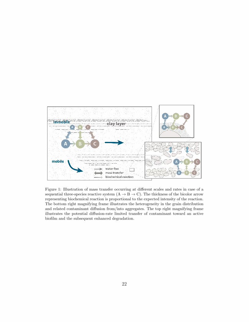
Figure 1: Illustration of mass transfer occurring at different scales and rates in case of asequential three-species reactive system (A → B → C). The thickness of the bicolor arrowrepresenting biochemical reaction is proportional to the expected intensity of the reaction.The bottom right magnifying frame illustrates the heterogeneity in the grain distributionand related contaminant diffusion from/into aggregates. The top right magnifying frameillustrates the potential diffusion-rate limited transfer of contaminant toward an activebiofilm and the subsequent enhanced degradation.
22

10-5 10-3 10-1 101 10310-3
10-2
10-1
100
Tran
sitio
n P
roba
bilit
y [-]
DaII = ∞
DaII = 101
DaII = 100
DaII = 10-1
DaII = 10-2
10-5 10-3 10-1 101 10310-3
10-2
10-1
100
10-5 10-3 10-1 101 103
τ [-]
10-5
10-4
10-3
10-2
10-1
100
Tran
sitio
n P
roba
bilit
y [-]
10-5 10-3 10-1 101 103
τ [-]
10-5
10-4
10-3
10-2
10-1
100
Final State:Species 1, immobile zone
Final State:Species 1, mobile zone
Final State:Species 2, mobile zone
Final State:Species 2, immobile zone
a. b.
c. d.
Figure 2: Impact of the second Damkohler number on the transition probability of aparticle initially being species 1 in the mobile domain: (a) probability to stay in the initialstate after a time t; (b) probability to be transferred to species 1 in the immobile domain;(c) probability to turn into species 2 in the mobile domain; and (d) probability to turninto species 2 in the immobile domain.
23

10-4 10-2 100 102 10410-3
10-2
10-1
100
Tran
sitio
n P
roba
bilit
y [-]
= 0.0 = 10-1
= 100
= 101
= 102
10-4 10-2 100 102 10410-3
10-2
10-1
100
10-4 10-2 100 102 104
τ [-]
10-4
10-3
10-2
10-1
100
Tran
sitio
n P
roba
bilit
y [-]
10-4 10-2 100 102 104
τ [-]
10-4
10-3
10-2
10-1
100
Final State:Species 1, immobile zone
Final State:Species 1, mobile zone
Final State:Species 2, mobile zone
Final State:Species 2, immobile zone
a. b.
c. d.
Figure 3: Impact of the ratio between decay rate in the mobile and immobile domainon the transition probability of a particle initially being species 1 in the mobile domain:(a) probability to stay in the initial state after a time t; (b) probability to be transferredto species 1 in the immobile domain; (c) probability to turn into species 2 in the mobiledomain; and (d) probability to turn into species 2 in the immobile domain.
24

Figure 4: Simulation setup displaying the lognormal distribution of the hydraulic conduc-tivity and first-order degradation rates of PCE, TCE, DCE and VC.
25

Figure 5: Snapshots of the plume of mobile particles illustrating the impact of degradationin the immobile domain at t=160 days (left hand frames) and t=512 days (right handframes). Blue spheres represent PCE particles; silver spheres represent TCE particles;golden spheres represent DCE particles; and red spheres represent VC particles. The sizeof the spheres are proportional to the log of the cancer potency factors related to thespecies. In other terms, the toxicity of the compounds are correlated to the particle sizes.
26

Figure 6: Snapshots of the plume of immobile particles illustrating the impact of degra-dation in the immobile domain at t=160 days (left hand frames) and t=512 days (righthand frames). Blue spheres represent PCE particles; silver spheres represent TCE parti-cles; golden spheres represent DCE particles; and red spheres represent VC particles. Thesize of the spheres are proportional to the log of the cancer potency factors related to thespecies. In other terms, the toxicity of the compounds are correlated to the particle sizes.
27
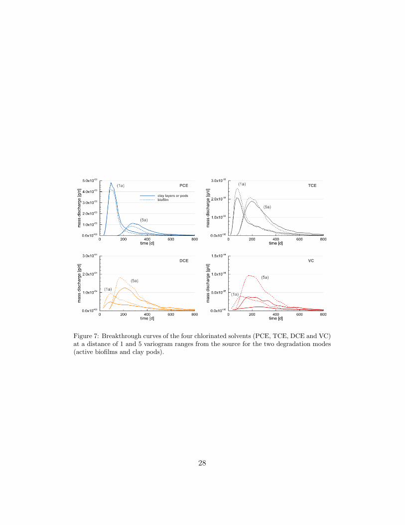
Figure 7: Breakthrough curves of the four chlorinated solvents (PCE, TCE, DCE and VC)at a distance of 1 and 5 variogram ranges from the source for the two degradation modes(active biofilms and clay pods).
28

Table 1: Physical parameters used for the illustrative simulations
Parameter ValueFlow problem
Average hydraulic gradient [−] 0.01Longitudinal dispersivity [m] 0.05Transversal dispersivity in the horizontal plane [m] 0.01Transversal dispersivity in the vertical plane [m] 0.005Porosity [−] 0.3
Heterogeneous fieldVariogram type sphericalGeometric mean of ln K [m/d] 3.55Variance of ln K 2.5Range, a [m] 10.0
Domain discretizationNumber of cells in x direction, nx × ny × nz 300 × 250 × 100Cell dimension, ∆x ×∆y ×∆z [m×m×m] 0.4 × 0.4 × 0.4
Table 2: Reaction parameters used for the illustrative simulations
Parameter ValueBiochemical (mobile domain) pce tce dce vc
Mean first-order decay, ki0 [d−1] 0.0355 0.0055 0.0352 0.0206Miminum first-order decay, min(ki0) [d−1] 0 0.001 0.00035 0.0013Maximum first-order decay, max(ki0) [d−1] 0.071 0.01 0.07 0.04First-order decay coefficient of variation [−] 0.19 0.16 0.19 0.18Yield coefficient, yi/j [mol mol−1] × 0.79 0.74 0.64Retardation factor, Ri0 [−] 7.1 2.9 2.8 1.4
Multirate Mass TransferType spherical diffusionNumber of multi-rate series, Nim 10Total capacity ration, βtot 0.17Apparent pore diffusion, Dp/a
2 0.0023
29
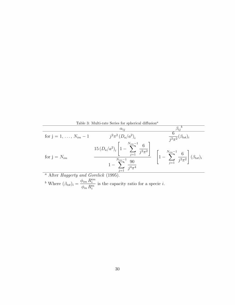
Table 3: Multi-rate Series for spherical diffusiona
αij βijb
for j = 1, . . . , Nim − 1 j2π2 (Da/a2)i
6
j2π2(βtot)i
for j = Nim
15 (Da/a2)i
[1−
Nim−1∑j=1
6
j2π2
]
1−Nim−1∑j=1
90
j4π4
[1−
Nim−1∑j=1
6
j2π2
](βtot)i
a After Haggerty and Gorelick (1995).
b Where (βtot)i =φimR
imi
φmRmi
is the capacity ratio for a specie i.
30

Appendix A. Analytical determination of the eigensystem for asimplified two-species and double porosity problem
Let us first recall the definition of our three dimensionless variables
τ =kmRm
t, (A.1)
χ =Rm kimRim km
, (A.2)
DaII =kmαRm
, (A.3)
The governing equation (12)-(11) can be written in dimensionless formfor a two-species system affected by a single rate mass transfer as:
dµm1dτ
+dµim1dτ
= −µm1 − χµim1
dµim1dτ
= Da−1II βµm1 −Da−1II µim1 − χµim1
dµm2dτ
+dµim2dτ
= µm1 − µm2 + χµim1 − χµim2
dµim2dτ
= Da−1II βµm2 −Da−1II µim2 + χµim1 − χµim2
(A.4)
This system can be written in term of matrix as in (14) defining thearchitecture matrix A and reaction matrix B as:
A =
1 1 0 00 1 0 00 0 1 10 0 0 1
(A.5)
B =
−1 −χ 0 0
Da−1II β −Da−1II − χ 0 01 χ −1 −χ0 χ Da−1II β −Da−1II − χ
, (A.6)
31

which give the matrix A−1B
A−1B =
−Da−1II β − 1 Da−1II 0 0Da−1II β −Da−1II − χ 0 0
1 0 −Da−1II β − 1 Da−1II0 χ Da−1II β −Da−1II − χ
.(A.7)
The eigensytem of a such matrix can be obtained analytically. The four
eigenvalues are given by λ =[λ1 λ1 λ2 λ2
]Twhere
λ1 =1
2
√Da−2II β
2 + 2Da−1II(Da−1II − χ+ 1
)β +
(Da−1II + χ− 1
)2+
1
2(−β − 1)Da−1II −
χ
2− 1
2,
λ2 = −1
2
√Da−2II β
2 + 2Da−1II(Da−1II − χ+ 1
)β +
(Da−1II + χ− 1
)2+
1
2(−β − 1)Da−1II −
χ
2− 1
2.
The matrix of eigenvectors is defined by:
S =
S11 0 S12 0S21 0 S22 0S31 0 S32 01 0 1 0
(A.8)
where
S1i =γiDa
−1II(
Da−1II + λi + χ) (Da−1II β + λi + 1
)Ψi
S2i =γi(
Da−1II + λi + χ)
Ψi
S3i =
((Da−1II β + λi + 2
)χ+Da−1II + λi
)Da−1II
Ψiafter the definition of Ψi and γi as:
Ψi =(−Da−1II β − λi − 1
)χ2 +
(Da−2II β
2 + ((β − 1)λi + 2 β − 1)Da−1II + λi + 1)χ
+Da−2II β,
32

γi =((Da−1II β + λi + 1
)χ+ (1 + (β + 1)λi)
(Da−1II
)+ λi
2 + λi)β (χ+ 1)Da−2II
33

Adrian NR, Robinson JA, Suflita JM. Spatial Variability in BiodegradationRates as Evidenced by Methane Production from an Aquifer Spatial Vari-ability in Biodegradation Rates as Evidenced by Methane Production froman Aquifer. Applied and environmental microbiology 1994; 60(10): 3632-3639.
Allen-King RM, Divine DP, Robin MJL, Alldredge JR, Gaylord DR. Spa-tial distributions of perchloroethylene reactive transport parameters in theBorden Aquifer, Water Resour. Res. 2006; 42(1): p. W01413.
Anderson, E., Bai, Z., Bischof, C., Blackford, S., Demmel, J., Dongarra, J.,Du Croz, J., Greenbaum, A., Hammarling, S., McKenney, A. and Sorensen,D. (1999), LAPACK Users’ Guide, Third Ed., Society for Industrial andApplied Mathematics.
Baveye, P., and A. Valocchi (1989), An evaluation of mathematical models ofthe transport of biologically reacting solutes in saturated soils and aquifers,Water Resour. Res., 25(6), 1413 1421.
Benekos, I. D., Shoemaker, C. A., and Stedinger, J. R. (2006). Probabilisticrisk and uncertainty analysis for bioremediation of four chlorinated ethenesin groundwater, Stochastic Environmental Research and Risk Assessment,21(4), 375-390. doi:10.1007/s00477-006-0071-4.
Benson, D. A. and Meerschaert, M. M. (2008). Simulation of chem-ical reaction via particle tracking: Diffusion-limited versus ther-modynamic rate-limited regimes. Water Resour. Res., 44(12), 1-7.doi:10.1029/2008WR007111.
Benson, D. a., and Meerschaert, M. M. (2009). A simple and ef-ficient random walk solution of multi-rate mobile/immobile masstransport equations, Advances in Water Resources, 32(4), 532-539.doi:10.1016/j.advwatres.2009.01.002.
Boso, F., A. Bellin, M. Dumbser (2013), Numerical simulations of solutetransport in highly heterogeneous formations: A comparison of alternativenumerical schemes, Advances in Water Resources, 52, 178-189.
Bouwer, E. J., B. E. Rittmann, and P. L. McCarty (1981), Anaerobic degra-dation of halogenated 1- and 2-carbon organic compounds, Environ. Sci.Technol., 15(5), 596599.
34

Bundt, M., Widmer, F., Pesaro, M., Zeyer, J., Blaser, P. (2001), Preferentialflow paths: biological hot spots in soils, Soil Biol. Biochem., 33, 729-738.
Burnell, D. K., J. W. Mercer, and C. R. Faust (2014), Stochastic modelinganalysis of sequential first-order degradation reactions and non-Fickiantransport in steady state plumes, Water Resour. Res., 50, doi:10.1002/2013WR013814.
Carrera, J., Sanchez-vila, X., Benet, I., Medina, A., Galarza, G., and Guimer, J. (1998). On matrix diffusion : formulations, solution methods and qual-itative effects. Hydrogeology Journal, 178–190.
Chapelle, F. (2001), Groundwater microbiology and geochemistry, Wiley, 477pp.
Clement, T. P. (1997), Technical Report PNNL-SA-11720: RT3D - A mod-ular computer code for simulating reactive multispecies transport in 3-Dimensional groundwater systems. Version 1.0. Pacific Northwest NationalLaboratory, Richland.
Clement, T. P. (2001), Generalized solution to multispecies transport equa-tions coupled with a first-order reaction network, Water Resour. Res., 37,157-163.
Cunningham, J. A., C. J. Werth, M. Reinhard, and P. V. Roberts (1997),Effects of grain-scale mass transfer on the transport of volatile organicsthrough sediments: 1. Model development, Water Resour. Res., 33(12),27132726, doi:10.1029/97WR02425.
Cunningham, J. A., and I. Mendoza-Sanchez (2006), Equivalence of two mod-els for biodegradation during contaminant transport in groundwater, Wa-ter Resour. Res., 42, W02416, doi:10.1029/2005WR004205.
Cunningham J. A. and Z. J. Fadel (2007), Contaminant degradation in phys-ically and chemically heterogeneous aquifers,J. Cont. Hydrology, 94 (3-4),293-304.
De Barros, F. P. J., Rubin, Y., and Maxwell, R. M. (2009). The con-cept of comparative information yield curves and its application torisk-based site characterization. Water Resources Research, 45(6), 1–16.doi:10.1029/2008WR007324.
35
De Barros, F. P. J., Fernandez-Garcia, D., Bolster, D., and Sanchez-Vila, X.(2013). A risk-based probabilistic framework to estimate the endpoint ofremediation: Concentration rebound by rate-limited mass transfer. WaterResour. Res., 49(4), 1929–1942. doi:10.1002/wrcr.20171.
Delay F. and J. Bodin, Time domain random walk method to simulate trans-port by advection-dispersion and matrix diffusion in fracture networks,Geophys. Res. Lett. 28 (21) (2001) 4051.
Dentz M. and B. Berkowitz, Transport behavior of a passive solute in con-tinuous time random walks and multirate mass transfer, Water Resour.Res. 39 (5) (2003) 1111–1131.
Ding, D., Benson, D. a., Paster, A. and Bolster, D. (2013).Modeling bimolecular reactions and transport in porous mediavia particle tracking. Advances in Water Resources, 53, 56–65.doi:10.1016/j.advwatres.2012.11.001.
Donado, L., X. Sanchez-Vila, M. Dentz, J. Carrera, and D. Bolster (2009),Multicomponent reactive transport in multicontinuum media, Water Re-sour. Res., 45,W11402, doi:10.1029/2008WR006823.
Edery, Y., H. Scher, and B. Berkowitz (2009), Modeling bimolecular reac-tions and transport in porous media, Geophys. Res. Lett., 36, L02407,doi:10.1029/2008GL036381.
Edery, Y., H. Scher, and B. Berkowitz (2010), Particle tracking model ofbimolecular reactive transport in porous media, Water Resour. Res., 46,W07524, doi:10.1029/2009WR009017.
Environmantal Protection Agency (EPA) (1999). Anaerobic biodegradationrates of organic chemicals on groundwater: A summary of field and labo-ratory studies. Rep. EPA S0535, Washington D.C.
Environmantal Protection Agency (EPA) (2002). Calculation and use of first-order rate constants for monitored natural attenuation studies - Groundwater issue. Rep. EPA/540/S-02/500, Washington D.C.
Falta R. W., M. B. Stacy, A. N. M. Ahsanuzzaman, M. Wang, and R. C. Earle(2007), REMChlor user’s manual, Remediation evaluation model for chlo-rinated solvents, Center for Subsurface Modeling Support Ground Water
36

and Ecosystems Restoration Division, US EPA R.S. Kerr EnvironmentalResearch Center, Ada, Oklahoma.
Feehley, C. E., C. Zheng, and F. J. Molz (2000), A dual-domain mass transferapproach for modeling solute transport in heterogeneous aquifers: Appli-cation to the Macrodisperison Experiment (MADE) site, Water ResourcesResearch, 36 (9), 2501–2515.
Fennell, D.E., A.B. Carroll, J.M. Gossett, S.H. Zinder (2001), Assessmentof indigenous reductive dechlorinating potential at a TCE-contaminatedsite using microcosms, polymerase chain reaction analysis, and site data,Environ. Sci. Technol., 35 (9), pp. 1830-1839.
Fernandez-Garcia, G. Llerar-Meza, Gmez-Hernndez, J. J. (2009), Up-scaling transport with mass transfer models: Mean behavior andpropagation of uncertainty, Water Resour. Res., 45, W10411,doi:10.1029/2009WR007764.
Fernandez-Garcia D., T. H. Illangasekare and H. Rajaram (2005), Differencesin the scale-dependence of dispersivity estimated from temporal and spatialmoments in chemically and physically heterogeneous porous media, Adv.Water Resour. Res, 28(7), 745-759.
Fernandez-Garcia D. and X. Sanchez-Vila (2011), Optimal reconstruction ofconcentrations, gradients and reaction rates from particle distributions, J.of Cont. Hydro., 120-121, 99-114.
Haggerty, R., and Gorelick, S. M. (1995). Multiple-rate mass transfer formodeling diffusion and surface reactions in media with pore-scale hetero-geneity, Water Resour. Res., 31(10), 2383-2400.
Haggerty, R., Mckenna, S. A., and Meigs, L. C. (2000). On the late-timebehavior of tracer test breakthrough curves. Water Resour. Res., 36(12),3467–3479.
Haggerty, R. (2009). STAMMT-L: Solute Transport and Multirate MassTransfer, version 3.0, user’s manual, ERMS549160.
Haggerty, R., C. F. Harvey, C. Freiherr von Schwerin, and L. C. Meigs (2004),What controls the apparent timescale of solute mass transfer in aquifers
37

and soils? A comparison of experimental results, Water Resources Re-search, 40, W01510, doi:10.1029/2002WR001716.
Harbaugh A., E. Benta, M. Hill and M. McDonald (2000),MODFLOW 2000the US Geological Survey Modular groundwater model-user guide to mod-ularization concepts and the ground-water flow process, Open File Rep.U.S. Geol. Surv., 00–92, 121pp.
Harvey, C., and Gorelick, S. M. (2000). Rate-limited mass transfer ormacrodispersion : Which dominates plume evolution at the Macrodisper-sion Experiment (MADE) site? Water Resour. Res., 36(3), 637–650.
Haston, Z. C., and P. L. McCarty (1999), Chlorinated ethene half-velocitycoefficients (Ks) for Reductive dehalogenation, Environ. Sci. Technol., 33,223226.
Henri, C. V., and D. Fernandez-Garcia (2014), Toward efficiency in hetero-geneous multispecies reactive transport modeling: A particle-tracking so-lution for first-order network reactions, Water Resour. Res., 50, 72067230,doi:10.1002/2013WR014956.
Henri, C. V., Fernandez-Garcia, D., de Barros, F. P. J., submitted. Prob-abilistic human health risk assessment of chemical mixtures in heteroge-neous aquifers: Risk statistics, hot spots and preferential flow channels.Water Resour. Res.
Huang, H., and B. X. Hu (2000), Nonlocal nonreactive transport in heteroge-neous porous media with interregional mass diffusion, Water Resour. Res.,36(7), 1665–1675.
Kitanidis, P. K. (1994), Particle-tracking equations for the solution of theadvection-dispersion equation with variable coefficients, Water Resour.Res., 30(11), 3225–3227.
Lichtner, P. C.,S. Kelkar, and B. Robinson (2002), New form ofdispersion tensor for axisymmetric porous media with implemen-tation in particle tracking, Water Resources Research, 38, 1146,doi:10.1029/2000WR000100.
Li, Z., and M. L. Brusseau (2000), Nonideal transport of reactive solutes inheterogeneous porous media: 6. Microscopic and macroscopic approaches
38

for incorporating heterogeneous rate-limited mass transfer, Water Resour.Res., 36(10), 2853–2867.
Liu G., C. Zheng and S. Gorelick, Limits of applicability of the advection-dispersion model in aquifers containing connected high-conductivity chan-nels., Water Resources Research 40 (2004) W08308.
Llopis-Albert, C. , and Capilla, J. E. (2009). Gradual conditioning of non-Gaussian transmissivity fields to flow and mass transport data. 3. Applica-tion to the macrodispersion experiment (MADE-2) site, on Columbus AirForce Base in Mississippi (USA). J. Hydrol., 371 (14 ), 7584.
Mallawatantri, A.P., McConkey, B.G., Mulla, D.J. (1996), Characterizationof pesticide sorption and degradation in macropore linings and soil horizonsof Thatuna silt loam. J. Environ. Qual., 25, 227-235.
Maxwell, R. M., Carle, S. F., and Tompson, A. F. B. (2008). Contamina-tion, risk, and heterogeneity: on the effectiveness of aquifer remediation.Environmental Geology, 54(8), 1771–1786. doi:10.1007/s00254-007-0955-8
Michalak, A. M., and P. K. Kitanidis (2000), Macroscopic behaviour andrandom-walk particle tracking of kinetically sorbing solutes, Water Re-sour. Res., 36(8), 2133–2146.
Miralles-Wilhelm, F. and L.W. Gelhar (1996), Stochastic analysis of trans-port and decay of a solute in heterogeneous aquifers, Water Resour. Res.,32 (12), pp. 3451?3459
Mishra, B. K., and C. Mishra (1991), Kinetics of nitrification and nitratereduction during leaching of ammonium nitrate through a limed Ultisolprofile, J. Indian Soc. Soil Sci., 39, 221228.
Moler, C., and Van Loan, C. (2003). Nineteen Dubious Ways to Compute theExponential of a Matrix, Twenty-Five Years Later. SIAM Review, 45(1),3–49. doi:10.1137/S00361445024180.
Neretnieks, I. (1980), Diffusion in rock matrix: An important factor in ra-dionuclide retardation?, J. Geophys. Res., 85(B8), 4379–4397.
Painter, S., V. Cvetkovic, J. Mancillas, and O. Pensado (2008), Time domainparticle tracking methods for simulating transport with retention and first-order transformation, Water Resour. Res., 44, W01406.
39

Paster, A., D. Bolster, and D. Benson (2014), Connecting the dots: Semi-analytical and random walk numerical solutions of the diffusion-reactionequation with stochastic initial conditions, Journal of ComputationalPhysics, 263, 91-112.
Pivetz, B.E., Steenhuis, T.S. (1995), Soil matrix and macropore biodegrada-tion of 2,4-D. J. Environ. Qual., 24 (4), 564-570.
Rao, P. S. C., D. E. Rolston, R. E. Jessup, and J. M. Davidson, Solute trans-port in aggregated porous media: Theoretical and experimental evaluation,Soil Sci. Soc. Am., 1, 44, 1139–1146, 1980.
Rittmann, B. E., and P. L. McCarty (1980), Model of steady state-biofilmkinetics, Biotechnol. Bioeng., 22(11), 2343 2357.
Riva, M., A. Guadagnini, D. Fernandez-Garcia, X. Sanchez-Vila and T. Ptak(2008), Relative importance of geostatistical and transport models in de-scribing heavily tailed breakthrough curves at the Lauswiesen site, Journalof Contaminant Hydrology,101, 1–13.
Ross, S. M. (2003), Introduction to probability models, 8th ed., 755 pp.,Academic Press, Oxford.
Rubin, Y. (2003), Applied Stochastic Hydrogeology, Oxford Univ. Press,Oxford.
Rubol, S., A. Freixa, A. Carles-Brangari, D. Fernandez-Garcia c, A.M. Ro-mani b, X. Sanchez-Vila (2014), Connecting bacterial colonization to phys-ical and biochemical changes in a sand box infiltration experiment, Journalof Hydrology, 517, 317–327.
Salamon, P., D. Fernandez-Garcia, J. Gomez-Hernandez, A review and nu-merical assessment of the randomwalk particle tracking method, Jour- nalof Contaminant Hydrology 87 (1-3) (2006) 277–305.
Salamon, P., Fernandez-Garcia, D., and Gomez-Hernandez, J. J. (2006).Modeling mass transfer processes using random walk particle tracking,Water Resour. Res., 42(11), 1-14. doi:10.1029/2006WR004927.
Salamon, P., D. Fernandez-Garcia, and J. J Gomez-Hernandez (2007), Mod-eling tracer transport at the made site: The importance of heterogeneity,Water Resour. Res., 43, W08404.
40

Sandrin, S. K., M.L. Brusseau, J.J. Piatt, A.A. Boudour, W.J. Blanford, N.T.Nelson (2004), Spatial variability of in situ microbial activity: biotracertests, Ground Water, 42 (3), 374-383.
Scholl, M. A. (2000). Effects of heterogeneity in aquifer permeability andbiomass on biodegradation rate calculations-Results from numerical simu-lations. Ground Water, 38, 5, 702–712.
Soga, K., J. Page, and T. Illangasekare (2004), A review of NAPL sourcezone remediation efficiency and the mass flux approach, J. Hazard. Mater.,110(13), 13–27.
Stroo, A. Leeson, J. A. Marqusee, P. C. Johnson, C. H. Ward, M. C. Ka-vanaugh, T. C. Sale, Ch. J. Newell, K. D. Pennell, C. A. Lebron, and M.Unger (2012), Chlorinated Ethene Source Remediation: Lessons Learned,Environ. Sci. Technol. 2012, 46, 6438-6447, dx.doi.org/10.1021/es204714w.
Sun, Y., J. N. Petersen, T. P. Clement, and R. S. Skeen (1999), Developmentof analytical solutions for multispecies transport with serial and parallelreactions, Water Resources Research, 35(1), 185–190.
Sun, Y., and Buscheck, T. a. (2003). Analytical solutions for reactive trans-port of N-member radionuclide chains in a single fracture. Journal of Con-taminant Hydrology, 62–63, 695–712. doi:10.1016/S0169-7722(02)00181-X
Tompson, F. B. (1993). Numerical simulation of chemical migration in phys-ically and chemically heterogeneous porous media, Water Resour. Res.,29(11), 3709–3726.
Tsang Y. W. and C. F. Tsang, A particle-tracking method for advectivetransport in fractures with diffusion into finite matrix blocks, Water Re-sources Research 37 (3) (2001) 831–835.
Valocchi, A., and H. A. M. Quinodoz (1989), Application of the randomwalk method to simulate the transport of kinetically adsorbing solutes,Groundwater Contamination, 185, 35–42.
van Genuchten, M. T., and P. J. Wierenga, Mass transfer studies in sorbingporous media, I, Analytical solutions, Soil Sci. Soc. Am. J., 40, 473-480,1976.
41

van Genuchten, M. T. (1985), Convective-dispersive transport of solutes in-volved in sequential first-order decay reactions, Comput. Geosci., 11(2),129-147.
Vinther, F.P., Eiland, F., Lind, A.M., Elsgaard, L. (1999), Microbial biomassand numbers of denitrifiers related to macropore channels in agriculturaland forest soils. Soil Biol. Biochem., 31(4), 603-611.
Vishwanathan, H. S., B. A. Robinson, A. J. Valocchi, and I. R. Triay (1998),A reactive transport model of Neptunian migration from a potential repos-itory at Yucca Mountain, J. Hydrol., 209, 251280.
Vogel, T. M., C. S. Criddle, and P. L. McCarty, Transformations of halo-genated aliphatic compounds, Environ. Sci. Technol., 21(8), 722736, 1987.
Wen, X. H.,and J. J. Gomez-Hernandez (1996), The constant displacementscheme for tracking particles in heterogeneous aquifers, Ground Water,34 (1), 135–142.
Young, D. F., and W. P. Ball (1995), Effects of column conditions on thefirst-orde rate modeling of nonequilibrium solute breakthrough, Water Re-sources Research, 31 (9), 2181–2192.
Zhang, K., and A. D. Woodbury (2002), A Krylov finite element approach formultispecies contaminant transport in discretely fractured porous media,Adv. Water Resour., 25, 705–721.
Zinn, B., and C. F. Harvey (2003), When good statistical models of aquiferheterogeneity go bad: A comparison of flow, dispersion, and mass trans-fer in connected and multivariate Gaussian hydraulic conductivity fields,Water Resources Research, 39 (3), 1051, doi:10.1029/2001WR001146.
42