a quantitative method of tailoring spectra … a quantitative method of tailoring input spectra for...
TRANSCRIPT
EDSG REPORT NO. FR-87-72-556R15 HUGHES REF. NO. F5664
A QUANTITATIVE METHOD OF TAILORING
INPUT SPECTRA FOR RANDOM VIBRATION
SCREENS
A. J. CurtisR. D. McKain
ELECTEJUL 15 1 70
Hughes Aircraft Company DElectro-Optical and Data Systems GroupEl Segundo, CA 90245
JUNE 1987
Final Report for Period March 1983 to March 1987
APPROVED FOR PUBLIC RELEASE; DISTRIBUTION UNLIMITED
Prepared for
OFFICE OF ASSISTANT SECRETARY OF THE NAVYSHIPBUILDING AND LOGISTICS, RM&QAWASHINGTON, DC 20360-5100

UNCLASSIFIEDSECURITY CLASSIFICATION OF THIS PAGE
Form Ap~proved
REPORT DOCUMENTATION PAGE 0M6No. 070.40188
Ia. REPORT SECURITY CLASSIFICATION lb RESTRICTIVE MARKINGSUNCLASSIFIED
2a. SECURITY CLASSIFICATION AUTHORITY 3. DISTRIBUTION /AVAILABILITY OF REPORT
2b. DECLASSIICATION /DOWNGRADING SCHEDULE Approved for public release; distributionunlimited.
4. PERFORMING ORGANIZATION REPORT NUMBER(S) S. MONITORING ORGANIZATION REPORT NUMBER(S)
HAC Ref. No. F5664 FR-87-12-556R N/A
6a. NAME OF PERFORMING ORGANIZATION I 6b. OFFICE SYMBOL 7a. NAME OF MONITORING ORGANIZATIONElectro-Optical and Data Sys- (If applicable) Office of Assistant Secretary of the Navytems Group, Hughes Aircraft Co. Shipbuilding and Logistics, RM&QA6c. ADDRESS (City, State, and ZIPCode) 7b. ADDRESS(City, State, and ZIPCode)
El Segundo, CA 90245 Washington, DC 20360-5100
8a. NAME OF FUNDING/SPONSORING 8b. OFFICE SYMBOL 9. PROCUREMENT INSTRUMENT IDENTIFICATION NUMBERORGANIZATION (ifapplicable) nrc ubrN01-4C29Office of Naval Research ONR 01123 Contract Number N00014-84-C-2294
8c. ADDRESS (City, State, and ZIP Code) 10. SOURCE OF FUNDING NUMBERS800 N. Quincy Street PROGRAM PROJECT TASK WORK UNITArlington, VA 22217 ELEMENT NO. NO. NO ACCESSION NO.
N68342 Z-1050 N/A N/A11. TITLE (include Security Classification)
A Quantitative Method of Tailoring Input Spectra for Random Vibration Screens
12. PERSONAL AUTHOR(S)Curtis, Allen J. and McKain, Richard D.
13a. TYPE OF REPORT 13b. TIME COVERED 14. DATE OF REPORT (Year, Month, Day) iS. PAGE COUNTFinal FROMMflr9 TI1ar 1987 June 198716. SUPPLEMENTARY NOTATION
S 17. COSATI CODES 18. SUBJECT TERMS (Conltinue onl reverser if necessary and iderrtify by block number)FIELD GROUP SUB-GROUP
;114 02
BSTRACT (Continue on reverse if necessary and identify by block number)
This report presents a rational method by which an effective random vibration screen maybe developed efficiently and quantitatively. In summary, a Flaw Precipitation Threshold(FPT) was derived from measurements of vibration res3onse at known flaw locations.Responses were measured on a variety-of modern electronic and electro-mechanical equip-ment, manufactured by five different manufacturers, during ongoing vibration screens. Avibration screen can be tailored for a piece of equipment by performing a global vibrationresponse survey and adjusting the input spectra so that the responses fall within the FPT.
i/I
20 DISTRIBUTIONNIAVAILABILITY OF ABSTRACT 21 ABSTRACT SECURITY CLASSIFICATIONIUNCLASSIFIEDIUNLIMiTED 0 SAME AS RPT 0 OTIC USERS Unclassified
22a NAME OF RESPONSIBLE INDIVIDUAL 22b TELEPHONE (Include Area Code) -..-IC- SYMBOL
.D... Patterson (202) 692-1748 S L) RM&QADD Form 1473, JUN 86 Previous editions are obsolete SECURITY CLASSIFICATION OF THIS DAGE
UNCLASSIFIED�
!7
Z,• Q,• .••. Z< <_--• , • W• •¢% _ %-.-.wr.••. ..- = • .. '; '.•.,•{a_,aZ.". ". "- -. "J ". "J "."2 '... .••'

CONTENTS
Page
1.0 IN TRO DUCTIO N ............ ............................................ I
2.0 O BJECTIV ES .............................................................. 3
3.0 STUDY STRUCTURE ...................................................... 5
4.0 D A TA BA SE .......................................... ............. ..... 7
5.0 DATA PROCESSING ...................................................... 11
6.0 DATA EVALUATION ...................................................... 13
7.0 FLAW PRECIPITATION THRESHOLD (FPT) ............................... 35
8.0 rERIVATION OF A TAILORED VIBRATION SCREEN ........................ 39
9.0 VIBRATION SURVEY ........................................... 41
10.0 RECOMMENDATIONS ............................ ....................... 43
11.0 CON CLUSIO N S ........................................................... 45
APPENDIX A: VIBRATION SURVEY GUIDELINES ............................... 47
APPENDIX B: DERIVATION OF A TAILORED VIBRATION SCREEN .............. 55
APPENDIX C: EXAMPLE TAILORING OF A VIBRATION SCREEN ............... 61
Accesion ForLII CRAMlDTIC TAB 0
"By .............. ...........D :'t 'bitio /' /
Availability CodesS• Avaj. aidlor
Dist Special
__________________ _____________________Uli

ILLUSTRATIONS
Figure Page1 Basic Approach Flow Chart ................................................. 52 M anufacturer's Activities ................................................... 63 Typical Response ASIs-S-ng!e- Axis Excitation (X) .......................... 164 Typical Response ASDs (M2) Single-Axis Excitation (Y) ........................ 175 Typical Response ASDs (M2) Two-Axis Excitation (YZ) ........................ 186 Typical Response ASDs (M2)-Two-Axis Excitation (YZ) .................... 19
7 Typical Response ASDs (M12)-Three-Axis Quasi-random Excitation ............ 208 Mean Sum-ASDs-1, 2 and 3 Axis Excitations ................................. 219 Mean Sum-ASDs-Single-Axis and All .................................. .. 22
10 Envelope of Sum-ASDs-1, 2 and 3 Axis Excitations ........................... 2311 Variability (ala) of Sum-ASDs-1, 2, and 3 Axis Excitations .................... 2412 Mean Sum-ASD Response Vis-a-Vis P-9492 Input ............................. 2513 Mean Sum-ASDs-Single-Axis Excitation, All, Sets I and II ................... .2614 Variability (al/p) of Sum-ASDs-AU, Sets I and II ............................. 2715 Distribution of Failure Levels, All Failures, 20-100 Hz ......................... 2816 Distribution of Failure Levels, All Failures, 20-300 Hz ......................... 2817 Distribution of Failure Levels, All Failures, 20-500 Hz ....................... 2918 Distribution of Failure Levels, All Failures, 20-1000 Hz ........................ 2919 Distribution of Failure Levels, All Failures, 20-1500 Hz ........................ 3020 Distribution of Failure Levels, All Failures, 20-2000 Hz ................... 3021 Cumulative Failure Probability vs RMS Acceleration .......................... 3122 RMS Acceleration vs Frequency, All Faiuares ................................. 3223 RMS Acceleration vs Frequency, Set Means ....... ............... 3324 RMS Acceleration vs Frequency, 50 and 90 Percentiles ....................... 3425 Range of Mean Response Sum-ASD ....................................... 3726 RMS Acceleration vs Frequency Range for Mean Sum-ASD .................. 3827 Flowchart of Vibration Screen Derivation ...................... ....... 39
v

TABleS
Table Page
1 Vibration Data Base ........................................................ 72 Flaw Matrix/ Sequential Axes Screens ........................................ 83 Data Base by Failure Category .............................................
. ý 9
4 Flaw Precipitation Threshold RMS Acceleration Versus Cutoff Frequency ...... 36
v
vii
[• ' ' ,,•e .-.," -•'.'•_-"• ,- .,• ,.,". "--","''• ,, ':,., :', --,•-•',• "."....3,%-'' '

FOREWORD
To date, progress in understan-'ing vibration screens has been inhibited by a failure toappreciate an inherent and fundaanental difference between establishing traditional vibra-tion design (or test) requirements and establishing vibration conditions for screens.
Vibration requirements to be rused for design purposes are based on estimates or measure-ments of the vibration environmt nt of the item to be designed or whose design adequacy isto be proven. Generally, these requirements are applicable at the interface between the itemand its supporting structure, since this is the location at which the data is available. Further-more, the data can be conveniently labeled as an "input," even though it is actually anestimated response to some unknown excitation. This permits an unambiguous analysis to beperformed and test to be controlled and is, of course, helpful in defining interface require-ments. The implication of all this is that the internal responses of the item, be they high or
L low, must be survived by one means or another.To date, vibration screens have been defined in essentially the same manner as those for
design purposes. As a practical matter, this will continue to be the case for the prescriptionand control of screens. However, for the understanding and derivation of suitable screens,this is inappropriat,. The objective of a vibration screen is to precipitate i flaw, i.e., to changean undetected defect into an observable failure. It must do this without either creating flawsor damaging sound hardware. The ability of a screen to meet this objective is not a function ofthe "input" to the item, but rather of the responses within the item. It is the vibrationenvironment in the immediate vicinity of the flaw which changes it into a failure, regardlessof the input to the item. Therefore, understanding of screens must be achieved by understand-ing the environment which precipitates the flaws. The Random Vibration Screening ProcessDevelopment Program was undertaken in an effort to understand this environment andthrough this understanding, develop a process for "tailoring" vibration screening conditionsto match the characteristics of the equipment to be screened.
The Random Vibration Screening Process Development Program was originally spon-sored out of the Office of the Chief of Navy Material. After a reorganization, sponsorship wastransferred to the Office of the Assistant Secretary of the Navy, Shipbuilding and Logistics.Technical guidance was provided by Mr. D.O. Patterson (OASN) throughout the program.This report documents the performance and results of 0he study program, while the titledescribes the end product.
ix

1.0 INTRODUCTION
The Random Vibration Screening Proces-, Development Program was sponsored by the
U.S. Navy Material Command. The study program was performed by the Tactical Engineer-ing Division of Hughes Aircraft Company's Electro-Optical and Data Systems Group in El
SSegundo, CA between March 1983 and March 1987. IBM-Owego, Litton, OECO, Rockwell=Z4 and Unisys were the manufacturing participants in the study. This report describes the
performance and results of the study program. It also makes recommendations and providesguidance for the application of these results.
¶4
_ •I,K

2.0 OBJECTIVES
"The primary objective is to establish a rational method by which an effective random
vibration screen may be developed efficiently and quantitatively. A secondary objective is to
incorporate the method into the Navy Manufacturing Screening Program document,
NAVMAT P-9492, for general usage.
3

3.0 ,TUDY STRUCTURE
The essence of the study is the establishment of the Flaw Precipitation Threshold (FPT) bymeasurement of the vibration response at known flaw locations during norm.al screening.The floti chart of this approach is shown in Figure 1.
I F FFLAW AREA OF 4.- FAILURE 4_
ENVIRONMENT FAILURE LOCATION
FAILt.F'E DATA PRECIPITATION•. THRESHOLD NI,
Figure 1. Basic approach flow chart.
For the study results to be universal in application, it was necessary that the measure-nents be made on a variety of modem electronic or electro-mechanical equipment manufac-tured by several different manufacturers. From an initial list of 18 manufacturers with on-going vibration screens, five manufacturers were selected to participate with Hughes in thestudy. The number of participants was limited to five to stay within the program budget. Thefive participants were selectcd on the basis of diversity of screens and equipment. Theactivities undertaken by the manufacturers are charted in Figure 2. Two situations aredepicted. In the top lefthand block, the manufacturer already possessed a data bank of failure
data which was sufficiently complete to permit almost immediate selection of vibrationmeasurement locations. (It should be noted that detailed failure location data is seldom ofsignificance for customary monitoring of screens.) The top righcband block illustrates thesituation where failure data were gathered during ongoing screens until sufficient data toselect measurement locations were accumulated. In general, the final list of measurementlocations was selected from a combination of the two data sources.
Once sufficient measurement locations were identified for an equipment, a representativeunit was removed from the production line and instrumented with accelerometers at each
•!• identified location. The equipment was then subjected to the normal vibration screen, i.e.,
same exciter, fixture, control accelerometer locations, input spectrum, etc., and the responseaccelerometer outputs recorded on magnetic tape.
5
NOIN~
¢. .. .. 52 -:-c Ž :.-Yr -" .
*** ~ - .-. ;'. : U .- ~- L_ . . I. .

REVIW AAILALE ATACOLLECT FAILURE DATA
OREVIE O A AILABLES DAAS GENERATED BYFOR VIBRATION FAILURES 1 LVIBRATION SCREEN
LASSEMBLE FAILURE DATAIN DESIRED FORMAT
CLASSIFY AND SELECT
REVIEW WITH HAC
EINSTRUMENT SELECTEDFAILURE LOCATIONS
VIBRATE EQUIPMENTANDiRECORD RESPONSE
SEND DATATO AC
REVIEW VIBRATION DATA
o WITH HAC
REVIEW FINAL REPORT
Figure 2. Manufacturer's activities.
The vibration data recorded by each manufacturer were forwarded to Hughes for detailed
spectral analysis. It was considered important that spectral analysis of all data be performed
using common analysis parameters such as bandwidth, degrees-of-freedom, etc., thus mandat-
ing analysis of all data by Hughes. The analyzed data were-then evaluated to determine the
FPT.
6
OLA. ,., . Q,,,4
L

4.0 DATA BASE
Participating manufacturers were selected to obtain vibration response data that is suffi-ciently diverse so the study results will be universal in nature. Diversity was sought in the"'olwing areas:•
• Manufacturers-Different techniques and processes.
* Type Equipment-Radio, computer, power supply, etc.
SDeployment-Airborne, shipboard, and ground mobile. Space hardware does not havesufficient production rate to qualify for this program.
e Type Vibration-Broadband random, quasi-random, swept sinusoidal, multiaxis, etc.
Table I summarizes the diversity in the last three areas. The equipment was manufacturedby five different firms thus giving diversity in the manufacturing area.
___ TABLE 1. VIBRATION DATA BASE
Number ofSize Measurement Number of
Equipment Deployment and Weight Screen Locatiors Sum-ASDs
Digital Computer Missile 6 X 12 X 6 Controlled Spectrum 9 16Power Supply 17 lb Random, 10 to 2 kHz,
5.8 grins, 10 min/axissequentially.
Avionics Control Airborne 8 X 10 X 20 Controlled Spectrum Ran- 8 8Unit 57 lb dom, 10 to 2 kHz, 6.0 grms,
15 min normal to cards.
Digital Computer Airborne 8 X 13 X 16 Controlled Spectrum Ran- 6 941 lb dom, 10 to 2 kHz, 4.0 grms,
5 min/axis sequentially.
Power Supply Shipboard 4.5 X 6 X 15 NAVMAT P-9492, 10 min, 21 21"24 lb I axis
Inertial Naviga- Airborne 8 X 12 X15 NAVMAT P-9492, 3 axes 13 21
tion System 35 lb sequentially, 5 min/axis.
STransceiver Airborne 4.7 X 5 X 8.4 Quasi-random, Triaxial In- 18 187 lb put, 30 min, 16 to 2 kHz,
6.4 grins composite.
Control/Display Airborne 7.1 X 5.7 X 6.5 NAVMAT P-9492, dual 5 10
Unit 10 lb axis exciter, 5 min X-Yaxes and 5 min Y-Z axes, Yaxis normal to cards.
Fiber Optics/ Ground 17 X 12 X 7.7 MIL-STD 781 C, Figure 2, 12 12Electronic Boxes Mobile 35 & 37 lb 20 to 2 kHz, 6.33 grins, 10 12 12(2 Units) minutes, normal to cards.
Totals _ 104 127
t'7
%1 r, Z1%" 6: n. 1

The last two columns in Table 1 show the spread of response measurement locations and
Sum-ASDs among the pieces of equipment. The Sum-ASD is the basic vibration function used
to derive the Flaw Precipitation Threshold and is developed in Section 5.0. It is evident from
these columns th'at measurement locations and Sum-ASDs were well spread among thevarious equipment. If the equipment was sequentially screened in multiple axes prior to a
flaw precipitating, multiple Sum-ASDs were derived for that specific location. For example, a
"three axes sequentiaUly' screen, which precipitates a flaw during the second axis, dictates
two Sum-ASDs. Table 2 shows how the number of Sum-ASDs was arrived at for the
sequential axis screens.
TABLE 2. FLAW MATRIX/SEQUENTIAL AXES SCREENS
Flaw Precipitated
No. ofScreening Meas't. Sum
Equipment Axes Locations 1st Axis 2nd Axis 3rd Axis ASDs
Digital Computer/ 3, Sequence 9 5 1 3 16Power Supply not mandated.
Digital Computer 3, Sequence 6 4 1 1 9not mandated.
Inertial Navigation 3, Sequence 13 8 2 3 21System not mandated.
Control/Display X-Y axes and Data were not available to as- 10Unit Y-Z axes certain when flaws preci-
pitated. Therefore Sum-ASDswere derived for each dual-axis excitation.
I I
Failure data received from participating manufacturers were catalogued in a format to
enable selection (or rejection) of any failure for vibration measurement. The information used
to make such a selection was:
"* Is the failure type appropriate to a screen? i.e., workmanship or part, not design.
"- If so, which of a few general failure types can be used to describe it? For ample, badcomponent, poor wiring, loose hardware, etc.
"* Is the failure location accessible for vibration measurement?
" Even. though observed in a subsequent functional test, is it a reasonable judgment thatthe flaw was precipitated by vibration?
" What was the stress-history of the equipment prior to failure detection? i.e., priorscreens, etc.
8
V.~% -X-

The selectiorL decisions were jointly made with the manufacturers, generally after several
correspondences, telecons and direct meetings.The study was designed to select the measurement locations from a data base composed of •
raw manufacturing failure data accumulated during manufacturer's past and ongoing screens.No detailed failure analysis was pl inned. These failures would then be assigned to a fewbroad categories and the vibration response data evaluated to determine if the categoriesdictated different FPTs. Also, it was felt that a body of measurements overwhelmed by a
particular failure type could be biased. For the aforementioned reasons, a concerted effort wasmade to ensure that the total population of selected failures was as diversified as possible byfailure types. The diversification was inhibited by the limited body of qualified failures fromthe manufacturers, a problem which was not anticipated in the design of the study. Only 14
of the qualified failures in the data base had been categorized as other than component. Thesewere all used in the study, as shown in Table 3. However, it is believed that many of the re-maining 90 failures which had been categorized as "component" failures would have beencategorized differently if detailed failure analysis had been performed. Without detailedfailure analysis, a component is designated the culprit when it is replaced as a result of afailure detection. In all likelihood, many of these failures are caused by damage duringassembly or improper assembly.
TABLE 3. DATA BASE BY FAILURECATEGORY
NumberFailure Category of Failures
Component 90*
Mechanical Assembly 7
Mechanical Breakage 5
Wiring/PC Board 1
Wiring /Interconnect 1
104*Failure classifications taken from raw data."Component' failures probably include manycategornes.
9
-2%

5.0 DATA PROCESSING
Previous sections have described the vibration data base available to the stuidy. The datawere delivered to Hughes by the participating manufacturers as FM-FM recordings ot -heanalog accelerometer signals together with appropriate data logs to identify failure location,accelerometer sensitivity, etc. The measurements defined the vibration in each of threeorthogonai directions at each failure location. After usual checks to verify data quality, etc.,the acceleration spectral density (ASD) of each signal was obtained, using a 10 percentcotstant percentage bandwidth analyzer arid a minimum of 35 seconds averaging time. The
ASD was obtained for the frequency raznge from 20 to 2783 Hz although tape recorderSfrequency response w as good only to approxim ately 2.5 kHz. H ow ever, data evaluation w as
confined to 2 kHz. The resultant ASD was stored in digital form so that desired arithmeticoperations could be performed on individual or groups of ASDs. Most usefully for this study,it was possible to compute the average, the envelope and the standard deviation of selectedgroups of ASDs. Further, the rms acceleration within selectable frequency ranges could beobtained by integration of the ASD within those ranges. After initial evaluation of the data, itwas decided that the vibration function to be used to derive the Flaw Precipitat-on Thresholdwould be dubbed the Sum-ASD. The Sum-ASD was simply the arithmetic sum of the ASDs
W, for each of three orthogonal axes at a specific location. No consideration of coherence, phaserelationships, etc., was attempted.
Sum-ASDs were derived for each unique excitation at each failure location, yielding atotal of 127 Sum-ASDs. Of t) iese, 99 were measured during single-axis excitation, 10 duringdual-axis excitation and 18 during quasi-random three-axis excitation. Where a failure wasidentified after a screen which consisted of sequential excitations in different directions, aSum-ASD for each excitation was created for inclusion in the pool and was treated as a single-axis ASD. The Sum-ASDs were tagged so that the groups of Sum-ASDs for single-axis, two-axis and three-axis excitations could be r_,adily formed. As explained later, two trial sets,known simply as Set I and Set H, were created by randomly selecting, for each set, 20 Sum-ASDs from the 99 single-axis Sum-ASDs.
F11
g

6.0 DATA EVALUATION
As shown in Table 1, approximately 80 percent of the measurements were responses tosingle-axis excitation. Of course, there is some unknown cross-axis excitation during anyvibration excitation but hopefully this is relatively small except in a few narrow bands at
high frequencies. However, even with essentially single-axis excitation, significant cross-axisresponses may be expected for complex asymmetric structures. When multi-axis excitation isemployed one would expect multi-axis responses. It was necessary to adopt a relativelysimple function to describe the vibration at a failure location which took account of thetriaxial nature of the responses. Based on examination of the measured spectra, this turnedout to be merely the sum of the three ASE., at that point. Typical data are shown in Figures 3through 7. Each figure contains four spectra, which are the individual spectra for the threeorthogonal directions and their sum, which is referred to as the "Sum-ASD". Figures 3 and 4are from single-axis excitation while Figures 5 and 6 are from two-axis excitation and Figure 7
is from a triaxial quasi-random excitation. Figure 3 exhibits some significant cross-axisresponses in the 100-300 Hz range. However, Figure 4 must be viewed as essentially uniaxialresponse dominated by a single resonant peak at about 300 Hz. Figure 5 for two-axisexcitation shows one axis to be generally dominant although the second axis response is veryevident. However, in Figure 6, the resonant response between 350-400 Hz is essentiallyuniaxial. Figure 7 presents three very "peaky' spectra expected from early quasi-randomexciters.
While more complex methods of accounting for the triaxial nature of the responses couldbe contemplated, it was concluded that a simple sum would suffice for the purpose at hand.
The data processing described in the previous section yielded a total of 127 Sum-ASDs,i.e., the function selected to describe the vibration level which precipitated a flaw. Initialevaluation was performed to examine if the Sum-ASDs could be treated as a single populationor if there were identifiable differences between the responses to the three types of excita-tion. Since the two and three axis data each represent a single screen, i.e., a single equipment,one cannot ascribe differences too authoritatively to the differences of excitation. Rather, onemust examine whether it is plausible that the three groups can be considered subgroups of asingle population. Figure 8 shows the mean Sum-ASD for each group while Figure 9 showsthe mean Sum-ASDs for single-axis excitation and for all excitations as a single group.
Considerable variation in responses within each group were observed as shown in FiguresS10 and 11. Figure 10 is a plot of the envelope of the Sum-ASDs for each type of excitation
which may be compared to the mean values of Figure 8, while Figure 11 is a measure of thevariability within each group, i.e., the ratio of the standard deviation to the mean value at
Mf each frequency. It is interesting that while the mean Sum-ASDs for the two-axis and three-axis groups are generally higher than and lower than the single-axis group, respectively, theenvelopes of the two-axis and three-axis groups are comparable, though both lower than thesingle-axis envelope. Of course, envelopes can only increase as data samples are added. Thesmaller variabilities for two and three axis excitations in Figure 11 must be due to the singletest items of these groups.
13MD

Based on the preceding data, it was concluded that it was acceptable to include the datafrom the twvo and three axis excitations within the single axis data to form a single group,when appropriate.
Although the main thrust of the study is directed toward responses, it is interesting tocompare the mean response, i.e., mean Sum-ASD, to the input spectrum of P-9492, since thiswas the most common input spectrum used to generate the measured responses (Reference
Table 1). This is shown in Figure 12 and indicates that, on the average, amplification is of theorder of 7 to 10 dB which is considered moderate [a Q of 10 is 20 dB]. It also indicates that re-sponses above 1000 Hz decrease as much as 10 dB/octave.
As will be discussed later, a vital part of the process will be the performance of a vibrationsurvey. To conduct a survey, i.e., to sample responses, one must select the number andlocatuan of measutrement points. To derive an adequate yet reasonable number of measure-ments, two randomly chosen sets of 20 Sum-ASDs from the 99 single axis group were formed.The mean Sum-ASDs and the variability, o-/g, of these sets were compared to the total group,as shown in Figures 13 and 14, from which it was concluded that 20 locations would sufficefor a satisfactory survey.
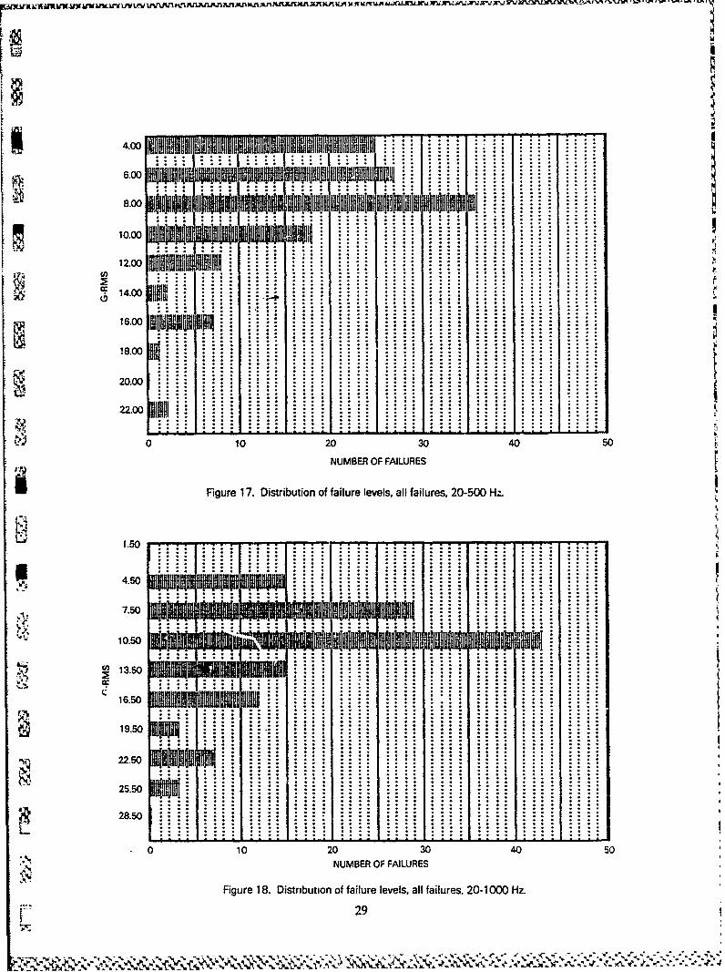
From the data presented so far, it is clear that ASDs are not entirely satisfactory to describethe Flaw Precipitation Threshold. Therefore, for each Sum-ASD, the rms accelerations from20 Hz up to the following cutoff frequencies were calculated: 100 Hz, 300 Hz, 500 Hz, 1 kHz,1.5 kHz and 2 kHz. Histograms were then prepared to examine the probability of failureversus rms level for each cut-off frequency. The histograms for all failures are shown inFigures 15 through 20. It is evident that the failures most frequently occurred at rms levelsequal to one third to one half of the maximum values, integration of the histograms ofFigures 15 through 20, and normalization to a precentage basis yield Figure 21 which can beviewed from two aspects. First, it depicts the grms level to a given cutoff frequency requiredto precipitate a given precentage of flaws. Second, since the vibration survey will maitemeasurements at potential flaw locations, it depicts the desired statistics of the survey datapoints.
From Figure 21, the following is apparent. Approximately 50 percent of the failures wereprecipitated at grms levels about one third the maximum value and 90 percent were precipi-tated at about two thirds the maximum value. An alternative view is that a fairly significantreduction in level would allow very few escapes. The potential of this figutre to define anadequate screen is discussed in the next section.
An alternate method of presentaion of these data is shown in Figure 22. Here grms isplotted versus cutoff frequency for the median (50th percentile) and 90th percentile ofcumulative failures, i.e., slices through Figure 21. The third and middle curve on Figure 22 isthe grins versus cutoff frequency for the mean Sum-ASD shown in Figure 9. Fortunately, the90th and 50th percentile curves differ from the mean by very close to 3 dB in each directionacross the frequency band. The same process used to develop Figure 22 was then applied to
14 -.
%. . .-. .. 3,... - . .

VU f l M~MR P UL W 2t lUi l.IlF1 l V-, l ,-',- .'
ii the two 20 sample randomly selected sets, to simulate the results of a vibration survey. The re-
suits for the two sets are shown in Figures 23 (meaii) and 24 (50th and 90th percentiles). Theadequacy of a 20 measurement survey is evident.
15
'7- -X._ .%'~

-- -106 _ I
r, xn cm
IIo
gs16
cm ®
.. ,.~~t a ~ . '~ **
.-, I*- *p * ~ *. - -** ~ -~. ** - - * -

Z91
11.0-k 8,
N, -w M=cEl.- iC
M 9I.E U
I-Il)
-0
IC
* ~ , ca

toc
BUII
NZI
L88
.999 c
CD~ Clciw Ew
J~. -stE >'tit -
-c6 i.
zn N -
*~6 0' 1 "
a<
:c '91 - w9~ BL~9NIB12J'-I-
18 U
- ~ V ~V

II
IwItI'
i -J6*e. 'm o o
0)C, c-i C-
I-M CD -
I -E
*S Z )C140.
U- 4)
190
0 6
.91':~8'ZIP

ooez6Z
86ZI
vc>n 0CY OT
0 C CGL6 .104; C x
E) + cD
*~te41±
-t a
caa
200

xYw> ESr 4'Wj~ C -0
_OOEZ *; 4 *
MIT' W X'
-9L6 to
.908
lag x
Lu U
_~T 0'
LL
21 =z

0ONE
W61 c
96ZI cm-0811
'SL6 OC
'Les c CID-99 U3t
-IS (fl m'
S I
10 -L~'W S5?L.-Zt N cm
ME 03-se66uj ISE 0
0: n'691 ~u_
I-,-
0'66-o.ot
LZ
9*9 c
229 U'3,
'V.
Z,9v-~ §

IWE rTT rr r ~~ T Tx :.f
M rotl -a
i'Lo
909 --
u JI ~ISE
Li .. L L LJ i.. L LQLz ~~~I~ WOq e 0
ZH/ 2 fJ~4 -1St UL~d O1~J~
J23ZU

'~A~ ~ ~ N~iU N~X~&~M-5M XAAFXrA~fl 1P~l1P7 .ALIJV i~rAJW .'L1LMMY M N ~Z ZI.
OOS 4
Ust
gzt.1 >c<
0911 ~LEL01*SL6 C'Log .0.908 CYOt .n
TEL LO U3I*w
(D.909o 3
I~~N M
-IPT
Lu 0
W.e 0j
9TE ETO C
0106
U) In 4'
NOI.LUA~O OUONVW9'49 cc
241
6*99

16OZ
86Z0811.
TT-F~-T r~ETTl'SL6'Le0 3 S iC1-908 W -J
'EEL
N 1CC CD"D oiWO 0L9z a,-Sf + >
0
E0I*61 0' V)
i' 6S1 Lz
' 601I060 CI 006-
919
0 zt'2'eCL
:1 9z-J a:
- 961 ~~"
co 10 V N x0 w 't a
21-/ 0 - IISN90 IHýL2ýdS NOIiHý112JU
25
-- ----------- -- - - - - - - - - - - - ---.. -. - , - . -..--....

ICA At 3T Tr rT 1 T~ F T% -W rI-tPI -i
1061
?SM
CLOT cc~'~
'EEL Wto U) V
'909 ->
-tic
C61 0'
8619
9,L9
8*09
Z*9t
961 CKU3
Cozc
1.191 ccL i
22
26Z ZNZl.ý .

,±wzu'iTva _v1i.z 2rj brj i w Ar wjv .xj r-wW V - v W WWI
IMT T T I T TT F T F 1 - F-
T1T S6LZT06T
zID
9I I
.909TEL tol2U w
(-~~ _jU
'Tog
'Cl,] tt~ 0U
LS~z z*VEZ LLI
'E61 C'w
0.66>0*069,19-
9S19
6'998,09 ui
TIC~
vcr
27

0.251 Ii0.75
1.25 . ......
2.75 I
3.25
475
0 10 20 30 40 50
NUMBER OF FAILURES
Figure 15. Distribution of failure levels, all failures, 20-100 Hz.
200 .. . . .. ...
8. OWO .••
,o~oo •II~tIII r.IITIIIII= ,,;,,,; i ii~rnLnriL
12.00 PIl.. . j . ...14.00
16.00
18.00
2 0 Iii' I- .
0 10 20 30 40 50NUMBER OF FAILURES
Figure 16. Distribution of failure levels, all failures. 20-300 Hz.
28
N""
14.00
$110 WN101iil 1 1 S18.00
120.00
22.00
0 10 20 30 40 50
NUMBER OF FAILURES
I Figure 17. Distribution of failure levels, all failures, 20-500 Hz.
4.50
7.50
10.50
S13.50
.................. "' .uIuE. . . . . . . . .
1090.05405
0 10 20 30 40 50.
NUMBER OF FAILURES
Figure 18. Distribution of failure levels all failures, 201000 Hz
29

12.50
6l1.50 Nl
18.50 ::
30.50
38.50
61.50
12.50
1.0 1 03 05
21.50
24.50...............................................
.........50......................................
27.50
30.50 ... *-
0 10 20 30 40 50NUMBER OF FAILURES
Figure 20. Distribution of failure levels. all failures, 20-2000 Hz.

100
.60 - 0 20-100
M 0 20-3000 20-500
0o 20-1000n-40 -• V 20-1500
0 @) 20-2000
5k2D
20
10 20 30
RMS ACCELERATION, g
Figure 21. Cumulative failure probability vs RMS acceleration.
31
4'-'

100
90%
10.0
I IU
1010 2000
CUTOFF FREQUENCY, Hz
Figure 22. RMS acceleration vs frequency, all failures.
32

S100
0
0 MEAN SUM,,SD-- SET,0 MEAN SUM ASD - SIGET AI FALUE
100 1000 2000CUTOFF FREQUENCY, Hz
L Figure 23. RMS acceleration vs frequency, set means.
R33
r-z '- r r r••' ,' r [. ,•••v••v¥ f.••~•. ~ 3k•W -1 r. '. 1 • -''.r #••-1••••• '4 jW .. mq-•rw• •• •.••.••••=. r.-r• •,

100
90%1
z0
< 10U/)
0] 0 SINGLE-AXIS FAILURES
100 1000 2000
CUTOFF FREQUENCY, Hz
Figure 24. RMS acceleration vs frequency, 50 and 90 percentiles.
34

7.0 FLAW PRECIPITATION THRESHOLD (FPT)
It is simple to postulate the existence of the Flaw Precipitation Threshold, that is, the
I vibration level sufficient to precipitate a flaw into an observable failure. Clearly, it cannot bea simple number unique to every flaw. Nor could one create a screen which would generate
* the same vibration level at every point of the item to be screened. Thus, it is necessary to de-scribe the FPT in terms of some global response of the item, permitting a rather broad rangeof responses from point to point. Thus, the FPT has evolved to be the characteristics that theglobal response of the item will exhibit under a satisfactory screen. Further, the global"response can be determined from a vibration survey in which responses are measured atapproximately 20 locations, depending on the size and complexity of the test item. Based onthe evaluation of the measured responses described in the previous section, the followingFPT is recommended for inclusion in revised guidelines for stress screening.
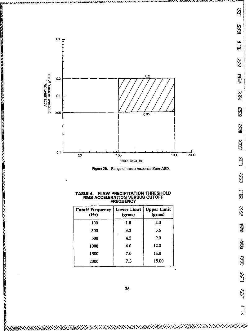
The FPT is defined in terms of the response sum acceleration spectral density (Sum-ASD)which is defined as the sum of the three response spectral densities at a point in threeorthogonal directions. Fcr a satisfactory screen, the mean Sum-ASD should be within theboundaries of the cross-hatched area of Figure 25. In addition, the rms acceleration versuscutoff frequency of the mean internal response Sum-ASD shall be as shown in Table 4 andFigure 26. Further, the 50th and 90th percentile values of the rms acceleration of individualSum-ASDs should be within +6 dB and -6 dB, respectively, of the actual measured values.
It will be noted that the upper limit in Figure 25 has been set to the straightlineapproximation of the measured value plotted in Figure 12. In addition, the upper limit inFigure 26 has been set to the measured mean value plotted in Figure 22. In both plots, thelower limit is set 6 dB lower. It is appropriate to set the upper limit to the measured valuesince the measurements were made at locations where flaws had indeed been precipitated,
* i.e., there is no need to exceed that value. It then remains to select and justify a lower limit.503 Figure 21 indicates that the reduction in flaws precipitated by a 6 dB reduction in response
might approach 20 percent if every measurement represented exactly the minimum vibrationlevel required to precipitate the failure which occurred at that point. Unfortunately, littlespecific data is available to substantiate a lower limit. However, data prepared by J. Popolo forthe third IES ESSEH Conference, September 1984, showed that 3 grins was as effective as 6grs in flushing out bad solder joints thoughineffective in flushingout unsecuredcompon-ents, for which 6 grins was only 30 percent effective at 10 minutes. A Hughes program whichhad been using 3 grins screening level was recently changed to a 6 grins level. Both levels
~ were excited by a quasi-random three-axis shaker. The effects of the change, if any, have beenvery difficult to identify from either factory or field failure data. This suggests no dramaticdifference between 3 and 6 grins. Therefore, it is believed the upper and lower limits of Table4 and Figures 25 and 26 will provide satisfactory bands within which to develop the requiredscreen.
'4 35
! .
! ~.'._
1.0
Z 00.20.2
0
P U)
i-l0 0.1
(20.05 00
F.-.n
01 ,,!,, †††††††††20 100 1000 2000
FREQUENCY, Hz
Figure25. Range of mean response Sum-ASD.
TABLE 4. FLAW PRECIPITATION THRESHOLDRMS ACCELERATION VERSUS CUTOFF
FREQUENCY
Cutoff Frequency Lower Limit Upper Limit)(Hz) (grins) (grinS)
100 1.0 2.0
300 3.3 6.6
500 4.5 9.0
1000 6.0 12.0
1500 7.0 14.0
2000 7.5 15.00
36

* 100
WU 10
100 1000 2000CUTOFF FREQUENCY, Hz
Figure 26. RMS acceleration vs frequency range for mean Sum-ASD.
37

8.0 DERIVATION OF A TAILORED VIBRATION SCREEN
I ~ With the FPT defined as described in the last section, it is now appropriate to describe theprocess to derive a suitable vibration screen. The process steps are outlined in the flowchartof Figure 27. Details of the process are included in Appendix B.
I! NEED TOSPRESCRIBE
VIBRATION SCREEN
FACILTY ~ EETBSUEj-~- PCR HPFIXTURE SELCR AELIEN I4 SPECTRU'M LEVEL
TEST SPECIMEN-SETU EE
SELECT 20MEASUREMENT PTS PERFORM VIBRATION INSTRUMENTATION
SELECT LEVEL SURVEY (APP A) DATA ACQUISITIONREDUCTION
I CALCULATEASO ANALYSIS GLOBAL DATA MASSAGING
RESPONSES (APP B)
DEVELOPFPT TAILOREDSCREEN
COFRMATION
I Figure 27. Flowchart of vibration screen derivation.
Using Figure 27 as a reference, once the need for a vibration screen has been determined,the basic configuration for the screen must be defined. The hardware portion of the configur-ation includes the equipment to be screened, a vibration facility, and a fixture attaching theequipment to the vibration facility. The basic configuration should also include a proposedscreening input spectrum from which the tailored spectrum will be derived.
A vibration survey should then be performed using a test specimen structurally represen-tative of the equipment to be screened. The vibration facility and fixture should replicate theconfiguration of the actual screen. The object of the survey is to acquire triaxial accelerationresponses at approximately 20 measurement locations within the test specimen. Guidelinesfor performing the vibration survey are presented in Appendix A.
The acceleration response data from the survey should be reduced to Sum-ASL.s fcr eachmeasurement location. These Su~m-ASDs will bc averaged to form a mean Sum-ASD. TheSum-ASDs and mean Sum-ASD will then be integrated to obtain rms acceleration versus
39
ýN`~. J% I N N, N- N. I. I -ý1

frequency curves representing the 50th percentile (me'dian) response, 90th percentile re-sponse, and mean response. To reflect response to the proposed input spectrum, the rmsacceleration curves and the mean Sum-ASD should be scaled to compensate for the reducedexcitation level.
After scaling, the mean Sum-ASD and its rms acceleration versus frequency can becompared to the FPT curves (Figures 25 and 26). Further, it can be verified that the 50th and90th percentile rms accelerations are within approximately ±3 dB of the values from themean Sum-ASD. From this comparison, it can be determined how to tailor the input spectrumso that the test specimen responses fall within the FPT. An example of this tailoring ispresented in Appendix C.
If the responses of the test equipment are not a linear function of input leve'_, it is possiblethat the responses due to the tailored input spectrum would not fall within the FPT. For thisreason, if program schedule and budget permit, the vibration survey should be repeatedusing the tailored input spectrum. Acceleration data should be pro,.essed in the same manneras the initial vibradon survey. The results should be compared to the FPT to either validate ormodify the tailored input spectrum.
40
yk

9.0 VIBRATION SURVEY
The previous section referred to the performance of a vibration survey. If an appropriatescreen is to be developed, it is important that the vibration survey be performed in a mannerconsistent with the techniques employed to derive the Flaw Precipitation Threshold. There-fore, a set of guidelines has been prepared and is included in Appendix A of this report. It isexpected that these guidelines will also become an appendix in a future revision of NAVMAT
S~P-9492.
i
ii
MAI
41- -'

10. 0 RECOMMENDA TIONS
The objective of the study program described in this report was to develop a rational,
quantitative method of tailoring a vibration screen to fit the characteristics of the equipmentto be screened. It is believed that the objective has been achieved. It remains to disseminatethe information to the ESSEH community so that it may be used and, if necessary, modified toimprove its utility. Within the Navy and its contractors, the recognized vehicle for dissemin-
ating ESSEH information is clearly NAVMAT P-9492. Therefore, it is recommended that a
revised version of P-9492 be published. This revision should accomplish the following in the
area of vibration screening:
1. Retain the present spectrum as a reasonable baseline screen absent other applicableexperience.
2. Mandate the performance of a vibration survey in the manner suggested in AppendixA of this report.
3. Include Appendix A as an appendix in the revised version.
4. Mandate the tailoring of the screen based on the EPT of Section 8.
5. Remove the present restrictions on the vibration spectrum, particularly the impliedspectral tolerance that inhibits the use of innovative excitation methods in lieu ofelectro-dynamic vibration systems.
6. Encourage the use of innovative configurations, e.g., fixtures, unit mounting, etc.,which will generate desired internal responses and precipitate flaws.
In addition to the above "paper" action, it is also recommended that a Navy program,which is or soon will be in early production, be targeted for a trial use of the method. Further.if such a trial can be arranged, it is recommended that the originators of the method be
retained to assist and monitor the results.
43

11.0 CONCLUSIONS
The previous sections have described in some detail the development of a method oftailoring to derive a suitable random vibration screen. It is believed that the method is aviable one that will lead to a screen which is both vigorous enough to precipitate flaws andyet not so severe that "good" hardware is damaged. If anything, it is felt that the method leadsto a screening level higher than needed to precipitate the flaws.
Though it may not appear thus, every effort was made to keep the method simple andpragmatic, realizing that complexity would doom the method to obscurity. However, it isbelieved that the cost of processing the measured ASDs, which is perhaps new and complexto many potential users, should represent no more than a 15 percent increase in the cost of avibration survey which should be part of any screening program.
At the inception of the study, it was hoped to include the duration of the vibiation as a pa-rameter of the Flaw Precipitation Threshold. The reader has probably noticed that this is thefirst mention of duration. Since no parametric data on duration were available, it can only beconcluded that the typical duration of 10 minutes is still suitable.
The subject of duration does raise the question of retest criteria and, more recently,failure-free period. These topics have nothing to do with developing the appropriate screen-ing level but ar.! certainly related to the perceived success or failure of a particular screeningregimen.
Regarding retest criteria, it is generally recommended that the failure, i.e., precipitatedflaw, be repaired, the screen completed and the equipment delivered without any furthervibration screen. However, if repair involves significant teardown and rework, then arescreen, perhaps at lower level and/or shorter duration should be entertained. The contrac-tor should be permitted to treat each case on a judgement basis, (e.g., FRB or MRB action)rather than the rigid rules associated with Flight Acceptance Testing of space hardware.
Recently, it has become common for screening regimen, including vibration, to call for afailure-free period. It is believed that a call for a failure free period under vibration, whichpragmatically includes the post vibration functional test period, will be counterproductive.First, it can easily create a "do-loop" which builds up vibration time for reasons unconnected
to vibration-induced failures. Secondly, it is counter to the hard-to-remember adage thatscreening "failures" are successes and will undermine the motivatiox for effective screens.Failure-free vibration screening does little more than hasten the occurrence of the nextfailure.
45

APPENDIX AVIBRATION SURVEY GUIDELINES
i
I!

APPENDIX AA NVIBRATION SURVEY GUIDELINES
1.0 GENERAL
The vibration input to electronic hardware for an effective environmental stress screencan be derived utilizing internal response data and the Flaw Precipitation Threshold. Theseguidelines define the instrumentation, performance, data acquisition and data processingrequirements to be used to acquire the internal response data. Response data acquired in
-• conformance with the guidelines will be compatible with the data used to define the FlawPrecipitation Threshold, thus assuring the validity of the derived vibration input.
2.0 TEST CONFIGURATION
The vibration survey test configuration should replicate the configuration for the pro-posed screen.
2.1 Test Item
The test item should be. representative of hardware to be screened. It should be permissi-ble to mount accelerometers internally within the test item and accumulate vibration time onthe test hardware.
2.2 Test Level
The vibration survey should be conducted at a level between 6 and 10 dB below thebaseline screening level.
2.3 Test Strategy
The survey should be performed for each input axis or combination of input axes specifiedfor the screen. For instance, a screen performed by the sequential excitation of three ortho-gonal axes requires three surveys. A screen performed as the combination of a dual axis testand a single axis test requires two surveys. A triaxial input screen requires one survey.
The controller, control strategy, and the number ax~d location of control accelerometers
should be the same as for the proposed screening tesL.
2.4 Excitation System
- The excitation system used for the survey should be the same as for the screen.
2.5 Fixturing
The fixture, slip-plate, and head expander used for the survey should be the same as forthe screen.
47
V,

. . JI�,...,,,.,
3.0 MEASUREMENT PHILOSOPHY
3.1 Selection of Measurement Locations
In the extreme, vibration response would be measured at each component, wire connec-tion, mounting screw, etc., within the test item. This clearly is neither feasible nor desirable.What is desirable is to measure vibration responses at locations throughout the volume of thetest item that are representative of responses at a majority of the potential failure locations.
Approximately 20 locations should suffice for mapping most test items.A typical test item is shown in Figure A-1 and will be used to illustrate the selection of re- I
sponse locations. The test item is an electronic card box with cable connectors and a timemeter mounted on the front panel and transformers mounted on the rear panel. There are 1Istandard cards spread throughout the box; four heavier, stiffer cards are located in the center;and an encased, thick module is located at the rear. The cards and module have connectors onthe bottom which mate with the motherboard at the bottom of the box.
[ ~i
TRANSFORMER
ENCASED MODULE
Figure A-1. Typical test item, plan view.
Twenty measurement locations to map the Figure A-1 test item could be allocated asfollows:
0 Three locations on each of the four cards indicated by arrows. 12
* Three locations within the encased module on the component mounting surfaces. 3
- One location on front panel near connectors and time meter. 1
* Two locations on motherboard. 2 ,
* Two locations on rear panel at.diagonally opposite comers of one of the transformers. 2
20
48
-~' '.ý

The three measurement locations on the cards are depicted in Figure A-2.
i0 t TOP SUPPORTED
X TOP NOT SUPPORTED
SX
S~~II i t i i I I I I I "I i i I ,I I, I I I I I I i I
Figure A-2. Response measurement locations on rectangular card with base connector.
The locations indicated by "X" are suggested for a rectangular card with componentsmounted uniformly over the surface, supported along the short edges and a connector on thebottom. If the top of the card is supported by compression of a rubber gasket on the lid, thelocations depicted by "0" would perhaps be a better choice. A square card equally supportedon each edge could be sufficiently mapped with two locations; one in the center and theother at the middle of one edge. Obviously there are many location choices within this"typical test item and within other test items that differ significantly from the typical test itemunit. The example merely illustrates mapping of the entire volume and that engineeringjudgment must be exercised in the selection of measurement locations.
3.2 Accelerometers
3.2.1 Physical Characteristics. Accelerometers should be sr , enough so that they can bemounted in the chosen location and light enough so that they do not alter the dynamiccharacteristics of the test item. In most surveys a mix of accelerometer types can be used. Inthe example illustrated by Figure A-1, relat;vely large, heavy accelerometers could be used tomeasure the acceleration input to the connectors/time meter on the front panel. Similaraccelerometers could be used on the rear panel at diagonally opposite corners of the trans-former. Medium size and weight accelerometers could probably be used on the motherboardand stiffer cards. The standard cards normally require the smallest, lightest accelerometersavailable so as to not alter the dynamic characteristics and to find mounting space.
3.2.2 Triaxial Measurement. To develop the Flaw Precipitation Threshold, the accelerationin three orthogonal directions must be known for each chosen measurement location. Thisdoes not mandate a triaxial measurement at each location. A measurement from anotherlocation may be substituted for one of the triaxial measurements if the response is judged tobe the same over the frequency range of interest. As an example, triaxial response at the three
49
4
F.

measurement locations depicted on the card in Figure A-2 can be acquired by using fiveaccelerometers. A single accelerometer is needed at each of the three measurement locationswith the sensitive axis oriented perpendicular to the plane of the board. The in-planeresponse should be the same for all locations on the board and can be acquired by placing thetwo accelerometers wherever there is adequate space.
3.2.3 Installation. Accelerometers should measure the input to components or parts, notthe response of a particular component or pa-t. In the typical test item of Figure A-i, thismeans placing accelerometers on the boards, not the components, and on the front and rearpanels, not the parts mounted to the panels.
4.0 DATA ACQUISITION
It is assumed that the control and response acceleration data will be recorded on an analogtape recorder and playe" - back to a spectrum analyzer for data analysis. Alternatively, if thespectrum analyzer has enough data channels, the data analysis could be performed "on-line,"obviating the need to record and later play back data for spectral analysis.
4.1 Data Acquisition Equipmen.r
The data acquisition system, i.e., accelerometers, signal conditioners, and tape recorder Su
system should have a frequency response flat to ± 10 percent over the frequency range ofinterest. The system should also have sufficient dynamic range to observe and record theresponse accelerations. The system should be compatible within itself and with the dataanalysis equipment.
4.2 Tape Recorder Setup
The tape recorder speed should be sufficient to obtain the desired frequency response forthe acquired data.
For the first data acquisition run in each survey, all control accelerometers should berecorded along with the response accelerometers. For all remaining data acquisition runs ineach survey, one control accei-rometer should be recorded with the response accelerometers.The control accelerometer shibald remain the same for all remaining runs to validate repeati-bility in case of questionable response data. Also, voice or a standard time code signal, IRIG,should be recorded on a tape channel to identify the beginning and end of calibration and vi-bration runs. One channel could also be used to record the charge amplifier gain codes.
50
?74 1 'A,.
F4.3 Documentation
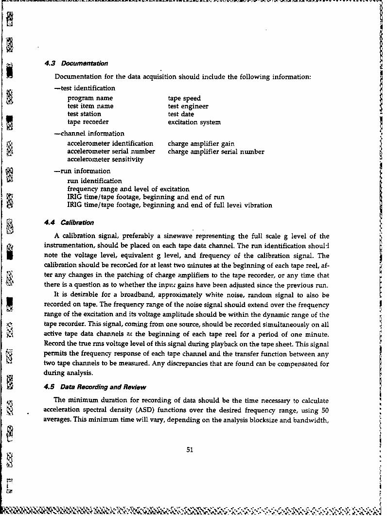
Documentation for the data acquisition should include the following information:
-test identificationprogram name tape speedtest item name test engineertest station test datetape recorder excitation system
i --channel information
accelerometer identification charge amplifier gainaccelerometer serial number charge amplifier serial numberaccelerometer sensitivity
-run informationrun identificationfrequency range and level of excitationIRIG time/tape footage, beginning and end of runIRIG time/tape footage, beginning and end of full levei vibration
4.4 Calibration
A calibration signal, preferably a sinewave representing the full scale g level of theinstrumentation, should be placed on each tape data channel. The run identification shouldnote the voltage level, equivalent g level, and frequency of the calibration signal. Thecalibration should be recorded for at least two minutes at the beginning of each tape reel, af-ter any changes in the patching of charge amplifiers to the tape recorder, or any time thatthere is a question as to whether the inpttc gains have been adjusted since the previous run.
It is desirable for a broadband, approximately white noise, random signal to also berecorded on tape. The frequency range of the noise signal should extend over the frequencyrange of the excitation and its voltage amplitude should be within the dynamic range of thetape recorder. This signal, coming from one source, should be recorded simultaneously on allactive tape data channels ac the beginning of each tape reel for a period of one minute.Record the true rms voltage level of this signal during playback on the tape sheet. This signalpermits the frequency response of each tape channel and the transfer function between anytwo tape channels to be measured. Any discrepancies that are found can be compensated forduring analysis.
4.5 Data Recording and Review
The minimum duration for recording of data should be the time necessary to calculateacceleration spectral density (ASD) functions over the desired frequency range, using 50averages. This minimum time will vary, depending on the analysis blocksize and bandwidth,
51
ýWz ww

nm2rzramunximmnXM.D.XAaA&l fwkn EAAx %XWj~AL r% Yi &-. n .rM V UrjW.! Wu jr2, ~Vý I.-- 'j ~VV k. ~IWVW WjWu W ]
the number of channels processed simultaneously, and the analyzer computational speed.The entire run should be recorded if the screen is a non-stationary process. The data shouldbe reviewed after the run to confirm that the amplitudes are appropriate, that the waveformsappear reasonable, and that the data segment is properly identified by IRIG or voice signals.The gain settings of each channel should also be verified.
5.0 DATA PROCESSING
The end result of the vibration survey should be a collection of ASD functions on a massstorage device available for Amassaging." ASD functions should be calculated for all controland response accelerometers.
5.1 Data Analysis Equipment
It is recommended that the data processing be performed by playing back the recordedanalog data to a digital Fourier spectrum analyzer. The analyzer should have the capabilitiesto calculate ASD functions, label the functions, and store the functions and labels on a massstorage device such as disc or tape. Additionally, the analyzer should be able to retrieve astored ASD, integrate the function over selected frequency ranges to obtain grins values, andprint the grins values.
5.2 Data Analysis ParametersASD functions should be calculated with 50 averages An analysis bandwidth of approxi- •
mately 5 Hz should be used for ASD calculation over the frequency range of 20 to 2000 Hz.Alternatively, a constant percentage bandwidth analyzer may be used if the bandwidth doesnot exceed 1/6th octave.
5.3 Documentation
Each ASD function should be stored with a unique identifier. A data analysis log shouldrecord the following run information and analysis parameters:
program name frequency range i-Iunit name number of averagestest date charge amp gainruidentification tape recorder channelblock size mass storage device and location numberfrequency resolution measurement I.D.
6.0 TEST PROCEDURE
The following is a procedure for performing the vibration survey. The procedure assumesthat data is recorded on analog tape and played back to a spectrum analyzer for ASDcalculation. The procedure can be modified for use with an on-line spectral analysis system.
52 ,
%'%-

The procedure also assumes that the excitation system is an electrodynamic shaker.
Therefore, for other types of excitation systems, not all steps will be relevant.
1. Record the calibration signal on all data channels of the tape recorder.
2. Record the white noise on all data .hannels of the tape recorder.
3. Attach any accelerometers and cables to the unit that require special treatment(disassembly of unit, cleanroom facilities, obstructions when installed in the fixture,etc.).
4. Create or retrieve input specification on the controller.
I5. Mount fixture to shaker table.6. Mount control accelerometer(s) to fixture and patch to the controller and data acquisi-
tion system.
7. Perform vibration dry run(s) to ensure that the control system performs properly.
8. Mou.t unit in fixture.
9. Attach remainder of response accelerometers and cables for this data run (attachLccelerometers and cables for all runs if available).
10. Patch response acce' •rometers for this run to data acquisition system.
11. Tap check all accelerometers to verify that they are properly patched to the input ofthe tape recorder and that all instrumentation functions properly.
i 12. Install all lids, covers, and unit cabling that will be on during screening.
13. Perform vibration run, recording all data.
14. Verify that the recorded data is valid before proceeding lo the next run.
15. Repeat steps 9 through 14 for remaining groups of response accelerometers.
16. Repeat steps 4 through 15 for additional surveys, if applicable.
17. Analyze recorded data to obtain ASD functions. Label and store functions on massstorage device for later retrieval and "massaging.'
UN
53
AL
Lx
p-

APPENDIX BDERIVATION OF A TAILORED VIBRATION SCREEN
S I
Ni•5

APPENDIX B
DERVIA TION OF A TAILORED VIBRATION SCREEN
A flowchart of the process to derive a tailored vibration screen is depicted in Figure B-1.Given the need to prescribe a vibration screen, certain resources are needed and, ideally,certain conditions exist. These are indicated beside the second block of Figure B-i:
1. The screening facility has been identified and is available to perform a vibrationsurvey.
2. The vibration fixture has been proven and is available for use during the survey.
3. A sample of the equipment, which is closely representative if not identical to thescreenable equipment and which can be instrumented internally, is available for theS~vibration survey.
4. Based on prior experience, a trial screening spectrum is available as the baseline fromwhich the final screen will be tailored. In lieu of prior knowledge, the spectrum of
g 4.Figure B-2 is a suitable spectrum.
5. The level by which the baseline spectrum should be reduced for the survey should beselected. (e.g., 6 to 10 dB down)
S NEED TOPRESCRIBE
:! • VIBRATION SCREEN
A FACILITY SELECT BAS IEUNE I SPECTRUM SHAPELA. SCREEURE SPECTRUM LEVEL
• ~TEST SPECIMEN
SELECT 20
MEA-3UREMENT PTS PERFORM VIBRATION - INSTRUMENTATIONSELECT LEVEL SURVEY (APP A) - DATA ACQUISITIONREDUCTION
ASD ANALYSIS-- GLOBAL 4- DATA MASSAGINGSRESPONSES (APP B)
FPT - TAILOREDSCREEN
Figure B-1 FInwrhrt nf v hnti _=nr.-,ra a4r,.1t!;n
55
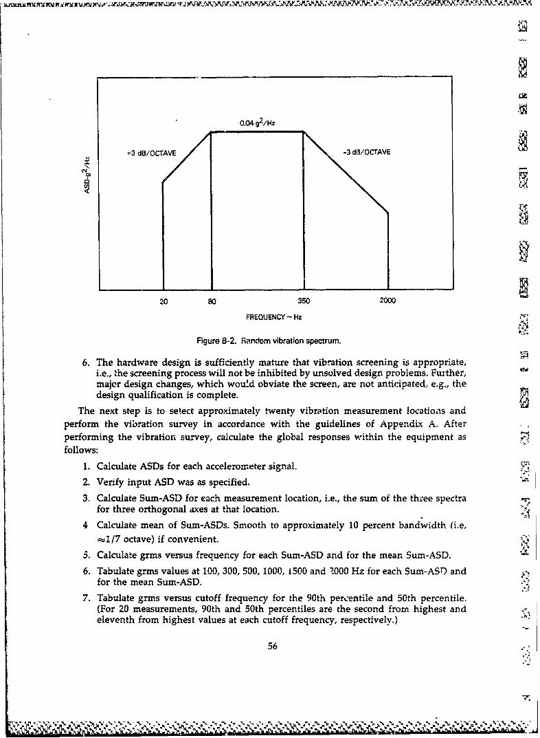
0.04 g2 /Hz
+3 dB/OCTAVE -3 dB/OCTAVE
20 80 350 2000
FREQUENCY - Hz t-j
Figure B-2. Random vibration spectrum.
6. The hardware design is sufficiently mature that vibration screening is appropriate,i.e., the screening process will not be inhibited by unsolved design problems. Fuither,major design changes, which wou~d obviate the screen, are not anticipated, e.g., thedesign qualification is complete.
The next step is to se.ect approximately twenty vibration measurement locations andperform the vibration survey in accordance with the guidelines of Appendix A. Afterperforming the vibration survey, calculate the global responses within the equipment asfollows:
1. Calculate ASDs for each accelerometer signal.
2. Verify input ASD was as specified.
3. Calculate Sum-ASD for each measurement location, i.e., the sum of the three spectrafor three orthogonal axes at that location. '
4 Calculate mean of Sum-ASDs. Smooth to approximately 10 percent bandwidth (i.e,
=1/7 octave) if convenient.
5. Calculate grms versus frequency for each Sum-ASD and for the mean Sum-ASD.
6. Tabulate grms values at 100, 300, 500, 1000, 1500 and '.000 Hz for each Sum-AST) andfor the mean Sum-ASD.
7. Tabulate grms versus cutoff frequency for the 90th percentile and 50th percentile.(For 20 measurements, 90th and 50th percentiles are the second from highest andeleventh from highest values at each cutoff frequency, respectively.)
56
-- z,

8. Scale up mean Sum-ASD by reduction factor employed during vibration survey andcompare to Figure B-3.
9. Scale up 50 percent, 90 percent and mean grms values by survey reduction factor.Compare mean grms to Figure B-4 or Table B-1. Check that 90 percent and 50 percentvalues are within 3 to 6 dB of the mean value.
10. Scale overall level, notch and/or boost input spectrum as needed to obtain reasonablematch of mean Sum-ASD and grins values to Figures B-3 and B-4 respectively. This isthe tailored screen.
11. If resources are available, repeat some or all measurements using tailored spectrum atfull level to validate the desired responses within the equipment.
1.0
S 0.2 0.2/
c• 0.1
•- n005 oo
.••20 100 1000 2000
S~FREQUENCY. Hz
•,., Figure B-3. Range of mean response Sum-ASD.
57
• ...,:" . •' ' . ' ',,,,.:,_,.,"_ ,Z'•"_2..•.'2,•.,-2 '..'.'• 2' •? • ""-,- ,-. ,_').., .2..-'.-2" ':'""-z- ''- ,.."-

100
MAXIMUM
10
_ Iw 100 1000 2000
• ~CUTOFF FREQUENCY -- IHzi6i
Figure B-4. RMS acceleration vs frequency range for mean Sum-ASD.
58-.4

TABLE B-1. FLAW PRECIPITATION THRESHOLDRMS ACCELERATION VS CUTOFF FREQUENCY
Cutoff Frequency Lower Limit Upper Limit(Hz) (grins) (grins)
100 1.0 2.0300 3.3 6.6500 4.5 9.0
1000 6.0 12.01500 7.0 14.02000 7.5 15.0
59
kn

KA
APPENDIX C
EXAMPLE TAILORING OF A VIBRATION SCREEN
i
r ..r

APPENDIX C
EXAMPLE TAILORING OF A VIBRATION SCREEN
INTRODUCTION
An example of tailoring a screen to a specific equipment, using the methods of AppendixB, is presented. The example equipment is an electro-optical package approximately 6 by 12by 12 inches in size, weighing approximately 30 pounds. The • 'ckage is composed of twomrodles, one containing optical and electronic components anu the other housing printedcircuit boards.
The 6 grins NAVMAT P-9492 specifications (Figure C-1) was proposed as the inputspectrum for screening. The excitation was provided by a two-axis electrodynamic shaker.The input was applied to both axes simultaneously and to the individual axes serially.Revised input spectra were calculated for each excitation case: X axis individually, Y axisindividually, X ana Y axes simultaneously.
TEST PERFORMANCE
Sixteen measurement locations were selected. The survey guidelines of Appendix A wereused to choose t, --,urement locations throughout the equipment that would result in a goodestimate of global structMral response. With strategic placement of accelerometers, it waspossible to acquire valid triaxial response at 16 locations using 32 accelerometers.
For each excitation, response data from all accelerometers were recorded on a 28 chann-ltape recorder. Two runs per excitation were necessary to record all of the data. The t,.duration was 2 minutes per run.
The duration is governed by the length of data necessary to calculate acceleration spectraldensity (ASD) functions with 50 averages and a 5 Hz bandwidth over a 20 to 2000 Hzfrequency range.
The NAVMAT P-9492 spectrum was selected as the trial input. The recommended excita-tion level for a screening vibration survey is 6 to 10 dB below the proposed input spectrum.For this particular test item, it was deemed satisfactory to perform the vibration survey at thefull level 6 grins NAVMAT P-9492 specification.
DATA REDUCTION AND PROCESSING
ASDs were computed from the recorded response accelerations using the previouslystated processing parameters. The ASDs for each triaxial measurement location were added toform the Sum-ASD for each location. The Sum-ASDs were then smoothed by performing acontinuous 10 percent bandwidth approximation. (Data processing can be decreased by
61

smoothing orny the mean Sum-ASD after it is obtained.) The smoothed Sum-ASDs were thenaveraged to obtain the mean Sum-ASD. The mean Sum-ASDs for the X axis, Y axis, and X-Yaxes are shown in Figures C-2, C-3, and C-4, respectively.
To summarize, the data massaging for each excitation resulted in a set of 16 smoothed
Sum-ASDs and one smoothed mean Sum-ASD. Each of these functions was then integratedover six frequency ranges: 20 to 100 Hz, 20 to 300 Hz, 20 to 500 Hz, 20 to 1000 Hz, 20 to 1500Hz, and 20 to 2000 Hz. Tables C-lA, C-1B, and C-IC list the grins values from the integrationprocess. [The data from location 4 was suspect and tot used.] For each column of the tables,the values representing the 50th percentile (median) and 90th percentile were selected. Toillustrate the selection of the 50th and 90th percentile values, refer to column 4 of TableC-lA. These are the 20 to 1000 Hz grins values from X-axis excitation. The 15 values from the
S~Sum-ASD functions were ranked by magnitude in ascending order. The 50th percentile valueis the 8th highest, 18.31 grins at location 6. The 90th percentile value is the 14th highest, 26.96
grms at location 10.
If the test had been performed at a reduced level, it would have been necessary to scalethe mean Sum-ASDs and the 50th percentile, 90th percentile, and mean sum grins values tothe proposed screening input level. However, for this particular test, the survey was per-formed at the proposed input level, obviating the scaling process.
For each excitation, the 50th percentile, 90th percentile, and mean Sum-ASD rms accelera-tion values were plotted as a function of cutoff frequency. These curves are shown in FiguresC-5 through C-7.
REVISED INPUT SPECTRA CALCULATIONComparing grms versus cutoff frequency curves for the X, Y, and X-Y excitations (Figures
C-5, C-6, and C-7, respectively) against the FPT curves of Figures C-8 and C-9, it was
observed that the overall response from all three excitations was much higher than the FPT. Itwas also observed that a disproportionate amount of response occurred in the 100 to 300 Hz
range. Therefore, to tailor each of the three screens so that the responses would be within theFPT, the overall input level should be reduced, and the input spectrum should be notched inthe 100 to 300 Hz range. This conclusion was also evident by comparison of the mean Sum-ASDs (Figures C-2 through C-4) with the recommended mean Sum-ASD range (FigureC-10).
The amount of input level reduction and spectrum notching was calculated using themean Sum-ASD. In Figure C-11, the mean Sum-ASD from X axis excitation is plotted alongwith the recommended mean Sum-ASD response range (lower cross-hatched rectangle). Toget most of the mean Sum-ASD within the recommended range, the curve was lowered 6 dB.(For ease of i'"ustration, the cross-hatched rectangle was raised 6 dB.) The region of meanSum-ASD above the +6 dB rectangle (140 to 300 Hz) was inverted to become a notch in the
62
Ilk-- NW

input spectrum. The resulting X axis input spectrum is shown in Figure C-14. Note that theoverall level has been reduced 6 dB and the spectrum is notched from 140 to 300 Hz. The in-put level from 20 to 2000 Hz was reduced to 2.92 grins from the original 6 grms. For synthesisin a digital controller, this input spectrum was approximated by the frequency and magni-
tude breakpoints listed in column 2 of Table C-2. Referring to Figure C-11, it is seen that 'he6 dB overall reduction mandates boosting of the input ASD over a small interval at each endof the FPT frequency range. However, this added complexity to the spectrum was not
considered essential to achieve an effective screen.The same calculation process was repeated for the Y axis and X-Y axes excitations. For the
Y axis, the overall level reduction was 3 dB. Spectrum notching was necessary, as seen inFigures C-12 and C-15. The revised input spectrum is 4.11 grins and is approximated by the
breakpoints in Table C-2, column 3. The X-Y input spectrum was lowered 7 dB and notched(Figure C-13), resulting in a tailored input of 2.50 grms (Figure C-16). The breakpointapproximation to Figure C-16 is given in Table C-2, column 4.
Development of these three (X, Y and X-Y) screening spectra was performed to examinethe relative merits of single and dual axis excitation. All three have been included in this
report as examples of the tailoring process.
63
X74

It
TABLE C-lA. SUM-ASD AND MEAN SUM-ASD RMSACCELERATIONS
X-Excitation
____ Frequency Range- Hertz
Identification 20-100 20-300 20-500 20-1K 20-1.5K 20-2K
Locl 1.68 4.45 6.96 8.54 9.88 10.74
Loc2 1.68 4.45 6.71 8.55 10.20 10.99
Loc3 1.67 4.45 6.67 8.27 9.64 10.45
Loc4* 4.66 5.56 5.57 5.58 5.58 5.58
Loc5 1.77 4.99 7.97 14.54 16.91 17.26
Loc6 1.63 5.78 17.24 18.31 18.54 18.66
Loc8 2.18 13.74 15.86 17.37 17.68 17.79
Loc9 2.32 14.07 17.99 20.48 21.32 21.72
LoclO 2.88 25.78 26.96 27.91 28.58 28.34
Locll 1.72 16.42 19.78 21.22 21.73 21.85
Loc12 2.26 28.96 29.67 34.49 34.96 35.55Loc13 2.86 21.87 24.00 29.03 30.42 30.61
Loc14 1.68 7.97 8.92 14.48 15.41 15.72
Loc15 1.99 9.53 11.29 16.07 16.94 17.31
Loc16 1.74 23.18 24.05 31.93 43.83 44.70
Loc17 1.98 13.70 15.20 34.53 35.24 35.48
Mean-Sum 2.06 15.55 17.74 22.56 24.61 24.96
Data from this location was suspect and eliminated from input spectrum calculations.
64
k~U.

TABLE C-i B. SUM-ASD AND MEAN SUM-ASD RMS ACCELERATIONSY-Excitation
Frequency Range- Hertz
Identification 20-100 20-300 20-500 20-1K 20-1.5K 20-2K
Loci 2.07 5.24 7.10 10.33 11.03 11.43
Loc2 2.07 5.07 6.91 10.14 10.90 11.27
Loc3 2.07 5.00 6.82 10.09 10.76 11.12
Loc4* 3.69 9.02 9.06 9.06 9.06 9.06
Loc5 2.00 4.99 7.44 16.48 22.95 23.12
Loc6 2.18 31.53 32.99 33.30 33.54 33.58
Loc8 2.23 7.12 10.01 14.76 15.13 15.21
Loc9 1.83 9.40 11.21 15.71 16.80 17.01
LoclO 1.84 17.94 18.84 20.54 21.54 21.60
Locll 1.80 6.66 9.82 15.80 17.00 17.08
Locl2 1.89 10.35 11.52 16.38 17.50 17.85
Loc13 1.92 14.16 16.20 21.34 22.24 22.46
Loc14 1.88 5.27 7.21 12.07 13.26 13.52Locl5 1 90 5.35 7.69 13.57 14.58 14.80
Locl6 1.59 9.58 11.05 16.23 30.86 31.18
Loc17 1.60 6.06 8.08 15.15 16.36 16.46
Mean-Sum 1.92 12.13 13.63 17.31 19.81 19.98
*Data from this location was suspect and eliminated from input spectrum calculations.
65
•,•"•'-'•,:•'/••.•ij.2•" -'.•.,.•:.,'..'.',•.• ':.'':..'.-.''..'''. -'_ "''.-"-..•."-" -''"-- - ."'.- - " -,,./ .- '.';'

TABLE C-1C. SUM-ASD AND MEAN SUM-ASD RMS
ACCELERATIONS
X-Y Excitation
Frequency Range -- Hertz
Identification 20-100 20-300 20-500 20-1K 20-1.5K 20-2K
Locd 2.75 6.49 9.69 13.15 14.59 15.49
Loc2 2.75 6.35 9.42 13.02 14.70 15.55
Loc3 2.75 6.30 9.32 12.81 14.25 15.10
Loc4* 5.92 9.72 9.75 9.75 9.73 9.75
Loc5 2.70 6.61 10.61 21.73 28.49 28.81
Loc6 2.69 30.66 35.95 36.66 36.98 37.06
Loc8 3.24 15.70 18.79 22.80 23.24 23.36
Loc9 3.05 16.44 20.52 24.76 26.30 26.50
LoclO 3.60 26.58 28.20 30.02 30.92 31.00
Locll 2.53 18.84 22.75 26.65 27.68 27.76
Loc12 3.09 28.17 29.28 35.77 36.55 37.19
Loc13 3.48 24.56 27.32 34.90 36.63 36.87
Loc14 2.57 8.53 10.37 18.00 19.36 19.70
Loc15 2.75 10.19 12.70 20.13 21.41 21.77
Loc16 2.53 24.65 26.22 36.33 54.96 55.91
Loc17 2.85 14.78 17.15 37.53 38.63 38.87
Mean-Sum 2.89 18.44 21.10 27.32 30.70 31.09
*Data from this location was suspect and eliminated from input spectrum calculations.
66
N N- %... V 5,_ N

TABLE C-2. REVISED SCREENING INPUTSPECTRA
Magnitude (g2/Hz)
Frequency 6 grins(Hz) NAVMAT X Y X-Y
20 0.0100 0.0025 0.0050 1 0.0020
80 0.0400 0.0100 0.0200 0.0080
140 0.0100 0.0080155 0.0200
160 0.0055
165 0.0043
S180 0.0050
190 0.0080
205 0.0055
210 0.0200
225 0.0062
240 0.0710
260 0.0040265 0.0040
270 0.0022
280 0.0040 0.0022
310 0.0100
320 0.0080
325 0.0200
350 0.0400 0.0100 0.0200 0.0080
2000 0.0070 0.0018 0.0035 0.0014
67
I

*w 0
4C6
I-
LL 4c
ca
z I--o
Lu IL L
m .I.-~
t- .IJ I
00
UU
00
Cu
Z I0
68

I~ Cu
IIx. U
0.3II-
(AI
0 u
~zI--
U) Cz ICD Z
M -4 CDw
I.-F
LU C.) mLa. I-
z * C.
K 0 ~cu~Ocu
I69

-w 3
I-U; wq
WI 1--
U)
z 0
UUU~ CO Z0.. LL W P
z * 4.
0-W W4
U LL.~
qb I-I- *W
IL)U 0 Ef3UJ C.) cc0 4c a Ci-
CD
-J
NX
CII 00
Cuj- I0 Iw Cuj
07

AL ~xpwirim~*
TAW4
_ _ _ _ _ _ _ _u
z I--
I -
LL4CCD
I--
Z) 0 w
IU I.- L.LL
a. i L wU LL CJx
W 0
-1 *W C.D01-115 *CU.3 L
0 CL
00CDJ
z I00
71

50
-90%
MEAN-SUM ASO
20 ....
0
9j10
5
2
1 I I I ,, i
100 300 500 1000 2000
CUTOFF FREQUENCY - Hz
Figure C-5. RMS acceleration vs frequency range, X axis.
72

90%
20 MEAN-SUM ASD
50%
w
S10
(n
5
2
100 300 500 1000 2000
CUTOFF FREQUENCY - Hz
Figure C-6. RMS acceleration vs. frequency range, Y axis.
IL
73
64*.-~-- ,.

50
MEAN-SUM ASD
50%
20
z0
Uj
-- 1
cc
2
100 300 500 1000 2000
CUTOFF FREQUENCY, Hz
Figure C-7. RMS acceleration vs frequency range, X-Y axes.
74
- ~- . ~ - - ~' a 7T

50
20
I Maximumz
Lu 10UA
U, Minimum
5
iN
2
1100 300 500 1000 2000
CUTOFF FREQUENCY - Hz
Figure C-8. RMS acceleration vs. frequency range, flaw precipitation threshold.
a:
75
3_~

-ii
50
90%20
MEAN-3UM ASD
50%L 10
5
2
100 300 500 1000 2000
CUTOFF FREQUENCY - Hz
Figure C-9. RMS acceleration vs. frequency range, flaw precipitation threshold.
76

cu
ZLUC30
-I 0C3,
CL,U )
00
I- 0
LU co
-- j
00
0 cu

I
~cc
0I--
oz
C3 CD ZD'
CL L wW .2)CD 0 xLZ U- 7
z C.3
I- W- 0 u
<- a.I-
U) 00
Cu
'4 78

I-4c
U)
L.u
U) C1-3 Z .
LIi x< Z
cr U)
1ý- z
U COZU.4 (1
0 U0
-j-J
cr 0
C33
-1 0 L) 0 3
zl 0
079

c'j
I
U)
Io wU) Iz 0-
0 <Icn
mU)
LU CV) < ZCL L LUU)l 0 z XU wT
w U LLZ L)
-j I
I-- *W CD I--.'-1 0 .3 0wLUJ .0 c
IN.
U) 0
08
80-
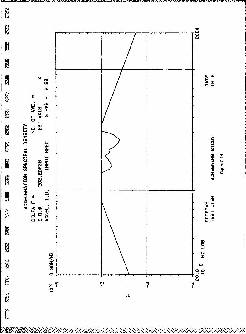
Cu
I;I
aWa.
C3u-
I-zLU M0L
U) o LL
I- I-
0 cu I C)
H 0
I-- cu Of
0.I
-j cc
0
U)
cu C')uz I III
81
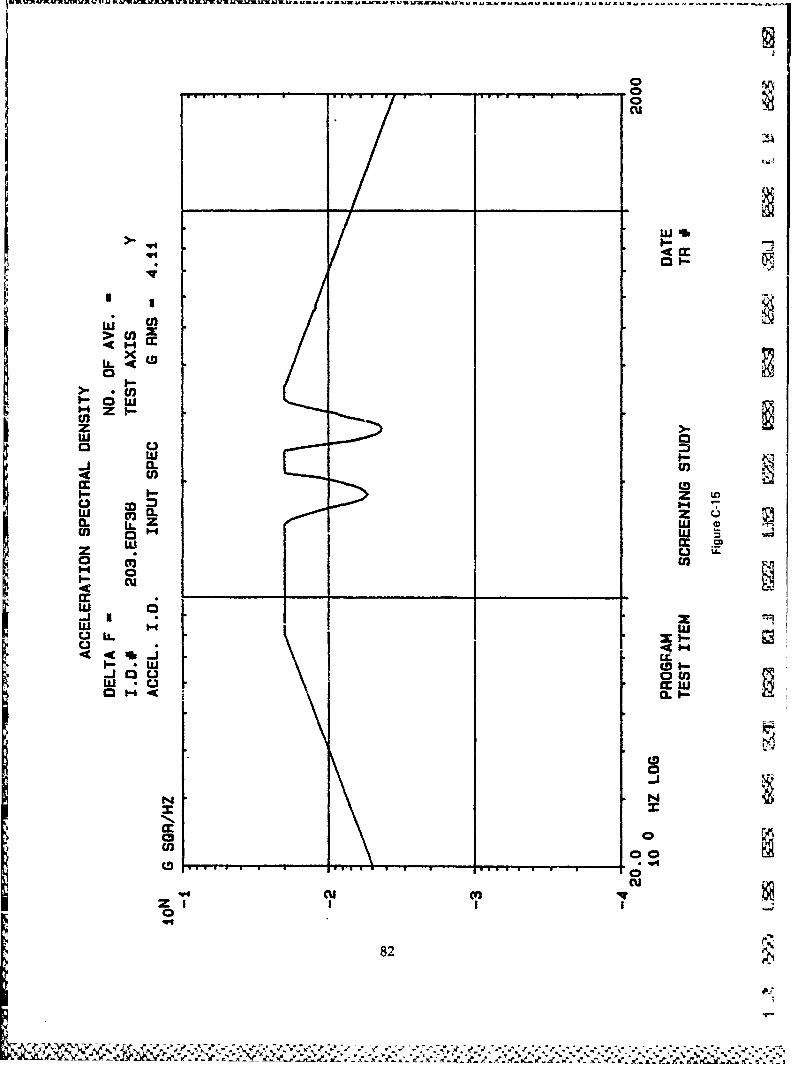
JAM rN1USMNNUJM r~maM w ' l~I X W M a a
cu
x 0-
0
z I--R.cnow
a. U
4cU) cn-biCC LD
LU 0
LL *j LU
0 m U)
)a
w 0
CDD
L- -U Lv2 C
0
82

CýC
0-
0
zLUU
m eCOC
m I Um
z- U zC.
LU cu
0 0
E3 (fL C
C3 8