Int J Comput VisDOI 10.1007/s11263-013-0644-x

A Quantitative Analysis of Current Practices in Optical FlowEstimation and the Principles Behind Them

Deqing Sun · Stefan Roth · Michael J. Black

Received: 10 January 2013 / Accepted: 10 July 2013© The Author(s) 2013. This article is published with open access at Springerlink.com

Abstract The accuracy of optical flow estimation algo-rithms has been improving steadily as evidenced by resultson the Middlebury optical flow benchmark. The typical for-mulation, however, has changed little since the work ofHorn and Schunck. We attempt to uncover what has maderecent advances possible through a thorough analysis of howthe objective function, the optimization method, and mod-ern implementation practices influence accuracy. We dis-cover that “classical” flow formulations perform surprisinglywell when combined with modern optimization and imple-mentation techniques. One key implementation detail is themedian filtering of intermediate flow fields during optimiza-tion. While this improves the robustness of classical meth-ods it actually leads to higher energy solutions, meaningthat these methods are not optimizing the original objectivefunction. To understand the principles behind this phenom-enon, we derive a new objective function that formalizes themedian filtering heuristic. This objective function includes anon-local smoothness term that robustly integrates flow esti-mates over large spatial neighborhoods. By modifying this

Portions of this work were performed when DS and MJB were atBrown University.

D. Sun (B)School of Engineering and Applied Sciences, Harvard University,Cambridge, MA, USAe-mail: dqsun@seas.harvard.edu

S. RothDepartment of Computer Science, TU Darmstadt,Darmstadt, Germanye-mail: sroth@cs.tu-darmstadt.de

M. J. BlackMax Planck Institute for Intelligent Systems,Tübingen, Germanye-mail: black@is.mpg.de

new term to include information about flow and image bound-aries we develop a method that can better preserve motiondetails. To take advantage of the trend towards video in wide-screen format, we further introduce an asymmetric pyramiddownsampling scheme that enables the estimation of longerrange horizontal motions. The methods are evaluated on theMiddlebury, MPI Sintel, and KITTI datasets using the sameparameter settings.

Keywords Optical flow estimation · Practices ·Median filtering · Non-local term · Motion boundary

1 Introduction

The field of optical flow estimation is making steady progressas evidenced by the increasing accuracy of current meth-ods on the Middlebury optical flow benchmark (Baker etal. 2007). After over 30 years of research, these methodshave obtained an impressive level of reliability and accu-racy (Wedel et al. 2008b, 2009; Werlberger et al. 2009; Xuet al. 2012; Zimmer et al. 2009). But what has led to thisprogress? The majority of today’s methods strongly resem-ble the original formulation of Horn and Schunck (HS, 1981).They combine a data term that assumes constancy of someimage property with a spatial term that models how the flowis expected to vary across the image. An objective functioncombining these two terms is then optimized. Given that thisbasic structure is unchanged since HS, what has enabled theperformance gains of modern approaches?

The paper has three parts. In the first, we perform a studyof recent optical flow methods and models. The most accu-rate methods on the Middlebury flow dataset make differentchoices about how to model the objective function, how toapproximate this model to make it computationally tractable,

123

Int J Comput Vis

(a) “Old” HS [58] (b) “New” HS (c) Classic++ (d) Classic+NL (e) Ground truth (f) First frame

Fig. 1 Estimated optical flow on the Middlebury test “Army”sequence. Left to right: a an old implementation of the Horn andSchunck (HS) method (Sun et al. 2008), b a new implementationwith current practices, c a modern implementation of a robust version,d an improved model that uses a non-local spatial term to robustly inte-

grate information over a large spatial neighborhood, e ground truth fromthe Middlebury website (downsampled and JPEG compressed; originalground truth is withheld), and f the first frame. Color coding as in (Bakeret al. 2007), shown in Fig. 4c. Average end-point error (EPE): a 0.22,b 0.12, c 0.09, and d 0.08

and how to optimize it. Since most published methods changeall of these properties at once, it can be difficult to knowwhich choices are most important. To address this, we definea baseline algorithm that is “classical”, in that it is a directdescendant of the original HS formulation, and then system-atically vary the model and method using different techniquesfrom the art. The results are surprising. We find that only asmall number of key choices produce statistically significantimprovements and that they can be combined into a very sim-ple method that achieves reasonable accuracy. More impor-tantly, our analysis reveals what makes current flow methodswork so well.

Part two examines the principles behind this success. Wefind that one algorithmic choice produces the most significantimprovements: applying a median filter to intermediate flowvalues during incremental estimation and warping (Wedelet al. 2008b, 2009). While this heuristic improves the accu-racy of the recovered flow fields, it actually increases theenergy of the objective function. This suggests that what isbeing optimized is actually a new and different objective.Using observations about median filtering and L1 energyminimization from Li and Osher (2009), we formulate a newnon-local term that is added to the original, classical objec-tive. This new term goes beyond standard local (pairwise)smoothness to robustly integrate information over large spa-tial neighborhoods. We show that minimizing this new energyapproximates the original optimization with the heuristicmedian filtering step. Note, however, that the new objectivefalls outside our definition of classical methods.

Once the median filtering heuristic is formulated as a non-local term in the objective, we immediately recognize howto modify and improve it. In part three we show how infor-mation about image structure and flow boundaries can beincorporated into a weighted version of the non-local termto prevent over-smoothing across boundaries. By incorporat-ing structure from the image, this weighted version does not

suffer from some of the errors produced by median filteringand better preserves motion boundaries. Figure 1 illustratesoptical flow estimates for a range of methods from a “basic”HS method to our proposed Classic+NL method.

Finally we observe that the classical methods all gobeyond the original HS algorithm by using a spatial pyramidto cope with large motions. The classical pyramid downsam-ples the image equally in both the horizontal and verticaldirection, typically until some minimum image dimension isreached. With today’s wide-aspect ratio video, we point outthat an asymmetric approach can be employed resulting in apyramid that downsamples more in the horizontal directionthan in the vertical one. This effectively allows the estimationof larger horizontal motions. This simple change results insignificant improvements on the wide-aspect-ratio video inthe KITTI (Geiger et al. 2012) and MPI Sintel (Butler et al.2012) datasets.

At the time of writing our previous conference paper (Sunet al. 2010a, March), the resulting approach was ranked 1stin both angular and end-point errors in the Middlebury eval-uation. At the writing of this paper (Sep. 2012), the method,Classic+NL, ranks 13th in both AAE and EPE. Several recentand high-ranking methods directly build on Classic+NL,such as layered models (Sun et al. 2010b, 2012, 2013), meth-ods with more advanced motion prior models (Chen et al.2012; Jia et al. 2011), efficient optimization schemes for thenon-local term (Krähenbühl and Koltun 2012), and better ini-tialization to deal with large displacement optical flow (Chenet al. 2013).

Compared to the conference version (Sun et al. 2010a),this paper includes many more detailed results and analy-ses. In addition to an expanded literature review we com-pare our proposed method to the closely related non-localtotal variation method (Werlberger et al. 2010). We discussthe limitations of our method in dealing with occlusions andfast moving objects. We report results on the MIT HAMA

123

Int J Comput Vis

data set (Liu et al. 2008) and find that the results are con-sistent with those on Middlebury. We also test our methodson the MPI Sintel (Butler et al. 2012) and KITTI (Geigeret al. 2012) datasets, which offer greater challenges. Usingthe same parameters tuned on the Middlebury training set,our method performs well on these new datasets, particularlyusing an asymmetric pyramid.

In summary, the contributions of this paper are to (1)analyze current flow models and methods to understandwhich design choices matter; (2) formulate and compareseveral classical objectives descended from HS using mod-ern methods; (3) formalize one of the key heuristics andderive a new objective function that includes a non-localspatial smoothness term; (4) modify this new objective toproduce a competitive method; (5) extend spatial pyramidsto exploit the extra width of high-definition and letterboxvideos. In doing so, we provide a “recipe” for others study-ing optical flow that can guide their design choices. Finally,to enable comparison and further innovation, we provide apublic Matlab implementation (http://www.cs.brown.edu/people/dqsun; last accessed 24 July 2013).

2 Previous Work

It is important to separately analyze the contributions of theobjective function that defines the problem (Sect. 2.1) and theoptimization algorithm and implementation used to minimizeit (Sect. 2.2). The HS formulation, for example, has longbeen thought to be highly inaccurate. Barron et al. (1994)reported an average angular error (AAE) of ∼30◦ on the“Yosemite” sequence. This confounds the objective functionwith the particular optimization method proposed by Hornand Schunck. Horn and Schunck noted that the correct wayto optimize their objective is by solving a system of linearequations as is common today. This was impractical on thecomputers of the day, hence they used a heuristic method.In fact, Barron et al. note that the original HS derivativeswere implemented crudely and report a modified version ofHS with AAE around 11◦. When optimized with today’smethods, the HS objective achieves surprisingly competi-tive results (Geiger et al. 2012) despite the expected over-smoothing and sensitivity to outliers. The reported accuracyof a method is jointly determined by the objective function,the optimization techniques, the implementation details, andthe parameter tuning/learning (cf. Marr 1982; Szeliski 2010).We review related research in the context of the first threeaspects below.

2.1 Models

The global formulation of optical flow introduced by Hornand Schunck (1981) relies on both brightness constancy and

spatial smoothness assumptions, but suffers from the fact thattheir quadratic formulation is not robust to outliers. Shul-man and Herve (1989) use an L1 penalty instead to preserveflow discontinuities. Black and Anandan (1996) introduce arobust framework to deal with outliers in both the data and thespatial terms. Subsequently, many different robust functionshave been explored (Brox et al. 2004; Lempitsky et al. 2008;Sun et al. 2008) and it remains unclear which is best. We referto all these spatially-discrete formulations derived from HSas “classical.” We systematically explore variations in theformulation and optimization of these approaches. The sur-prise is that the classical model, appropriately implemented,remains fairly competitive.

There are many formulations beyond the classical onesthat we do not consider here. Significant ones use orientedsmoothness (Nagel and Enkelmann 1986; Sun et al. 2008;Wedel et al. 2009; Zimmer et al. 2011, 2009), rigidity con-straints (Wedel et al. 2008a, 2009), an over-parameterizedsmoothness term (Nir et al. 2008), or image segmentation(Black and Jepson 1996; Lei and Yang 2009; Xu et al. 2008;Zitnick et al. 2005). While they deserve similar careful con-sideration, we expect many of our conclusions to carry for-ward. Note that one can select among a set of models or meth-ods for a given sequence (Mac Aodha et al. 2010), instead offinding a “best” model for all the sequences.

2.2 Methods

Many of the implementation details that are thought to beimportant date back to the early days of optical flow. Cur-rent best practices include coarse-to-fine estimation to dealwith large motions (Bergen et al. 1992; Brox et al. 2004),texture decomposition (Wedel et al. 2008a,b) or high-orderfilter constancy (Adelson et al. 1984; Brox et al. 2004; Glaeret al. 1983; Lempitsky et al. 2010; Zimmer et al. 2009) toreduce the influence of lighting changes, incremental warp-ing (Bergen et al. 1992), warping with bicubic interpolation(Lempitsky et al. 2008; Wedel et al. 2008b), temporal aver-aging of image derivatives (Horn 1986; Wedel et al. 2008b),graduated non-convexity (Blake and Zisserman 1987) to min-imize non-convex energies (Black and Anandan 1996; Sunet al. 2008), and median filtering after each incremental esti-mation step to remove outliers (Wedel et al. 2008b).

This median filtering heuristic is of particular interest asit makes non-robust methods more robust and improves theaccuracy of all methods we tested. The effect on the objectivefunction and the underlying reason for its success have notpreviously been analyzed. Least median squares estimationcan be used to robustly reject outliers in flow estimation (Bab-Hadiashar and Suter 1998), but previous work has focusedon the data term.

Related to median filtering, and our new non-local term,is the use of bilateral filtering to prevent smoothing across

123

Int J Comput Vis

motion boundaries (Xiao et al. 2006). This approach sepa-rates a variational method into two filtering update stages, andreplaces the original anisotropic diffusion process with multi-cue driven bilateral filtering. As with median filtering, thebilateral filtering step changes the original energy function.

Models that are formulated with an L1 robust penalty areoften coupled with specialized total variation (TV) optimiza-tion methods (Zach et al. 2007). Here we focus on genericoptimization methods that can apply to most models and findthat the estimated flow fields are as accurate as the reportedresults for specialized methods.

Despite recent algorithmic advances, there is a lack of pub-licly available, easy to use, and accurate flow estimation soft-ware. The GPU4Vision project (http://gpu4vision.icg.tugraz.at; last accesed 24 July 2013) has made a substantial effortto change this and provides executable files for several accu-rate methods (Wedel et al. 2008a,b, 2009; Werlberger et al.2009). The dependence on the GPU and the lack of sourcecode are limitations. Since the publication of our confer-ence paper, our public Matlab code has been used by bothresearchers to develop new optical flow algorithms (Adato etal. 2011; Chen et al. 2012, 2013; Jia et al. 2011; Krähenbühland Koltun 2012) and practitioners to use optical flow fordifferent applications (Humayun et al. 2011; Lin and Fisher2012; Niu et al. 2012). Currently other available optical-flow software includes (http://lmb.informatik.uni-freiburg.de/resources/software.php; last accessed 24 July 2013 http://people.csail.mit.edu/celiu/OpticalFlow/; last accessed 24July 2013 http://www.cse.cuhk.edu.hk/leojia/projects/flow/;last accessed 24 July 2013).

3 Classical Models

As is common to “classical” methods we only address thetwo-frame optical flow estimation problem. We write theclassical optical flow objective function in its spatially dis-crete form as

E(u, v) =∑

i, j

{ρD(I1(i, j)− I2(i +ui, j , j +vi, j ))

+ λ[ρS(ui, j −ui+1, j )+ρS(ui, j −ui, j+1)

+ ρS(vi, j −vi+1, j )+ρS(vi, j −vi, j+1)]}, (1)

where u and v are the horizontal and vertical components ofthe optical flow field to be estimated from images I1 and I2,i, j indexes a particular image pixel location, ui, j and vi, j

are elements of u and v respectively, λ is a regularizationparameter, and ρD and ρS are the data and spatial penaltyfunctions. We consider three different penalty functions: (1)the quadratic HS penalty ρ(x) = x2; (2) the Charbonnierpenalty ρ(x) = √

x2 + ε2 (Bruhn et al. 2005), a differen-tiable variant of the absolute value, the most robust con-

vex function; and (3) the Lorentzian ρ(x) = log(1 + x2

2σ 2 ),which is a non-convex robust penalty used by Black andAnandan (1996). We refer to the robust formulation with theLorentzian penalty as BA (short for Black and Anandan).Note that this classical model is related to a standard pair-wise Markov random field (MRF) based on a 4-neighborhood(Geman and Geman 1984).

In the remainder of this section we define a baselinemethod using several techniques from the literature. Thisis not the “best” method, but includes modern techniquesand will be used for comparison. We only briefly describethe main choices, which are explored in more detail in thefollowing section and the cited references.

Quantitative results are presented throughout the remain-der of the text. In all cases we report the average end-pointerror (EPE) on the Middlebury training and test sets, depend-ing on the experiment.

3.1 Baseline Methods

To gain robustness against lighting changes, we follow Wedelet al. (2008b) and apply the Rudin–Osher–Fatemi (ROF;Rudin et al. 1992) structure texture decomposition methodto pre-process the input sequences and linearly combine thetexture and structure components (in the proportion 20:1).The parameters are set according to Wedel et al. (2008b).

Optimization is performed using a standard incrementalmulti-resolution technique (e. g., Black and Anandan 1996;Brox et al. 2004) to estimate flow fields with large displace-ments. The optical flow estimated at a coarse level is usedto warp the second image toward the first at the next finerlevel, and a flow increment is calculated between the firstimage and the warped second image. The standard deviationof the Gaussian anti-aliasing filter is set to be 1√

2d, where d

denotes the downsampling factor. Each level is recursivelydownsampled from its nearest lower level. In building thepyramid, the downsampling factor is not critical as pointedout in the next section; here we use the settings of Sun et al.(2008), which uses a factor of 0.8 in the final stages of theoptimization. For the basic pyramid scheme, we adaptivelydetermine the number of pyramid levels so that the top levelhas a width or height of around 20–30 pixels. At each pyra-mid level, we perform 10 warping steps to compute the flowincrement.

At each warping step, we linearize the data term once,which involves computing terms of the type ∂

∂x I2(i+uki, j , j+

vki, j ), where ∂/∂x denotes the partial derivative in the hori-

zontal direction, uk and vk denote the current flow estimate atiteration k. As suggested by Wedel et al. (2008b), we computethe derivatives of the second image using the 5-point deriva-tive filter 1

12 [−1 8 0 − 8 1], and warp the second image andits derivatives toward the first using the current flow estimate

123

Int J Comput Vis

by bicubic interpolation. We then compute the spatial deriva-tives of the first image, compute the average of these and thecorresponding warped derivatives of the second image (cf.Álvarez et al. 2007; Horn 1986), and use these in place of∂ I2∂x . For pixels moving out of the image boundaries, we setboth their corresponding temporal and spatial derivatives tozero. After each warping step, the flow update is computed,and then we apply a 5×5 median filter to the newly computedflow field to remove outliers (Wedel et al. 2008b).

For the Charbonnier (Classic-C) and Lorentzian (Classic-L) penalty function, we use a graduated non-convexityscheme (GNC; Blake and Zisserman 1987) as described bySun et al. (2008). First, we replace the robust penalty func-tions by quadratic penalty functions and obtain a quadraticformulation of the objective function, EQ(u, v). Then we lin-early combine the quadratic penalty function with the desiredrobust penalty function and gradually change the weightingof the two terms to reach the desired robust penalty func-tion. In practice, we use a three-stage GNC scheme, with theobjective functions for the first, second, and third stages beingEQ(u, v), 1

2

(EQ(u, v)+ E(u, v)

), and E(u, v) respectively.

The output of a previous stage serves as the initialization tothe next stage. The standard deviations of the correspondingquadratic penalty function are set to be 1 for the Charbonnierpenalty and, for the Lorentzian, are taken to be the same asthe σ value used in the Lorentzian function. The same reg-ularization weight λ is used for both the quadratic and therobust objective functions.

3.2 Baseline Results

The regularization parameter λ is selected among a set ofcandidate values to achieve the best average end-point error(EPE) on the Middlebury training set. For the Charbonnierpenalty function, the candidate set is [1, 3, 5, 8, 10] and 5 isoptimal. The Charbonnier penalty uses ε = 0.001 for boththe data and the spatial term in Eq. 1. The Lorentzian usesσ = 1.5 for the data term, σ = 0.03 for the spatial term,and λ = 0.06. These parameters are fixed throughout theexperiments, except where mentioned.

Table 1 summarizes the EPE results of the basic modelwith three different penalty functions on the Middlebury testset, along with the two top performers at the time of per-forming the evaluation (considering only published paperswhen the evaluation table was generated). Table 2 providesdetailed results for each sequence. The classic formulationswith two non-quadratic penalty functions (Classic-C) and(Classic-L) achieve competitive results despite their sim-plicity. The baseline optimization of HS and BA (Classic-L)results in significantly better accuracy than previouslyreported for these models (Sun et al. 2008). Note that theanalysis also holds for the training set (Table 3).

Table 1 Models: average rank and end-point error (EPE) on the Mid-dlebury test set using different penalty functions

Avg. Rank Avg. EPE

Classic-C 34.8 0.408

HS 49.0 0.501

Classic-L 42.7 0.530

Classic-C-brightness N/A 0.726

HS-brightness N/A 0.759

Classic-L-brightness N/A 0.603

HS (Sun et al. 2008) 66.2 0.872

BA (Classic-L) (Sun et al. 2008) 59.6 0.746

Adaptive (Wedel et al. 2009) 28.5 0.401

Complementary OF (Zimmer et al. 2009) 31.6 0.485

Two state-of-the-art methods in Dec. 2010 are included for comparison.The ranking information was obtained at the writing of the paper (Sep.2012). Please refer to Table 2 for the EPE results on each sequence

Because Classic-C performs quite well despite its sim-plicity, we set it as the baseline below. Note that our baselineimplementation of HS has a lower average EPE than manymore sophisticated methods. The HS implementation hereincorporates many algorithmic and implementation detailsnot present in the original HS method; the core idea ofquadratic data and spatial terms however remains the same. Inour naming convention, one can think of the HS method hereas Classic-Q, meaning that it is the same as the Classic-Cmethod except that the data and spatial penalty terms arequadratic.

4 Practices Explored

We now systematically vary the baseline approach by incor-porating different ideas that have appeared in the literature,with the goal of illuminating which of these ideas are signif-icant. This analysis is performed on the Middlebury trainingset by changing only one property at a time. Statistical sig-nificance is determined using a Wilcoxon signed rank test(Wilcoxon 1945) between each modified method and thebaseline Classic-C method; a p value less than 0.05 indi-cates a significant difference. Each section below presentsdetailed comparisons of all these methods and then summa-rizes the results in a simple “take away message” about whatwe think are the “best practices” based on the data.

4.1 Image Pre-Processing

While it is common to talk about the brightness constancyassumption as a core feature of most optical flow algorithms,in practice many other constancy assumptions have beenused. It is common, for example, to pre-filter the imagesin a variety of ways ranging from simple smoothing to edge

123

Int J Comput Vis

Table 2 Models: average end-point error (EPE) on the Middlebury optical flow benchmark (test set)

Rank Average Army Mequon Schefflera Wooden Grove Urban Yosemite Teddy

HS 49.0 0.501 0.12 0.25 0.45 0.24 0.95 0.83 0.24 0.93

Classic-C 34.8 0.408 0.10 0.23 0.45 0.20 0.88 0.47 0.16 0.77

Classic-L 42.7 0.530 0.10 0.24 0.47 0.21 0.92 1.23 0.20 0.87

HS-brightness N/A 0.759 0.21 0.89 1.13 0.42 0.93 0.70 0.18 1.61

Classic-C-brightness N/A 0.726 0.39 0.95 1.12 0.42 0.87 0.48 0.13 1.45

Classic-L-brightness N/A 0.603 0.17 0.64 0.84 0.32 0.90 0.48 0.13 1.34

HS (Sun et al. 2008) 66.2 0.872 0.22 0.61 1.01 0.78 1.26 1.43 0.16 1.51

BA (Classic-L) (Sun et al. 2008) 59.6 0.746 0.18 0.58 0.95 0.49 1.08 1.43 0.15 1.11

Adaptive (Wedel et al. 2009) 28.5 0.401 0.09 0.23 0.54 0.18 0.88 0.50 0.14 0.65

Complementary OF (Zimmer et al. 2009) 31.6 0.485 0.10 0.20 0.35 0.19 0.87 1.46 0.11 0.60

NL-TV-NCC (Werlberger et al. 2010) 23.5 0.388 0.10 0.22 0.35 0.15 0.79 0.78 0.16 0.55

Classic++ 32.7 0.406 0.09 0.23 0.43 0.20 0.87 0.47 0.17 0.79

Classic++Gradient 33.5 0.430 0.08 0.17 0.49 0.21 0.94 0.55 0.17 0.83

Classic+NL 17.2 0.319 0.08 0.22 0.29 0.15 0.64 0.52 0.16 0.49

Classic+NL-Full 17.5 0.316 0.08 0.24 0.28 0.15 0.63 0.49 0.16 0.50

The ranking information was determined at the writing of the paper (Sep. 2012)

Table 3 Pre-processing: average end-point error (EPE) on the Mid-dlebury training set for the baseline method (Classic-C) using differentimage pre-processing techniques

Avg. EPE Significance p value

Classic-C 0.298 – –

HS 0.384 1 0.0078

Classic-L 0.319 1 0.0078

Classic-C-brightness 0.288 0 0.9453

HS-brightness 0.387 1 0.0078

Classic-L-brightness 0.325 0 0.2969

Gradient 0.305 0 0.4609

Gaussian + Dx + Dy 0.290 0 0.6406

Sobel edge magnitude(Vaudrey and Klette 2009)

0.417 1 0.0156

Laplacian (Lempitsky et al. 2010) 0.430 1 0.0078

Laplacian 1:1 0.301 0 0.6641

Gaussian pre-filtering (σ = 0.5) 0.281 0 0.5469

Texture 4:1 0.286 0 0.5312

Unnormalized texture 0.298 0 0.3750

Significance is always with respect to Classic-C. Please refer toTables 4 and 5 for the detailed results on each training sequenceBold entries highlight statistical significance

detection. For each method, we optimize the regularizationparameter λ for the training sequences. The results are sum-marized in Table 3, with details of the methods applied toindividual training sequences given in Tables 4 and 5. Thebaseline uses a non-linear pre-filtering of the images (ROF) toreduce the influence of illumination changes between frames

(Wedel et al. 2008b). Table 3 shows the effect of usingno pre-processing, resulting in the standard brightness con-stancy model (*-brightness). Classic-C-brightness actuallyachieves lower EPE on the training set than does Classic-Cbut significantly higher error on the test set (Table 1). Thisdisparity suggests overfitting to the training data and leavesopen the question as to whether the standard brightness con-stancy assumption, formulated robustly, may still competewith various types of filter/structure constancy given appro-priate training data.

Simpler alternatives, such as filter response (or high-order)constancy (Brox et al. 2004; Bruhn & Weickert 2005; Sun etal. 2008) can serve the same purpose as ROF texture decom-position. A variety of pre-filters have been used in the litera-ture, including derivative filters, Laplacians (Burt et al. 1982;Lempitsky et al. 2010), and Gaussians. Edges have also beenemphasized using the Sobel edge magnitude (Vaudrey andKlette 2009).

Gradient only imposes constancy of the gradient vector ateach pixel as proposed by Brox et al. (2004); i. e., it robustlypenalizes the Euclidean distance between image gradients.We use central difference filters (Dx = [−0.5 0 0.5] andDy = DxT ). Gaussian+Dx+Dy assumes separate bright-ness, horizontal derivative, and vertical derivative constancy.A weighted combination of robust functions applied to eachterm is used as by Sun et al. (2008). Neither of these methodsdiffer significantly from the baseline texture decomposition(Classic-C). Two methods are significantly worse: the Sobeledge magnitude (Vaudrey and Klette 2009) and Laplacianpre-filtering (5×5) as used by Lempitsky et al. (2010). Sobel

123

Int J Comput Vis

Table 4 Models and pre-processing: average end-point error (EPE) on the Middlebury training set for the classical model and different penaltyfunctions

Average Venus Dimetrodon Hydrangea RubberWhale Grove2 Grove3 Urban2 Urban3 Signif. p value

Classic-C 0.298 0.281 0.152 0.165 0.093 0.158 0.627 0.348 0.562 – –

Classic-C-brightness 0.288 0.268 0.166 0.215 0.134 0.146 0.584 0.352 0.437 0 0.9453

HS 0.384 0.337 0.219 0.189 0.118 0.204 0.688 0.463 0.853 1 0.0078

HS-brightness 0.387 0.335 0.226 0.252 0.154 0.185 0.639 0.564 0.743 1 0.0078

Classic-L 0.319 0.294 0.193 0.175 0.095 0.166 0.648 0.374 0.604 1 0.0078

Classic-L-brightness 0.325 0.292 0.207 0.274 0.145 0.158 0.588 0.451 0.484 0 0.2969

By default, the input sequences were preprocessed using ROF texture decomposition; “brightness” means no preprocessing is performed. Thestatistical significance is tested using the Wilcoxon signed rank test between each method and the baseline (Classic-C)Bold entries highlight statistical significance

Table 5 Pre-processing: average end-point error (EPE) on the Middlebury training set for the baseline method (Classic-C) using differentpre-processing techniques

Average Venus Dimetrodon Hydrangea RubberWhale Grove2 Grove3 Urban2 Urban3 Signif. p value

Classic-C 0.298 0.281 0.152 0.165 0.093 0.158 0.627 0.348 0.562 – –

Gradient 0.305 0.288 0.141 0.167 0.092 0.165 0.614 0.385 0.588 0 0.4609

Gaussian 0.281 0.268 0.146 0.226 0.141 0.137 0.582 0.335 0.413 0 0.5469

Gaussian + Dx + Dy 0.290 0.280 0.126 0.174 0.105 0.154 0.588 0.470 0.420 0 0.6406

Dx + Dy 0.301 0.286 0.122 0.166 0.099 0.161 0.616 0.443 0.518 0 1.0000

Sobel edge (Vaudreyand Klette 2009)

0.417 0.334 0.149 0.184 0.130 0.194 0.757 0.451 1.135 1 0.0156

Laplacian (Lempitskyet al. 2008)

0.430 0.374 0.170 0.176 0.096 0.175 0.756 0.464 1.232 1 0.0078

Laplacian 1:1 0.301 0.296 0.179 0.193 0.109 0.157 0.606 0.349 0.520 0 0.6641

Texture 4:1 0.286 0.271 0.159 0.175 0.100 0.154 0.587 0.349 0.490 0 0.5312

Unnormalized texture 0.298 0.279 0.152 0.166 0.092 0.158 0.623 0.348 0.563 0 0.3750

The regularization weight λ parameter was tuned for each method to achieve optimal performance. The statistical significance is tested using theWilcoxon signed rank test between each method and the baseline (Classic-C)Bold entries highlight statistical significance

edge magnitude appears to not work well on some of thesequences, particularly the synthetic ones, and may not besuitable for a general flow estimation method. Laplacian pre-filtering (5 × 5) as used by Lempitsky et al. (2010) producesgood results on “RubberWhale”, but poor ones on the syn-thetic sequences. Note that the parameters for the FusionFlowmethod (Lempitsky et al. 2010) were mainly tuned usingthe “RubberWhale” sequence. The evaluation results sug-gest room for improving the FusionFlow method by a betterpre-processing technique. Gaussian pre-filtering (σ = 0.5)performed well on the synthetic sequences, but poorly on realones. Finally, the texture-structure blending ratio is 20:1 inWedel et al. (2008b) but 4:1 in Werlberger et al. (2009). Wefind that (Texture4:1) performs better (but not significantly)on the synthetic sequences with a little degradation on thereal ones. By default, the blended result from texture decom-position is normalized to [−1, 1] by Wedel et al. (2008b)and [0, 255] in our experiment. Not doing this normalization(Unnormalized texture) has little effect.

For the Laplacian pre-filtering, we find combining the fil-tered image with the original image, in the proportion 1:1,improves accuracy significantly (Laplacian1:1). Similar tothe ROF texture decomposition, such an approach boosts thehigh frequency while suppressing the low frequency compo-nents that contain the lighting change.Good Practices: Some form of image filtering is useful butsimple derivative constancy is nearly as good as the moresophisticated texture decomposition method.

4.2 Coarse-to-Fine Estimation and GraduatedNon-Convexity (GNC)

We vary the number of warping steps per pyramid leveland find that 3 warping steps gives similar results as usingthe baseline 10 (Table 6), except on “Urban3”, which isdominated by large motion and occlusions (see Table 7 forsequence-specific results). For the coarse-to-fine pyramid,Sun et al. (2008) use a downsampling factor of 0.8 during

123

Int J Comput Vis

Table 6 Model and methods: average end-point error (EPE) on theMiddlebury training set for the baseline method (Classic-C) using dif-ferent algorithm and modeling choices

Avg. EPE Significance p value

Classic-C 0.298 — —

3 warping steps 0.304 0 0.9688

Down-0.5 0.298 0 1.0000

w/o GNC 0.354 0 0.1094

Bilinear 0.302 0 0.1016

w/o TAVG 0.306 0 0.1562

Central derivative filter 0.300 0 0.7266

7-point derivative filter(Bruhn et al. 2005)

0.302 0 0.3125

Deriv-warp 0.297 0 0.9531

Bicubic-II 0.290 1 0.0391

Deriv-warp-II 0.287 1 0.0156

Warp-deriv-II 0.288 1 0.0391

C–L (λ = 0.6) 0.303 0 0.1562

L–C (λ = 2) 0.306 0 0.1562

GC-0.45 (λ = 3) 0.292 1 0.0156

GC-0.25 (λ = 0.7) 0.298 0 1.0000

MF 3 × 3 0.305 0 0.1016

MF 7 × 7 0.305 0 0.5625

2× MF 0.300 0 1.0000

5× MF 0.305 0 0.6875

w/o MF 0.352 1 0.0078

Classic++ 0.285 1 0.0078

Please refer to Table 7 for the detailed results on each sequenceBold entries highlight statistical significance

non-convex optimization. A traditional downsampling fac-tor of 0.5 (Down-0.5), however, has nearly identical perfor-mance. Note that a larger factor means that the pyramid levelsare more similar in size and, for a pyramid with top bottomlevels of the same size, results in more pyramid levels.

Previously, Brox et al. (2004) have reported that a down-sampling factor of 0.95 produces much better results than0.5. Note that for each iterative warping estimation step,Brox et al. use successive over-relaxation (SOR) to itera-tively solve their linear system of equations and stop the iter-ation before convergence. With a downsampling factor of0.95, they effectively increase the number of iterative warp-ing steps performed by the algorithm, and this likely helpsthe overall algorithm converge. For our implementation, wesolve the linear system of equations using the Matlab built-in backslash function and obtain converged results for eachiterative warping estimation step. Under such a setting, wefind that the downsampling factor has little influence on theperformance.

Removing the GNC procedure for the Charbonnier penaltyfunction (w/o GNC) results in higher EPE on most sequencesand higher energy on all sequences (Table 8). This suggeststhat the GNC method is helpful even for the convex Char-bonnier penalty function due to the nonlinearity of the dataterm.Good Practices: The downsampling factor does not matterwhen using a convex penalty; a standard factor of 0.5 is fine.Some form of GNC is useful even for a convex robust penaltylike Charbonnier because of the nonlinear data term.

4.3 Interpolation Method and Derivatives

We find that the baseline bicubic interpolation is more accu-rate than bilinear (Table 6, Bilinear), as already reportedin previous work (Wedel et al. 2008b). Removing temporalaveraging of the gradients (w/o TAVG), using a Central dif-ference filter [−1 0 1]/2, or using a 7-point derivative filter[−1 9 − 45 0 45 − 9 1]/60 (Bruhn et al. 2005) all reduceaccuracy compared to the baseline, but not significantly.

The baseline method computes the image derivative byfirst computing the derivative of the second image, warp-ing the intermediate result toward the first image, and thenaveraging the warped result with the spatial derivative ofthe first image. Another approach is to first warp the secondimage toward the first image, compute the derivatives of thewarped image, and then perform the temporal averaging withthe spatial derivatives of the first image (Bruhn et al. 2005).We find the second approach produces similar results (Deriv-warp). However, the derivatives computed in either way areinconsistent with those implicitly interpolated by the bicubicinterpolation. Bicubic interpolation interpolates not only theimage but also the derivatives (Press et al. 2002). Because theMatlab built-in function interp2 is based on cubic convo-lution (Keys 1981) and does not provide the derivatives usedin interpolation, we use the spline-based implementation byPress et al. (2002). With the new implementation (Bicubic-II), the three different ways to compute the derivatives givevery similar EPE results, all better than the Matlab built-in function. However, the one with consistent derivatives(Bicubic-II) gives the lowest energy solution, as shown inTable 9.Good Practices: Use spline-based bicubic interpolation witha 5-point filter. Compute the derivatives during the interpo-lation to obtain the lowest energy solutions. Temporal aver-aging of the derivatives is probably worthwhile for a smallcomputational expense.

4.4 Penalty Functions

We find that the convex Charbonnier penalty performs bet-ter than the more robust, non-convex Lorentzian on both thetraining and test sets. We test using the Charbonnier for the

123

Int J Comput Vis

Table 7 Model and methods: average end-point error (EPE) on the Middlebury training set for the baseline model (Classic-C) using differentalgorithm and modeling choices

Average Venus Dimetrodon Hydrangea RubberWhale Grove2 Grove3 Urban2 Urban3 Signif. p value

Classic-C 0.298 0.281 0.152 0.165 0.093 0.158 0.627 0.348 0.562 – –

3 warping steps 0.304 0.283 0.122 0.163 0.095 0.150 0.622 0.357 0.644 0 0.9688

Down-0.5 0.298 0.280 0.152 0.166 0.092 0.158 0.626 0.349 0.562 0 1.0000

Down-0.95 0.298 0.281 0.151 0.168 0.099 0.165 0.661 0.339 0.523 0 0.9375

w/o GNC 0.354 0.303 0.160 0.171 0.105 0.183 0.835 0.316 0.759 0 0.1094

Bilinear 0.302 0.284 0.144 0.167 0.099 0.160 0.637 0.363 0.563 0 0.1016

w/o TAVG 0.306 0.288 0.149 0.167 0.093 0.163 0.647 0.345 0.593 0 0.1562

Central 0.300 0.272 0.156 0.169 0.092 0.159 0.608 0.349 0.597 0 0.7266

7-point (Bruhn et al. 2005) 0.302 0.282 0.168 0.171 0.091 0.163 0.601 0.360 0.584 0 0.3125

Deriv-warp 0.297 0.283 0.153 0.165 0.092 0.159 0.636 0.333 0.552 0 0.9531

Bicubic-II 0.290 0.276 0.132 0.152 0.083 0.142 0.624 0.338 0.571 1 0.0391

Deriv-warp-II 0.287 0.264 0.155 0.152 0.085 0.145 0.616 0.333 0.546 1 0.0156

Warp-deriv-II 0.288 0.267 0.155 0.151 0.085 0.147 0.630 0.328 0.542 1 0.0391

C–L (λ = 0.6) 0.303 0.290 0.158 0.171 0.094 0.158 0.611 0.367 0.579 0 0.1562

L–C (λ = 2) 0.306 0.281 0.174 0.173 0.096 0.164 0.662 0.343 0.557 0 0.1562

GC-0.45 (λ = 3) 0.292 0.280 0.145 0.165 0.092 0.154 0.612 0.340 0.546 1 0.0156

GC-0.25 (λ = 0.7) 0.298 0.283 0.128 0.169 0.094 0.150 0.617 0.353 0.594 0 1.0000

MF 3 × 3 0.305 0.287 0.155 0.168 0.094 0.162 0.616 0.372 0.583 0 0.1016

MF 7 × 7 0.305 0.281 0.152 0.173 0.095 0.174 0.676 0.330 0.557 0 0.5625

2× MF 0.300 0.279 0.152 0.167 0.093 0.163 0.650 0.339 0.555 0 1.0000

5× MF 0.305 0.278 0.152 0.171 0.093 0.172 0.682 0.329 0.561 0 0.6875

w/o MF 0.352 0.307 0.168 0.199 0.113 0.217 0.705 0.423 0.684 1 0.0078

Classic++ 0.285 0.271 0.128 0.153 0.081 0.139 0.614 0.336 0.555 1 0.0078

The statistical significance is tested using the Wilcoxon signed rank test between each method and the baseline (Classic-C)Bold entries highlight statistical significance

Table 8 Energy (×106, Eq. 1) for the optical flow fields computed on the Middlebury training set, evaluated using convolution-based bicubicinterpolation (Keys 1981)

Sum Venus Dimetrodon Hydrangea RubberWhale Grove2 Grove3 Urban2 Urban3

Classic-C 9.388 0.589 0.748 0.866 0.502 1.816 2.317 1.126 1.424

w/o GNC 9.689 0.593 0.750 0.870 0.506 1.845 2.518 1.142 1.465

w/o MF 8.044 0.517 0.701 0.668 0.449 1.418 1.830 1.066 1.395

Note that Classic-C uses graduated non-convexity (GNC), which reduces the energy, and median filtering, which increases it

Table 9 Energy (×106, Eq. 1) for the optical flow fields computed on the Middlebury training set, evaluated using spline-based bicubic interpolation(Press et al. 2002)

Sum Venus Dimetrodon Hydrangea RubberWhale Grove2 Grove3 Urban2 Urban3

Bicubic-II 8.761 0.552 0.734 0.835 0.481 1.656 2.167 1.061 1.275

Deriv-warp 8.917 0.559 0.745 0.840 0.484 1.682 2.201 1.073 1.333

Warp-deriv 9.035 0.563 0.745 0.845 0.486 1.694 2.238 1.117 1.347

Note the derivatives consistent with the interpolation method (Bicubic-II) produce the lowest energy solution

123

Int J Comput Vis

−20 −15 −10 −5 0 5 10 15 200

5

10

15

20

25

x

ρ(x)

CharbonnierGeneralized Charbonnier (0.45)Generalized Charbonnier (0.25)Lorentzian

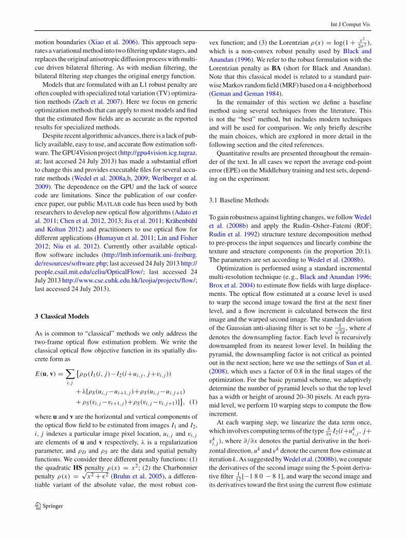
Fig. 2 Different penalty functions for the spatial terms: Charbonnier(ε = 0.001), generalized Charbonnier (a = 0.45 and a = 0.25), andLorentzian (σ = 0.03)

data term and Lorentzian for the spatial term (C–L) and viceversa (L–C). The two approaches perform better than usingthe Lorentzian for both terms but worse than using the Char-bonnier for both terms.

One reason might be that non-convex functions are moredifficult to optimize, causing the optimization scheme to finda poor local optimum. Another reason might be that theMAP estimator actually favors the “wrong” penalty func-tions (Nikolova 2007; Schmidt et al. 2010).

We investigate a generalized Charbonnier penalty func-tion ρ(x) = (x2 + ε2)a that is equal to the Charbonnierpenalty when a = 0.5, and non-convex when a < 0.5(see Fig. 2). We optimize the regularization parameter λ

again. We find a slightly non-convex penalty with a = 0.45(GC-0.45) performs consistently better than the Charbonnierpenalty, whereas more non-convex penalties (GC-0.25 witha = 0.25) show no improvement.Good Practices: The less-robust Charbonnier is preferable tothe highly non-convex Lorentzian and a slightly non-convexpenalty function (GC-0.45) is better still.

4.5 Median Filtering

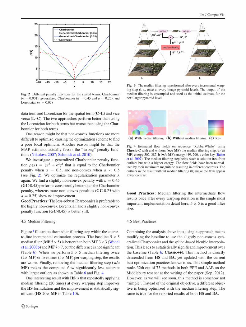
Figure 3 illustrates the median filtering step within the coarse-to-fine incremental estimation process. The baseline 5 × 5median filter (MF 5×5) is better than both MF 3×3 (Wedelet al. 2008b) and MF 7×7, but the difference is not significant(Table 6). When we perform 5 × 5 median filtering twice(2× MF) or five times (5× MF) per warping step, the resultsare worse. Finally, removing the median filtering step (w/oMF) makes the computed flow significantly less accuratewith larger outliers as shown in Table 6 and Fig. 4.

One interesting result with HS is that repeatedly applyingmedian filtering (20 times) at every warping step improvesthe HS formulation and the improvement is statistically sig-nificant (HS 20× MF in Table 10).

refine warp

median filtering

+

Fig. 3 The median filtering is performed after every incremental warp-ing step (i. e., once at every image pyramid level). The output of themedian filtering is upsampled and used as the initial estimate for thenext larger pyramid level

(a) With median filtering (b) Without median filtering (c) Key

Fig. 4 Estimated flow fields on sequence “RubberWhale” usingClassic-C with and without (w/o MF) the median filtering step. a (w/MF) energy 502, 387, b (w/o MF) energy 449, 290, c color key (Bakeret al. 2007). The median filtering step helps reach a solution free fromoutliers but with a higher energy. The flow fields have been normal-ized by their maximum magnitude resulting in different contrasts. Theoutliers in the result without median filtering (b) make the flow appearlower contrast

Good Practices: Median filtering the intermediate flowresults once after every warping iteration is the single mostimportant implementation detail here; 5 × 5 is a good filtersize.

4.6 Best Practices

Combining the analysis above into a single approach meansmodifying the baseline to use the slightly non-convex gen-eralized Charbonnier and the spline-based bicubic interpola-tion. This leads to a statistically significant improvement overthe baseline (Table 6, Classic++). This method is directlydescended from HS and BA, yet updated with the currentbest optimization practices known to us. This simple methodranks 32th out of 73 methods in both EPE and AAE on theMiddlebury test set at the writing of the paper (Sep. 2012).However, as we will see soon, this method is somehow not“simple”. Instead of the original objective, a different objec-tive is being optimized with the median filtering step. Thesame is true for the reported results of both HS and BA.

123

Int J Comput Vis

Table 10 Additional results for HS: average end-point error (EPE) on the Middlebury training set

Average Venus Dimetrodon Hydrangea RubberWhale Grove2 Grove3 Urban2 Urban3 Signif. p value

HS 0.384 0.337 0.219 0.189 0.118 0.204 0.688 0.463 0.853 – –

HS 20× MF 0.365 0.299 0.214 0.184 0.104 0.196 0.699 0.431 0.792 1 0.0469

The statistical significance is tested using the Wilcoxon signed rank test between each method and HSBold entries highlight statistical significance

5 Models Underlying Median Filtering

Our analysis reveals the practical importance of medianfiltering during optimization. This effectively denoises theintermediate flow fields, preventing gross outliers, and mak-ing even non-robust methods like HS more robust. We askwhether there is a principle underlying this heuristic?

One interesting observation is that flow fields obtainedwith median filtering have substantially higher energy thanthose without (Table 8; Fig. 4). If the median filter is helpingto optimize the objective, it should lead to lower energies.Higher energies and more accurate estimates suggest thatincorporating median filtering changes the objective functionbeing optimized.

The insight that follows from this is that the median fil-tering heuristic is related to the minimization of an objec-tive function that differs from the classical one. In particularthe optimization of Eq. 1, with interleaved median filtering,approximately minimizes

E(u, v) =∑

i, j

{ρD(I1(i, j) − I2(i + ui, j , j + vi, j ))

+λ[ρS(ui, j − ui+1, j )+ ρS(ui, j − ui, j+1)

+ρS(vi, j − vi+1, j ) + ρS(vi, j − vi, j+1)]}

+λN

∑

i, j

∑

(i ′, j ′)∈Ni, j

(|ui, j −ui ′, j ′ |+|vi, j − vi ′, j ′ |), (2)

where Ni, j is the set of neighbors of pixel (i, j) in a possiblylarge area and λN is a scalar weight. The term in braces is thesame as the flow energy from Eq. 1, while the last term is new.This non-local term (Buades et al. 2005; Gilboa and Osher2008) imposes a particular smoothness assumption within aspecified region of the flow field.1 Here we take this term tobe a 5 × 5 rectangular region to match the size of the medianfilter in Classic-C. Figure 5 shows the neighborhood for thestandard pairwise model and the non-local term.

It is usually difficult to directly optimize the objective (2)with a large spatial term. A common practice is to relax theobjective with an auxiliary flow field as

1 Bruhn et al. (2005) also integrated information over a local region ina global method but did so for the data term.

Fig. 5 From left to right, neighborhood structure for the center (red)pixel for the standard pairwise model, the unweighted non-local model,the unweighted non-local model with a larger neighborhood, and theweighted non-local model. The standard pairwise model connects a cen-ter pixel with its nearest neighbors, while the non-local term connectsa pixel with many pixels in a large spatial neighborhood. By assigninglarger weights (thicker red edges) to neighbors that are more likely tobe on the same surface (blue circles), the weighted non-local modelincorporates spatial scene structure information

E A(u, v, u, v) =∑

i, j

{ρD(I1(i, j) − I2(i + ui, j , j + vi, j ))

+λ[ρS(ui, j − ui+1, j )+ ρS(ui, j − ui, j+1)

+ρS(vi, j − vi+1, j ) + ρS(vi, j − vi, j+1)]}

+λC (||u − u||2 + ||v − v||2)+λN

∑

i, j

∑

(i ′, j ′)∈Ni, j

(|ui, j − ui ′, j ′ | + |vi, j

−vi ′, j ′ |), (3)

where u and v denote an auxiliary flow field and λC is a scalarweight. A third (coupling) term encourages u, v and u, v tobe the same (cf. Wedel et al. 2009; Zach et al. 2007). Here thenotation implies a pixelwise sum of squared errors betweenthe auxiliary and main flow fields.

The connection to median filtering (as a denoisingmethod) derives from the fact that there is a direct relation-ship between the median and L1 minimization. Consider asimplified version of Eq. 3 with just the coupling and non-local terms, where

E(u)=λC ||u−u||2+λN

∑

i, j

∑

(i ′, j ′)∈Ni, j

|ui, j −ui ′, j ′ |. (4)

While minimizing this is similar to median filtering u, thereare two differences. First, the non-local term minimizes theL1 distance between the central value and all flow values inits neighborhood except itself. Second, Eq. 4 incorporatesinformation about the data term through the coupling equa-tion; median filtering the flow ignores the data term.

123

Int J Comput Vis

The formal connection between Eq. 4 and median filter-ing2 is provided by Li and Osher (2009) who show that min-imizing Eq. 4 is related to a different median computation

u(k+1)i, j = median(Neighbors(k) ∪ Data) (5)

where Neighbors(k) = {u(k)

i ′, j ′ } for (i ′, j ′) ∈ Ni, j and u(0) =u as well as

Data = {ui, j , ui, j ± λNλC

, ui, j ± 2λNλC

. . . , ui, j ± |Ni, j |λN2λC

},where |Ni, j | denotes the (even) number of neighbors of(i, j). Note that the set of “data” values is balanced withan equal number of elements on either side of the value ui, j

and that information about the data term is included throughui, j . Repeated application of Eq. 5 converges rapidly (Li andOsher 2009).

Observe that, as λN /λC increases, the weighted data val-ues on either side of ui, j move away from the values ofNeighbors and cancel each other out. As this happens, Eq. 5approximates the median at the first iteration

u(1)i, j ≈ median(Neighbors(0) ∪ {ui, j }). (6)

Equation 3 thus combines the original objective with anapproximation to the median, the influence of which is con-trolled by λN /λC . Note in practice the weight λC on the cou-pling term is usually small or is steadily increased from smallvalues (Wedel et al. 2008b; Zach et al. 2007). We optimizethe new objective (3) by alternately minimizing

EO (u, v) =∑

i, j

{ρD(I1(i, j) − I2(i + ui, j , j + vi, j ))

+λ[ρS(ui, j − ui+1, j )+ ρS(ui, j − ui, j+1)

+ρS(vi, j − vi+1, j ) + ρS(vi, j − vi, j+1)]}

+λC (||u − u||2 + ||v − v||2) (7)

and

EM (u, v) = λC (||u−u||2+||v − v||2)+λN

∑

i, j

∑

(i ′, j ′)∈Ni, j

(|ui, j −ui ′, j ′ |+|vi, j −vi ′, j ′ |). (8)

We find that optimization of the coupled set of equations issuperior in terms of EPE performance than optimization ofthe objective in Eq. 2.

The alternating optimization strategy first holds u, v fixedand minimizes Eq. 7 w. r. t. u, v. Then, with u, v fixed, weminimize Eq. 8 w. r. t. u, v. Note that Eqs. 4 and 8 can be min-imized by repeated application of Eq. 5; we use this approachwith five iterations. We perform 10 steps of alternating opti-mizations at every pyramid level and change λC logarithmi-cally from 10−4 to 102. During the first and second GNC

2 Hsiao et al. (2003) established the connection in a slightly differentway.

Table 11 Average end-point error (EPE) on the Middlebury trainingset is shown for the new model with alternating optimization (Classic-C–A)

Avg. EPE Significance p value

Classic-C 0.298 – –

Classic-C-A 0.305 0 0.8125

Classic-C-A-noRep 0.309 0 0.5781

Classic-C-A-II 0.296 0 0.7188

Classic-C-A-CGD 0.305 0 0.5625

Please refer to Table 13 for the detailed EPE results on each trainingsequence

stages, we set u, v to be u, v after every warping step (thisreplacement step helps reach solutions with lower energyand EPE than without performing this step; see Classic-C–A-noRep in Tables 11, 12). In the end, we take u, v as thefinal flow field estimate. The other parameters are λ = 5,

λN = 1.Alternately optimizing this new objective function (Class

ic-C–A) leads to similar results as the baseline Classic-C(Tables 11, 13). We also compare the energy of these solu-tions using the new objective and find the alternating opti-mization produces the lowest energy solutions, as shown inTable 12.

We find that approximately optimizing the new objec-tive by changing λC logarithmically from 10−4 to 10−1

has slightly better EPE results but higher energy solutions(Classic-C–A-II). We also try replacing the absolute valueby the Charbonnier penalty function and using the conjugategradient descent method (http://www.gaussianprocess.org/gpml/code/matlab/util/minimize.m; last accessed 24 July2013) to solve Eq. 4 but obtain results with slightly worseEPE performance and higher energy.

In summary, we show that the heuristic median filteringstep in Classic-C can now be viewed as energy minimizationof a new objective with a non-local term. The explicit for-mulation emphasizes the value of robustly integrating infor-mation over large neighborhoods and enables the improvedmodel described below.

6 Improved Model

By formalizing the median filtering heuristic as an explicitobjective function, we can find ways to improve it. Whilemedian filtering in a large neighborhood has advantages aswe have seen, it also has problems. A neighborhood centeredon a corner or thin structure is dominated by the surround andcomputing the median results in oversmoothing as illustratedin Fig. 1.

123

Int J Comput Vis

Table 12 Energy (×106, Eq. 3) for the computed flow fields on the Middlebury training set

Sum Venus Dimetrodon Hydrangea RubberWhale Grove2 Grove3 Urban2 Urban3

Classic-C 13.013 0.817 0.903 1.202 0.674 2.166 3.144 1.954 2.153

Classic-C w/o MF 14.629 0.886 0.945 1.299 0.725 2.315 3.513 2.234 2.712

Classic-C-A 12.489 0.784 0.889 1.139 0.666 2.064 2.976 1.922 2.049

Classic-C-A-noRep 13.076 0.790 0.894 1.165 0.670 2.092 3.143 2.005 2.317

Classic-C-A-II 13.308 0.830 0.915 1.235 0.686 2.223 3.247 1.990 2.182

Classic-C-A-CGD 13.466 0.833 0.909 1.224 0.674 2.213 3.357 2.020 2.236

The alternating optimization strategy (Classic-C-A) produces the lower energy solutions than the median filtering heuristic

Table 13 Average end-point error (EPE) on the Middlebury training set for the proposed new objective with the non-local term and alternatingoptimization (Classic-C–A) and its improved models

Average Venus Dimetrodon Hydrangea RubberWhale Grove2 Grove3 Urban2 Urban3 Signif. p value

Classic-C 0.298 0.281 0.152 0.165 0.093 0.158 0.627 0.348 0.562 – –

Classic-C–A 0.305 0.281 0.140 0.159 0.092 0.167 0.676 0.334 0.594 0 0.8125

Classic-C–A-noRep 0.309 0.279 0.139 0.161 0.093 0.157 0.653 0.370 0.619 0 0.5781

Classic-C–A-II 0.296 0.278 0.153 0.166 0.091 0.168 0.656 0.329 0.531 0 0.7188

Classic-C–A-CGD 0.305 0.281 0.148 0.161 0.093 0.159 0.697 0.344 0.560 0 0.5625

The statistical significance is tested using the Wilcoxon signed rank test between each method and the baseline (Classic-C)

Examining the non-local term suggests a solution. For agiven pixel, if we know which other pixels in the area belongto the same surface, we can weight them more highly. Themodification to the objective function is achieved by intro-ducing a weight into the non-local term (Buades et al. 2005;Gilboa and Osher 2008):

∑

i, j

∑

(i ′, j ′)∈Ni, j

wi ′, j ′i, j (|ui, j − ui ′, j ′ | + |vi, j − vi ′, j ′ |), (9)

where wi ′, j ′i, j represents how likely pixel i ′, j ′ is to belong to

the same surface as i, j .

Of course, we do not know wi ′, j ′i, j , but can approximate

it. We draw ideas from Sand and Teller (2008); Xiao et al.(2006); Yoon and Kweon (2006) to define the weights accord-ing to their spatial distance, their color-value distance, andtheir occlusion state as

wi ′, j ′i, j ∝exp

{− |i−i ′|2+| j− j ′|2

2σ 21

− |I(i, j)−I(i ′, j ′)|22σ 2

2 nc

}o(i ′, j ′)o(i, j)

, (10)

where I(i, j) is the color vector in the Lab space, nc is thenumber of color channels, σ1 = 7, σ2 = 7, and the occlusionvariable o(i, j) is calculated using Eq. 22 in Sand and Teller(2008) as

o(i, j)=exp

{−d2(i, j)

2σ 2d

−(I (i, j)− I (i +ui, j , j +vi, j )

)2

2σ 2e

}, (11)

where d(i, j) is the one-sided divergence function, definedas

d(i, j) ={

div(i, j), div(i, j) < 00, otherwise

(12)

in which the flow divergence div(i, j) is

div(i, j) = ∂

∂xu(i, j) + ∂

∂yv(i, j), (13)

where ∂∂x and ∂

∂y are respectively the horizontal and verticalflow derivatives. The occlusion variable o(i, j) is near zerofor occluded pixels and near one for non-occluded pixels.We set the parameters in Eq. 11 as σd = 0.3 and σe = 20;this is the same as Sand and Teller (2008). Note that theocclusion state nonlinearly depends on the unknown flowfield and we calculate the occlusion state using the latest flowestimate.

Examples of such weights are shown for several 15 ×15 neighborhoods in Fig. 6; bright values indicate higherweights. Note the neighborhood labeled d, correspondingto the rifle. Since pixels on the rifle are in the minority, anunweighted median oversmooths (Classic++ in Fig. 1). Theweighted term instead robustly estimates the motion usingvalues on the rifle. A closely related piece of work is by Ren(2008), who uses the intervening contour to define affinitiesamong neighboring pixels for the local Lucas and Kanade(1981) method. However it only uses this scheme to estimatemotion for sparse points and then interpolates the dense flowfield.

123

Int J Comput Vis

Fig. 6 Neighbor weights of the proposed weighted non-local term atdifferent positions in the “Army” sequence. We use color, spatial dis-tance, and occlusion cues to determine whether the neighboring pixelsare likely to belong to the same surface. Among these cues, color is themost powerful (see Table 14 and text for an evaluation of the cues)

We approximately solve for u (and similarly v) using thefollowing weighted median problem

minui, j

∑

(i ′, j ′)∈Ni, j ∪{i, j}w

i ′, j ′i, j |ui, j − ui ′, j ′ |, (14)

using the formula (3.13) in Li and Osher (2009) for all thepixels (Classic+NL-Full). Note if all the weights are equal,the solution is just the median. In practice, we can adopt afast version (Classic+NL) without performance loss: Givena current estimate of the flow, we detect motion boundariesusing a Sobel edge detector and dilate these edges with a5×5 mask to obtain flow boundary regions. In these regionswe use the weighting in Eq. 10 in a 15 × 15 neighborhood.In the non-boundary regions, we use equal weights in a 5×5neighborhood to compute the median.

To further reduce the computation, we can adopt a two-stage GNC process and perform three warping steps per pyra-mid level. This fast version (Classic+NL-Fast) has nearly thesame overall performance, with a slight decline in perfor-mance on the “Urban3” sequence, which has large motions;with an iterative warping scheme, large motions require moreiterations.

Tables 14 and 15 show that the weighted non-local term(Classic+NL) improves the accuracy on both the trainingand the test sets, especially in the motion boundary regions.Note that the fine detail of the “rifle” is preserved in Fig. 1e.At the writing of this paper (Sep. 2012), Classic+NL ranks13th in both AAE and EPE. Figures 7 and 8 show some ofthe results on the Middlebury dataset.

Table 14 Average end-point error (EPE) on the Middlebury trainingset is shown for the improved model and its variants

Avg. EPE Significance p value

Classic+NL 0.221 – –

Classic+NL-Full 0.222 0 0.8203

Classic+NL-Fast 0.221 0 0.3125

RGB 0.240 1 0.0156

HSV 0.231 1 0.0312

LUV 0.226 0 0.5625

Gray 0.253 1 0.0078

w/o color 0.283 1 0.0156

w/o occ 0.226 0 0.1250

w/o spa 0.223 0 0.5625

σ2 = 5 0.221 0 1.0000

σ2 = 10 0.224 0 0.2500

λ = 1 0.236 0 0.1406

λ = 9 0.244 0 0.1016

11 × 11 0.223 0 0.5938

19 × 19 0.220 0 0.8750

Please refer to Table 16 for the detailed resultsBold entries highlight statistical significance

Table 15 Average end-point error (EPE) on the Middlebury test set forthe Classic++ model with two different preprocessing techniques andits improved model

Avg. rank Avg. EPE Avg. EPE nearboundary

Classic++ 32.7 0.406 0.980

Classic++Gradient 33.5 0.430 1.042

Classic+NL 17.2 0.319 0.689

Classic+NL-Full 17.5 0.316 0.676

Please refer to Table 2 for the detailed EPE results

We study some variants of the weighted non-local term(Classic+NL). Tables 14 and 16 show the importance of eachterm in determining the weight and influence of the parametersetting on the final results. Using different color spaces resultsin some performance decline. Using grayscale pixel values(Gray) or not using the static image information (w/o color)results in significant degradation in performance. Withoutocclusion (w/o occ) or spatial distance (w/o spa) cues doesnot degrade the performance significantly. The method isrobust to the setting of σ2 for the color cue and 5 and 10perform similarly as the default 7. The default λ is 3, while 1and 9 result in some loss in performance. We also study themaximum size of the neighborhood for the non-local termand find 11 × 11 gives similar performance while 19 × 19 isslightly better.

123

Int J Comput Vis

(a) “Old” HS [58] (b) “New” HS (c) Classic++ (d) Classic+NL (e) Ground truth (f) First frame

Fig. 7 Results on the Middlebury test set. Top to bottom: “Teddy”,“Wooden”, and “Grove”. Classic+NL uses information from the colorimage to detect and preserve fine motion details. Note that the ground

truth visualization from the Middlebury website has been compressedand has lower quality than the actual ground truth

(a) Classic+NL (b) Ground truth (c) First frame (d) Classic+NL (e) Ground truth (f) First frame

Fig. 8 Results on other Middlebury test sequences. Top left “Mequon”; top right “Schefflera”; bottom left “Urban”; bottom right “Yosemite”

6.1 Closely-Related Work

Werlberger et al. (2010) independently propose a non-localterm for optical flow estimation and the spatial term is similar

to our non-local term. They use zero mean normalized crosscorrelation as the data term to deal with lighting changes.Their work is motivated by the success of the non-local reg-ularization (Buades et al. 2005) in image restoration and

123

Int J Comput Vis

Table 16 Average end-point error (EPE) on the Middlebury training set for the proposed new objective with the weighted non-local term and itsvariants

Average Venus Dimetrodon Hydrangea RubberWhale Grove2 Grove3 Urban2 Urban3 Signif. p value

Classic+NL 0.221 0.238 0.131 0.152 0.073 0.103 0.468 0.220 0.384 – –

Classic+NL-Full 0.222 0.252 0.135 0.156 0.074 0.097 0.469 0.214 0.382 0 0.8203

Classic+NL-Fast 0.221 0.233 0.117 0.151 0.076 0.098 0.464 0.210 0.421 0 0.3125

RGB 0.240 0.243 0.131 0.155 0.081 0.109 0.501 0.236 0.468 1 0.0156

HSV 0.231 0.245 0.131 0.152 0.074 0.110 0.492 0.222 0.424 1 0.0312

LUV 0.226 0.241 0.131 0.149 0.074 0.104 0.460 0.223 0.427 0 0.5625

Gray 0.253 0.253 0.133 0.158 0.086 0.125 0.547 0.242 0.479 1 0.0078

w/o color 0.283 0.258 0.128 0.157 0.087 0.155 0.633 0.303 0.543 1 0.0156

w/o occ 0.226 0.243 0.131 0.152 0.073 0.103 0.488 0.230 0.386 0 0.1250

w/o spa 0.223 0.237 0.132 0.154 0.073 0.102 0.475 0.213 0.398 0 0.5625

σ2 = 5 0.221 0.240 0.131 0.151 0.073 0.104 0.466 0.208 0.392 0 1.0000

σ2 = 10 0.224 0.238 0.132 0.153 0.073 0.102 0.485 0.228 0.384 0 0.2500

λ = 1 0.236 0.245 0.151 0.164 0.080 0.120 0.430 0.243 0.459 0 0.1406

λ = 9 0.244 0.249 0.137 0.160 0.091 0.111 0.577 0.201 0.426 0 0.1016

11 × 11 0.223 0.240 0.131 0.151 0.074 0.103 0.451 0.234 0.397 0 0.5938

19 × 19 0.220 0.238 0.132 0.154 0.073 0.103 0.470 0.210 0.384 0 0.8750

The statistical significance is tested using the Wilcoxon signed rank test between each method and the baseline (Classic+NL)Bold entries highlight statistical significance

stereo. Our work is inspired by the success of the heuristicmedian filtering step in flow estimation and we formalize themedian filtering heuristic as a non-local regularization term.The use of the GPU and C++ makes their implementationfaster than our implementation in Matlab. Classic+NL haslower average EPE on the Middlebury test sequences; 0.319versus 0.388 (cf. Table 2). Readers can visually compare theresults of both methods on the Middlebury website.

6.2 Results on the MIT Dataset

To test the robustness of these models on other data, weapplied HS, Classic-C, and Classic+NL to sequences fromthe MIT dataset (Liu et al. 2008), and compared the estimatedflow fields to the human labeled ground truth. Note only fiveof the eight test sequences of Liu et al. (2008) are availableon-line; these are tested here.

Figure 9 and Table 17 show the results on these sequences,which are very different in nature from the Middlebury setand include an outdoor scene as well as a scene of a fish tank.The results are compared with the CLG method (Bruhn et al.2005) used by Liu et al. (2008). It is important to point outthat the CLG method was tuned to obtain the optimal resultson the test sequences. Our method had no such tuning and weused the same parameters as those used in all the other exper-iments. This suggests that training on the Middlebury dataresults in a method that generalizes to other sequences. Theonly place where this fails is on the “fish” sequence where

there is transparent motion in a liquid medium; the statis-tics in this sequence are very different from the Middleburytraining data.

6.3 Performance on MPI Sintel and KITTI Datasets

We evaluate the methods above (corresponding to our pub-licly released code) on the MPI Sintel (Butler et al. 2012)and the KITTI (Geiger et al. 2012) datasets using the defaultparameter settings in our conference paper (Sun et al. 2010a).As summarized by Tables 17 and 19, the conclusions con-tradict our findings reported above. On the MPI Sinteldataset, HS outperforms Classic++, which in turn outper-forms Classic+NL-fast. The only consistent result is Clas-sic+NL, which achieves the best performance. On the KITTIdataset, HS outperforms Classic+NL.

We ask how these datasets differ from both Middleburyand the MIT dataset. What could lead to these inconsistentconclusions? One answer surprisingly lies in the unequalwidth and height of the images.

6.4 Asymmetric Pyramids for Wide-Aspect-Ratio Video

Our original implementation downsamples the image equallyin the horizontal and vertical dimensions. The method auto-matically determines the number of pyramid levels using thesmaller of the height and width of the input image. This

123

Int J Comput Vis

(a) HS (b) Classic-C (c) Classic+NL (d) Ground truth (e) First frame

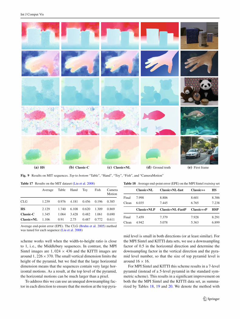
Fig. 9 Results on MIT sequences. Top to bottom “Table”, “Hand”, “Toy”, “Fish”, and “CameraMotion”

Table 17 Results on the MIT dataset (Liu et al. 2008)

Average Table Hand Toy Fish CameraMotion

CLG 1.239 0.976 4.181 0.456 0.196 0.385

HS 2.129 1.740 6.108 0.620 1.309 0.869

Classic-C 1.345 1.064 3.428 0.482 1.061 0.690

Classic+NL 1.106 0.91 2.75 0.487 0.772 0.611

Average end-point error (EPE). The CLG (Bruhn et al. 2005) methodwas tuned for each sequence (Liu et al. 2008)

scheme works well when the width-to-height ratio is closeto 1, i. e., the Middlebury sequences. In contrast, the MPISintel images are 1, 024 × 436 and the KITTI images arearound 1, 226×370. The small vertical dimension limits theheight of the pyramid, but we find that the large horizontaldimension means that the sequences contain very large hor-izontal motions. As a result, at the top level of the pyramid,the horizontal motions can be much larger than a pixel.

To address this we can use an unequal downsampling fac-tor in each direction to ensure that the motion at the top pyra-

Table 18 Average end-point error (EPE) on the MPI Sintel training set

Classic+NL Classic+NL-fast Classic++ HS

Final 7.998 8.806 8.601 8.386

Clean 6.035 7.445 6.765 7.238

Classic+NLP Classic+NL-FastP Classic++P HSP

Final 7.459 7.379 7.928 8.291

Clean 4.942 5.078 5.363 6.899

mid level is small in both directions (or at least similar). Forthe MPI Sintel and KITTI data sets, we use a downsamplingfactor of 0.5 in the horizontal direction and determine thedownsampling factor in the vertical direction and the pyra-mid level number, so that the size of top pyramid level isaround 16 × 16.

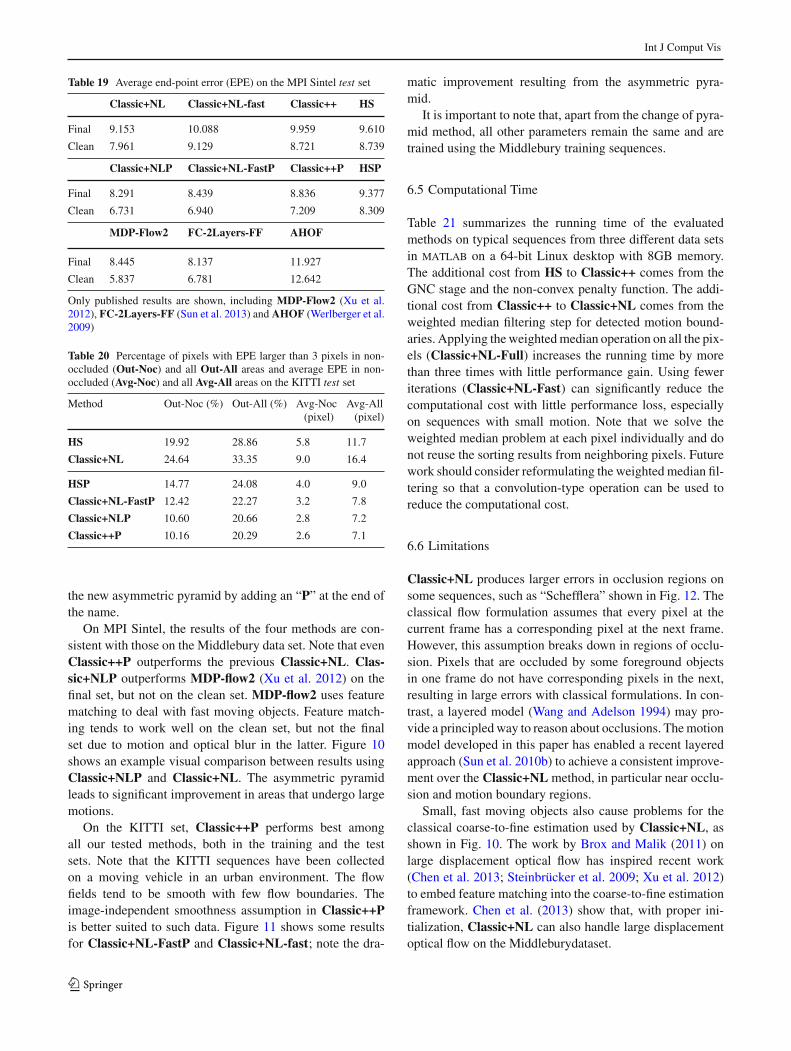
For MPI Sintel and KITTI this scheme results in a 7-levelpyramid (instead of a 5-level pyramid in the standard sym-metric scheme). This results in a significant improvement onboth the the MPI Sintel and the KITTI data set, as summa-rized by Tables 18, 19 and 20. We denote the method with

123

Int J Comput Vis

Table 19 Average end-point error (EPE) on the MPI Sintel test set

Classic+NL Classic+NL-fast Classic++ HS

Final 9.153 10.088 9.959 9.610

Clean 7.961 9.129 8.721 8.739

Classic+NLP Classic+NL-FastP Classic++P HSP

Final 8.291 8.439 8.836 9.377

Clean 6.731 6.940 7.209 8.309

MDP-Flow2 FC-2Layers-FF AHOF

Final 8.445 8.137 11.927

Clean 5.837 6.781 12.642

Only published results are shown, including MDP-Flow2 (Xu et al.2012), FC-2Layers-FF (Sun et al. 2013) and AHOF (Werlberger et al.2009)

Table 20 Percentage of pixels with EPE larger than 3 pixels in non-occluded (Out-Noc) and all Out-All areas and average EPE in non-occluded (Avg-Noc) and all Avg-All areas on the KITTI test set

Method Out-Noc (%) Out-All (%) Avg-Noc(pixel)

Avg-All(pixel)

HS 19.92 28.86 5.8 11.7

Classic+NL 24.64 33.35 9.0 16.4

HSP 14.77 24.08 4.0 9.0

Classic+NL-FastP 12.42 22.27 3.2 7.8

Classic+NLP 10.60 20.66 2.8 7.2

Classic++P 10.16 20.29 2.6 7.1

the new asymmetric pyramid by adding an “P” at the end ofthe name.

On MPI Sintel, the results of the four methods are con-sistent with those on the Middlebury data set. Note that evenClassic++P outperforms the previous Classic+NL. Clas-sic+NLP outperforms MDP-flow2 (Xu et al. 2012) on thefinal set, but not on the clean set. MDP-flow2 uses featurematching to deal with fast moving objects. Feature match-ing tends to work well on the clean set, but not the finalset due to motion and optical blur in the latter. Figure 10shows an example visual comparison between results usingClassic+NLP and Classic+NL. The asymmetric pyramidleads to significant improvement in areas that undergo largemotions.

On the KITTI set, Classic++P performs best amongall our tested methods, both in the training and the testsets. Note that the KITTI sequences have been collectedon a moving vehicle in an urban environment. The flowfields tend to be smooth with few flow boundaries. Theimage-independent smoothness assumption in Classic++Pis better suited to such data. Figure 11 shows some resultsfor Classic+NL-FastP and Classic+NL-fast; note the dra-

matic improvement resulting from the asymmetric pyra-mid.

It is important to note that, apart from the change of pyra-mid method, all other parameters remain the same and aretrained using the Middlebury training sequences.

6.5 Computational Time

Table 21 summarizes the running time of the evaluatedmethods on typical sequences from three different data setsin matlab on a 64-bit Linux desktop with 8GB memory.The additional cost from HS to Classic++ comes from theGNC stage and the non-convex penalty function. The addi-tional cost from Classic++ to Classic+NL comes from theweighted median filtering step for detected motion bound-aries. Applying the weighted median operation on all the pix-els (Classic+NL-Full) increases the running time by morethan three times with little performance gain. Using feweriterations (Classic+NL-Fast) can significantly reduce thecomputational cost with little performance loss, especiallyon sequences with small motion. Note that we solve theweighted median problem at each pixel individually and donot reuse the sorting results from neighboring pixels. Futurework should consider reformulating the weighted median fil-tering so that a convolution-type operation can be used toreduce the computational cost.

6.6 Limitations

Classic+NL produces larger errors in occlusion regions onsome sequences, such as “Schefflera” shown in Fig. 12. Theclassical flow formulation assumes that every pixel at thecurrent frame has a corresponding pixel at the next frame.However, this assumption breaks down in regions of occlu-sion. Pixels that are occluded by some foreground objectsin one frame do not have corresponding pixels in the next,resulting in large errors with classical formulations. In con-trast, a layered model (Wang and Adelson 1994) may pro-vide a principled way to reason about occlusions. The motionmodel developed in this paper has enabled a recent layeredapproach (Sun et al. 2010b) to achieve a consistent improve-ment over the Classic+NL method, in particular near occlu-sion and motion boundary regions.

Small, fast moving objects also cause problems for theclassical coarse-to-fine estimation used by Classic+NL, asshown in Fig. 10. The work by Brox and Malik (2011) onlarge displacement optical flow has inspired recent work(Chen et al. 2013; Steinbrücker et al. 2009; Xu et al. 2012)to embed feature matching into the coarse-to-fine estimationframework. Chen et al. (2013) show that, with proper ini-tialization, Classic+NL can also handle large displacementoptical flow on the Middleburydataset.

123

Int J Comput Vis

Fig. 10 Example results on MPI Sintel dataset. From top to bottom:first frame, second frame, results by Classic+NL (5-level), results byClassic+NLP (7-level), and ground truth. The asymmetric pyramidleads to a significant improvements in large regions undergoing largemotion (head of the dragon on the left and background on the right).

EPE results: “temple2” (left), 18.04 by Classic+NL (5-level) and 12.92by Classic+NLP (7-level); “cave2” (right), 52.208 by Classic+NL (5-level) and 26.565 by Classic+NLP (7-level). Note that the estimatedmotion for fast-moving objects still contains large errors

123

Int J Comput Vis

Fig. 11 Example results on the KITTI dataset. From top to bottom: firstframe, second frame, results by Classic+NL-fast (5-level), results byClassic+NL-FastP (7-level), and ground truth for the non-occluded fea-ture points. EPE results in non-occluded sparse feature points: “000002”

(left), 12.124 by Classic+NL-fast (5-level) and 2.444 by Classic+NL-FastP (7-level); “000030” (right), 20.554 by Classic+NL-fast (5-level)and 0.615 by Classic+NL-FastP (7-level)

Table 21 Running time (in minutes) for computing one optical flowfield from an image pair from different benchmark datasets using differ-ent methods in matlab on a 64-bit Linux desktop with 8GB memory

Middlebury MPI Sintel KITTI

HS 1.62 1.8 2.56

Classic++ 5.83 7.2 8.48

Classic+NL 9.81 14 14.78

C+NL-fast 1.8 2.5 2.89

C+NL-full 26.7 29 42

Used sequences: 640×480 Urban from Middlebury, 1024×436 alley_1from MPI Sintel, and 1226 × 370 training image 0 from KITTI

7 Conclusions

When implemented using modern practices, classical opti-cal flow formulations can produce fairly competitive results

(a) First frame (b) Ground truth (c) Estimated flow field

Fig. 12 Occlusions are not explicitly modeled by Classic+NL and maycause problems in the estimated flow field. Dark pixels in the groundtruth indicate occlusions

on existing datasets. To understand the techniques thathelp such basic formulations work well, we quantitativelystudied various aspects of flow approaches from the lit-

123

Int J Comput Vis

erature, including their implementation details. Amongthe best practices, we found that using median filteringto denoise the flow after every warping step is key toimproving accuracy, but that this increases the energy ofthe final result. Exploiting connections between medianfiltering and L1-based denoising, we showed that algo-rithms relying on a median filtering step are approxi-mately optimizing a different objective that regularizes theflow field over a large spatial neighborhood. Understand-ing this enables us to design and optimize improved mod-els that weight the neighbors adaptively in an extendedimage region. The Matlab code is publicly availableat http://www.cs.brown.edu/people/dqsun; last accessed 24July 2013.

There has been much debate about whether methodsthat perform well on Middlebury will generalize to othersequences. Here we tuned the parameters of the method onthe Middlebury training set and tested on Middlebury, MITHAMA, MPI Sintel, and KITTI. The conclusions on the Mid-dlebury dataset are consistent with those on the MIT HAMAdataset. The one significant difference we found betweenMiddlebury and the MPI Sintel and KITTI datasets wasthe aspect ratio of the images. This allowed us to make achange to the method by introducing a novel asymmetricimage pyramid that downsamples more rapidly in the hor-izontal direction than the vertical direction. With only thischange we found that our conclusions on Middlebury holdfor MPI Sintel as well. The KITTI data set is somewhatdifferent in nature and seems to favor methods with morespatial smoothing. As a result, the image-independent Clas-sic++, which produces more smooth flow fields, performsslightly better than the image-dependent Classic+NL, withits sharp boundaries. It is open whether these conclusionswill hold for data taken under totally different conditions,such as medical images. While the results on Middleburygeneralize surprisingly well, we suspect that training theparameters for a specific dataset will improve results fur-ther.

Acknowledgments DS and MJB were supported by a gift from IntelCorp. and NSF CRCNS award IIS-0904875. DS was also supported byKitware, Nvidia, Google, and the Intel Science and Technology Centerfor Visual Computing. We thank the CVPR and IJCV reviewers forconstructive comments, especially the connection between our original“area” term and non-local regularization and test on additional datasets,P. Yadollahpour for his early work on implementing the HS method, S.Zuffi for suggesting the color version of the non-local term, J. Wulff forrunning some experiments, T. Brox, A. Wedel, and M. Werlberger forclarifying details about their papers, and D. Scharstein for maintainingthe online optical flow benchmark.

Open Access This article is distributed under the terms of the CreativeCommons Attribution License which permits any use, distribution, andreproduction in any medium, provided the original author(s) and thesource are credited.

References

Adato, Y., Zickler, T., & Ben-Shahar, O. (2011). A polar representationof motion and implications for optical flow. In IEEE InternationalConference on Computer Vision and Pattern Recognition (pp. 1145–1152).

Adelson, E. H., Anderson, C. H., Bergen, J. R., Burt, P. J., & Ogden,J. M. (1984). Pyramid methods in image processing. RCA Engineer,29(6), 33–41.

Álvarez, L., Castaño-Moraga, C. A., García, M., Krissian, K., Mazorra,L., Salgado,A. & Sánchez, J. (2007). Symmetric optical flow. EURO-CAST (pp. 676–683). Springer, Berlin.

Bab-Hadiashar, A., & Suter, D. (1998). Robust optic flow computation.International Journal of Computer Vision, 29(1), 59–77.

Baker, S., Scharstein, D., Lewis, J., Roth, S., Black, M. J. & Szeliski,R. (2007). A database and evaluation methodology for optical flow.In IEEE International Conference on Computer Vision.

Barron, J., Fleet, D., & Beauchemin, S. (1994). Performance of opticalflow techniques. International Journal of Computer Vision, 12(1),43–77.

Bergen, J., Anandan, P., Hanna, K., & Hingorani, R. (1992). Hierar-chical model-based motion estimation. In European Conference onComputer Vision (Vol. 588, pp. 237–252).

Black, M., & Jepson, A. (1996). Estimating optical-flow in segmentedimages using variable-order parametric models with local deforma-tions. IEEE Transaction on Pattern Analysis Machine Intelligence,18(10), 972–986.

Black, M. J., & Anandan, P. (1996). The robust estimation of multiplemotions: Parametric and piecewise-smooth flow fields. ComputerVision and Image Understanding, 63, 75–104.

Blake, A., & Zisserman, A. (1987). Visual reconstruction. Cambridge,MA: The MIT Press.

Brox, T., Bruhn, A., Papenberg, N. & Weickert, J. (2004). High accuracyoptical flow estimation based on a theory for warping. In EuropeanConference on Computer Vision (Vol. IV, pp. 25–36).

Brox, T., & Malik, J. (2011). Large displacement optical flow: Descrip-tor matching in variational motion estimation. IEEE Transaction onPattern Analysis Machine Intelligence, 33(3), 500–513.

Bruhn, A., Weickert, J. (2005). Towards ultimate motion estimation:Combining highest accuracy with real-time performance. In IEEEInternational Conference on Computer Vision (Vol. 1, pp. 749–755).

Bruhn, A., Weickert, J., & Schnörr, C. (2005). Lucas/Kanade meetsHorn/Schunck: Combining local and global optic flow methods.International Journal of Computer Vision, 61(3), 211–231.

Buades, A., Coll, B., & Morel, J. (2005). A non-local algorithm forimage denoising. In IEEE International Conference on ComputerVision and Pattern Recognition (Vol. 2, pp. 60–65).

Burt, P. J., Yen, C. & Xu, X. (1982). Local correlation measures formotion analysis: A comparative study. In Proceedings of IEEE Pat-tern Recognition and Image Processing (pp. 269–274).

Butler, D. J., Wulff, J., Stanley, G. B., & Black, M. J. (2012). A natu-ralistic open source movie for optical flow evaluation. In EuropeanConference on Computer Vision (Vol. IV, pp. 611–625).

Chen, Z., Jin, H., Lin, Z., Cohen, S. & Wu, Y. (2013). Large displace-ment optical flow from nearest neighbor fields. In IEEE InternationalConference on Computer Vision and Pattern Recognition.

Chen, Z., Wu, Y., & Wang, J. (2012). Decomposing and regularizingsparse/non-sparse components for motion field estimation. In IEEEInternational Conference on Computer Vision and Pattern Recogni-tion (pp. 1176–1183).

Geiger, A., Lenz, P. & Urtasun, R. (2012). Are we ready for autonomousdriving? The KITTI vision benchmark suite. In IEEE InternationalConference on Computer Vision and Pattern Recognition (pp. 3354–3361).

123

Int J Comput Vis

Geman, S., & Geman, D. (1984). Stochastic relaxation, Gibbs distribu-tions, and the Bayesian restoration of images. IEEE Transaction onPattern Analysis Machine Intelligence, 6(6), 721–741.

Gilboa, G., & Osher, S. (2008). Nonlocal operators with applicationsto image processing. SIAM Multiscale Modeling and Simulation, 7,1005–1028.

Glaer, F., Reynolds, G., & Anandan, P. (1983). Scene matching by hier-archical correlation. In IEEE International Conference on ComputerVision and Pattern Recognition (pp. 432–441).

Horn, B. (1986). Robot vision. Cambridge, MA: MIT Press.Horn, B., & Schunck, B. (1981). Determining optical flow. Artificial

Intelligence, 16(1–3), 185–203.Hsiao, I., Rangarajan, A., & Gindi, G. (2003). A new convex edge-

preserving median prior with applications to tomography. IEEETransactions on Medical Imaging, 22(5), 580–585.

Humayun, A., Mac Aodha, O. & Brostow, G. J. (2011). Learning to findocclusion regions. In IEEE International Conference on ComputerVision and, Pattern Recognition (pp. 2161–2168).

Jia, K., Wang, X. & Tang, X. (2011). Optical flow estimation usinglearned sparse model. In IEEE International Conference on Com-puter Vision (pp. 2391–2398).

Keys, R. G. (1981). Cubic convolution interpolation for digital imageprocessing. IEEE Transactions on Acoustics, Speech and SignalProcessing, 29(6), 1153–1160.

Krähenbühl, P., & Koltun, V. (2012). Efficient nonlocal regularizationfor optical flow. In European Conference on Computer Vision (Vol.I, pp. 356–369).

Lei, C., Yang, Y.-H. (2009). Optical flow estimation on coarse-to-fineregion-trees using discrete optimization. In IEEE International Con-ference on Computer Vision (pp. 1562–1569).

Lempitsky, V., Roth, S., Rother, C. (2008). FusionFlow: Discrete-continuous optimization for optical flow estimation. In IEEE Inter-national Conference on Computer Vision and, Pattern Recognition.

Lempitsky, V., Rother, C., Roth, S., & Blake, A. (2010). Fusion movesfor Markov random field optimization. IEEE Transaction on PatternAnalysis Machine Intelligence, 32(8), 1392–1405.

Li, Y., & Osher, S. (2009). A new median formula with applications toPDE based denoising. Communications in Mathematical Sciences,7(3), 741–753.

Lin, D., & Fisher, J. (2012). Low level vision via switchable Markovrandom fields. In IEEE International Conference on Computer Visionand Pattern Recognition (pp. 2432–2439).

Liu, C., Freeman, W. T., Adelson, E. H., & Weiss, Y. (2008). Human-assisted motion annotation. In IEEE International Conference onComputer Vision and Pattern Recognition.

Lucas, B., & Kanade, T. (1981). An iterative image registration tech-nique with an application to stereo vision. In International JointConferences on Artificial Intelligence (pp. 674–679).

Mac Aodha, O., Brostow, G. J., & Pollefeys, M. (2010). Segmentingvideo into classes of algorithm-suitability. In IEEE InternationalConference on Computer Vision and Pattern Recognition (pp. 1778–1785).

Marr, D. (1982). Vision: A computational investigation into the humanrepresentation and processing of visual information. New York:W.H. Freeman.

Nagel, H.-H., & Enkelmann, W. (1986). An investigation of smooth-ness constraints for the estimation of displacement vector fields fromimage sequences. IEEE Transaction on Pattern Analysis MachineIntelligence, 8(5), 565–593.

Nikolova, M. (2007). Model distortions in Bayesian MAP reconstruc-tion. AIMS Journal on Inverse Problems and Imaging, 1, 399–422.

Nir, T., Bruckstein, A. M., & Kimmel, R. (2008). Over-parameterizedvariational optical flow. International Journal of Computer Vision,76(2), 205–216.

Niu, Y., Feng, W., & Liu, F. (2012). Enabling warping on stereoscopicimages. ACM Transactions on Graphics, 31(6), 183.

Press, W. H., Vetterling, W. T., Teukolsky, S. A., & Flannery, B. P.(2002). Numerical recipes in C++: The art of scientific computing.New York: Cambridge University Press.

Ren, X. (2008). Local grouping for optical flow. In IEEE InternationalConference on Computer Vision and Pattern Recognition.

Rudin, L. I., Osher, S., & Fatemi, E. (1992). Nonlinear total variationbased noise removal algorithms. Physica D: Nonlinear Phenomena,60(1–4), 259–268.

Sand, P., & Teller, S. (2008). Particle video: Long-range motion esti-mation using point trajectories. International Journal of ComputerVision, 80(1), 72–91.

Schmidt, U., Gao, Q., & Roth, S. (2010). A generative perspectiveon MRFs in low-level vision. In IEEE International Conference onComputer Vision and Pattern Recognition (pp. 1751–1758).

Shulman, D. & Herve, J.-Y. (1989). Regularization of discontinuousflow fields. In Workshop on Visual Motion (pp. 81–86).

Steinbrücker, F., Pock, T. & Cremers, D. (2009). Large displacementoptical flow computation without warping. In IEEE InternationalConference on Computer Vision (pp. 1609–1614).

Sun, D., Roth, S., & Black, M. J. (2010a). Secrets of optical flow esti-mation and their principles. In IEEE International Conference onComputer Vision and Pattern Recognition (pp. 2432–2439).

Sun, D., Roth, S., Lewis, J. P. & Black, M. J. (2008). Learning opticalflow. In European Conference on Computer Vision (Vol. III, pp. 83–97).

Sun, D., Sudderth, E. B., & Black, M. J. (2010b). Layered image motionwith explicit occlusions, temporal consistency, and depth ordering.In Advances in Neural Information Processing Systems (pp. 2226–2234). Cambridge, MA: MIT Press

Sun, D., Sudderth, E. B., & Black, M. J. (2012). Layered segmentationand optical flow estimation over time. In IEEE International Confer-ence on Computer Vision and Pattern Recognition (pp. 1768–1775).

Sun, D., Wulff, J., Sudderth, E. B., Pfister, H., & Black, M. J. (2013). Afully-connected layered model of foreground and background flow.In IEEE International Conference on Computer Vision and PatternRecognition (pp. 1768–1775).

Szeliski, R. (2010). Computer vision: Algorithms and applications. NewYork: Springer.

Vaudrey, T. & Klette, R. (2009). Residual images remove illuminationartifacts! In Pattern Recognition (Proceedings of DAGM) (pp. 472–481). Berlin: Springer.

Wang, J. Y. A., & Adelson, E. H. (1994). Representing moving imageswith layers. IEEE Transactions on Image Processing, 3(5), 625–638.

Wedel, A., Pock, T., Braun, J., Franke, U. & Cremers, D. (2008a).Duality TV-L1 flow with fundamental matrix prior. In Image andVision Computing New Zealand.

Wedel, A., Pock, T., Zach, C., Cremers, D., & Bischof, H. (2008b).An improved algorithm for TV-L1 optical flow. In Dagstuhl MotionWorkshop (pp. 23–45).

Wedel, A., Pock, T. & Cremers, D. (2009). Structure- and motion-adaptive regularization for high accuracy optic flow. In IEEE Inter-national Conference on Computer Vision (pp. 1663–1668).

Werlberger, M., Pock, T., & Bischof, H. (2010). Motion estimationwith non-local total variation regularization. In IEEE InternationalConference on Computer Vision and Pattern Recognition (pp. 2464–2471).

Werlberger, M., Trobin, W., Pock, T., Wedel, A., Cremers, D. & Bischof,H. (2009). Anisotropic Huber-L1 optical flow. In Proceedings of theBritish Machine Vision Conference (pp. 108.1–108.11).

Wilcoxon, F. (1945). Individual comparisons by ranking methods. Bio-metrics Bulletin, 1(6), 80–83.

Xiao, J., Cheng, H., Sawhney, H., Rao, C., & Isnardi, M. (2006).Bilateral filtering-based optical flow estimation with occlusiondetection. In European Conference on Computer Vision (Vol. I,pp. 211–224).

123

Int J Comput Vis

Xu, L., Chen, J., & Jia, J. (2008). A segmentation based variationalmodel for accurate optical flow estimation. In European Conferenceon Computer Vision (Vol. I, pp. 671–684).

Xu, L., Jia, J., & Matsushita, Y. (2012). Motion detail preserving opti-cal flow estimation. IEEE Transaction on Pattern Analysis MachineIntelligence, 34(9), 1744–1757.

Yoon, K., & Kweon, I. (2006). Adaptive support-weight approachfor correspondence search. IEEE Transaction on Pattern AnalysisMachine Intelligence, 28(4), 650–656.

Zach, C., Pock, T. & Bischof, H. (2007). A duality based approach forrealtime TV-L1 optical flow. In Pattern Recognition (Proceedings ofDAGM) (pp. 214–223).

Zimmer, H., Bruhn, A., & Weickert, J. (2011). Optic flow in harmony.International Journal of Computer Vision, 93(3), 368–388.

Zimmer, H., Bruhn, A., Weickert, J., Valgaerts, L., Salgado, A., Rosen-hahn, B. & Seidel, H.-P. (2009). Complementary optic flow. InEnergy Minimization Methods in Computer Vision and PatternRecognition (pp. 207–220).

Zitnick, C., Jojic, N., & Kang, S. B. (2005). Consistent segmentationfor optical flow estimation. In IEEE International Conference onComputer Vision (Vol. 2, pp. 1308–1315).

123