A QUANTIFIER ELIMINATION FOR THE

THEORY OF P -ADIC NUMBERS

Lavinia Egidi

Abstract. This paper presents a detailed analysis of a quantifier elimi-nation algorithm for the first order theory of p-adic numbers based on ap-adic analogue of the cylindric algebraic decomposition. It is believedthat such method should lead to an elementary upper bound for the the-ory. The present paper gives strong arguments against this conjectureand offers a basis for further speculation.

Key words. Complexity; theory of p-adic numbers; cylindric algebraicdecomposition.

Subject classifications. 68Q25

1. Introduction

The first order theory of p-adic numbers is, for each fixed prime p, the firstorder theory of henselian fields of characteristic 0 that have finite residue classfield, a Z-group as valuation group, and in which the valuation of p is one.A lower bound for the decision problem in this theory has been known for along time; it is the same one that holds for Presburger arithmetic (since thelatter is interpreted in the theory of p-adics numbers), i.e., doubly exponentialalternating time with a linear number of alternations. As for the upper bound,the best algorithm known so far is due to Cohen [6] and it is primitive recursivebut not elementary. It is a quantifier elimination process in which the formulaanalyzed is expanded in a dramatic (double exponential?) way each time aquantifier is eliminated.

The problem of a similar explosion was faced before, in the different contextof the first order theory of the reals Th(R). Consider, for instance, Cohen’s real

2

counterpart ([6]) of his own algorithm for Th(Qp). Like the latter, it treats thequantified variables one at a time and suffers of an exponential growth at eachstep of the recursion. The solution proposed in the real case by Collins [7] isa way of eliminating all the quantifiers at the same time, through exploitationof geometrical properties of polynomials and their roots.

Since there are interesting analogies between the real field and the p-adicfield Qp (see [12]) it is reasonable to expect that an elementary algorithm couldbe obtained by using on the p-adics Collins’ method. Macintyre [12] conjecturedthat the complexity of Th(Qp) be the same as that of Presburger arithmetic(since the former interprets the latter), and he suggested [13] that a fast algo-rithm should be based on an analogue of Collins’ quantifier elimination. Indeed,it is by exploiting similar ideas that Brown [5] proved interesting complexitybounds about transfer principles involving Qp. Scowcroft and Van den Dries[14] point out that the essential algebra needed for tailoring the method to thep-adic case is provided by Denef’s study [8] of a cylindric algebraic decomposi-tion for Qp, and point out the complexity aspect of the problem.

Nevertheless, note that the mentioned analogies between p-adics and realscannot be pushed too far. A deep difference between the topological propertiesof the two fields complicates significantly the p-adic setting. The topology ofQp is totally disconnected. Because of this no analogue of Sturm’s theoremis known so far. This has serious implications on the quantifier eliminationssince they essentially come down to root isolations and related polynomialmanipulations.

A first consequence of this fact is that at present one can’t think of adaptingto the theory of Qp the algorithm due to Ben-Or, Kozen and Reif [4], whichis an alternative, more efficient decision procedure for the theory of the reals.Collins’ algorithm requires double exponential time. Ben-Or, Kozen and Reifhave proven an exponential space upper bound, but their work makes use inan essential way of Sturm sequences and Sturm’s theorem.

A second consequence is that the only technique available for treating rootsof polynomials is quite cumbersome from a complexity point of view, as will beclarified later.

The present paper studies Collins’ method, and uses Denef’s ideas in ad-dition. The whole analysis will be useful for a better understanding of thecomplexity of the theory of p-adic numbers. It leads to interesting conclusionsthat are meant to provoke some discussion on the subject.

It turns out that there is one critical point where the complexity of thealgorithm explodes and, as mentioned, the uncontrolled growth of the com-plexity seems to depend on the way that the roots of polynomials are treated.

3

Indeed this calls for a comparison with the real case for understanding whatmakes a good method for R ineffective on Qp. The point is discussed in thefinal section, but it is worth anticipating that a natural interpretation of thephenomenon leads back to the lack of some analogue of Sturm’s theorem onthe p-adics.

This suggests an investigation of the depth of the differences between p-adic and real fields. It stirs curiosity on the inherent difficulty of the treatmentof polynomials and their roots. However the question of whether the methodcould still lead to an elementary algorithm by some shortcut or ad hoc algebraicmanipulation remains open.

A full understanding of the nature and complexity of the p-adic version ofCollins’ method is a good starting point for further pursuits of answers to theabove questions.

This paper is an attempt to present the methodology clearly.The theoretical background on which the algorithm is based is described in

detail, at the same time providing a bridge between the existential characterof many proofs and a more constructive point of view.

The algorithm is organized in a modular way for understandability and easeof complexity analysis. Its structure is as close as possible to that of Collins’algorithm which makes it easier to compare the two scenarios. To obtain analgorithm of this form it was necessary to unwind the multiple recursions hiddenbehind Denef’s clean exposition, taking care not to remain entangled in themany tiny threads.

The complexity analysis is exposed in two distinct, neatly separated parts,in order to make evident how far the method is efficient and what makes it nonelementary in the end. This feature enhances the intended character of thispaper as a basis for further research in the area.

In writing about my work I have been struggling for readability yet notwanting to give up precision. The subject is itself so intricate at times thatit hasn’t been possible to avoid clumsiness. Yet I have tried to identify basicsteps and essential concepts and to build the paper around them. There arecomplex definitions that are intended to provide clean and intuitive tools forexposing the arguments. Fine detail is hidden in these structures, yet availableto the interested reader.

The paper is essentially self-contained. Some proofs that are available else-where in the literature are here simply sketched in order to provide the basis forfurther analysis without overloading the paper. Only a few have been omittedaltogether but, in such cases, precise references have been provided for them; Ibelieve that the absence of these proofs will not impair the comprehension of

4

the material presented.

Section 2 gives the main notions about p-adic fields and the theory studiedin the paper. In the subsequent sections (Sections 3 and 4) the state of the artis discussed in a progressive fashion leading to the description of the methodused in this paper. All the theoretical background is given.

Subsection 4.1 is essentially an anticipation of the proof of correctness. Itis necessary in order to introduce smoothly the reader to the algorithm.

Subsections 4.2 and 4.3 are mainly concerned with remarks on the notationbut also stress some non obvious points.

Section 5 defines the support structures mentioned above.Then the algorithm is presented, in all its details (Section 6). As described

here it works for a prenex formula only, but it could be slightly modified towork also for a general formula using the same amount of space.

The proof of correctness (Section 7) should help put together all the tilesof the puzzle.

Section 8 gives a detailed analysis of the complexity. It follows the modularorganization of the presentation of the algorithm and benefits from the supporttools defined in the previous chapters. Where possible, the proofs follow thestructure of the definitions of the objects that they analyze.

A concluding section attempts a brief comparison between the cylindricalgebraic decomposition for the reals and its p-adic counterpart.

2. The p-adic numbers and the theory

Let p denote any fixed prime number. A map that satisfies the following prop-erties

1. |x|p ≥ 0 ∧ (|x|p = 0 ↔ x = 0)2. |x · y|p = |x|p · |y|p3. |x+ y|p ≤ max(|x|p, |y|p) (ultrametric inequality)4. |p|p = 1

p

is called p-adic norm (it is a non-Archimedean norm). The completion of thefield Q of rational numbers with respect to | · |p : Q → pnn∈Z

⋃0 is the fieldof p-adic numbers Qp. Notice that this construction mimicks the constructionof the reals from Q. The p-adic norm over Qp (also denoted | · |p) is definedin the obvious way from the p-adic norm over Q and takes values in the samerange.

5

On Qp one can define the valuation, a map vp : Qp → Z⋃∞ logarithmi-

cally related to the p-adic norm. It satisfies the following properties:

1. vpx ≤ ∞∧ (vpx = ∞↔ x = 0)2. vp(x · y) = vpx+ vpy3. vp(x+ y) ≥ min(vpx, vpy)4. vpp = 1.

Qp is said to be a field with valuation. Z is the valuation group of Qp.The subdomain of Qp of p-adic integers, i.e. p-adic numbers with non-

negative valuation, is denoted Zp. The elements of Z are sometimes calledrational integers to distinguish them explicitly from the p-adic integers.

The unique maximal ideal of Zp is Mp = x ∈ Zp|vpx > 0. The quotientZp/Mp, the residue class field of Qp, is the field of p elements Fp.

Each p-adic number is uniquely determined by its valuation and its angularcomponent. For each b ∈ Qp

b = pvpb · acb

where ac : Qp → Zp takes as argument a p-adic number and yields its angularcomponent. Intuitively ac(x) = x · p−vpx.

Any p-adic number b can be written in a unique way as

b =∞∑i=s

bipi (2.1)

where s is any rational integer, and bi ∈ 1, . . . , p− 1. The expression on theright hand side of (2.1) is called p-adic expansion of b. In terms of the p-adicexpansion, the valuation of b is the least i such that bi is nonzero (in case b ∈ Z,it amounts to saying that pi is the largest power of p that divides b).

Given any pair of p-adic integers x and y, write x ≡ y mod ps for vp(x−y) ≥s. This notation induces obvious concepts of residue class and residue, moduloa power of p.

An essential tool in p-adic arithmetic is Hensel’s Lemma. It gives a sufficientcondition for the existence of a root.

Lemma 2.1. (Hensel’s Lemma) Let f(x) be a polynomial

f(x) = a0 + a1x+ . . .+ adxd

where ai ∈ Zp. Let f ′(x) be

f ′(x) = a1 + 2a2x+ . . .+ dadxd−1.

6

Let β ∈ Zp. If f(β) ≡ 0 mod p2e+1, and f ′(β) 6≡ 0 mod pe+1 for some non-negative integer e, then there exists ξ ∈ Zp such that f(ξ) = 0 and ξ ≡β mod pe+1.

The proof can be found in [10] for the case e = 1, or, e.g., in [6].

A field with valuation in which the above lemma holds is called henselian.By looking at a few more residue classes, Hensel’s Lemma can be used as a

necessary and sufficient condition for the existence of roots:

Lemma 2.2. (Existence of roots) Let f(x) and f ′(x) be as in Lemma 2.1.Assume that, for x ∈ Zp, vpf

′(x) ≤ e. Then f has a root ξ ∈ Zp if and onlyif there exists a residue modulo p2e+1, β, that satisfies Hensel’s Lemma. Theroot will be such that ξ ≡ β mod p2e+1.

Proof. The “if” part is a weak form of Hensel’s Lemma. For the “onlyif” part, consider that since the coefficients of f ′(x) are clearly p-adic integersby the assumptions on f(x), and the same holds for x by hypothesis, e mustbe non-negative. Let ξ ∈ Zp be a root of f(x). Now vpf

′(x) ≤ e, for x ∈ Zp

implies vpf′(ξ) < e+ 1; on the other hand vpf(ξ) ≥ 2e+ 1, for ξ is a zero of f .

Therefore, any β such that β ≡ ξ mod p2e+1, satisfies the hypotheses of Lemma2.1. 2

This brief introduction to Qp shows that (for each prime p) the field of p-adicnumbers is a model of the first order theory of henselian fields of characteristic0, with finite residue class field, valuation group a Z-group, and vpp = 1. Thetheory is complete and recursively axiomatizable, therefore decidable [1]-[3]; itscompleteness enables us to reason about one of its models in order to deriveresults about the whole theory. In this light we refer to it as Th(Qp). It isexpressible in a variety of languages, ranging from one with infinitely manysorts, in which the valuation is expressed by a symbol of the language (see [6]),to a language with only one sort.

The latter choice is possible because the valuation is definable in the purefield language:

Qp |= (∀x)[vpx ≥ 0 ↔ (∃y)(y2 = 1 + px2)] if p 6= 2

Qp |= (∀x)[vpx ≥ 0 ↔ (∃y)(y3 = 1 + px3)] if p 6= 3.

The axioms of Th(Qp) are those for a field with valuation (field axioms andaxioms describing properties of the valuation) together with those that state

7

that the characteristic is 0, the valuation group is a Z-group, the residue classfield is finite, Hensel’s Lemma holds and vpp = 1 (see [2]).

The theory admits quantifier elimination in a language that makes use ofthe cross-section [1]-[3]. The cross section is a map π : Z

⋃∞ → Qp actingas a right inverse of the valuation: π(x) = px. It is awkward since it introducesrather complicated definable sets.

On the other hand Th(Qp) admits quantifier elimination also in the purefield language augmented with predicates Pn, such that Pn(x) if and only if xis an n-th power [11]. The axioms that give the proper meaning to the newpredicates are thus:

(∀x)[Pn(x) ↔ (∃y)yn = x].

I work in the language with one sort and predicates Pn. My choice is motivatedby the observation that the study of complexity properties over a simpler lan-guage is more informative. Moreover, the length of a formula in the pure fieldlanguage is polynomially related to the length of the equivalent formula in atwo sorted language with a symbol for the valuation.

The logical language I use is the minimal one, containing ∧, ¬ and thequantifiers.(However, for expository reasons, I shall freely make use in the following of awider language than the one chosen.)

It should be noted that a formula of the above language can be seen as a(quantified) boolean combination of atomic formulas each stating that somepolynomial with coefficients in Z is an n-th power, for some n.(For a detailed introduction to p-adic numbers see, e.g., [10]; an interesting,broad survey is in [12]; more specifically, about quantifier elimination in valuedfields, see [15].)

3. Collins’ method for the reals

First note that any atomic formula in the language of Th(R) is a polynomialinequality, or, equivalently, it states that some polynomial is a square (in R,x ≥ 0 if and only if x is a square).

Collins’ procedure partitions the space in a finite number of sets (cells) ineach of which every polynomial that appears in the sentence to be decided hasconstant sign; then it chooses a sample point from each cell C of the partition

8

to determine the sign that each one of the polynomials involved has in C. Atthis point each existential (resp. universal) quantifier can be replaced by afinite disjunction (resp. conjunction) of the polynomial inequalities evaluatedat the sample points. In this way a block of quantifiers is eliminated in a singlestep.

A cell is a set defined recursively on the dimension of the space, bounded ateach stage by continuous realvalued algebraic functions. Its crucial property isthat the poynomials that appear in the sentence to be decided have constantsign in it. The decomposition of the space in cells can be done efficiently, asCollins shows, and, due to a nice geometry of the cells, the sample points canbe chosen in a uniform and quick way. The geometrical properties of the cellsare succintly described by the name cylindric algebraic decomposition (for shortc.a.d.) given to the cell decomposition.

4. The method for Th(Qp)

The novelty of Collins’ procedure was the idea of removing all the quantifiersin a single step. Otherwise Cohen’s algorithms are not too different in spirit.

Cohen defines a cell in Qp as a set of the form

x|x = x0 + upa, where u ∈ Zp.

Then he shows “how to cover the p-adic numbers by cells in each of which agiven polynomial behaves in a simple fashion” [6],p. 139. The “simple fashion”that Cohen refers to means essentially that the valuation of the polynomial canbe related in each cell to the valuation of one of its monomials, if necessary aftera change of variable has been performed. The following steps of the quantifierelimination are very intricated and depend on the language used (essentiallya language with infinitely many sorts, although most of them finite; it alsoincludes the cross-section).

Denef extends the notion of cell to more dimensions (here and in the fol-lowing x stands for (x1, . . . , xr), and y for (y1, . . . , ym)):

Definition 4.1. (Cell) A cell in Qrp ×Qp is a set of the form

(x, y) ∈ Qrp ×Qp|

x ∈ C ∧ vpa1(x)21vp(y − χ(x))22vpa2(x)

9

where the 2i are either ≤ or < or no condition at all, χ(x) and ai(x) are semi-algebraic functions of x, and C is a semi-algebraic subset of Qr

p. The functionχ(x) is called center of the cell.

(Note that Cohen’s definition of a cell could be rephrased as x|vp(x−x0) ≥ a.)A semi-algebraic set is a boolean combination of sets of the form

y ∈ Qmp |Pn(h(y)),

where h is a polynomial (consistently with the notion of semi-algebraic sets overthe reals which are the sets definable via polynomial inequalities). Observe thatsets of this form are the only sets that can be defined in the language chosen.

Semi-algebraic (partial) functions preserve, in some sense, semi-algebraicsets:

Definition 4.2. (Semi-algebraic functions) A function f : Qrp → Qp is

said to be semi-algebraic if for all semi-algebraic set S ⊂ Qm+1p , the set

(x, y) ∈ Qr+mp |(f(x), y) ∈ S

is also semi-algebraic.

The same notion can also be expressed in a more intuitive way:

Proposition 4.3. (Characterization) A function f : Qrp → Qp is semi-

algebraic if and only if for each polynomial h : Qm+1p → Qp and rational integer

n, there exist finitely many polynomials h∗i : Qr+mp → Qp and rational integers

mi such that the set

(x, y) ∈ Qr+mp |Pn(h(f(x), y))

can be expressed as a boolean combination of the sets

(x, y) ∈ Qr+mp |Pmi

(h∗i (x, y)).

This result follows by combining explicitly the definition of semi-algebraic func-tions with the notion of semi-algebraic set. The characterization will be usefullater; it amounts to saying that, although in general a semi-algebraic functionf is not a polynomial, yet any semi-algebraic condition on it (i.e. a condi-tion stating that a polynomial form in f is an n-th power for some n) can betranslated to another one involving only polynomials.

Denef shows that a decomposition of the r + 1-dimensional space in thespirit of Collins’ c.a.d. is definable:

10

Theorem 4.4. (Denef [8]) Let fi(x, y), for i = 1, . . . ,m, be polynomials iny with coefficients which are semi-algebraic functions of x. Let n ∈ N, n > 0,be fixed. Then there exists a finite partition of Qr

p×Qp into cells A, such thateach such cell A has a center χ(x) such that for all (x, y) ∈ A we have

fi(x, t) = ui(x, t)nhi(x)(t− χ(x))νi , for i = 1, . . . , r,

with vpui(x, y) = 0, hi(x) a semi-algebraic function of x , and νi ∈ N.

The decomposition is built in a recursive fashion as in the real case. The“boundaries” of the cells are semi-algebraic functions; the distance of this def-inition from Collins’ one is non-trivial. The difficulty that arises is better seenby a reference to the characterization of semi-algebraic functions. That charac-terization states that any semi-algebraic condition on a semi-algebraic functioncan be expressed using only polynomials and predicates Pn; it doesn’t say any-thing about how the simpler expression is to be obtained. Since our target is aprocedure, we need something constructive rather than existential.

An analysis of Denef’s decomposition reveals that, starting out with a poly-nomial, only specific functions will have to be considered. I have called thesefunctions constructive semi-algebraic to stress the fact that a witness of theirsemi-algebraic character can be computed.

Definition 4.5. (Constructive semi-algebraic functions) The set ofconstructive semi-algebraic functions is the smallest set C of functions such that:

1. +, −, × and ÷ belong to C.

2. Let g(x, t) be a polynomial in t whose coefficients are functions of xbelonging to C and taking values in Zp; let D, a semi-algebraic subset ofQrp, and e ∈ N be such that, for all x ∈ D and t ∈ Zp,

vpg′(x, t) ≤ e

(here and in the following I use the notation g′(x, t) to denote ∂∂tg(x, t)).

Let h be such thatvpg(x, h) ≥ 2e+ 1

for all x ∈ D. Then the “root-function” ξ : D → Zp such that

g(x, ξ(x)) = 0 and vp(ξ(x)− h) ≥ e+ 1

is in C.

11

3. Let ψ(x) : D → Qp be in C, where D is a semi-algebraic subset of of Qrp.

Let k ∈ N, k ≥ 2; assume that ψ(x) 6= 0 for x ∈ D, that for some svpψ(x) ≡ s mod k and that for some ρ, ψ(x) = ρ ·(nonzero N -th power),

with N = p2vpk(p− 1). Let ψ1(x) = ψ(x)ρpvpρ−s.

Then the “θ-function” θ : D → Qp such that, for all x ∈ D,

θ(x)k = ψ1(x) ∧ PN1(θ(x)),

with N1 = pvpk(p− 1), belongs to C.

4. C is closed under composition.

The class C is well defined: the existence and uniqueness of root functionsis guaranteed by Hensel’s Lemma; for θ-functions see [8], Lemma 2.4. It ismoreover the required class:

Lemma 4.6. (Constructivity) The functions in C are semi-algebraic.Moreover, for each f ∈ C, f : Qr

p → Qp, there exists a procedure to compute,given any polynomial h : Qm+1

p → Qp and rational integer n, the polynomialsh∗i and the integers mi of Proposition 4.3.

The lemma is proven by actually showing the mentioned procedure, a lengthyand very complex one. It is the same as described in [8], Lemmas 2.3 and 2.4.Although the proof is not explicitly presented here, the definition of csa-treesin Section 5 can be viewed as a (quite extended) sketch of it. For further detailsthe reader is referred to the mentioned lemmas in [8].

The constructive semi-algebraic functions are actually either polynomialsor zeroes of polynomials.

With the new “boundary”-functions, the p-adic cells have geometrical prop-erties that are in some sense analogous to those of the cells defined by Collins[7], but still play a different role in the decision procedure. In each cell of thedecomposition for the reals, each one of the polynomials at issue has constantsign. In the p-adic setting the corresponding condition is not automaticallyverified.

Saying that a polynomial has constant sign in a cell amounts (in the reals)to saying that it is a square in each point of the cell, or its opposite is. In otherwords, either the polynomial is in the same coset of the squares as 1, or it isin the same coset as −1. In the p-adic case, we must look in general at n-thpowers, not only squares; it can be proven, though, that for each n there is afinite number of different cosets of the n-th powers (Lemma 8.1). Requiringthat a polynomial have constant sign is equivalent in the p-adic setting to the

12

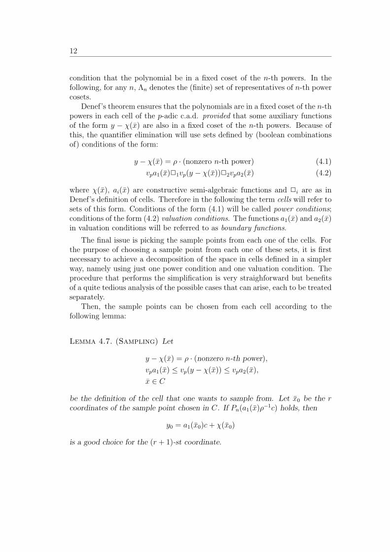
condition that the polynomial be in a fixed coset of the n-th powers. In thefollowing, for any n, Λn denotes the (finite) set of representatives of n-th powercosets.

Denef’s theorem ensures that the polynomials are in a fixed coset of the n-thpowers in each cell of the p-adic c.a.d. provided that some auxiliary functionsof the form y − χ(x) are also in a fixed coset of the n-th powers. Because ofthis, the quantifier elimination will use sets defined by (boolean combinationsof) conditions of the form:

y − χ(x) = ρ · (nonzero n-th power) (4.1)

vpa1(x)21vp(y − χ(x))22vpa2(x) (4.2)

where χ(x), ai(x) are constructive semi-algebraic functions and 2i are as inDenef’s definition of cells. Therefore in the following the term cells will refer tosets of this form. Conditions of the form (4.1) will be called power conditions;conditions of the form (4.2) valuation conditions. The functions a1(x) and a2(x)in valuation conditions will be referred to as boundary functions.

The final issue is picking the sample points from each one of the cells. Forthe purpose of choosing a sample point from each one of these sets, it is firstnecessary to achieve a decomposition of the space in cells defined in a simplerway, namely using just one power condition and one valuation condition. Theprocedure that performs the simplification is very straighforward but benefitsof a quite tedious analysis of the possible cases that can arise, each to be treatedseparately.

Then, the sample points can be chosen from each cell according to thefollowing lemma:

Lemma 4.7. (Sampling) Let

y − χ(x) = ρ · (nonzero n-th power),

vpa1(x) ≤ vp(y − χ(x)) ≤ vpa2(x),

x ∈ C

be the definition of the cell that one wants to sample from. Let x0 be the rcoordinates of the sample point chosen in C. If Pn(a1(x)ρ

−1c) holds, then

y0 = a1(x0)c+ χ(x0)

is a good choice for the (r + 1)-st coordinate.

13

This lemma is based on the ideas in the quantifier elimination in the finalsection of [8]. The procedure is slightly more complex than this to take carealso of cells in which the valuation is not bounded from below.

The geometry of the decomposition is analogous (modulo topological differ-ences) to that of Collins’ c.a.d., so that the choice of the sample points is justas straightforward. All the quantifiers can be removed at the same time:

Theorem 4.8. (Quantifier Elimination) Consider the sentence

(Q1x1) . . . (Qrxr)(Qr+1xr+1)φ(x1, . . . , xr, xr+1), (4.3)

where Qj ∈ ∃,∀, for j = 1, . . . , r + 1, and φ is a quantifier free booleancombination of atomic formulae. There exists a finite partition of Qr+1

p in cellsCi, such that, if (β1,i, . . . , βr+1,i) is the sample point chosen from Ci accordingto the Sampling Lemma, the sentence (4.3) is equivalent in the theory to

(B1)i . . . (Br)i(Br+1)iφ(β1,i, . . . , βr,i, βr+1,i),

where i ranges over all the subscripts of the cells and, for j = 1, . . . , r + 1,(Bj) =

∨if Qj = ∃, and (Bj) =

∧if Qj = ∀.

4.1. The decomposition. At the (r + 1)-st stage, a decomposition of the(r + 1)-st dimension of the space with respect to a set of conditions has to becarried out. Let

f(x, y) = ρ · (nonzero n-th power)

be one of these conditions. The polynomial appearing in it is viewed as anunivariate polynomial in the (r + 1)-st variable with coefficients that are con-structive semialgebraic functions of x:

f(x, y) = a0(x) + a1(x)y + . . .+ ad(x)yd. (4.4)

The coefficients are regarded as black boxes, except that in order for thedecomposition to be properly carried out it is assumed that at the precedingstage conditions on the coefficients and certain other appropriate functions(that will be mentioned later as they appear) have been treated. Moreover,the space must have been already decomposed in cells in each one of which thepartial derivative

f ′(x, y) = a1(x) + 2a2(x)y + . . .+ dad(x)yd−1

14

is in a fixed coset of the n-th powers. This implies an inner recursion on thedegree of f , and the decomposition relative to f is built over a decompositionrelative to f ′. Since while treating f ′ a change of variable might have beencarried out (see later for the reason why this is so), the coefficients of f are ingeneral not polynomials but more general constructive semialgebraic functions.

A second assumption on the decomposition of the r-th dimensional space isthat it has been split in cells in each one of which every coefficient of f eithernever vanishes or is always zero (notice that, for each γ ∈ Qp, γ = 0 if andonly if P2(pγ

2)). Afterwards the polynomial might not have monomials of eachdegree in y, but it is important that one takes here (4.4) as a general form forthe polynomial. It must be stressed, though, that the monomials which appearat all never vanish.

Recall that the goal is writing f as

f(x, y) = u(x, y)nh(x)(y − χ(x))ν (4.5)

where vpu(x, y) = 0, h(x) is a constructive semi-algebraic function and ν is apositive integer. Therefore if h(x) and y − χ(x) are n-th powers, so is f . Weare assuming that the required functions of x have already been dealt with,and therefore the above condition on h(x) is met. The one on y − χ(x) is oneof the conditions defining the (r + 1)-st dimension of the cell.

A fact used times and again in the process of writing f in the form (4.5) is:

Lemma 4.9. (n-th Power Residue) For any n ∈ N, there exists a rationalinteger λ for which any p-adic integer u such that u ≡ 1 (mod pλ) is an n-thpower. Namely, if v(n) = m, then λ = 2m+ 1.

The proof is obtained by direct inspection of the p-adic expansion of an n-thpower. It holds only for p-adic integers because it is based on Hensel’s Lemma.The constant λ defined in it will appear very often in the following:

Notation 4.10. (λ) Let λµ = 2vpµ + 1 for each subscript µ. If no subscriptappears, n is intended: λ = λn.

If f has coefficients that take p-adic integer values, y has non-negativevaluation too and the valuation of f is bounded in a cell, then one can splitthe space so that f ’s coefficients have fixed residues modulo λ in each cell, andthat so has y in each cell. This implies that the same holds for f , and so bylemma 4.9 f is in a fixed coset of the n-th powers.

15

Notice for instance that in the cells in which there is an i0 such that

vp(ai0(x)yi0) ≤ vp(ai(x)y

i)− λ for all i 6= i0, (4.6)

f can be written as f(x, y) = u(x, y)nai0(x)yi0 since f(x,y)

ai0(x)yi0

≡ 1 mod pλ.

But f ’s coefficients and variable are not in general p-adic integers. Thesolution is to factor f into a polynomial that has the properties just mentionedtimes some function of x.

Suppose that in the cell C, y is such that vpy = vpθ(x), and i0 is such thatvp(ai0(x)y

i0) < vp(ai(x)yi) for all i 6= i0. Then

g(x, u) =f(x, y)

ai0(x)θ(x)i0

with u =y

θ(x)(4.7)

has coefficients and variable u in Zp in the cell C. The function g will betherefore referred to as the integral polynomial relative to f .

Sincevpg(x, u) = vpf(x, y)− vp(ai0(x)θ(x)

i0),

if the differencevpf(x, y)−min

ivp(ai(x)yi) (4.8)

is bounded, so is the valuation of g, and it is possible to split the space in afinite number of cells in each of which g is in a fixed coset of the n-th powers.

The first step is therefore splitting the space in cells in such a way that ineach one of them a function like the θ(x) above can be defined, and that thedifference (4.8) is bounded.

The difference (4.8) is not bounded in cells in which f has a non-zero root.By a basic fact of p-adic arithmetic, f can have a root only in those cells inwhich vpy is such that two monomials have the same valuation. Applying theproperties of the valuation, the resulting condition on y is:

vpy =1

i− jvpaj(x)

ai(x)(4.9)

for some i 6= j.For each pair (i, j) (i, j ∈ 0, . . . , d, |i−j| ≥ 2), for each s ∈ 0, . . . , i−j−1

and ρ ∈ ΛN2 for N2 = (i− j)pvp(i−j)(p− 1), define a function θij(x) as in Item

3 of Definition 4.5, with ψ(x) = aj(x)

ai(x)and k = i− j1.

1The notation θij(x) hides the dependence of the definition from s and ρ. But a moreprecise notation would have been too heavy.

16

For the pairs (i, j) such that |i − j| = 1, let θij(x) = aj(x)

ai(x). By Item 1 of

Definition 4.5, it is a semi-algebraic function if ai(x) and aj(x) are.For each pair (i, j), vpθij(x) equals the right hand side of (4.9)—see [8],

Lemma 2.4 for a proof of this. Notice that for each pair (i, j), θij = θji.Now for each (i, j), such that j > i say, and for each θij defined with s = 0,

the cells

V (ij) =

(x, y)|(x, y) ∈ D ∧ vpy = vpθij(x)∧

∧h<i

vpy ≤ vpθih(x) ∧∧h>i

vpy ≥ vpθih(x)

might contain a root.

If the (r + 1)-th dimension of the space is split according to the valuationconditions described in each item of the following enumeration, f can be writtenin the form (4.5) in each one of the resulting sets, as discussed in each casebelow.

1. For all i = 1, . . . , d, in the cells

A(i0)λ =

(x, y)|(x, y) ∈ D∧

∧j<i0

vpθi0j(x)− vpy ≥⌈

λ

i0 − j

⌉∧

∧j>i0

vpθi0j(x)− vpy ≤⌈

λ

i0 − j

⌉i0 is as in Example (4.6); the form (4.5) for f is soon attained, as shownin that example. Here Pn(ai0(x)) ∧ Pn(y) implies Pn(f(x)).

2. For i0 = 0, . . . , d, j = 0, . . . , d, j 6= i, s = 1, . . . , λ− 1, in the cells

A(i0j)s =

(x, y)|(x, y) ∈ D ∧ vpy = vpθi0j(x)−⌈

s

i0 − j

⌉∧

∧h<i0

vpy ≤ vpθi0h(x)−⌈

s

i0 − h

⌉∧∧h>i0

vpy ≥ vpθi0h(x)−⌈

s

i0 − h

⌉ai0(x)y

i0 is the (unique) monomial of minimum order.

In each one of these cells, define the integral polynomial g relative to f

as in (4.7) above (replacing θ(x) byθi0j(x)

ps ). Its coefficients bi(x) and its

17

variable u have non-negative valuation in the cells. The valuation of gitself is null.Thus in the cells

Ch1,...,hd+1 = (x, y)|∧

0≤i≤dbi(x) ≡ hi mod pλ∧u ≡ hd+1 mod pλ (4.10)

where hi ∈ 0, . . . , pλ− 1, g(x, u) has a constant power residue, and cantherefore be written as bv(x, u)n for some integer b and function v havingvaluation 0.Therefore

f(x, y) = bv(x, u)nai0(x)

(θi0j(x)

ps

)i0.

Notice that the condition defining the space decomposition in cells of theform (4.10) is ∧

0≤i≤dbi(x) has constant residue mod pλ ∧

u has constant residue mod pλ. (4.11)

3. As mentioned, in the cells V (ij) in which vpy = vpθij(x), there might bea root.

Define here the integral polynomial relative to f , gf,d. Here θij(x) mustreplace θ(x) in the definition of the form (4.7). (The subscripts indicatethat gf,d refers to f of degree d; they will be useful soon because it willbe necessary to distinguish this function from the integral polynomialrelative to f ′.)

There exists a constant ed (which depends on the degree of f) such that

vpg′f,d(x, u) ≤ ed. (4.12)

The existence of this constant is due to the fact that

g′f,d(x, u) =f ′(x, y)

ai0(x)θij(x)i0−1

,

and that it is assumed that a c.a.d. with respect to f ′ has been carriedout.

18

Indeed, writing

g′f,d(x, u) = b1(x) + 2b2(x)u+ . . .+ dbd(x)ud−1,

the difference vpg′f,d(x, u)−mini vp(ibi(x)u

i−1) equals

vpf′(x, y)−min

ivp(iai(x)y

i−1)

which, by induction hypothesis is bounded by a constant, say Const.Since

minivp(ibi(x)u

i−1) ≤ vp(i0bi0(x)ui0−1) = vpi0.

and vpi0 < ∞, vpg′f,d(x, u) ≤ max0<i≤d vpi + Const. So it remains to

determine what Const is.The algorithm is further decomposing a cell of the c.a.d. for f ′. If no twomonomials of f ′ have the same valuation in the cell then Const = 0.This is the case also in a cell where f ′ had a root since in this case achange of variable has been performed.Otherwise, consider gf,d−1(x, u) as the integral polynomial relative to f ′

(which has degree d− 1): vpgf,d−1(x, u) ≤ 2ed−1 in this cell. Since

vpgf,d−1(x, u) = vpf′(x, y)−min

ivp(iai(x)y

i−1)

in this case Const = 2ed−1.

Consider the cells

V(ij)h = (x, y))|(x, y) ∈ V (ij) ∧ u ≡ h mod p2ed+1.

(Cells with these property are defined via the request that u have constantresidue modp2ed+1.) By Hensel’s Lemma, gf,d (and therefore f) has a

unique root only in the cell (if any) V(ij)h0

such that vpgf,d(x, h0) ≥ 2ed+1.

In the cells V(ij)h where there is no root (and therefore vpgf,d(x, h) ≤

2ed), the situation is exactly the same as in the cells A(i0j)s in Item 2

above. Assuming that in the cells of the r-dimensional decompositionseach coefficient bi(x) of g has constant residue modp2ed+λ, and adding

u has constant residue mod p2ed+λ

to the conditions defining the (r + 1)-st dimension, f can be written inthe form (4.5). Here Pn(ai(x)) ∧ Pn(θij(x)) implies Pn(f(x)).

19

4. The root detected in the cell V(ij)h0

is a function ξ(x) such that

(x, ξ(x)θij(x)) ∈ V (ij)h0

∧ gf,d(x, ξ(x)) = 0.

The polynomial in u−ξ(x) with semi-algebraic coefficients ci(x) obtainedfrom gf,d via a change of variable

u→ u− ξ(x),

has no root in the cell. The subcells of V(ij)h0

W(ij)λ = (x, y)|(x, y) ∈ V (ij)

h0∧ vp(u− ξ(x)) ≥ ed + λ

and, for s = 0, . . . , λ− 1:

W (ij)s = (x, y)|(x, y) ∈ V (ij)

h0∧ vp(u− ξ(x)) = ed + s

play the analogous role as the cells A(i0)λ and A(i0j)

s discussed in Items1 and 2 above, except that here the monomial of minimal valuation isalways c1(x)(u − ξ(x)). The range of s is motivated by the fact that

vp(u − ξ(x)) ≥ ed + 1 in the cell; the bound in the cells W(ij)λ is due to

the fact that vpc1(x)− vpcj(x) ≤ e. (See [8] for more details.)

In the cells W(ij)λ , Pn(ai(x)) ∧ Pn(θij(x)) ∧ Pn(c1(x)) ∧ Pn(u − ξ(x))

implies Pn(f(x)).

The condition analogous to the (4.11) above is

∧0≤i≤d

(ci(x)p

(ed+s)(i−1)

c1(x)

)has constant residue mod pλ ∧

(u−ξ(x)ped+s

)has constant residue mod pλ.

This condition, along with Pn(ai(x)) ∧ Pn(θij(x)) ∧ Pn(c1(x)) impliesPn(f(x)) in the cells W (ij)

s .

4.2. A word on the notation. A brief aside on the notation used is neces-sary here. In order to keep a certain degree of readability the notation cannotbe very precise. For instance a θ-function should be identified by mentioning atleast four parameters (i, j, s and ρ). In fact when it becomes necessary to referat the same time to θ-functions relative to different polynomials, or to partialderivatives of different order of the same polynomial, yet more subscripts wouldbe necessary. This is obviously impractical.

20

The policy adopted here follows two main lines: to start with some param-eters are never mentioned in subscripts, because their presence would not addany useful information (cf. s and ρ in the θ-functions).

The second choice is less orthodox. Two different sets of notations are usedboth for θ-functions and for the integral polynomials g (that are strictly relatedto θ-functions). When it is necessary to distinguish which coefficients of a samepolynomial are involved in the definitions, then the subscript ij appears (as hasbeen the case so far for θ-functions: θij). When otherwise different levels ofthe inner recursion are discussed, then a polynomial f is specified to identifywhich is the polynomial at issue, and an integer J denotes the level of the innerrecursion that is focussed (cf. gf,d and gf,d−1 in Item 3 above). A comma standsbetween the two subscripts in the second case to lessen the syntactical chaos.

Hopefully the use that is made of the notation is more intuitive than thisexplanation. The second kind of notation mentioned is discussed further in thenext subsection.

4.3. Cell definitions. The decomposition process just described leads todefining the roots of f via subsequent θ-functions and root functions. A genericroot of f will thus have the form

Ξf,`(x) =∑

i∈1,...,`ξf,i(x)θf,i(x).

It will be called in the following generalized root function.The notation introduced is meant to stress that Ξf,` is a root of the s-th

partial derivative with respect to y of f(x, y), with s ≥ d− ` (and therefore thedegree of f (s) is at most `). Notice that θf,i(x) is meant to be a θ-function off (d−i) and ξf,i(x) the corresponding root function.

For uniformity it will convenient to write Ξf,0 to denote the identically zerofunction (i.e. y − Ξf,0 is y itself).

Although this notation is ambiguous, because there are many θ-functionsand root-functions at each stage, yet it is useful in order to give a more precisedescription of the general form that the cells definitions can have (cf. Section4, Equations (4.1) and (4.2)).

Namely, the (r + 1)-st dimension of a cell of the decomposition is definedvia boolean combinations of conditions of the form

vpθf,`1(x) + Const121vp(y − Ξf,`(x))22vpθf,`2(x) + Const2

y − Ξf,`(x) = ρ · (nonzero n-th power)

where ` ≤ `1, `2 ≤ d, the boxes stand for either < or ≤ or no condition at all,and Const1 and Const2 are constants.

21

5. Support structures

In the description of the decomposition process, in Section 4.1, times and againconditions are referred to which have to be satisfied in each cell of the decompo-sition of Qr

p in order to make the decomposition of the new dimension possibleare referred to. The purpose of the following definition is to group all those con-ditions in a set. This will be clearer through the proof of correctness (Section7).

To make many of the formulae to follow more readable a symbol for theorder of the group of units of Zp/p

α (α ∈ Z) is introduced here. Because of thefact that will be proven in Lemma 7.1, such quantity will be often useful.

Notation 5.1. (mα) Let mα = pα−1(p− 1).

The coefficients of a polynomial f(x, y) after a change of variable y → y−Ξf,`(x)are f (i)(x,Ξf,`(x)).

Notice that, if f(x, y) = a0(x) + . . . + ad(x)yd, f (i)(x,Ξf,0(x)) = ai(x), by

the conventional meaning given to Ξf,0 in Subsection 4.3.

Definition 5.2. (Support Set) For any condition

f(x, y) = ρ · (nonzero n-th power)

define its support set as the set containing the following conditions:

the conditions f (i)(x,Ξf,`(x))2 = ρ · (nonzero square)

for each i, ` = 0, . . . , d and for each Ξf,`;

the conditions f (i)(x,Ξf,`(x)) = ρ · (nonzero N -th power)for each i, ` = 0, . . . , d, for each Ξf,`,and with N = lcmh=1,...,d(hm2vph+1, hm2ed+λ, hn);

the conditions

(h− k)vpf (j)(x,Ξf,`(x))

f (i)(x,Ξf,`(x)))≤ (i− j)vp

f (k)(x,Ξf,`(x))

f (h)(x,Ξf,`(x)))

for each i, j, h, k, ` = 0, . . . , d, with i > j and h > k, and for each Ξf,`;

the conditions

(h− j)vpf (i)(x,Ξf,`(x))

f (h)(x,Ξf,`(x))≤ (h− i)vp

f (j)(x,Ξf,`(x))

f (h)(x,Ξf,`(x)))+ s

for each i, j, h, ` = 0, . . . , d, with h > j,for each Ξf,` and for s ∈ λ, 2ed + λ;

22

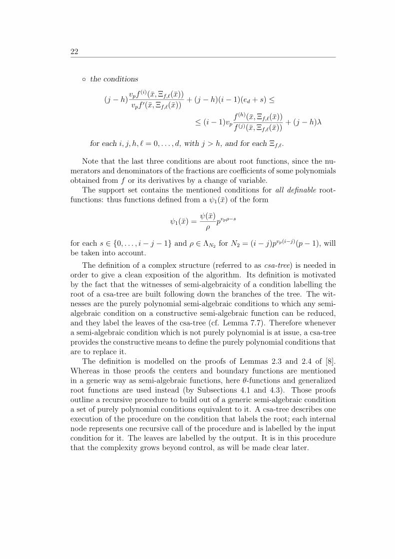
the conditions

(j − h)vpf

(i)(x,Ξf,`(x))

vpf ′(x,Ξf,`(x))+ (j − h)(i− 1)(ed + s) ≤

≤ (i− 1)vpf (h)(x,Ξf,`(x))

f (j)(x,Ξf,`(x))+ (j − h)λ

for each i, j, h, ` = 0, . . . , d, with j > h, and for each Ξf,`.

Note that the last three conditions are about root functions, since the nu-merators and denominators of the fractions are coefficients of some polynomialsobtained from f or its derivatives by a change of variable.

The support set contains the mentioned conditions for all definable root-functions: thus functions defined from a ψ1(x) of the form

ψ1(x) =ψ(x)

ρpvpρ−s

for each s ∈ 0, . . . , i− j − 1 and ρ ∈ ΛN2 for N2 = (i− j)pvp(i−j)(p− 1), willbe taken into account.

The definition of a complex structure (referred to as csa-tree) is needed inorder to give a clean exposition of the algorithm. Its definition is motivatedby the fact that the witnesses of semi-algebraicity of a condition labelling theroot of a csa-tree are built following down the branches of the tree. The wit-nesses are the purely polynomial semi-algebraic conditions to which any semi-algebraic condition on a constructive semi-algebraic function can be reduced,and they label the leaves of the csa-tree (cf. Lemma 7.7). Therefore whenevera semi-algebraic condition which is not purely polynomial is at issue, a csa-treeprovides the constructive means to define the purely polynomial conditions thatare to replace it.

The definition is modelled on the proofs of Lemmas 2.3 and 2.4 of [8].Whereas in those proofs the centers and boundary functions are mentionedin a generic way as semi-algebraic functions, here θ-functions and generalizedroot functions are used instead (by Subsections 4.1 and 4.3). Those proofsoutline a recursive procedure to build out of a generic semi-algebraic conditiona set of purely polynomial conditions equivalent to it. A csa-tree describes oneexecution of the procedure on the condition that labels the root; each internalnode represents one recursive call of the procedure and is labelled by the inputcondition for it. The leaves are labelled by the output. It is in this procedurethat the complexity grows beyond control, as will be made clear later.

23

A few comments on the approach that the procedure takes should improvethe understanding of the definition of csa-trees. The most intricated part isthe proof of semi-algebraicity of root and θ-functions. In both cases the idea isto replace the function at issue with a place-holder variable in the polynomialcondition in which it appears and to carry out the c.a.d. for the resultingpolynomial condition to obtain cell definitions. At this point, after havingsubstituted back the function for the place-holder variable, different cases mustbe considered as distinguished by the valuation and residue (modulo somepower of p) of the functions involved. In each case the conditions reduce toproblems which are analogous to the initial one but involve polynomials of asmaller degree (after Euclidean division).

It might be noticed that the procedure can follow one of a few strategies.Since it is irrelevant to our purposes which strategy is chosen, one is tacitlypicked and no further comment is made about the issue.

In the following, the functions Ξ are the generalized root functions defined inSection 4.3. The function f` is such that f`(x, ξf,`(x)θf,`(x)) = 0; it is obtainedfrom f via the change of variable y → Ξf,`−1 (this implies that f1 = f). Thefunctions θ and ψ, and the constant k are as in the definition of θ-functions (Def.4.5, Item 3). The variable z is meant to stand for an m-tuple of semi-algebraicfunctions.

Definition 5.3. (csa-tree) A csa-tree is a labelled tree recursively definedas follows:

1. Each node labelled by

h(x, z, γ(x)) = ρ · (nonzero n-th power)

for some polynomial h of degree dh, and semi-algebraic function γ whichis the root of a polynomial f of degree df < dh, has a child labelled by

r(x, z, γ(x)) = ρ · (nonzero n-th power)

where r(x, z, t) is the remainder of Euclidean division of h by f .

2. Each node labelled by

h

(x, z,

f1(x)

f2(x)

)= ρ · (nonzero n-th power)

24

for some f1, f2 ∈ C and polynomial h of degree dh, has a child labelled by

f2(x)νh

(x, z,

f1(x)

f2(x)

)= ρ · (nonzero n-th power)

where ν = minm ≥ dh s.t. n|m.

3. Each node labelled by

h(x, z,Ξf,`(x)) = ρ · (nonzero n-th power) (5.1)

for some polynomial h, of degree dh, smaller than the degree of the poly-nomial f` null at ξf,`(x)θf,`(x), has children labelled by the conditions inthe support set of condition (5.1), plus children labelled by

vp(Ξf,`(x)− Ξh,s(x, z)) ≤ vpθh,t(x, z) + i

and children labelled by

Ξf,`(x)− Ξh,s(x, z) = ρ · (nonzero µ-th power),

with µ = lcm(n,mλ+1,m2edh+λ), for each t ≤ s ≤ dh, i = −λ, . . . , 0 and

i = edh+ 1, . . . , edh

+ λ, and for each Ξh,s and θh,t (recall the notationalambiguity).

4. Each node labelled by

vp(Ξf,`(x)− Ξh,s(x, z)) ≤ vpΠh,t(x, z) + i

has children labelled by each one of the following conditions

vpΞf,`−1(x)−Ξh,s(x,z)

θf,`(x)≤ −λ

vpΞf,`−1(x)−Ξh,s(x,z)

θf,`(x)< 0

vpΞf,`−1(x)−Ξh,s(x,z)

θf,`(x)> 0

vp(Ξf,`−1(x)− Ξh,s(x, z)) ≤ vpθh,t(x, z) + i

Ξf,`−1(x)−Ξh,s(x,z)

θf,`(x)= ρ · (nonzero N -th power) with N = me`+2λ

f (j)(x,Ξf,`(x)) = ρ · (nonzero M -th power) for j = d− `, . . . , dwhere M = k ·m2e`+λ, and k is as in Def. 4.5, Item 3

vp

(−f`(x,Ξf,`−1(x)−Ξh,s(x,z))f ′

`(x,Ξf,`−1(x)−Ξh,s(x,z))

)≤ vpθh,t(x, z) + i.

25

5. Each node labelled by

Ξf,`(x)− Ξh,`h(x, z) = ρ · (nonzero n-th power)

has children labelled by each one of the following conditions

vpΞf,`−1(x)−Ξh,s(x,z)

θf,`(x)≤ −λ

vpΞf,`−1(x)−Ξh,s(x,z)

θf,`(x)< 0

vpΞf,`−1(x)−Ξh,s(x,z)

θf,`(x)> 0

Ξf,`−1(x)− Ξh,s(x, z) = ρ · (nonzero N -th power)with N = lcm(n,me`+3λ)

f (j)(x,Ξf,`(x)) = ρ · (nonzero M -th power) for j = d− `, . . . , dwhere M = k ·m2e`+3λ, and k is as in Def. 4.5, Item 3

−f`(x,Ξf,`−1(x)−Ξh,s(x,z))f ′

`(x,Ξf,`−1(x)−Ξh,s(x,z))= ρ · (nonzero n-th power).

6. Each node labelled by

h(x, z, θf,`(x)) = ρ · (nonzero n-th power) (5.2)

for some polynomial h of degree dh smaller than k (cf. Def. 4.5, Item3), has children labelled by the conditions in the support set of condition(5.2), children labelled by

vp(θf,`(x)− Ξh,s(x, z)) ≤ vpθh,t(x, z) + i

and children labelled by

θf,`(x)− Ξh,s(x, z) = ρ · (nonzero µ-th power)

with µ = lcm(n,mλ+1,m2es+λ), for each s, t ≤ dh, i = λ, . . . , 0 and i =ed + 1, . . . , ed + λ, and for each Ξh,s and θh,t.

7. Each node labelled by

vp(θf,`(x)− Ξh,s(x, z)) ≤ vpθh,t(x, z) + i

26

has children labelled by each one of the following conditions

vpψf,`(x) ≥ k(j + vpΞh,s(x, z)) for all j = −λ+ 1, . . . , 0, . . . , λvpψf,`(x) ≤ k(j + vpΞh,s(x, z)) for all j = −λ, . . . , 0, . . . , λ− 1vpψf,`(x) ≤ k(vpθh,t(x, z) + i)vpΞh,s(x, z) ≤ vpθh,t(x, z) + iψf,`(x) = ρ · (nonzero N -th power) with N = k ·mvpk+λ

Ξh,s(x, z) = ρ · (nonzero M -th power) with M = mvpk+λ

vpψ1(x)−Ξk

h,s(x,z)

kΞk−1h,s

(x,z)≤ vpθh,t(x, z) + i.

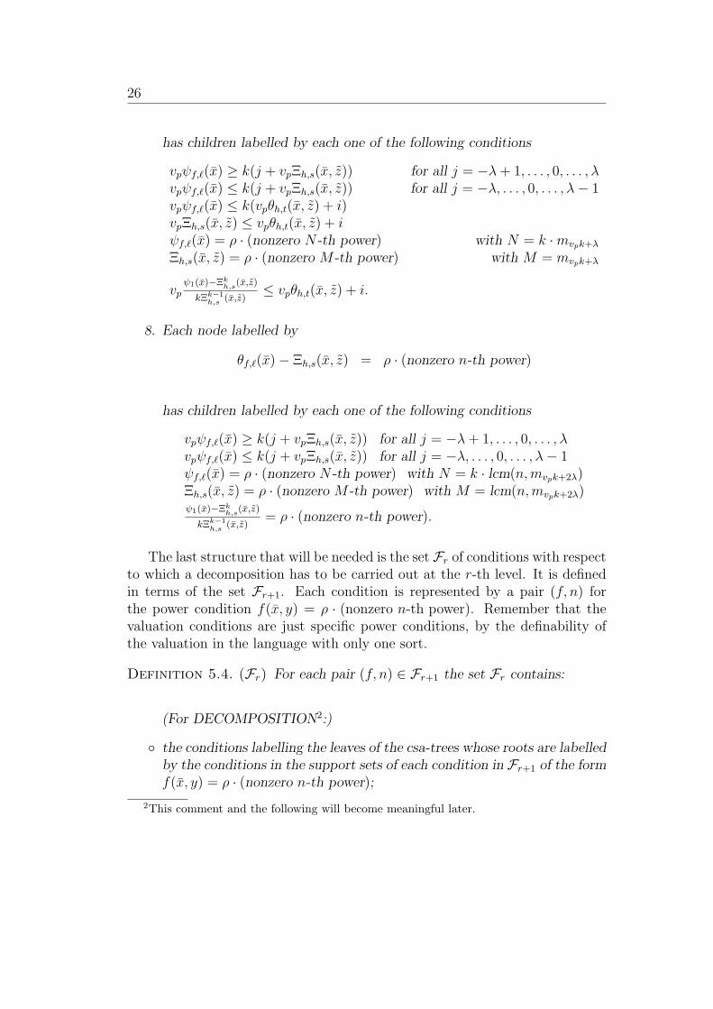
8. Each node labelled by

θf,`(x)− Ξh,s(x, z) = ρ · (nonzero n-th power)

has children labelled by each one of the following conditions

vpψf,`(x) ≥ k(j + vpΞh,s(x, z)) for all j = −λ+ 1, . . . , 0, . . . , λvpψf,`(x) ≤ k(j + vpΞh,s(x, z)) for all j = −λ, . . . , 0, . . . , λ− 1ψf,`(x) = ρ · (nonzero N -th power) with N = k · lcm(n,mvpk+2λ)Ξh,s(x, z) = ρ · (nonzero M -th power) with M = lcm(n,mvpk+2λ)ψ1(x)−Ξk

h,s(x,z)

kΞk−1h,s

(x,z)= ρ · (nonzero n-th power).

The last structure that will be needed is the set Fr of conditions with respectto which a decomposition has to be carried out at the r-th level. It is definedin terms of the set Fr+1. Each condition is represented by a pair (f, n) forthe power condition f(x, y) = ρ · (nonzero n-th power). Remember that thevaluation conditions are just specific power conditions, by the definability ofthe valuation in the language with only one sort.

Definition 5.4. (Fr) For each pair (f, n) ∈ Fr+1 the set Fr contains:

(For DECOMPOSITION2:)

the conditions labelling the leaves of the csa-trees whose roots are labelledby the conditions in the support sets of each condition in Fr+1 of the formf(x, y) = ρ · (nonzero n-th power);

2This comment and the following will become meaningful later.

27

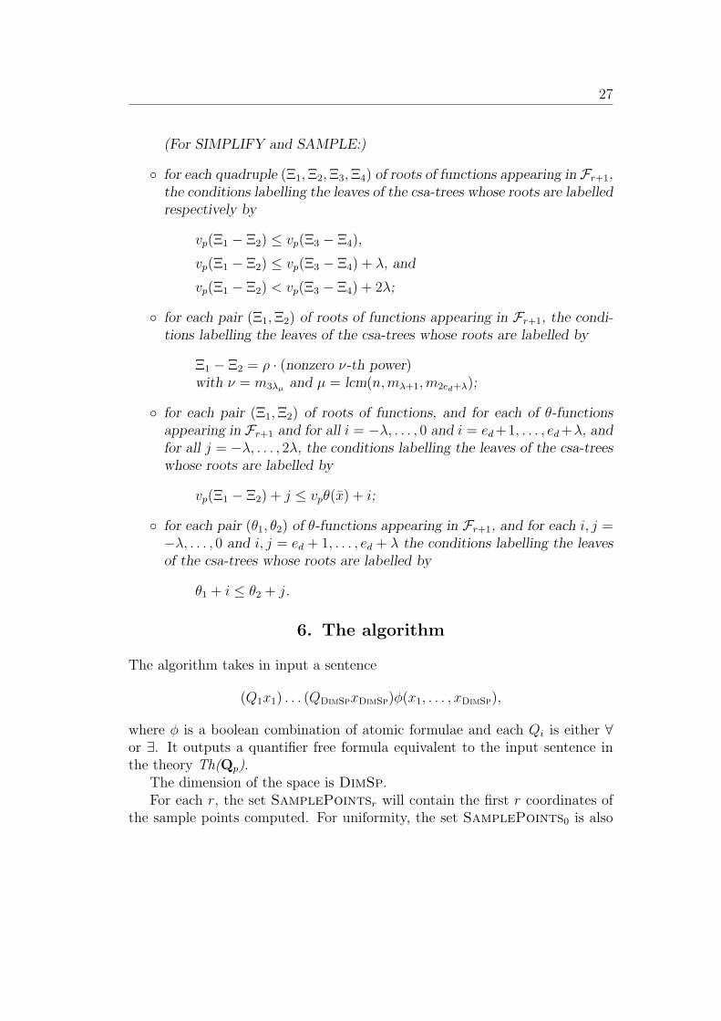
(For SIMPLIFY and SAMPLE:)

for each quadruple (Ξ1,Ξ2,Ξ3,Ξ4) of roots of functions appearing in Fr+1,the conditions labelling the leaves of the csa-trees whose roots are labelledrespectively by

vp(Ξ1 − Ξ2) ≤ vp(Ξ3 − Ξ4),

vp(Ξ1 − Ξ2) ≤ vp(Ξ3 − Ξ4) + λ, and

vp(Ξ1 − Ξ2) < vp(Ξ3 − Ξ4) + 2λ;

for each pair (Ξ1,Ξ2) of roots of functions appearing in Fr+1, the condi-tions labelling the leaves of the csa-trees whose roots are labelled by

Ξ1 − Ξ2 = ρ · (nonzero ν-th power)with ν = m3λµ and µ = lcm(n,mλ+1,m2ed+λ);

for each pair (Ξ1,Ξ2) of roots of functions, and for each of θ-functionsappearing in Fr+1 and for all i = −λ, . . . , 0 and i = ed+1, . . . , ed+λ, andfor all j = −λ, . . . , 2λ, the conditions labelling the leaves of the csa-treeswhose roots are labelled by

vp(Ξ1 − Ξ2) + j ≤ vpθ(x) + i;

for each pair (θ1, θ2) of θ-functions appearing in Fr+1, and for each i, j =−λ, . . . , 0 and i, j = ed + 1, . . . , ed + λ the conditions labelling the leavesof the csa-trees whose roots are labelled by

θ1 + i ≤ θ2 + j.

6. The algorithm

The algorithm takes in input a sentence

(Q1x1) . . . (QDimSpxDimSp)φ(x1, . . . , xDimSp),

where φ is a boolean combination of atomic formulae and each Qi is either ∀or ∃. It outputs a quantifier free formula equivalent to the input sentence inthe theory Th(Qp).

The dimension of the space is DimSp.For each r, the set SamplePointsr will contain the first r coordinates of

the sample points computed. For uniformity, the set SamplePoints0 is also

28

defined as the set containing the single element 0, which (again for uniformity)will be considered to be a tuple of length 0.

Since so far when discussing a generic stage of the algorithm the focus wason the (r+ 1)-st variable, the outer loop in the algorithm has r ranging from 0to DimSp−1, and in the r-th loop the (r+1)-st variable is under consideration.

The inner recursion is implemented using the sets CallJr+1. These sets helpmanage the recursive calls to DECOMPOSITION. Each 5-tuple

(f, n,Var,Cell, eJ−1)

in CallJr+1 specifies the condition (f, n) with respect to which the space must bedecomposed, keeps track of the changes of variable that have been performedso far on the (r + 1)-st variable (through Var), of the cell definition attainedso far and that has to be further decomposed while working on the (d− J)-stderivative of f (through Cell), and of the value of the parameter eJ−1 (recallits recursive definition).

For each J = 1, . . . ,maxd|d = degree off ∈ Fr+1, the variables CadJare used to memorize the definition of the r + 1-st dimension of the cells. Thevariable Cad will eventually hold the global definition of the cells in whichQDimSpp is partitioned.

Algorithm: QuantifElimInput: a sentence Φ = ((Q1x1) . . . (QDimSpxDimSp)φ(x1, . . . , xDimSp)) where φ isa boolean combination of atomic formulae and each Qi is either ∀ or ∃.Output: a quantifier free formula QFFormula equivalent to the input sentencein the theory Th(Qp).Description:

Let n = lcmm| the predicate Pm appears in some atomic formula in φ.

F =INIT(φ, n).

Let λ = 2vpn+ 1.

Let SamplePoints0 = 0.

For r = 0 to DimSp− 1 do:

For each r-tuple x0 ∈ SamplePointsr do:

∗ Let Call1r+1 = (f, n, xr+1, 1, 0)|(f, n) ∈ Fr+1

29

∗ Let M = maxd|d = degree off ∈ Fr+1,

∗ For each J = 2, . . . ,M ,let CallJr+1 = ∅.

∗ Let Cnt = 0.

∗ For J = 1 to M do:For each 5-tuple T ∈ CallJr+1

call DECOMPOSITION(J, T ).

∗ For J = 0 to Cntlet CadJ = SIMPLIFY(CadJ).

∗ Let Cad =⋃CntJ=1 CadJ .

∗ Let Cad =SIMPLIFY(Cad).

∗ Let SamplePointsr+1 =SAMPLE(Cad, x0)

Let QFFormula = EVALUATE(Φ,SamplePointsDimSp)

Output QFFormula

Procedure: INIT

Input: a formula φ and a positive integer n which is the least common multipleof the integers m such that a predicate Pm appears in φ.

Output: sets Fr (r = 1, . . . ,DimSp) such that FDimSp contains for each atomicformula in φ a power condition that implies it, and for all other r, Fr is obtainedfrom FDimSp according to Definition 5.4.

Description:

Let FDimSp = (fi, n)|fi is a polynomial appearingin some atomic formula in φ.

For r = DimSp− 1 downto 1 define Fr, according to Definition 5.4.

30

Procedure: DECOMPOSITIONInput: the pair (J, T ) where J defines the step of the inner recursion and T isa 5-tuple from CallJr+1 (see the initial part of this section).Output: if J is smaller than f ’s degree, the output is CallJ+1

r+1 , otherwise theoutput is CadCnt (the definition of the (r + 1)-st dimension of the cell).Description:

1. Let y = Var. Perform a change of variable: write f(x, xr+1) as a functionof y = Var.Let d be the degree of f .

2. For each pair (i, j) (i, j ∈ 0, . . . , d) and for each s ∈ 0, . . . , i− j − 1and ρ ∈ ΛN2 for N2 = (i − j)pvp(i−j)(p − 1), of indexes of monomials off (d−J), define θij(x).

3. Let eJ = vpi0 + eJ−1.

4. Define the (r + 1)-st dimension of the space decomposition as follows:

(a) For each i0, and ρ ∈ Λn define the following cells:

Cell(i0)λ = Cell ∧

∧j<i0

vpθi0j(x)− vpy ≥⌈

λ

i0 − j

⌉∧

∧∧j>i0

vpθi0j(x)− vpy ≤⌈

λ

i0 − j

⌉∧

∧ y = ρ · (nonzero n-th power)

(b) For each s = 1, . . . , λ − 1, pair (i0, j) and σ ∈ ΛN with N = mλ,define the following cells:

Cell(i0j)s = Cell ∧ vpy = vpθi0j(x)−

⌈s

i0 − j

⌉∧

∧∧h<i0

vpθi0j(x) ≤ vpθi0h(x) ∧

∧∧h>i0

vpθi0h(x) ≤ vpθi0j(x) ∧

y = σ · (nonzero N -th power)

(c) For each pair (i, j) and σ ∈ ΛN with N = m2eJ+λ, such that

f(x, θ(x)σ) < 2eJ + vp(ai0(x)θij(x)),

31

define the following cells:

Cell(ij) = Cell ∧ vpy = vpθij(x)∧∧ y = σ · (nonzero N -th power)

(d) For each pair (i, j), ρ ∈ Λn and σ ∈ ΛN with N = m2eJ+1, such that

f(x, θ(x)σ) ≥ 2eJ + vp(ai0(x)θij(x)),

define the following cells:

Cell(ij)0λ = Cell ∧ vpy = vpθij(x)∧

∧ vp(y − ξij(x)θij(x)) ≥ vpθij(x) + eJ + λ ∧∧ y − ξij(x)θij(x) = ρ · (nonzero n-th power) ∧∧ y = σ · (nonzero N -th power)

where ξij(x) is defined by

f(x, ξij(x)θij(x)) = 0 ∧ ξij(x) ≡ σ mod p2eJ+1

(by Hensel’s Lemma it is well defined).

(e) For each pair (i, j), for each ρ ∈ ΛM , with M = lcm(mλ+1, n) foreach σ ∈ ΛN with N = m2eJ+1, such that

f(x, θ(x)σ) ≥ 2eJ + vp(ai0(x)θij(x)),

and for s = 0, . . . , λ− 2 define the following cells:

Cell(ij)0s = Cell ∧ vpy = vpθij(x) ∧

∧ y = σ · (nonzero N -th power) ∧∧ vp(y − ξij(x)θij(x)) ≥ vpθij(x) + eJ + s+ 1 ∧∧ y − ξij(x)θij(x) = ρ · (nonzero M -th power)

where ξij(x) is defined as in the previous Item.

5. Expand y as Var in the cell-defining conditions.

6. If J < d do:

(a) For each cell defined in 4a. set

CallJ+1r+1 = CallJ+1

r+1

⋃(f, n,Var,Cell(i0)λ , 0).

32

(b) For each cell defined in 4b. setCallJ+1

r+1 = CallJ+1r+1

⋃(f, n,Var,Cell(i0j)s , 0).

(c) For each cell defined in 4c. setCallJ+1

r+1 = CallJ+1r+1

⋃(f, n,Var,Cell(ij), 2eJ).(d) For each cell defined in 4d. set

Var = Var− ξij(x)θij(x)

CallJ+1r+1 = CallJ+1

r+1

⋃(f, n,Var,Cell(ij)0λ , 0).

(e) For each cell defined in 4e. setVar = Var− ξij(x)θij(x)

CallJ+1r+1 = CallJ+1

r+1

⋃(f, n,Var,Cell(ij)0s , 0).

7. else, if J = d, do:

Cnt = Cnt + 1.

CadCnt =⋃

Cell(i0)λ ∪ ⋃

Cell(i0j)s ∪

∪⋃Cell(ij) ∪ ⋃Cell(ij)0λ ∪ ⋃

Cell(ij)0s .

Procedure: SIMPLIFYInput: the (r+1)-st dimension SetOfCells of a decomposition in cells of thespace.Output: an equivalent decomposition SetOfCells in which each cell is definedby a single power condition and a single valuation condition.Description:

Let I = 0.For each center ξ(x) of some cell in SetOfCells

– let Center[I] = ξ(x);

– I = I + 1.

Let Boundaries = α(x)| such that vpα(x) is in a condition for somecell

in SetOfCells ∪ Center[i]−Center[j]|i < j.

Let N = lcmm| y −Center[I] = ρ · (nonzero m-th power)appears in some cell of SetOfCells.

Let SetOfCells = ∅.

33

For each I, for each ρ ∈ ΛN and for each pair (i, j) such that αi(x) andαj(x) are in Boundaries, let

SetOfCells = SetOfCells ∪vpαi(x) + λ ≤ vp(xr+1 −Center[I]) < λ+ αj(x)∧

xr+1 −Center[I] = ρ · (nonzero N -th power)∪vpαi(x) + λ ≤ vp(xr+1 −Center[I]) < 2λ+ αj(x)∧

xr+1 −Center[I] = ρ · (nonzero N -th power)∪vpαi(x) + λ ≤ vp(xr+1 −Center[I])∧

xr+1 −Center[I] = ρ · (nonzero N -th power)∪vp(xr+1 −Center[I]) < λ+ αj(x)∧

xr+1 −Center[I] = ρ · (nonzero N -th power)∪vp(xr+1 −Center[I]) < 2λ+ αj(x)∧

xr+1 −Center[I] = ρ · (nonzero N -th power)

Return SetOfCells.

Procedure: SAMPLEInput: the (r + 1)-st dimension SetOfCells of a decomposition in cells ofthe space in which each cell is defined by a single power condition and a singlevaluation condition.Output: a set NewPoints of sample points in Qr+1

p such that there is at leastone point in NewPoints

⋂C for each cell C in the c.a.d. of Qr+1

p .Description:

Let NewPoints = ∅.

For each cell in SetOfCells, of the form

vpα1(x) ≤ vp(xr+1 −Center[I]) < vpα2(x) ∧xr+1 − ξ(x) = ρ · (nonzero N -th power),

and for all c ∈ ΛN , let

NewPoints = NewPoints ∪ (x10, . . . , xr0, α1(x0)c+ ξ(x0)),

where x0 = (x10, . . . , xr0).

For each cell in SetOfCells, of the form

vp(xr+1 −Center[I]) < vpα1(x) ∧xr+1 − ξ(x) = ρ · (nonzero N -th power),

34

and for all c ∈ ΛN , let

NewPoints = NewPoints ∪ (x10, . . . , xr0, α1(x0)cp−N + ξ(x0)),

where x0 = (x10, . . . , xr0).

Return NewPoints.

The actual elimination of quantifiers is exactly like Collins’ for the reals.

Procedure: EVALUATEInput: the pair (Φ,SamplePointsDimSp) where Φ is a prenex sentence

(Q1x1) . . . (QDimSpxDimSp)φ(x1, . . . , xDimSp),

with each Qi being either ∃ or ∀, and SamplePointsDimSp is the set of samplepoints of the c.a.d. of Qr+1

p relative to Φ.Output: a quantifier free formula QFFormula equivalent in the theory to thesentence in input.Description:

SetQFFormula = (B1)i1 . . . (BDimSp)iDimSp

φ(β1,i, . . . , βiDimSp)

where for each r = 1, . . . ,DimSp

– if Qr = ∃, then (Br) =∨

;

– if Qr = ∀, then (Br) =∧

;

and ir ranges over the r-th coordinates of the sample points.

Return QFFormula.

7. Correctness

The correctness of the algorithm depends on the correctness of the single pro-cedures that it consists of and therefore the latter will be analyzed one byone.

A couple of technical results are in order first.It will be often useful to split the space in cells in each one of which some

function has a constant residue modulo pα for some α. The lemma below andits corollary provide a useful tool to this end.

35

Lemma 7.1. For any function f(x) : Qrp → Qp, acf(x) has constant residue

modulo pα if f(x) is in a fixed coset of themα-th powers, withmα = pα−1 (p−1).

Proof. Since pα−1(p − 1) is the order of the group of units of Zp/pα,

Pmα(acf(x)) implies acf(x) ≡ 1 mod pα. Now consider any representative h of

the residue class modulo pα: Pmα(acf(x)h

) implies acf(x) ≡ h mod pα.If f(x) = h · u(x)mα for some constant h, then acf(x) = ach · ac(u(x)mα).Because of the choice of mα, u(x)

mα ≡ 1 mod pα and the claim follows. 2

Corollary 7.2. (Constant Residue Mod pα) For any f(x) : Qrp → Zp,

if f(x) is in a fixed coset of the mα-th powers, and vpf(x) is either alwayssmaller than α, or always greater than or equal to it , then f(x) has constantresidue modulo pα.

Notice that if 0 ≤ vpf(x) ≤ k for some positive rational integer k, if f(x)has a constant residue modpλ+k, then it is in a fixed coset of the n-th powers.

Let us now consider a root-function ξ(x) of some g(x, t) as in Def. 4.5.

Lemma 7.3. (Congruences and root-functions) Let the functions ξ(x)and g(x, t) be as in Item 2 of Def. 4.5 above. The residue modulo pα of ξ(x)depends on the residues modulo e+ α of the coefficients of g(x, t) viewed as apolynomial in t.

Proof. Let x, x′ be such that the coefficients of g(x, t) and those of g(x′, t)are equivalent modulo pe+α. The Taylor expansion of g(x, t) in a neighborhoodof ξ(x) computed at ξ(x′) is

g(x, ξ(x′)) = g′(x, ξ(x))(ξ(x′)− ξ(x)) + f1(x)(ξ(x′)− ξ(x))2 + . . .

The first term of the expansion has valuation smaller than the rest, since:vp(ξ(x

′)−ξ(x)) ≥ e+1 because both ξ(x) and ξ(x′) are by hypothesis congruentto k modulo pe+1; vpg

′(x, ξ(x)) ≤ e again by hypothesis; and f1(x) and all thesuccessive coefficients of the expansion take values in Zp. Therefore

vpg(x, ξ(x′)) = vpg

′(x, ξ(x)) + vp(ξ(x′)− ξ(x)) ≤ e+ vp(ξ(x

′)− ξ(x)).

Note that, because of the hypothesis on the coefficients of g(x, t) and g(x′, t), thevaluation of g(x, ξ(x′)) is not smaller than e+α, and therefore vp(ξ(x

′)−ξ(x)) ≥α as required. 2

36

Therefore by splitting the r-dimensional space in cells in each of which thecoefficients of g(x, t) as a polynomial in t have a constant residue modulo pe+α,it is obtained that in each cell ξ(x) has a fixed residue modulo pα.

The conditions on ξ’s residue modulo some power of p are conditions onthe coefficients of g, i.e. on the coefficients of f and on some θ-function (up tomultiplicative constants).

Let us now analyze each one of the procedures that have been presented.

Lemma 7.4. (DECOMPOSITION) For any r ∈ 1, . . . ,DimSpace − 1,consider at the r-th stage of the outer recursion a call to DECOMPOSITIONwith arguments J and T , where T is the 5-tuple (f, n,Var,Cell, eJ−1), Jdefines the step of the inner recursion and (f, n) the power condition withrespect to which the space has to be decomposed, Var specifies the change ofvariable that has been performed at the previous stage, Cell describes the cellof the decomposition that has to be further split, eJ−1 is the constant Constfrom Item 3 in Subsection 4.1.

The procedure defines the r + 1-st dimension of cells in each one of which

f (d−J)(x, xr+1) = ρ · (nonzero n-th power)

provided that the r-dimensional space has been split in cells in each one ofwhich the conditions in the relevant support set are satisfied.

Proof. The present lemma simply summarizes the results already discussedin Section 4.1. 2

Lemma 7.5. (SIMPLIFY) Consider a call to the procedure SIMPLIFY withargument the (r+ 1)-st dimension SetOfCells of a decomposition in cells ofthe space. It yields in output an equivalent decomposition in which each cellis defined only by two conditions of the form

y − χ(x) = ρ · (nonzero n-th power), (7.1)

vpa1(x)21vp(y − χ(x))22vpa2(x) (7.2)

for some constructive semialgebraic functions χ(x), a1(x) and a2(x), and where21 stands for ≤ or no condition at all and 22 for < or no condition at all,provided that the r-dimensional space has been split in cells in each one of

37

which:

vp(χ1(x)− χ2(x)) < vp(χ3(x)− χ4(x)) + i with i = 0, λ, 2λχ1(x)− χ2(x) = ρ · (nonzero ν-th power) with ν = m3λµ

and µ = lcm(n,mλ+1,m2ed+λ)vp(χ1(x)− χ2(x)) + j ≤ vpθ(x) + i with j = −λ, . . . , 2λ

and for each i = −λ, . . . , 0 and i = ed + 1, . . . , ed + λ;θ1 + i ≤ θ2 + j

for each i, j = −λ, . . . , 0 and i, j = ed + 1, . . . , ed + λ,

for each quadruple of centers (χ1(x), χ2(x), χ3(x), χ4(x)) and for each triple(θ, θ1, θ2) of θ-functions appearing in the cells of SetOfCells.

Proof. The first step of the proof is to examine the problem from a theo-retical point of view, by quickly reminding the proof from [8], p.163-164.

Let C be a cell with two centers, χ1(x) and χ2(x).First the cell must be split into two subcells:

(x, y) ∈ C|χ1(x) = χ2(x)and (x, y) ∈ C|χ1(x) 6= χ2(x).

The first of the two subcells needs no further attention. The other is to be splitaccording to the following cases:

1. In the subcells in which

vpy − χ1(x)

χ2(x)− χ1(x)≥ λ,

all conditions on y − χ2(x) can be replaced by the analogous conditionson χ2(x)− χ1(x).

2. In the subcells in which

vpy − χ1(x)

χ2(x)− χ1(x)< −λ,

y − χ2(x) can be replaced in all conditions by y − χ1(x).

3. In the subcells in which

pλ(y − χ2(x))

χ2(x)− χ1(x)≡ 0 mod p2λ,

χ2(x)− χ1(x) can replace y − χ1(x) in all conditions.

38

4. In the subcells in which

pλ(y − χ2(x))

χ2(x)− χ1(x)≡ a mod p3λ,

where a ∈ Zp, vpa < 2λ, a 6≡ −pλ mod p2λ (the case a ≡ −pλ mod p2λ

reduces to Case 1), all conditions involving y − χ1(x) can be replaced byconditions on p−λ(χ2(x)− χ1(x))(a+ pλ).

The four items above cover all the possible cases, as can be checked consideringthat

pλ(y − χ1(x))

χ2(x)− χ1(x)=pλ(y − χ2(x))

χ2(x)− χ1(x)+ pλ.

Let Centers be the set of all centers appearing in a cell. Fix some arbitraryorder in the set appearing in a cell. Repeating the above steps subsequentlyfor the pair of centers (χi, χi+1), for each i up to the cardinality of the set(minus one), only one center eventually remains. (The reference to the pair isnot totally accurate, but is meant to be intuitive.)

The procedure SIMPLIFY takes a short cut to achieve the same goal.Following the process closely, it can be seen that the cells obtained are

defined by conditions of the form

vp(y − χ(x)) ≥ vp(χj2(x)− χj1(x)) + λvp(y − χ(x)) < vp(χj4(x)− χj3(x)) + λvp(y − χ(x)) < vp(χj6(x)− χj5(x)) + 2λy − χ(x) = ρ · (nonzero m3λ-th power)

with χji ∈ Centers, and a subset of all the conditions defining the cell, allwritten by substituting the old center with χ(x).

If the r-dimensional space has been decomposed so that in each cell the val-uations of all the boundary functions (including the newly introduced (χj(x)−χi(x)) + λ and (χj(x)− χi(x)) + 2λ for all pairs of centers) are always distinctand in a constant relation to each other (one is greater in the whole cell), allof the above conditions involving the valuation can be substituted by a singleone of the form (7.2).

All of the other conditions can be substituted by a single one of the form(7.1) where n is the least common multiple of all the powers appearing, sinceall power conditions are on y − χ(x) for a single center χ(x). 2

39

Lemma 7.6. (SAMPLE) Let

y − χ(x) = ρ · (nonzero n-th power),

vpa1(x) ≤ vp(y − χ(x))2vpa2(x),

(where 2 is either < or no condition at all) and

y − χ(x) = ρ · (nonzero n-th power),

vp(y − χ(x)) ≤ vpa1(x),

be the definitions of the (r + 1)-st dimension of cells in the set SetOfCells.The procedure SAMPLE outputs a set NewPoints of sample points in Qr+1

p

such that there is at least one point in NewPoints⋂C for each cell C in the

decomposition of Qr+1p , provided that the r-dimensional space has been split

in cells such that for each one of them there exists a γ ∈ Λn for which

Pn(a1(x)ρ

−1γ)

holds in the cell.

Proof. Let x0 be the first r coordinates of the sample points.Consider the first case, i.e. vp(y − χ(x)) is bounded from below. In this casethe values for the (r + 1)-st coordinate of the sample points chosen are y0 =a1(x0)c + χ(x0)) where c ∈ ΛN . Let γ0 be such that Pn (a1(x)ρ

−1γ0) holds inthe cell. It will be proven later (see Lemma 8.1) that the coset representativescan be chosen in N and of valuation smaller than n. Then

vp(y0 − χ(x0)) = vp(a1(x0)γ0) ≥ vpa1(x0) and

y0 − χ(x0) = a1(x0)γ0 = ρ · (nonzero n-th power).

If the 2 stands for a <, the point belongs to the cell only if

vpa1(x0) + vpγ0 < vp(a2x0)

but this is a necessary and sufficient condition for the cell to be non empty (cf.[8], p.165).

If the cell is empty and in any case for all coset representatives c 6= γ0

the points picked are not in the cell. But insofar as each non empty cell is

40

represented by a sample point and the complexity doesn’t increase exceedingly,the policy is acceptable.

If on the other hand vp(y−χ(x)) is not bounded below in the cell definition,it can still be bounded artificially, say by vpa1(x) − n (the resulting cell is forsure non empty in this case). Then the same argument given above proves thecorrectness of the sampling procedure in this case too. 2

In each one of the above lemmas appears a proviso involving conditions ofone less variable. The algorithm works properly if all those conditions appearin the set Fr. Indeed this is not possible in general because many of thoseconditions are not purely polynomial. But for each semi-algebraic conditionin the provisos, the conditions labelling the leaves of the csa-tree whose rootis labelled by that condition can (and indeed do) appear in Fr. The followinglemma explains why it should be so.

Lemma 7.7. (csa-tree) The leaves of a csa-tree whose root is labelled by asemi-algebraic condition

h(x, z, γ(x)) = ρ · (nonzero n-th power)

for some constructive semi-algebraic function γ(x) are labelled by purely poly-nomial semi-algebraic conditions. If the space is split in cells in each one ofwhich all the conditions labelling the leaves are verified, then so is in each cellthe condition labelling the root.

This statement is essentially the proof of Lemma 4.6. Its proof is obtainedby checking that for each item in the definition of a csa-tree, splitting thespace with respect to all the conditions labelling the children, yields a spacedecomposition for the parent node. The finiteness of the tree follows from thefact that the degree in each (place-holder) variable of the polynomials appearingis decreasing down the tree (keep in mind Item 1 of the definition of csa-trees).

Thanks to the knowledge just acquired about the csa-trees, it can be directlychecked that the sets Fr are defined correctly. Notice that in the definition ofFr a hint is given as to which conditions are needed by each procedure.

The proof of correctness can be now completed:

Proposition 7.8. (Correctness) The algorithm QuantifElim computes aquantifier free formula equivalent in Th(Qp) to the formula it takes in input.

Proof. The lemmas above prove that each one of the procedures that thealgorithm relies on performs its duty at the (r + 1)-st stage, provided that

41

some sets of conditions on r variables are satisfied by the decomposition of ther-dimensional space. The procedure INIT defines the sets Fr of conditions tobe considered at each stage in such a way that the above is guaranteed—as hasjust been pointed out.

The procedure EVALUATE performs the actual elimination of quantifiersby making use of the sample points. Its correctness is based on the “cylin-drical” structure of the cells that allows a separate treatment of the differentcoordinates of each sample point.

The correctness of the whole algorithm follows. 2

8. The complexity

The complexity is analyzed by first estimating essentially the number of con-ditions and the maximum powers occurring in the tools defined in Section 5.Then the coefficients’ growth and the lengths of conditions and sample pointsare evaluated. All the bounds thus derived are eventually used in the complex-ity analysis of the single procedures.

Throughout, the maximum degree d of the polynomials involved appears asa parameter. Its growth is analyzed separately in order to isolate more clearlythe complexity explosion. Indeed, the degree of the polynomials involved growin a non-elementary fashion thus blowing up the whole bound.

8.1. Analysis of the support structures. Let d be the maximum of thedegrees of f in each variable.

As was mentioned earlier, it is possible to establish a bound on the numberof cosets of the n-th powers, for any n:

Lemma 8.1. (Number of cosets) For each choice of n and p there are atmost pλ cosets of the n-th powers in Qp, where λ = 2vpn+ 1. For each coset arepresentative c such that vpc < λ can be chosen.

Proof. The proof follows from Lemma 4.9, observing that any p-adic numberw can be written as a product m · u, where m is the residue of w modulo pλ

and, as a consequence, u ≡ 1 (mod pλ). There are pλ residues modulo pλ, andtheir canonical representatives have valuation smaller than λ. 2

The following lemma gives an upper bound to the number of generalizedroot and θ-functions. It counts all the θ-functions that can be defined, sinceit is necessary for the correctness of the algorithm that they be all consideredwhen building the sets Fr.

42

Lemma 8.2. (θ-functions and roots) For a polynomial f of degree d, atmost d8 θ-functions θf,d and d!8 (i.e. O(d8d)) generalized root-functions Ξ canbe defined.

Proof. A polynomial of degree d has at most d+1 coefficients which amountsto (d + 1)d pairs of distinct coefficients, and therefore functions ψij(x). Onefunction θf,d must be defined for each

ψ1(x) = ψij(x)pvpρ−s

ρ

where s ranges over 0, . . . , i−j−1 and ρ over ΛN2 forN2 = (i−j)pvp(i−j)(p−1).This means that for each ψij, at most (i − j)p4vp(i−j)+1 ≤ (i − j)6 functionsθf,d can be defined (cf. Lemma 8.1 for the cardinality of ΛN2). Thus for apolynomial of degree d at most (d + 1) · d · d6 functions θf,d can be defined.By the definition of generalized root functions and by the remark above onthe number of root-functions that must be considered, the generalized root-functions are d!8 (for each ` = 1, . . . , d one θf,` must be chosen). 2

A bound on the value of the constant es that at each stage of the innerrecursion bounds the valuation of the function g′f,s, must be established.

Lemma 8.3. (es) The constant es that bounds the valuation of the functiong′f,s, where gf,s is built from f (d−s) (cf. Section 4.1), is smaller than 2s−2s.

Proof. The discussion in Section 4.1 amounts to the following recursivedefinition of es:

es =

(vpi0)s if f (s+1) had a root or

vpbi(x)yi 6= vpbj(x)y

j( for all i, j)(ordi0)s + 2es−1 otherwise

where (vpi0)s denotes here the valuation of the integer i which is the index ofthe monomial of minimum valuation in the cell at issue and at the s-th step ofthe inner recursion.Therefore es ≤ k0 + 2es−1 for k0 ≤ maxi=1,...,svpi and e1 = 0, i.e. es < 2s−2s.

2

On the basis of the above results rests the complexity analysis of the supportstructures defined in Section 5.

Lemma 8.4. (Support set) The support set of a condition

f(x, y) = ρ · (nonzero n-th power)

43

has size O((d+ 1)4d!8) and the maximum power appearing in the conditions isO(p2d · n2).

Proof. Let us count the number of conditions in each item in the definitionof the support set. In the first item there are (d + 1)d!8 conditions (one foreach choice of i and generalized root); similarly, there is the same number ofconditions in the second item; in the third one there are (d + 1)4d!8, in thefourth 2(d+ 1)3d!8 and in the last one (d+ 1)3d!8. The sum is O((d+ 1)4d!8).The maximum power involved is N = lcmh=1,...,d(hmvph+1, hm2ed+λ, hn). Bythe bound just derived on ed, N ≤ lcmh=1,...,d(hmvph+1, hm2d−1d+λ, hn);mvph+1 is a factor of m2d−1d+λ and can be therefore disregarded in the leastcommon factor; pλ ≤ n2p; p − 1 < p; the least common factor is smaller thand! · p2d−1d+1n2 which is O(p2d · n2). 2

Lemma 8.5. (Leaves of a csa-tree) A csa-tree whose root is labelled bythe polynomial form h(x, ξ(x)), where h(x, t) is a polynomial of degree d in t,

has O((vpn)2d) leaves with maximum power condition of order O(n22d

p22d

).

Proof. The tree is finite. Indeed, each node is labelled by a polynomialform of lesser degree than its parent in each variable (even though the numberof variables might be increasing).

In order to give a bound on the number of leaves in the tree it is sufficientto give a bound on the depth of the tree and on the number of children thateach node can have.

Let us examine each item of the definition of a csa-tree in an omologousenumeration.

1. Only one child.

2. Only one child.

3. O(d!8) children labelled by the conditions in the support set; d!8 powerconditions and d!8d8(2λ+1) valuation conditions (the latter resulting fromd!8 possible generalized root-functions, d8 possible θ-functions, times allthe possible choices for i). The total here is O(d!8(2 + d8(2λ + 1))) =O(d!82λ).

4. d+ 7 children, d+ 1 being conditions on f ’s derivatives.

5. d+ 6 children, here too including conditions on f ’s derivatives.

44

6. Same as Item 3.

7. 4λ+ 7 children.

8. 4λ+ 7 children.

The maximum number of children that one node can have is O(d!8λ).

The children of each node are labelled by conditions on polynomial formswhich might be on more semi-algebraic functions. Up to 2d, can be added toa polynomial form of degree d (d root-functions and d θ-functions). But thedegree of the resulting polynomial forms in each one of the new functions isstrictly smaller than d. Because of this the process can be repeated at most dtimes. The total count of the new variables introduced is thus

2d · 2(d− 1) · 2(d− 2) · · · 2 = 2dd!.

Each one is dealt with in at most d successive levels. Therefore the depth ofthe tree is bounded by d2dd!.

In order to put together the bounds on the fan-out and the depth of thecsa-tree, the growth of n, and therefore of λ, down the tree must be analyzed.Again the proof follows the pattern of the definition of csa-trees.

1. n doesn’t change.

2. n doesn’t change.

3. In the support set n grows to O(p2d · n2); valuation conditions are equiv-alent to power residue conditions with power 2 or 3; in the power residuecondition, n grows to O(n2p2d

) (this bound is derived in a way similar tothe one for the support set). Globally, n grows to O(n2p2d

) here.

4. The growth is in one case to me`+2λ, in the other to k · m2e`+λ; that is

O(p2dn).

5. n grows to lcm(n,me`+3λ) and to k ·m2e`+2λ; i.e. O(p2dn2) .

6. Same as Item 3.

7. n grows to k ·mvpk+λ; this is O(d2n).

8. n grows to k · lcm(n,mvpk+2λ); the order of growth is here O(d2n).

45

The powers involved in the conditions labelling the children of a node whosecondition is on the n-th powers is O(n2p2d

). This implies that through a depth

of d2dd!, n increases to O(n22d

p2d22d

) which is also O(n22d

p22d

).

The number of leaves of a tree of fan-out w and depth h is wh−1. The leavesof the csa-tree are O((22d

vpn+ 22d)2d

) which is O((vpn)2d). 2

Lemma 8.6. (Power conditions in sets Fr) If n is the maximum power

appearing in Fr+1, then the maximum power appearing in Fr is O(n22d

p22d

).

Proof. The proof will follow the structure of the definition of sets Fr:

The maximum power in the conditions in the support set is O(p2d · n2).

The valuation conditions are conditions on the 2nd or 3rd power residue,depending on p.

Here the power is m3λµ and µ = lcm(n,mλ+1,m2es+λ) is the highest power

involved in conditions labelling roots of csa-tree and it is O(n2p2d).

The conditions are on 2nd or 3rd power residues.

Again the conditions are on 2nd or 3rd power residues.

But in the sets Fr there are the leaves of the csa-tree labelled by them. There-

fore by the preceding lemma, the power grows to O(n22d

p22d

). 2

At this point the maximum n involved in the power condition dependingfrom the input can be computed.

Corollary 8.7. (nmax) Let n be the power in the conditions in FDimSp. Thenthe algorithm will have to deal at most with nmax-th power residues, where

nmax = O((pn)22dDimSp

).

Proof. Considering that the growth of n proven in the lemma above isrepeated DimSp times, the result is obtained. 2

The above allows to infer that

Corollary 8.8. (Support set) Let n be the power in the conditions inFDimSp. Then the conditions in the support set are at most on the nmax-thpower residues.

46

and that

Corollary 8.9. (Leaves of the csa-tree) If n is the power in the con-ditions in FDimSp, csa-trees have at most O(22dDimSp(vpn)2d

) leaves and theconditions labelling them are at most on the µ-th power residues, for µ =

O((pn)22dDimSp).

The analysis of the sets Fr is not complete yet.

Lemma 8.10. (Number of csa-trees in Fr) If n is the power appearingin the conditions in FDimSp, then the leaves of O(22dDimSpvpn) csa-trees are inFr.

Proof. Let µ = O((pn)22dDimSp), the greatest power that can appear. Once

again the proof follows the pattern of the definition (of a set Fr) for the sakeof clarity. In each item the number of csa-trees appearing in the correspondingitem of the definition is estimated.

O(d!8) from the support set.

Three csa-trees for each quadruple of generalized root functions. By thelemma on the root-functions, this amounts to 3 · d!32.

One csa-tree for each pair of root-funtions: in total d!16.

At most O(6λ2µ) csa-trees for each pair of root-functions and for each

product of θ-functions: in total O(6λ2µd!

16).

At most 4λ2µ csa-trees for each pair of θ-functions: in total 4λ2

µd18.

The number of csa-trees whose leaves are in Fr is thus

O(d!32λ2µ) = O(22dDimSp(vpn)2d

).2

Multiplying the number of csa-trees times the number of leaves for each treeit can be concluded that for each condition in Fr+1 the number of conditionsin Fr is

O(22dDimSp(vpn)2d

).

Lemma 8.11. (Size of Fr) If FDimSp has cardinality k and n is the power inthe conditions in FDimSp, then Fr has

O(22dDimSp2

(vpn)2dDimSp · k)

elements for each r.

47

Proof. By the above lemma FDimSp−1 has cardinality O(22dDimSp(vpn)2d · k),and repeating the argument DimSp times, F1 has

O(22dDimSp2

(vpn)2dDimSp · k)

elements and all Fr have less. 2

8.2. Lengths. The definitions of root and θ-functions require the use of aux-iliary free variables. It is assumed that variables are represented in the languageof the theory using binary subscripts to a single symbol, say x. If NoVar is thenumber of auxiliary free variables needed, the length of each one is boundedby log2 NoVar.

Lemma 8.12. (Inner loop: coefficients’ growth) Let the length of thecoefficients of the polynomial f of degree d be bounded by |coeff|. Through theinner loop of the algorithm, coefficients grow at most to

O(dd|coeff|+ dd log2 NoVar).

Proof. Let |coeff| be the maximum length of f ’s coefficients. The lengthof a θ-function of f is O(2|coeff| + d log2 NoVar); this bound is derived byestimating the length of each element in the definition of a θ-function (Def. 4.5Item 3).If a root function is defined as the function ξ such that

f(x, ξ(x)θ(x)) = 0 ∧ vp(ξ − h) ≥ ed + 1

the length of the definition is O(d|coeff|+d2 log2 NoVar+2 log2(ed+1)+|θ|) =O(d|coeff| + d2 log2 NoVar) (where |θ| is the length of the definition of a θ-function).Once a root has been detected a change of variable must be performed. The newcoefficients are f (i)(x, ξ(x)θ(x)). Each coefficient of the i-th partial derivativeis at most log2(d!) = O(d) times longer than a coefficient of f . Computingthe derivative at ξ(x)θ(x), the length of the resulting function is O(d2|coeff|+d2 log2 NoVar + |ξ| + |θ|), where |ξ| and |θ| are the lengths of the definitionsof root and θ-functions. This yields a bound O(d2|coeff| + d2 log2 NoVar) forthe coefficients.Since in an inner loop the above can be repeated d times the coefficients cangrow to O(dd|coeff|+ dd log2 NoVar). 2

From the proof above the maximum lengths of the definitions of θ-functionsand root-functions can be computed:

48

Corollary 8.13. (|θ| and |ξ|) Let |coeff| be the maximum length of the co-efficients of a polynomial f . The maximum length of a definition of a θ-functionin an execution of an inner loop on f is O(dd|coeff|+dd log2 NoVar). The samebound holds for definitions of root-functions.

The corollary is useful for computing a bound for the length of generalizedroot functions. A generalized root-function Ξf,` is expressed via at most `root functions and ` θ-functions. Its length is at most O(2d · dd|coeff| + 2d ·dd log2 NoVar).

The bounds above are implicitly used in the proof of the following lemma.

Lemma 8.14. (Csa-tree: growth of coefficients) Assume that |coeff|bounds the length of the coefficients of the polynomials h, f and f` appearing inthe definition of a csa-tree, and let d bound their degree. Let n be the power inthe label of some node. Then the longest coefficient of the polynomial forms inthe conditions labelling the children of this node has length of O(n2p2d |coeff|).

Proof. Once again the result follows by direct inspection of the definitionof a csa-tree. The coefficients in conditions labelling children are longer thanthose labelling their parent node only in a few cases: in Item 1 the growth isby a factor O(2d); in Item 2 is by a factor n; in the last conditions of Items 4and 5 they grow by a constant factor; in the conditions of Items 7 and 8 theygrow again by a constant factor. Since the maximum power involved grows atmost to O(n2p2d

) (see the proof of Lemma 8.5), the bound on the length of thecoefficients follows. 2

Let in the rest of this section k be the cardinality of FDimSp, n the powerin the conditions in FDimSp, and d the maximum degree of the polynomials inFDimSp.

Lemma 8.15. (Auxiliary Variables) The maximum length of strings rep-resenting auxiliary variables is

log2 NoVar = O(2dDimSp2 + 2dDimSp log2(vpn) + log2 k).

Proof. One auxiliary free variable is needed for each definition of θ or root-functions. For each f of degree at most d, the number of θ-functions and root-functions is O(d8).Since at each stage of the outer recursion O(22dDimSp2

(vpn)2dDimSp · k) functions

must be dealt with (the size of Fr), for each r O(22dDimSp2(vpn)2dDimSp · k) aux-

iliary variables are needed. Over the DimSp stages of the outer recursion, the

49

total number is obtained by multiplying times DimSp, still obtaining somethingthat grows at most like 22dDimSp2

(vpn)2dDimSp · k. The auxiliary variables add tothe DimSp variables appearing in the sentence in input. The total number ofauxiliary variables needed is O(22dDimSp2

(vpn)2dDimSp · k). 2

The bound about the csa-trees and the one derived for the inner loop ofthe algorithm combined with the results proven about the maximum powerthat the algorithm has to deal with and the maximum length of the stringsthat represent auxiliary variables yield a final bound on the growth of thecoefficients.

Proposition 8.16. (Max length of coefficients) The length of the co-

efficients is O((pn)22dDimSp(|Coeff|+ log2(kvpn))).

The bounds proven for generalized root functions and for θ-functions to-gether with the bound on the length of the representations of auxiliary variablesproves that:

Lemma 8.17. (Length of Ξf,` and θf,`) Generalized root functions and θ-

functions have length O((pn)22dDimSp(|Coeff|+ log2(kvpn))).

After the simplification the (r + 1)-th dimension of each cell is defined bya pair of conditions like the following, with no boolean combinations occurring(cf. the general form of the cells after the decomposition, as described inSubsection 4.3).

vpθf1,`1(x) + Const121vp(xr+1 − Ξf2,`2(x))22vpθf3,`2(x) + Const2

y − Ξf,`(x) = ρ · (nonzero n-th power) (8.1)

where the 21 stands for either ≤ or no condition at all and 22 stands for either< or no condition at all. Notice that this form is more general than the one inSubsection 4.3 in the sense that here root and θ-functions relative to differentpolynomials can appear.

Lemma 8.18. (Length of cells) The definition of each cell has length

O((pn)22dDimSp

(|Coeff|+ log2(kvpn))).

Proof. Generalized root functions and θ-functions have length

O((pn)22dDimSp

(|Coeff|+ log2(kvpn)));

50

the constants appearing in the cell definitions are at most equal to 2λnmax +ed; the integer in the power condition is bounded by nmax; the length of therepresentations of the variables which are bound in the formula in input is atmost log2 DimSp. Therefore the length of the r-th dimension of cell definitions

is O((pn)22dDimSp(|Coeff|+ log2(kvpn))). There are DimSp similar conditions,

one for each dimension of the space. The claim follows. 2

The final length that needs to be estimated is the one of the definitions ofsample points.

Lemma 8.19. (Length of sample points) The length of a sample point is

O((pn)22dDimSp

(|Coeff|+ log2(kvpn))).

Proof. Taking into account the general form of cells (8.1), the (r+1)-st co-ordinate of a sample point is defined as a function of the previous r coordinatesx0, in the worst case as

pγθf1,`1(x0)p−nc+ Ξf2,`2(x0),

where γ ≤ 2λnmax + ed, and n ≤ nmax. The variables x1, . . . , xr can be usedas auxiliary variables where necessary. By the bounds on generalized root and

θ-functions and on nmax, its length is O((pn)22dDimSp(|Coeff|+log2(kvpn))) and

the length of the full definition of a sample point is of the same order. 2

8.3. Analysis of the procedures. As in most of the previous subsection,let in the following k be the cardinality of FDimSp, n the power in the conditionsin FDimSp, and d the maximum degree of the polynomials in FDimSp.

One last analysis of the definition of csa-trees yields a bound on the spaceused by the procedure INIT.

Lemma 8.20. (INIT) The procedure INIT needs at most space

O((pn)22dDimSp

(|Coeff|+ log2 k)).

Proof. Again a direct inspection yields the following results about thegrowth of the length of the conditions labelling the nodes of a csa-tree, whendescending from parent to child. The growth can be of three types and is tobe bounded accordingly:

the length of the condition is expanded by a factor n; since the powers

involved are no more than nmax, the growth factor here is O((pn)22dDimSp);

51

the length is increased by the length of the binary representation of somepower n; since nmax is the largest possible, then in this case the conditionlength increases by O(22dDimSp log(np));

the length is increased by addition of a number of auxiliary variablespolynomial in d; by the bound on the length of strings representing aux-iliary variables, the addition to the length of the conditions is here ofO(22dDimSp2

log(knp));

the length is increased by addition of a constant number of constants notgreater than ed; since ed = O(2d−2d), the increase in length is O(d).

By the bounds on the lengths of the coefficients and on nmax, the conditionlabelling the root of a generic csa-tree has length

O((pn)22dDimSp

(|Coeff|+ log2(kvpn))).

Notice that the conditions labelling the internal nodes of a csa-tree can belonger than those labelling the root and the leaves, because they might featuresome semi-algebraic functions that are going to disappear down the tree. Bythe bounds for the growth at each level and on the depth of a csa-tree (d2dd!)the conditions labelling the nodes have length

O((pn)22dDimSp

(|Coeff|+ log2(kvpn))).

Since a csa-tree has O(22dDimSp(vpn)2d) internal nodes and leaves, the procedure

INIT needs at most space O((pn)22dDimSp(|Coeff|+ log2 k)). 2

Next comes the count of the number of cells defined by each procedure.

Lemma 8.21. (Cells from DECOMPOSITION) For each condition on apolynomial of degree d that appears in Fr (r = 1, . . . ,DimSp), the procedure

DECOMPOSITION defines O((pn)22dDimSp) cells

Proof. Let n be the power at issue. DECOMPOSITION defines for the(d− J)-th derivative of the polynomial at issue:

J8 cells Cell(i0)λ , one for each θi0j;

O(J8p2λ+1λ) cells Cell(i0j)s , one for each θi0j, s = 1, . . . , λ−1 and ρ ∈ ΛN ,

where N = mλ;

52

O(J8(p2J+ λ)) cells Cell(ij), one for each θij and coset of the N -th

powers, for N = m2eJ+λ;

O(J8p2J) cells Cell

(ij)0λ one for each θij and coset of the N -th powers,

with N = m2eJ+1;

O(J8pλp2J) cells Cell

(ij)0s , one for each θij, s = 0, . . . , λ − 1, coset of

the N -th powers with N = m2eJ+1 and coset of the M -th powers, withM = lcm(mλ+1, n).

The above sums up to O(J8pλp2J).

For each cell the procedure will be called again, and so on until J = d. Thetotal number of calls to DECOMPOSITION on one condition in Fr is thusO(d!8pdλp2dd), the total number of cells is O(d!8pdλp2dd).

Finally, since n is O((pn)22dDimSp), the number of cells for each condition in Fr

is also O((pn)22dDimSp). 2

The total number of cells defined by DECOMPOSITION for all the condi-

tions in Fr is thus O((pn)22dDimSp ·k). SIMPLIFY is called in two stages: at a first

stage it is called on a family of k · · · (pn)22dDimSpsets, each one of O((pn)22dDimSp

)cells and obtained by executing DECOMPOSITION on one condition in Fr.

In the definition of each cell there are at most O((pn)22dDimSp) valuation

conditions and power conditions, and at most O((pn)22dDimSp) different centers.

This is seen by going once again through the procedure DECOMPOSITION,and observing that each time a cell is defined a number of conditions linear ind, and at most one new center are added to the definition. Since the procedure

is called O((pn)22dDimSp) times on each cell, and at each call the cell definition is

expanded as said, the bound follows.This implies that the set Boundaries and the array Center defined in

the procedure SIMPLIFY have O((pn)22dDimSp) elements.

The set produced at the first stage by each call to SIMPLIFY contains

O((pn)22dDimSp) cell definitions, five for each element of the vector of centers,

pair of elements of the set Boundaries and coset representative of the nmax-

th powers, with nmax = O((pn)22dDimSp).

At the second stage, SIMPLIFY is called on the union of all the sets output

by the first O((pn)22dDimSp ·k) calls to SIMPLIFY. It is a set of O((pn)22dDimSp ·k)cells, and the amount of centers and boundary functions that appear in thedefinitions is of the same order. Therefore, in the above setting:

53

Lemma 8.22. (Cells from SIMPLIFY) The two stages of calls to the pro-

cedure SIMPLIFY yield O((pn)22dDimSp · k) cells.

The procedure SAMPLE at the r-th stage, for any r, picks for each one of

the cells defined, O((pn)22dDimSp) possible (r + 1)-st coordinates for the sample

points—one choice for each representative c of nmax power cosets.

Since O((pn)22dDimSp ·k) cells have been defined, this amounts to O((pn)22dDimSp ·k)total (r + 1)-st coordinates. Over the DimSp stages of the outer recursion, a

total of O((pn)DimSp22dDimSp · k) sample points are defined.

Lemma 8.23. (Sample points) The algorithm defines a total of

O((pn)22dDimSp · k)

sample points.

Theorem 8.24. The quantifier elimination for the theory of fields with valu-

ation can be obtained using p22|φ|+d

space, where φ is the sentence in input andd is the maximum degree of the polynomials that must be treated.

Proof. The procedure INIT needs at most space

O((pn)22dDimSp

(|Coeff|+ log k)).

The procedure DECOMPOSITION produces a total of O((pn)22dDimSp · k)cells. In the definition of each cell there are at most O((pn)22dDimSp

) valuationconditions and power conditions. Each one has length

O((pn)22dDimSp

(|Coeff|+ log k)).

Thus, DECOMPOSITION needs O((pn)22dDimSp · k · |Coeff|) space.

The two stages of calls to the procedure SIMPLIFY yield O((pn)22dDimSp · k)cells, each one again of size

O((pn)22dDimSp

(|Coeff|+ log k)).

The space necessary is of the same order as the space needed by the procedureDECOMPOSITION.

54

The procedure SAMPLE outputs a total of O((pn)22dDimSp ·k) sample points.The formulae defining each one of the sample points have length

O((pn)22dDimSp

(|Coeff|+ log k)).

This amounts to O((pn)22dDimSp · k · |Coeff|) space.The space used by the procedure EVALUATION and the length of the

output is again O((pn)22dDimSp · k · |Coeff|) because the space used up by thedefinitions of sample ponts is dominant.

The space required by the algorithm is thus

O((pn)22dDimSp · k · |Coeff|).

The parameters |Coeff| and k are smaller than |φ| since Coeff must occurin φ and k is the number of atomic formulae in φ.

The length of n is at most |φ| since n is the least common multiple of theintegers appearing in the power conditions in φ and the length of a product isthe sum of the lengths of the single factors. Therefore n ≤ 2|φ|.

Similarly, DimSp ≤ 2|φ| (if the polynomials are very sparse no better boundholds).

Some algebra yields the bound. 2

8.4. The explosion. Let d be the maximum degree of the polynomials inthe conditions in Fr+1. The maximum degree of polynomials in the conditionsin Fr is Ω(2d). This is due to the way constructive semi-algebraic functions aretreated.

Let us show that Fr contains at least one polynomial for whose degree thelower bound claimed applies. Indeed splitting the space in cells so that in eachcell some polynomial f in r + 1 variables and of degree d in the last one isin the fixed coset of the n-th powers, for some n, requires that the conditionsin the relevant support set be treated first. Among these conditions there aresome of the form

f (i)(x,Ξf,`(x)) = ρ · (nonzero N -th power)

for some i, ` and N .

Lemma 8.25. (Growth of the degree) Let Ξf,d(x) be a generalized rootfunction of some polynomial f of degree d; f ′(x,Ξf,d(x)) is a polynomial formof degree d− 1 in Ξf,d(x) (f ′ is f ’s first derivative). Let

f ′(x,Ξf,d(x)) = ρ · (nonzero n-th power)

55

be the condition labelling the root of a csa-tree. There exists some polynomialf such that the leaves of the tree just defined are labelled by conditions ofthe form a(x) = ρ · (nonzero N -th power) (for some suitable N) where a(x)are polynomials of degree Ω(2d/4 · dx), and dx is the maximum degree of thecoefficients of f seen as a polynomial in the (r + 1)-st variable.

Proof. (For simplicity this proof is written for p 6= 2; but with minor andobvious changes it can be rewritten for p = 2.) The aim is showing a path ina csa-tree that leads to a leaf labelled by a polynomial condition that has theclaimed relation to the condition labelling the root. First the structure of aneligible path is exposed and then it is shown that a csa-tree with such a pathexists.

One of the children of the root will be labelled by a condition of the form

vp(Ξf,d(x)− Ξ∗f,d−1(x)) ≤ vpθf,t(x) + i (8.2)

for some θf,t and i (cf. Item 3 of Def. 5.3), where

Ξ∗f,d−1(x) is a simple root of f ′ (8.3)

such thatΞf,d(x) is not a root of f(x, t− Ξ∗

f,d−1(x)). (8.4)

This node, in turn, has a child labelled by

vp

− f(x,Ξf,d−1(x)− Ξ∗

f,d−1(x))

f ′(x,Ξf,d−1(x)− Ξ∗

f,d−1(x)) ≤ vpθh,t(x) + i (8.5)

(cf. Item 4 of Def. 5.3). The latter label can be rewritten as

h1(x,Ξ∗f,d−1(x),Ξf,d−1(x)) = ρ · (nonzero square). (8.6)

Some of the children of this node will be labelled by power conditions on thecoefficients of Ξf,d−1(x) in the polynomial form above. Let h2(x,Ξ

∗f,d−1(x)) be

the coefficient of the degree 0 term. Notice that the maximum degree of thecoefficents coeffi(x) of Ξ∗

f,d−1(x) in it is at least twice the maximum degreeof the coefficients of y in f(x, y). Indeed consider that writing (8.5) in theform (8.6) involves squaring both the left and the right hand side of (8.5)—seethe remarks about the definability of the valuation in the pure field language,in Section 2. Assume that h2(x, y) has degree d − 2 in y (if necessary afterEuclidean division).

56

Suppose that h2 has a root Ξh2,d−2. One of the children of this node is goingto be labelled by a condition of the form

vp(Ξ∗f,d−1(x)− Ξh2,d−2(x)) ≤ vpθh2,t(x) + i

for some θh2,t and i.Let us consider the whole path from the root to the leaves obtained repeating

the above pattern: each node labelled by a power condition is followed by onewith a label of the form (8.2) which in turn is followed by a node labelledby a condition of the form (8.5); this last node must again be followed in thepath by a node labelled by a condition on the coefficients of the polynomial inits own parent node, which closes the cycle, being again a node labelled by apower condition. We also request that conditions analogous to (8.3) and (8.4)be always verified down the path.

Since in general before each node labelled by something like (8.2) a Eu-clidean division is necessary to reduce the degree of the polynomial at issue,the pattern described actually consists of four nodes.

The coefficients (analogous to the above) coeffi(x) in the nodes labelled bypower conditions are polynomial forms in the coefficients of f and, every secondrepetition of the pattern in the path, their degree is doubled.

The path has length 4d since at each repetition of the pattern the degree ofthe polynomials involved decreases exactly by one. Such path leads to a leaflabelled by a polynomial in x whose degree is Ω(2d/2 ·dx) since every eight levelsthe degree is doubled.

It remains to prove that there exists a semi-algebraic condition such thatits csa-tree contains a path like the one described above.

Since all possible root-functions of a polynomial must appear in the csa-tree,a path of the form of the one described exists in any csa-tree. It must be proventhat one with length 4d exists, i.e. that at each Euclidean division the degreeis decreased exactly by one.

The conditions constraining the decrease of the degree of the polynomialsinvolved down the path are polynomial inequalities each requiring that some(not identically zero) polynomial form in the coefficients of f be nonzero. Thesystem consisting of these inequalities has at least one solution.

It might be worth repeating here that the strategy chosen in building acsa-tree has no influence on the dimensions of the structure. 2

One would be tempted to blame the complexity explosion on the choice of avery simple language and to add, for instance, a symbol for the valuation, to fixthe problem. But the treatment of conditions involving valuations would end

57

up being essentially a rephrasing of the one presented here for the correspondingconditions (cf. Cohen’s algorithm that, as mentioned, makes use of a very richlanguage).

Moreover, note that the lower bound given by the above lemma is clearlynot optimal, since (for instance) each Euclidean division increases the degreeof the coefficients as well.

If the maximum degree of polynomials in the conditions in Fr is an expo-nential in the maximum degree of the polynomials in the conditions in Fr+1,the maximum exponent of the polynomials that the algorithm must deal withis a tower of exponentials whose height depends on the dimension of the space.Therefore

Theorem 8.26. The algorithm QuantifElim is non-elementary.

9. Conclusions: comparing the real and the p-adic case

It is now interesting taking a look at the real case to try and understand whythe cylindric algebraic decomposition fails to give an elementary algorithm forTh(Qp).

First, it will be of help giving a brief intuitive summary from [7] of what isrelevant to this discussion.

In Collins’ algorithm the analogue of the sets Fr are the (augmented) pro-jections. The projection and augmented projection of a set of polynomials A inr + 1 variables is obtained through quite standard polynomial manipulations.The operations involve taking the coefficients of the polynomials seen as poly-nomials in the (r+ 1)-st variable, taking reducta of the same polynomials (then-th reductum is obtained by deleting the n non null terms of higher degreein the polynomial), taking principal subresultant coefficients of some Sylvestermatrix, taking derivatives ([7], pp. 142 and 144). No structure similar to acsa-tree is needed.

Decomposing the space in cells in each of which every polynomial in the(augmented) projection of the set A is in a fixed coset of the squares is sufficientto ensure that in each cell all root functions for the polynomials in A exist,are continuous and the realvalued ones are pairwise distinct at each point ([7],Thms. 5 and 6). The roots themselves are then approximated via a procedure(ISOL) based on Sturm’s theorem ([7], p. 148).

Now, turning to Th(Qp), the sets Fr are a lot more complicated. Tracingback the reason why csa-trees appear in their definition, it can be seen that itdepends on the way roots are approximated in the p-adic case.

58

The only tool here is Hensel’s lemma, less powerful than Sturm’s theoremand restrictive in that it works only for polynomials with integral coefficients.Moreover it requires a bound on the valuation of the derivative. This conditionnot only implies the absence of double roots, a requirement also in the realcase, but it is stronger than that.

It leads to a systematical separation of the valuation part (via the θ func-tions) from the angular component; but more crucially it implies changes ofvariables at each stage of the inner recursion to get the roots out of the way.

Both in the real and in the p-adic case it is necessary to build recursivelya c.a.d. for the coefficients of the polynomial inspected. But after a changeof variable occurs, in the algorithm for Th(Qp), the coefficients of the originalpolynomial in r + 1 variables are no longer purely polynomials in r variables,but polynomial forms in generalized root functions.

Building a c.a.d. for these functions is no longer straightforward. It requiresfirst determining sets of purely algebraic conditions equivalent to each one of theconditions on the semi-algebraic functions at issue. In other terms, each semi-algebraic condition is to be replaced in the set Fr by those conditions that labelthe leaves of the csa-tree whose root is labelled by that semi-algebraic condition.And the previous section shows that the complexity explosion occurs becauseof this.

It is not surprising that difficulties in the p-adic case appear, where thereal case benefits by its nicer topological properties, and makes use of Sturm’stheorem.

Apologies. In [9] a double exponential space upper bound for the complexityof Th(Qp) was claimed, via the algorithm discussed here. The subsequent reor-ganization of the algorithm exposed the complexity explosion. Notice, though,that the mentioned reorganization is not responsible for the non elementarietyitself.

Acknowledgements

I am much obliged to Angus Macintyre who has introduced me to the p-adicnumbers proposing me to study their complexity and has followed my workgiving me precious advice.

I feel indebted to the Logic Group at the Mathematics Department of theUniversity of Turin for their interest on my research has helped me concentrateon the reorganization of the algorithm after a long period in which my attentionhad been diverted to other matters.

REFERENCES 59

I am grateful to Bruno Codenotti for having read the final draft of my workand having much encouraged me.

My gratitude also goes to Joachim von zur Gathen and to the referees towhom I owe some helpful remarks and suggestions.

Last but not least, I wish to thank Giovanni Faglia who has stood by meat all times while I carried out this research.

References

[1] J. Ax and S. Kochen, Diophantine problems over local fields I. Amer. J. Math.87, 1965, 605-630.

[2] J. Ax and S. Kochen, Diophantine problems over local fields II. Amer. J.Math.87, 1965, 631-648.

[3] J. Ax and S. Kochen, Diophantine problems over local fields III. Ann. Math.83, 1966, 437-456.

[4] M. Ben-Or, D. Kozen and J. Reif, The complexity of elementary algebraand geometry. Proc. Sixteenth Ann. ACM Symp. Theor. Comput., 1984, 457-464.

[5] S.S. Brown, Bounds on transfer principles for algebraically closed and completediscretely valued fields. Memoirs of Amer. Math. Soc. 15, 204, 1978.

[6] P.J. Cohen, Decision procedures for real and p-adic fields. Comm. Pure Appl.Math. XXII, 1969, 131-151.

[7] G.E. Collins, Quantifier elimination for real closed fields by cylindrical alge-braic decomposition. Lecture Notes in Computer Science 33, 1975, 134-183.

[8] J. Denef, p-adic semi-algebraic sets and cell decomposition. J. Reine Angew.Math. 369, 1986, 154-166.

[9] L. Egidi , The complexity of the theory of p-adic numbers. Proc. 34th Ann.IEEE Symp. Found. Comput. Sci., 1993, 412-421.

[10] N. Koblitz, p-adic numbers, p-adic analysis, and the zeta-functions. GraduateTexts in Mathematics 58 Springer, 1977.

[11] A. Macintyre, On definable subsets of p-adic fields. J. Symbolic Logic 41, 1976,605-610.

[12] A. Macintyre, Twenty years of p-adic model theory. Logic Colloquium ’84,Elsevier Science Publishers B.V. (North Holland), 1986, 121-153.

[13] A. Macintyre, Personal communication, 1991.

60 REFERENCES

[14] P. Scowcroft and L. Van den Dries, On the structure of semialgebraic setsover p-adic fields. J. Symbolic Logic 53, 1988, 1138-1164.

[15] V. Weispfenning, Quantifier elimination and decision procedures for valuedfields. Lecture Notes in Mathematics 1103, 1984, 419-472.

Manuscript received 10 March 1996

Lavinia EgidiDipartimento di InformaticaUniversita degli Studi di TorinoCorso Svizzera, 185I-10149 Torino TOItalylavinia@di.unito.it

Current address:II Facolta di Scienze M.F.N.Universita degli Studi di TorinoSede di AlessandriaCorso T. Borsalino, 54I-15100 Alessandria ALItalylavinia@unial.it