A Problem in Enumerating Extreme Points, and an

efficient Algorithm

Katta G. Murty

Department of Industrial and Operations Engineering

University of Michigan

Ann Arbor, MI 48109-2117, USA

Phone: 734-763-3513, fax: 734-764-3451

e-mail: murty@umich.edu

June 2006, Revised March 2007.

Abstract

We consider the problem of developing an efficient algorithm for enumerating

the extreme points of a convex polytope specified by linear constraints. Murty

and Chung [8] introduced the concept of a segment of a polytope, and used it to

develop some steps for carrying out the enumeration efficiently until the convex

hull of the set of known extreme points becomes a segment. That effort stops

with a segment, other steps outlined in [8] for carrying out the enumeration after

reaching a segment, or for checking whether the segment is equal to the original

polytope, do not constitute an efficient algorithm.

Here we describe the central problem in carrying out the enumeration effi-

ciently after reaching a segment. We then discuss two procedures for enumerating

extreme points, the mukkadvayam checking procedure, and the nearest point pro-

cedure. We divide polytopes into two classes: Class 1 polytopes have at least

1

one extreme point satisfying the property that there is a hyperplane H through

that extreme point such that every facet of the polytope incident at that extreme

point has relative interior point intersections with both sides of H; Class 2 poly-

topes have the property that every hyperplane through any any extreme point

has at least one facet incident at that extreme point completely contained on

one of its sides. We then prove that the procedures developed solve the problem

efficiently when the polytope belongs to Class 2. The algorithm may also work

when the polytope belongs to Class 1, but at the moment we do not have a proof

that all its extreme points will be enumerated by the algorithm.

Key words Convex polytopes and their dual polytopes, FCFs(facetal con-

straint functions), enumeration of extreme points, adjacency, segments, mukkas,

mukkadvayams, central problem and strategy for its solution, nearest points,

linear and convex quadratic programs.

2

1 Introduction

We consider the problem of enumerating all the extreme points (also called vertices)

of a convex polytope specified by a system of linear constraints.

For any matrix H, we denote by Hi., H.j its ith row vector, jth column vector

respectively. We will use the abbreviation “LP” for “linear program”. Superscript T

indicates transposition, i.e., for y ∈ Rn, yT is its transpose. For any two sets C,D; wewill denote the set of all elements in C which are not in D by C\D.

If a1, . . . , at is a set of points in Rn, we denote its convex hull by < a1, . . . , at >

or < a1, . . . , at >. The affine rank of a1, . . . , at is defined to be the rank ofa2 − a1, . . . , at − a1; it is the dimension of the affine space of a1, . . . , at.

A general system of linear constraints may consist of linear equations, inequalities

and/or bounds on variables; when its set of feasible solutions is bounded (which is the

case that we deal with in this paper), such a general system can be transformed into a

system of the form (1) given below by simple transformations that preserve one-to-one

correspondence between faces of the original and transformed systems. So, we consider

the convex polytope K which is the set of feasible solutions of

Ax = b, x ≥ 0 (1)

where A is a matrix of order m× (n+m) and rank m. We assume that A, b are integerand that K is nonempty, bounded, and of dimension n +m −m = n. System (1) is

said to be in standard form.

How to identify and eliminate redundant constraints in (1): For each j

= 1 to n+m, solve the LP:

3

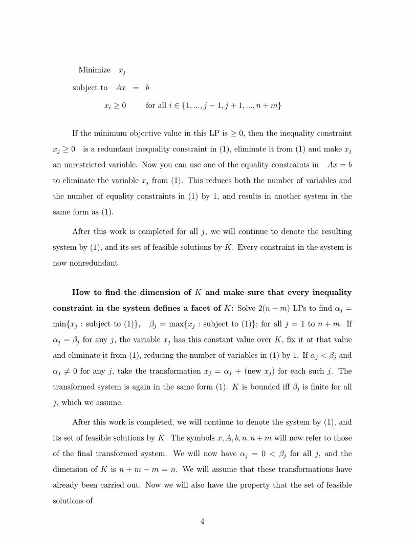
Minimize xj

subject to Ax = b

xi ≥ 0 for all i ∈ 1, ..., j − 1, j + 1, ..., n+m

If the minimum objective value in this LP is ≥ 0, then the inequality constraintxj ≥ 0 is a redundant inequality constraint in (1), eliminate it from (1) and make xj

an unrestricted variable. Now you can use one of the equality constraints in Ax = b

to eliminate the variable xj from (1). This reduces both the number of variables and

the number of equality constraints in (1) by 1, and results in another system in the

same form as (1).

After this work is completed for all j, we will continue to denote the resulting

system by (1), and its set of feasible solutions by K. Every constraint in the system is

now nonredundant.

How to find the dimension of K and make sure that every inequality

constraint in the system defines a facet of K: Solve 2(n+m) LPs to find αj =

minxj : subject to (1), βj = maxxj : subject to (1); for all j = 1 to n +m. If

αj = βj for any j, the variable xj has this constant value over K, fix it at that value

and eliminate it from (1), reducing the number of variables in (1) by 1. If αj < βj and

αj = 0 for any j, take the transformation xj = αj + (new xj) for each such j. The

transformed system is again in the same form (1). K is bounded iff βj is finite for all

j, which we assume.

After this work is completed, we will continue to denote the system by (1), and

its set of feasible solutions by K. The symbols x,A, b, n, n+m will now refer to those

of the final transformed system. We will now have αj = 0 < βj for all j, and the

dimension of K is n +m −m = n. We will assume that these transformations have

already been carried out. Now we will also have the property that the set of feasible

solutions of

4

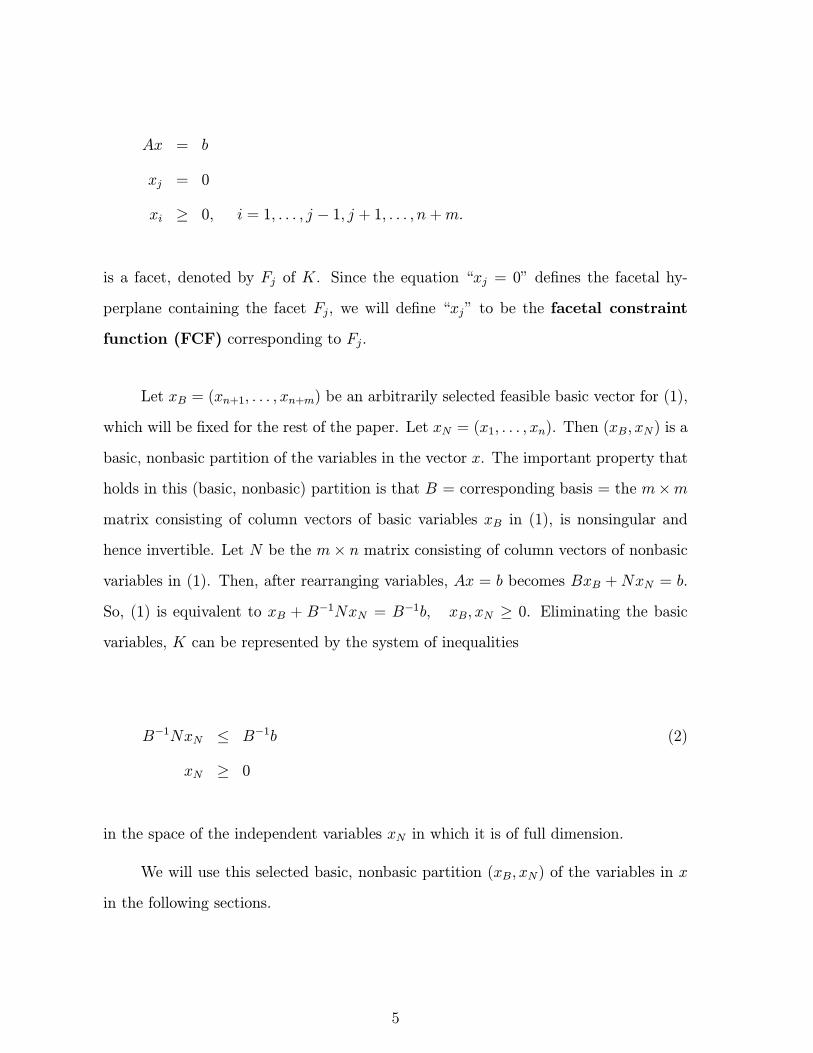
Ax = b

xj = 0

xi ≥ 0, i = 1, . . . , j − 1, j + 1, . . . , n+m.

is a facet, denoted by Fj of K. Since the equation “xj = 0” defines the facetal hy-

perplane containing the facet Fj, we will define “xj” to be the facetal constraint

function (FCF) corresponding to Fj.

Let xB = (xn+1, . . . , xn+m) be an arbitrarily selected feasible basic vector for (1),

which will be fixed for the rest of the paper. Let xN = (x1, . . . , xn). Then (xB, xN) is a

basic, nonbasic partition of the variables in the vector x. The important property that

holds in this (basic, nonbasic) partition is that B = corresponding basis = the m×mmatrix consisting of column vectors of basic variables xB in (1), is nonsingular and

hence invertible. Let N be the m× n matrix consisting of column vectors of nonbasicvariables in (1). Then, after rearranging variables, Ax = b becomes BxB +NxN = b.

So, (1) is equivalent to xB + B−1NxN = B−1b, xB, xN ≥ 0. Eliminating the basic

variables, K can be represented by the system of inequalities

B−1NxN ≤ B−1b (2)

xN ≥ 0

in the space of the independent variables xN in which it is of full dimension.

We will use this selected basic, nonbasic partition (xB, xN) of the variables in x

in the following sections.

5

2 Historical Note

Extreme points of convex polyhedra were brought to prominence by George Dantzig

when he introduced the simplex method for solving linear programs in 1947 [3]. This

work of his is perhaps the most fundamental contribution in the annals of the study of

convex polyhedra. Until then work on them remained the domain of abstract thinkers

and their imagination. His work brought a new computational dimension to the study

of convex polyhedra [9, 4].

Until Dantzig’s work, visualization was only possible for 2-dimensional polyhedra.

When you draw the picture of a 2-dimensional polyhedron, you can see (i.e., visualize)

the adjacent extreme points of each extreme point, and thus get a “visual”-feel of the

neighborhood of each of its extreme points. In higher dimensional polyhedra, we can

do the same through computation using the primal simplex pivot steps. Thus, the

techniques that originated in Dantzig’s simplex method (in particular the wonderful

computational tool of the primal simplex pivot step; and Phase I of the primal simplex

method, the extension of the classical Gauss-Jordan method developed by the Chinese

and Indians many centuries ago for solving linear equations into a method for solving

linear inequalities) made it possible to compute any portion of a convex polyhedron

that we want to see and visualize. One of the most important outcomes of Dantzig’s

work for mathematics is to bring about the possibility of clear visualization to convex

polyhedra of dimension ≥ 3 through computation [9].

I will mention three example problems. On 2-dimensional polyhedra, answers

to each of these three example problems can be found quickly and visually. In higher

dimensions the same thing can be done through computation by solving a small number

of linear and convex quadratic programming problems, illustrating this “visualization

through computation”: (1): Given a polytope Q specified through a system of linear

inequalities in n variables, suppose we want to see whether Q is nonempty, and if it is

nonempty see what its dimension is. All this can be accomplished through computation

by solving a small number of linear programs. (2): Given a polytope P of full dimension

6

in Rn specified through a system of linear inequality constraints, and a hyperplane H

intersecting P specified by a linear equation, suppose we want to “see” how far H can

move either left or right while still keeping a nonempty intersection with P . In each

direction, this can be seen through computation by solving a single linear program.

(3): Suppose we are given a subset S of extreme points of P . Suppose we want to

“see” whether S is the set of all extreme points of P , and if not obtain an extreme

point of P not in S. The algorithm discussed in this paper allows us to do that through

computation, by solving a small number of linear and convex quadratic programs when

K belongs to Class 2 defined in Section 8.

Ever since his work in 1947, the problem of enumerating all the extreme points of

a convex polytope specified by linear constraints has been recognized as an important

one.

There are several algorithms for this problem already, most of them are based on

enumerating the feasible bases for (1), or faces of K of all dimensions. Public software

programs implementing these algorithms are also available. But in all these algorithms,

after computing r extreme points, the effort needed to compute the next one grows

exponentially with r in the worst case.

An algorithm for this problem is said to be an efficient algorithm, or polynomial

time algorithm, if it satisfies the following properties:

1. It should obtain the extreme points of K sequentially one after the other in a

list.

2. When the list of known extreme points of K, d1, . . . , dr, contains r extremepoints, the effort needed in the algorithm to check whether it contains all the

extreme points of K, and if it does not, to generate a new extreme point, should

be bounded above by a polynomial in r and the size of system (1).

The goal of developing an efficient algorithm for this problem is more of a math-

ematical challenge, than a practical one. We will address this mathematical challenge.

7

The algorithm that we develop is based on solving a series of linear programs and

convex quadratic programs , and checking the dimension of the optimal faces of some

of the linear programs solved, which in turn requires solving more linear programs as

discussed above. Proof of the polynomial time property of the algorithm is based on the

well known fact that LPs and convex QPs can be solved by polynomial time algorithms.

The reason why the proposed algorithm may not be practical while maintaining its

polynomial time property, is its reliance on polynomial time algorithms for LP, convex

QP which have not proven to be practical.

For the special case when (1) is the system of constraints in a pure network flow

problem, Proven [10] has developed an efficient algorithm for this problem using the

special properties of node-arc incidence matrices. We consider the case of general linear

constraints.

In [5], the authors proved that the problem of enumerating all the extreme points

of an unbounded convex polyhedron specified by linear constraints is hard, but the

problem remains open if the polyhedron is bounded, i.e., if it is a polytope. We will

consider this case, i.e., assume that K is a polytope in the sequel. Also, for the sake

of simplicity, we will assume that exact arithmetic is used.

3 Relationship Between the Problems of Enumer-

ating Extreme Points, and Facets

Consider a convex polytope P of dimension n in Rn. There are two different ways of

representing it algebraically. These are:

1. Convex hull representation: Let x1, . . . , x be the set of all extremepoints of P . Then P = < x1, . . . , x >, the convex hull of its set of extreme points.

8

2. Halfspace intersection representation: P can be represented as the

intersection of a finite number of halfspaces of Rn (i.e., as the set of feasible solutions

of a system of linear inequalities).

These two different representations lead to two different enumeration problems

associated with P . They are:

Extreme point enumeration problem: When P is given in halfspace in-

tersection representation (i.e., as the set of feasible solutions of a system of linear

inequalities), enumerate all the extreme points of P .

Facet enumeration problem: When P is given as the convex hull of its ex-

treme points, enumerate all the facetal inequalities to represent it as the set of feasible

solutions of a system of linear inequalities.

In the theory of convex polytopes, these two problems are known as the duals

of each other. An algorithm for one of these problems can be used to solve the other

problem directly. To show this, we denote by:

Procedure A: Any algorithm for enumerating the extreme points of P when it is

specified as the set of feasible solutions of a nonredundant system of linear inequalities

of full dimension.

Procedure B: Any algorithm for enumerating all the facetal inequalities to

represent P when it is given as the convex hull of its extreme points.

How to enumerate all the facetal inequalities to represent P when the

set of its extreme points x1, . . . , x is given, using Procedure A

We assume that each xt is an extreme point of P = < x1, . . . , x > of full

9

dimension n. Let x = (x1 + . . .+ x )/ , an interior point of P .

Take the transformation x = y + x, let yt = xt − x for t = 1 to . Then

P = < x1, . . . , x > = < y1, . . . , y > +x. Also 0 is an interior point of< y1, . . . , y >.

Let q = (q1, . . . , qn) be a row vector of variables in Rn. Use Procedure A to

generate all the extreme points of the polytope in q-space defined by the inequalities

qyt ≤ 1, t = 1 to . Let q1, . . . , qM be the set of extreme points of this polytope.Then

< y1, . . . , y > = y : qsy ≤ 1, s = 1, ...,M

So, in terms of the space of variables x ∈ Rn in which all the extreme points ofthe original P are specified,

P = < x1, . . . , x > = x : qsx ≤ 1 + qsx, s = 1, ...,M

with each inequality being a facetal inequality for P .

How to enumerate all the extreme points of P = x : Qx ≤ h usingProcedure B

Let Q be of order m × n. Assume that P is of full dimension and that each

constraint in its representation given is nonredundant, i.e., that each inequality in this

representation of P corresponds to a facet of P , and that the dimension of P is n. Find

an interior point x of P by using the Low dimension step in Murty & Chung [8] (also

discussed in the next section) to generate extreme points of P until the convex hull

of generated extreme points is of full dimension. Take the transformation x = y + x.

Then P = y : Qy ≤ h−Qx+ x. Also, since x is an interior point of P , h−Qx > 0.For each i = 1 to m, define ai = Qi.(1/(hi −Qi.x)) where Qi. is the i-th row vector ofQ. Therefore P = y : aiy ≤ 1, i = 1, ...,m+ x.

Use Procedure B to generate a linear inequality representation of < a1, . . . , am >.

Suppose it is a : adr ≤ 1, r = 1, ..., L.

10

Then d1, . . . , dL is the set of extreme points of y : aiy ≤ 1, i = 1, ...,m.

So, the set of extreme points of P is d1 + x, . . . , dL + x.

Here we will study the extreme point enumeration problem.

4 Key Facts Relating a Convex Polytope and Its

Dual Polytope

The basic references on the properties of the dual polytope of a convex polytope, and

on the relationships between the two of them are Grunbaum [4] in its latest edition,

and Ziegler [12]. But here we will summarize the main facts that we will use in this

paper.

The standard term dual polytope is called polar polytope in [12] and some

other books; and they call the duality relationship between a polytope and its dual

polytope as polarity. We will use the terms, dual polytope and duality, in this paper.

We consider a general polytope P of dimension n with 0 in its interior, represented

by the system of inequalities

At.x ≤ 1 t = 1 to M

in x ∈ Rn, in which each inequality is nonredundant. Let x1, ..., xN be the set of allits extreme points. Then its dual polytope Q in the space of variables a ∈ Rn (here ais a row vector) is the set of feasible solutions of

axt ≤ 1 t = 1, ..., N

and A1., ..., AM. is the set of all extreme points of Q. So, among the polytopesP,Q; extreme points of one of them are in one-to-one correspondence with facets (i.e.,

coefficient vectors of FCFs) of the other.

11

Also, let F be any nonempty proper face of P . Suppose x1F , ..., xsF is the set ofall extreme points of F . Let H be the face of Q defined by the system

axiF = 1 i = 1, ..., s

axt ≤ 1 for all xt ∈ x1, ..., xN\x1F , ..., xsF

Then H is said to be the face of Q corresponding to the face F of P . It can be

verified that this correspondence between faces of P,Q is one-to-one. So, among P,Q

every nonempty proper face of one of them corresponds to a unique nonempty proper

face of the other under this correspondence. Also, the following relationship can be

verified to hold:

(the dimension of a nonempty proper face of P ) + (the dimension of the

cooresponding face of Q) = n− 1.

For any face F of P let ψ(F ) denote the face of Q corresponding to F . Here is

another important property.

Inclusion-reversing property: If F,G are two faces of P satisfying F ⊂G, then ψ(F ) ⊃ ψ(G).

We will now derive a theorem that we will use in the proofs in Section 8.

Theorem 4.1: Consider the pair of extreme points xt, xs of P ; and the facets

ψ(xt),ψ(xs) of Q corresponding to them. Let ∆(xt, xs) denote the smallest dimensional

face of P containing both xt, xs. Then ψ(∆(xt, xs)) = ψ(xt) ∩ ψ(xs).

Proof: It is possible that there is no facet of P containing both xt, xs. In this

case ∆(xt, xs) = P itself. In this case the face of Q corresponding to ∆(xt, xs) = P

12

is the empty face ∅. Also, verify that ψ(xt) ∩ ψ(xs) = ∅, so the result in the theoremholds for this case.

Now consider the case in which there is at least one facet of P containing both

xt, xs. Let F1, ..., Fr be all the facets of P that contain both the extreme points xt

and xs. Then ∆(xt, xs) = ∩ri=1Fi. By the properties mentioned above, we see thatψ(F1), ...,ψ(Fr) are all the extreme points of Q contained in both its facets ψ(x

t) and

ψ(xs), so ψ(xt)∩ψ(xs) is the convex hull < ψ(F1), ...,ψ(Fr) >. Again, by the aboveproperties we see that the face of P corresponding to the face ψ(xt) ∩ ψ(xs) of Q is

∩ri=1Fi = ∆(xt, xs).

5 Segments and Their Properties

Murty and Chung [8] introduced the concept of a segment of a polytope and used it

to enumerate its extreme points and faces. They defined segments of various orders

ranging from 1 to (−2 + the dimension of the polytope). Here we will only use segmentsof order 1, and hence we will refer to segments of order 1 as segments.

Definition 5.1: (Segment): A segment of a convex polytope K of dimension

n is the convex hull, E, of a subset of its extreme points satisfying: (i) its dimension

is the same as that of K, n, (ii) adjacency of extreme points on E coincides with that

on K (i.e., every edge of E is also an edge of K).

In [8] the following two steps, LD and NS-1, have been developed for our problem

(these names for the steps are new, these names have not been used in [8]).

LD (Low Dimension Step): Let Γ = < d1, . . . , dr > be the convex hull of

the present list of known extreme points of K. If dimension(Γ) < dimension(K), find

the equation for a hyperplane containing Γ, in the space of the variables xN in which

K has full dimension. To do this, for k = 1 to r, let (dkB, dkN ) be the partition of the

13

vector dk according to (xB, xN) partition selected in Section 1 for the variables x.

The dimension of d1, . . . , dr is the rank of the set of vectors dkN − d1N : k =2, . . . , r.

If this dimension is < n, the following homogeneous system of linear equations in

variables fN (written as a row vector)

fN(dkN − d1N) = 0, k = 2, . . . , r

has a nonzero solution fN = 0, find it. Let β = fNd1N . Then all the extreme points

d1, . . . , dr lie on the hyperplane represented by the equation fNxN = β in the space of

the independent variables xN .

Now solve the two LPs, minimize fNxN , and maximize fNxN subject to (1). One

or both of these LPs will have as an optimum extreme point a point not in the current

list. Call it dr+1, add it to the list.

The application of the LD step can be repeated until the dimension of Γ = <

d1, . . . , dr >, the convex hull of the present list of known extreme points of K, becomes

= n = dimension of K. Once the dimension of Γ becomes = n, some new steps are

needed to generate additional extreme points of K. One of these is the NS-1 step

described next.

NS-1 (Non-Segment-1 Step): Let Γ = < d1, . . . , dr > be the convex hull of

the present list of known extreme points ofK satisfying dimension(Γ) = dimension(K).

Let p = (p1, . . . , pn+m)T , q = (q1, . . . , qn+m)

T be a pair of extreme points of K.

They are adjacent on K iff rank of A.j : j such that either pj or qj or both are > 0is −1 + (its cardinality), nonadjacent on K iff the rank of this set is < −1 + (its

cardinality).

p, q are adjacent on Γ = < d1, . . . , dr > iff the following system in variables

c = (c1, . . . , cn+m) has a feasible solution, which can be checked by solving an LP.

14

c(p− q) = 0

c(p− dk) > 0, for all k such that dk = p or q. (3)

If a pair of extreme points of Γ; p, q say; which are adjacent on Γ, are not adjacent

on K, then from the vector c satisfying (3); we get the supporting hyperplane cx = cp

of Γ that contains only extreme points p, q but no other extreme point of Γ, which is

not a supporting hyperplane for K.

Now solve the LP: maximize cx overK to get an extreme point optimum solution.

That extreme point may be a new extreme point of K not in the present list, but it

could also be p or q itself. If it is a new extreme point of K not in the present list, add

it to the list, and apply this NS-1 step again. If it is p or q, let cp = γ, now p, q are the

only extreme points of K known at present on the face S of K determined by

Ax = b

cx = γ

x ≥ 0

Therefore by applying the LD step on S a new extreme point of K on S not in

the present list can be determined in this case, add it to the list.

The application of NS-1 can be continued until at some stage the convex hull of

the present list becomes a segment of K. To continue the enumeration then, some new

steps are needed. One of those is LDF-1 given below.

LDF-1 (Low Dimension Facet Intersection Step): Let Γ = < d1, . . . , dr >

be the convex hull of the present list of known extreme points of K which is a segment

15

of K. If there is a facet F of K satisfying dimension(F ∩ Γ) < dimension(F ), apply

the LD step on F and obtain a new extreme point of K on F and add it to the list.

The application of Steps NS-1, LDF-1 can again be continued until at some stage

the conditions in the following definition hold for the extreme points in the present list

(mukka is taken from a Telugu word meaning “a piece of an object which displays all

the important properties of the orginal”).

Definition 5.2 (Mukka): A mukka of a convex polytope K is the convex hull

of a subset of extreme points of K which is a segment of K that has a full dimensional

intersection with every facet of K.

When the convex hull of the present list of extreme points of K becomes a mukka

of K, to continue the enumeration efficiently, some new steps are needed. These are

discussed in the next section.

6 The Dual Polytope Step, to Continue the Enu-

meration

Let Γ = < d1, . . . , dr > be the convex hull of the present list of known extreme

points of K which is a mukka of K. Here we will discuss how to use the dual polytope

of Γ to continue the enumeration of extreme points of K at this stage. For details on

dual polytopes of convex polytopes, see Section 4 and [4, 12]. I believe this is the first

algorithmic use of the dual polytope of a convex polytope.

Cautionary note: The duality that we discuss in this paper refers is the duality

between a convex polytope and its dual polytope mentioned in Section 4; not the

“duality between linear programs” discussed in LP books.

16

The original polytope K in the space of nonbasic variables xN = (x1, . . . , xn)T

selected in Section 1, has the representation

−IxN ≤ 0 (4)

B−1NxN ≤ B−1b

where I is the unit matrix of order n.

Let d = (d1 + . . . + dr)/r. The points d1, . . . , dr, d correspond to d1N , . . . , drN , dN

in the space of nonbasic variables xN . Translating the origin to d, i.e., taking the

transformation x = y + d, in the space of independent variables yN = (y1, . . . , yn)T , Γ

becomes dN+ < y1N , . . . , y

rN >; where y

t = dt − d = (yt1, . . . , ytn+m), ytN = (yt1, . . . , ytn)T

for t = 1 to r, and dN = (d1, . . . , dn)T .

Carrying out the same transformation x = y + d on (4), we see that the repre-

sentation of y = x− d : x ∈ K in the space of the yN is

−IyN ≤ dN (5)

B−1NyN ≤ B−1b−B−1NdN

Also, since 0 is an interior point of< y1, . . . , yr >, we know that β = (β1, . . . , βm)T =

B−1b − B−1NdN > 0, and dN = (d1, . . . , dn)T > 0. So, by dividing each constraint in(5) by its RHS constant and denoting the row vectors qi = (−Ii.)/di for i = 1 to n,

and qn+i = (B−1N)i./βi for i = 1 to m, we can express (5) in the form (6) given below:

qiyN ≤ 1 for i = 1 to n+m (6)

17

In this representation of K in the space of the variables yN , qiyN is the FCF

for the facet Fi corresponding to the i-th constraint in (6), and the vector qi is its

coefficient vector, it is known as the FCF coefficient vector corresponding to Fi

in this representation. So, y1N , . . . , yrN is the present set of known extreme pointsolutions of (6), and < y1N , . . . , y

rN > is a mukka for the set of feasible solutions of (6).

From Sections 3, 4 we know that a1y1 + . . . + anyn ≤ 1 represents a facet for

< y1N , . . . , yrN > iff a = (a1, . . . , an) is an extreme point solution of the system in

variables a

aytN ≤ 1 for t = 1 to r (7)

The set of feasible solutions of (7), Ω, is the dual polytope of Γ= < y1N , ..., yrn >,

see Section 4 and [4, 12]. Every extreme point of Ω is the FCF coefficient vector in an

inequality constraint with RHS constant 1 in a constraint representation of Γ.

When Γ is a mukka of K; the FCF coefficient vectors for K in its representation

(6) (the points q1, . . . , qn+m) are extreme point solutions of (7). Extreme points of (7)

outside of the set q1, . . . , qn+m correspond to facets of Γ whose facetal hyperplanesare not facetal hyperplanes of K.

If < q1, . . . , qn+m > is not a mukka for the set of feasible solutions of (7) in the

space of variables a, then the LD, NS-1, LDF-1 steps discussed in Section 5 can be

applied to generate a new extreme point solution p for (7) which is not in the set

q1, ..., qn+m. Then pyN ≤ 1 represents a new facet for < y1N , . . . , yrN > that does

not correspond to a facet of the original polytope K. In this case an extreme point

solution for the problem of maximizing pxN subject to (2), or (1) would lead to a new

extreme point dr+1 for the original polytope K; add it to the list and then continue

the enumeration of extreme points of K as in Section 5 again.

18

7 Mukkadvayams for K

The procedures discussed in Sections 5, 6, can help us to enumerate the extreme points

of K until we get Γ = < d1, . . . , dr > = the convex hull of the present list of known

extreme points of K satisfying the following properties 1 and 2.

1. Γ is a mukka of K.

2. Let d = (d1 + . . . + dr)/r; yt = dt − d for t = 1 to r; β = (β1, . . . ,βm)T =

B−1b − B−1NdN ; qi = (−Ii.)/di for i = 1 to n, and qn+i = (B−1N)i./βi for i

= 1 to m. Then q1, . . . , qn+m, the set of FCF coefficient vectors of K in its

representation (6) in the space of variables yN , is a mukka for the set of feasible

solutions Ω of the following system in variables a = (a1, . . . , an)

aytN ≤ 1 for t = 1 to r (8)

Definition (Mukkadvayam) 7.1: At this stage when Γ satisfies both Properties

1 and 2 stated above, we will call it a mukkadvayam of K (dvayam is another Telugu

word meaning pair, this name refers to the fact that not only is Γ a mukka of K at

this stage, but < q1, . . . , qn+m >, the convex hull of the FCF coefficient vectors in

(6) defining K, is a mukka of the dual polytope Ω of Γ). Likewise, at this stage,

< q1, . . . , qn+m > is a mukkadvayam of Ω.

It can be verified that until this stage, the enumeration is efficent. To continue

the enumeration beyond this stage efficiently, some new steps are needed. At this stage,

a face G of K is said to be

• a complete face of K for mukka Γ if G ∩ Γ = G

• an incomplete face of K for mukka Γ if G ∩ Γ = G

19

• a star face of K for mukka Γ if dimension(G ∩ Γ) < dimension(G).

Also, at this stage a row vector p = (p1, . . . , pn) which is an extreme point of Ω

not contained in q1, . . . , qn+m is said to be

• a star DPEP (dual polytope extreme point) vector for Γ at this stage.

When Γ = K, there exist faces of K which are star faces for Γ (in fact every edge

of K incident at an extreme point of K which is not in Γ, is a star face for Γ); and also

star DPEP vectors for Γ (in fact if no star DPEP vector for Γ exists, then q1, . . . , qn+m

are the only extreme point solutions for (8), which implies that Γ corresponds to the

set of feasible solutions of (6), i.e., that Γ = K).

If a star face E of K for Γ can be found, then by applying the LD step on E

for the known set d1, . . . , dr ∩ E of extreme points on it, a new extreme point of

E not in Γ can be found efficiently. Likewise if a star DPEP vector p for Γ can be

found, then by maximizing pxN over K, a new extreme point of K not in Γ can be

found. Hence efficient enumeration of extreme points becomes possible, if an efficient

procedure can be developed to find either a star face of K with respect to the set of

known extreme points of K, or a star DPEP vector for it. In fact in the process of

generating a mukkadvayam for K, Steps NS-1, LDF-1 of Section 5 find and use star

faces of K for the current set of extreme points Γ; and the dual polytope step of Section

6 finds and uses star DPEP vectors for Γ, to find a new extreme point of K not in Γ.

The central problem in enumerating extreme points efficiently: Given

Γ, a mukkadvayam of K, develop a procedure for identifying a star face of K for Γ, or

a star DPEP vector for Γ efficiently, or show that neither of them exist.

8 Mukkadvayam Checking Step

Note On this Section

20

In this section we will discuss the next step. We keep on applying this step as

long as it is generating new extreme points of K not in the list, and stop using it only

when a full application of it did not yield a new extreme point of K to add to the list.

We also include in this section all the results and their proofs to show that at the end

of this step the Fi = Fi∩Γ for i = 1 to n+m satisfy the property that the dimensions

of Fi ∩Fj and Fi ∩Fj will be the same for all i, j; and a corresponding property holdsfor the dual polytope of Γ.

However, Hans Raj Tiwary [11] constructed a 5-dimensional counterexample to

show that with all the steps developed so far including this mukkadvayam checking

step, the procedure cannot guarantee that Γ = K at termination.

We will classify polytopes of dimension n in Rn into two classes:

Class 1: The polytope K belongs to this class if it has at least one extreme point

yN , and a hyperplane H through yN , such that every facet of K incident at yN has

relative interior point intersection with both sides of H.

Class 2: The polytope K belongs to this class if every hyperplane through any

extreme point ofK contains at least one facet ofK incident at that extreme completely

on one of its sides.

In Section 9 following this section we discuss the final step, and show in Section 10

that if the polytopeK belongs to Class 2, then even without applying the mukkadvayam

checking step of this section, the earlier steps together with the final step guarantee that

all extreme points of K will be enumerated. In spite of this, the reason for including

this mekkadvayam checking step and all the results on what can be guaranteed with

it; is that I believe that when the mukkadvayam checking step is also included, all the

extreme points of K can be guaranteed to be enumerated even when K belongs to

Class 1. I do not have a proof of this yet.

Γ, the convex hull of the present list of extreme points of K, is a mukkadvayam

21

when we come to this step. The work described in this section is based on a single

procedure. In this step this procedure is applied on the dual polytope Ω of Γ, and on

the original polytope K. We describe the application of this procedure on Ω, and on K

separately below for clarity. If there are extreme points of K which are not in Γ, then

these procedures may output a new extreme point of K not in Γ, we then add it to the

list of extreme points generated, and go back to Section 5 to convert the augmented Γ

into a mukkadvayam again.

Procedure on Ω

Let Γ = < y1N , . . . , yrN > = the convex hull of the present list of known extreme

points of K in its representation (6) in the space of variables yN , be a mukkadvayam

of K. This is one step for checking whether Γ = K, if not this step may produce a

new extreme point of K not in Γ. If a new extreme point is generated, we go back to

Section 5 again to convert the new set of extreme points into a mukkadvayam again.

For a pair t, s in 1, ..., r, define the following (in the LPs given, the variablesare a = (a1, . . . , an), the variables in (7) defining the dual polytope Ω of Γ).

μts(Ω) = Minimum value of aysN

subject to aytN = 1

aywN ≤ 1 for w ∈ 1, . . . , t− 1, t+ 1, . . . , r

Uts(Ω) = optimum face of the above LP defining μts(Ω)

22

νts(Ω) = Maximum value of aysN

subject to aytN = 1 (9)

aywN ≤ 1 for w ∈ 1, . . . , t− 1, t+ 1, . . . , r

Vts(Ω) = optimum face of the above LP defining νts(Ω)

μts(q1, . . . , qn+m) = minaysN : a ∈ qi : i = 1, . . . , n+m s. th. qiytN = 1

Uts(q1, . . . , qn+m) = convex hull of all the a that tie for the minimum defining

μts(q1, . . . , qn+m)

νts(q1, . . . , qn+m) = maxaysN : a ∈ qi : i = 1, . . . , n+m s. th. qiytN = 1(10)

Vts(q1, . . . , qn+m) = convex hull of all the a that tie for the maximum defining

νts(q1, . . . , qn+m)

If μts(Ω) < μts(q1, . . . , qn+m) [or νts(Ω) > νts(q1, . . . , qn+m)], then an ex-treme point optimum solution for the LP defining μts(Ω) [νts(Ω)] will lead to a star

DPEP vector for Γ.

A note on checking the dimension of Vts(Ω): The optimum face of a lin-

ear program is always a face of its set of feasible solutions. For an LP like (9), the

system of constraints characterizing its optimum face is obtained from the system of

constraints in (9) by changing some of the inequalities in it into equations. When (9) is

solved, the complementary slackness optimality conditions in LP theory clearly identify

which inequality constraints in (9) must be changed into equality constraints to get

its optimum face. Then the dimension of this optimum face can be checked using the

procedure discussed at the beginning of this paper.

23

If μts(Ω) = μts(q1, . . . , qn+m), but dimension(Uts(Ω)) > dimension(Uts(q1, . . . ,qn+m)), then Uts(Ω) is a star face of Ω for its mukka q1, . . . , qn+m. If νts(Ω) =νts(q1, . . . , qn+m), but dimension(Vts(Ω)) > dimension(Vts(q1, . . . , qn+m)), thenVts(Ω) is a star face of Ω for its mukka q1, . . . , qn+m. In either of these cases, byapplying the LD step on this star face for Ω we can find an extreme point of Ω not in

q1, . . . , qn+m, which leads to a star DPEP vector for Γ.

If a star DPEP vector p has been found, then find an an extreme point solution

for the problem of maximizing pxN subject to (2), or (1); this will lead to a new extreme

point dr+1 of the original polytope K not in the current list; add it to the list and then

continue the enumeration of extreme points of K as in Section 5 again.

If μts(Ω) = μts(q1, . . . , qn+m), νts(Ω) = νts(q1, . . . , qn+m), dimension( Uts(Ω))= dimension(Uts(q1, . . . , qn+m)), and dimension(Vts(Ω)) = dimension( Vts(q1,. . . ,qn+m)) for all t, s; then this procedure has failed to find a star DPEP vector for Γ atthis stage. In this case continue.

Procedure on K

Consider a facet Fi of K defined by the FCF qiyN in its representation (6) in the

space of variables yN . For i ∈ 1, . . . , n +m, the FCF of the facet Fi of K is qiyN .

Γ, Fi∩Γ are available to us as convex hulls of their extreme points. So, in the following,to optimize a linear function on Γ or Fi ∩ Γ, we evaluate the linear function at eachextreme point of the set, and select the best. Define:

24

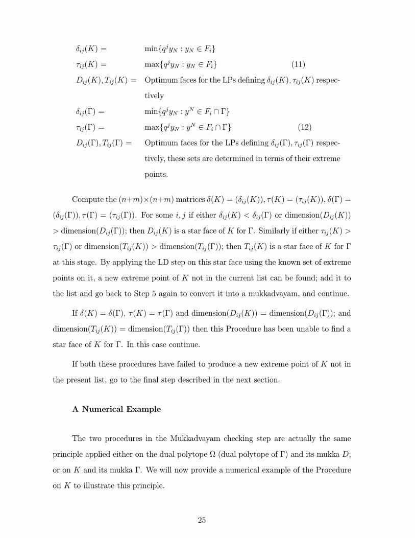
δij(K) = minqjyN : yN ∈ Fiτij(K) = maxqjyN : yN ∈ Fi (11)

Dij(K), Tij(K) = Optimum faces for the LPs defining δij(K), τij(K) respec-

tively

δij(Γ) = minqjyN : yN ∈ Fi ∩ Γτij(Γ) = maxqjyN : yN ∈ Fi ∩ Γ (12)

Dij(Γ), Tij(Γ) = Optimum faces for the LPs defining δij(Γ), τij(Γ) respec-

tively, these sets are determined in terms of their extreme

points.

Compute the (n+m)×(n+m) matrices δ(K) = (δij(K)), τ(K) = (τij(K)), δ(Γ) =(δij(Γ)), τ (Γ) = (τij(Γ)). For some i, j if either δij(K) < δij(Γ) or dimension(Dij(K))

> dimension(Dij(Γ)); then Dij(K) is a star face of K for Γ. Similarly if either τij(K) >

τij(Γ) or dimension(Tij(K)) > dimension(Tij(Γ)); then Tij(K) is a star face of K for Γ

at this stage. By applying the LD step on this star face using the known set of extreme

points on it, a new extreme point of K not in the current list can be found; add it to

the list and go back to Step 5 again to convert it into a mukkadvayam, and continue.

If δ(K) = δ(Γ), τ(K) = τ (Γ) and dimension(Dij(K)) = dimension(Dij(Γ)); and

dimension(Tij(K)) = dimension(Tij(Γ)) then this Procedure has been unable to find a

star face of K for Γ. In this case continue.

If both these procedures have failed to produce a new extreme point of K not in

the present list, go to the final step described in the next section.

A Numerical Example

The two procedures in the Mukkadvayam checking step are actually the same

principle applied either on the dual polytope Ω (dual polytope of Γ) and its mukka D;

or on K and its mukka Γ. We will now provide a numerical example of the Procedure

on K to illustrate this principle.

25

Example: Here we illustrate the application of the above Procedure on a poly-

tope K ⊂ R4 defined by the constraints

ai(x) = ai1x1 + ai2x2 + ai3x3 + ai4x4 ≤ 1, i = 1, . . . , 15

where (ai1, ai2, ai3, ai4) : i = 1 to 15 = (1, 1, 1,−1), (1, 1,−1, 1), (1, 1,−1,−1),(1, ,−1, 1, 1), (1,−1, 1,−1), (1,−1,−1, 1), (1,−1, −1,−1), (−1, 1, 1, 1), (−1, 1, 1, −1),(−1, 1,−1, 1), (−1, 1,−1,−1), (−1,−1, 1, 1), (−1,−1, 1,−1), (−1,−1,−1, 1), (−1,−1,−1,−1). Here K is defined by a general system of linear constraints, which is not in

standard form.

Let I denote the unit matrix of order 4. It can be verified that Γ = convex hull

of I.j,−I.j : j = 1 to 4 is a mukka of K.

Let Ft be the facet of K on the facetal hyperplane defined by at(x) = 1, for t =

1 to 15. at(x) is the FCF corresponding to Ft for t = 1 to 15.

Consider the problem of maximizing a2(x), the FCF of F2, on F1 and on F1∩Γ =< I.1, I.2, I.3,−I.4 >. The optimum objective value is 1 in both problems, but the

dimension of the optimum face on F1 is 2; while on F1 ∩ Γ, it is only 1. This showsthat F1 is an incomplete facet of K for Γ. A similar argument shows that the facets

F4 and F8 are also incomplete facets of K for Γ.

Results on the Output Obtained By the Procedure Using Steps Dis-

cussed So Far

Let Γ = < y1N , . . . , yrN > = the convex hull of the present list of known extreme

points of K in its representation (6) in the space of variables yN , be a mukkadvayam

of K, and suppose Γ is not = K. Then every facetal hyperplane of K is also a

facetal hyperplane of Γ, but Γ must have some additional facetal hyperplanes which

are not facetal hyperplanes of K; these additional facetal hyperplanes of Γ are called its

non-K-facetal hyperplanes, and facetal hyperplanes of K are called the K-facetal

hyperplanes of Γ. Also, the facets of Γ on these respective facetal hyperplanes are

26

called its non-K- facets, K-facets respectively. Remember in this case both Γ and

K\Γ have dimension n.

In the same way any face of Γ which is also a face of K is called a K-face of

Γ, faces of Γ which are not faces of K are called non-K-faces of Γ. Let G be any

non-K-facet of Γ. The following results can easily be verified at this stage.

1. There is an n-dimensional portion of K\Γ on the side of the facetalhyperplane corresponding to G not containing Γ, and the n-dimensional Γ

on the other side.

2. Every non-K-facetal hyperplane of Γ has the property that all of Γ lies

on one side of it, and an n-dimensional portion of K\Γ lies on the otherside. This implies that a non-K-facet of Γ can never be a subset of a facet

of K.

3. Since Γ is a mukka of K, all its vertices and edges, are vertices and edges

of K. So the set of edges in any non-K-facet of Γ is a union of the sets of

edges in several faces of K.

4. Since Γ is a mukka ofK, the introduction of the inequality corresponding

to G in the system of inequalities representing Γ, does not create any new

extreme points, edges which are not extreme points, edges of K.

Let T be a face of K of dimension d, such that T ∩G = ∅, and T ⊂ G. SinceΓ is a segment of K, when d = 1 or 2, T ∩G must be a lower dimensionalboundary face of T . When d ≥ 3, there are two possibilities: (a) either

T ∩ G is a lower dimensional boundary face of T , or (b) T contains d-

dimensional portions on both sides of the facetal hyperplane corresponding

to G.

Also, if T is a face of K of dimension 1 , and T ∩Γ consists of more than asingle extreme point of T ; or if T is of dimension 2 and T ∩ Γ is more thana single extreme point or single edge of T ; then T must be a subset of Γ,

i.e., it must be a face of Γ.

27

5. Suppose a facet Fp of K has an intersection with G, which is an (n −2)−dimensional face ofK. Then Fp∩Gmust be a facet of Fp, so, Fp is on oneside of G. But since Γ is a mukka, this implies that Fp must be completely

in Γ. But since K\Γ is n-dimensional, we again have a contradiction. Thisimplies that any K-face of G must have dimension ≤ n− 3.

6. Suppose there is a d-dimensional face T of K which has d-dimensional

portions on both sides of G with the property that T ∩ G has a (d − 2)-dimensional face W of T . From properties 4 and 5, we know that 3 ≤ d ≤(n−1); and since T has d-dimensional portions on both sides of G, W must

be a common boundary facet of two facets of T , one lying on the Γ-side of

G, and the other lying on the other side.

The following definitions and properties are used in deriving the results. For all

i = 1 to n+m, Fi denotes the facet of Γ that is a subset of the facet Fi of K.

Definition 8.1: For any pair of extreme points ysN , ytN of Γ, define∆(y

sN , y

tN )

to be the smallest dimensional face of K that contains both ysN and ytN .

Definition 8.2: For any pair of extreme points qi, qj ofD = < q1, ..., qn+m >

define Λ(qi, qj) to be the smallest dimensional face of Ω that contains both

of them.

Property 8.1: For every pair of extreme points ysN , ytN of Γ, ∆(y

sN , y

tN)∩Γ

is the smallest dimensional face of Γ containing both ysN , ytN and it has the

same dimension as ∆(ysN , ytN). Also, if ∆(y

sN , y

tN) has dimension 1 or 2,

then ∆(ysN , ytN) ∩ Γ = ∆(ysN , y

tN), i.e., ∆(y

sN , y

tN) is a K-face of Γ.

Property 8.2: For every pair of extreme points qi, qj of D, Λ(qi, qj) ∩ Dis the smallest dimensional face of D containing both qi, qj, and it has the

same dimension as Λ(qi, qj). Also, if Λ(qi, qj) has dimension 1 or 2, then

Λ(qi, qj) ∩D = Λ(qi, qj), i.e., Λ(qi, qj) is a face of D.

28

Theorem 8.1: Let x, y be any two extreme points of a polytope P . Then the

smallest dimension face of P containing both x, y is unique.

Proof: Let the dimension of a smallest dimension face of P containing both x, y

be d. Suppose P1, P2 are two faces of dimension d both of which contain both x and

y. Then x, y are both contained in the face P1 ∩ P2 of P which is a face of dimension≤ d− 1, contradiction. So, the face of P Containing both x and y is unique.

Theorem 8.2: Let Γ = < y1N , ..., yrN > be a mukkadvayam of K. For some

t, s ∈ 1, ..., r, if the maximum objective value in (9), νts(Ω) is < 1, then the extreme

point ysN of Γ is not contained on any of the facets of Γ incident at ytN , and conversely.

If νts(Ω) = 1, then ysN is contained on a facet of Γ incident at d

t, and conversely.

Proof: Extreme points of Ω defined by (8) are facetal vectors of Γ and vice

versa. From this we see that extreme points of the set of feasible solutions of (9) are

the facetal vectors of facets of Γ incident at ytN . So, νts(Ω) = 1 iff there exists a facetal

vector (a row vector), θ, of a facet of Γ containing ytN , satisfying θysN = 1, but this

shows that ysN satisfies the equation for that facet; hence νts(Ω) = 1 iff there is a facet

of Γ containing both ytN and ysN .

The same argument shows that νts(Ω) < 1 iff ysN is not contained on any of the

facets of Γ incident at ytN .

Theorem 8.3: For any t, s ∈ 1, ..., r, νts(q1, . . . , qn+m), the maximum ob-

jective value in (10), is = 1 iff ysN is contained on a K-facet of Γ incident at ytN .

νts(q1, . . . , qn+m) < 1 iff ysN is not contained on a K-facet of Γ incident at ytN .

Proof: Follows from the arguments in the proof of Theorem 8.2, and the fact

that q1, . . . , qn+m is the set of all FCF coefficient vectors corresponding to K-facetsof Γ in the representation of K in (6)

29

Theorem 8.4: Suppose there exists vertices ytN , ysN of Γ such that ysN is not

contained on any K-facet of Γ incident at ytN , but contained in a non-K-facet of Γ

incident at ytN . Then ∆(ysN , y

tN) = K is not a subset of Γ; and in this case νts(Ω) >

νts(q1, . . . , qn+m), so the Procedure on Ω in the Mukkadvayam checking step outputs

a star DPEP vector for Γ.

Proof: Here ysN is an extreme point of Γ incident to a non-K-facet of Γ incident

at ytN , but not on any of the K-facets of Γ incident at ytN . By Theorems 8.2, 8.3 we

then have νts(Ω) = 1, and νts(q1, . . . , qn+m) < 1. The result in the theorem follows

from this.

Theorem 8.5: Suppose there exists a pair of vertices ytn, ysN of Γ such that: 1.

ysN is contained on some K-facets of Γ incident at ytN , and also at least one non-K-facet

G say, of Γ incident at ytN ; 2. ∆(ytN , y

sN )∩ Γ is not the smallest dimensional face of Γ

containing both ytN and ysN .

Then with these t, s, both νts(Ω), νts(q1, . . . , qn+m) are equal to 1. But the di-mensions of the optimal faces in (9) and (10) are different. So the Procedure on Ω in

the Mukkadvayam checking step outputs a star DPEP vector in this case.

Proof: Let the dimension of ∆(ytN , ysN) be h. Remember that ∆(y

tN , y

sN ) is the

smallest dimension face of K containing both ytN and ysN , so no facet of ∆(ytN , y

sN )

contains both ytN and ysN . Also since ∆(ytN , y

sN) is not a subset of Γ, it must have

h-dimensional portions on both sides of G. From condition 1 stated in the theorem,

and Theorem 8.2 we see that that both νts(Ω), νts(q1, . . . , qn+m) are equal to 1.

Suppose Fi1 , ..., Fiv are all the facets of K that contain both ytN and ysN . Then

∩vp=1Fip is the smallest dimensional face of K that contains both ytN , ysN , i.e., it is =

∆(ytN , ysN).

But since ∆(ytN , ysN)∩Γ is not the smallest dimensional face of Γ containing both

ytN , ysN ; that smallest dimensional face of Γ containing both y

tN , y

sN must be a lower

30

dimensional face of ∆(ytN , ysN) ∩ Γ; i.e., it is a face of ∆(ytN , ysN ) ∩G.

Since the dimensions of ∩vp=1Fip and G ∩ (∩vp=1Fip) are different, from the corre-

spondence between faces of Γ and its dual polytope Ω, we see that the dimensions of

the optimal faces in (9) and (10) are different. So the Procedure on Ω in the Mukkad-

vayam checking step outputs a star DPEP in this case, and hence a new extreme point

of K not in Γ.

Theorem 8.6: When Γ is a mukkadvayam of K, and the Procedure on Ω in the

Mukkadvayam checking step does not produce a new extreme point of K not in Γ, then

Property 8.1 stated above must hold for Γ.

Proof: This follows from Theorems 8.4, 8.5; and the results listed under item 4

above.

Here Γ is a mukka of K; and D,Ω (dual polytopes of K and Γ) are such that D

is a mukka of Ω. Also, notice that in the Mukkadvayam checking step

the Procedure on Ω applies on Ω and its mukka D

the Procedure on K applies on K and its mukka Γ.

It can be verified that the two procedures are the duals of each other. Theorems

8.2 to 8.6 relate to the performance of the Procedure on Ω. Now we will discuss

corresponding results regarding the performance of the Procedure on K.

Theorem 8.7: For i, j ∈ 1, ..., n+m, τij(K) defined in (11) is 1 iff Fi∩Fj = ∅;and τij(K) < 1 if Fi ∩ Fj = ∅. Likewise τij(Γ) is 1 iff Fi ∩ Fj = ∅, < 1 otherwise.

So, the Procedure on K in the Mukkadvayam checking step outputs a star face of K

for Γ if there exists a pair i, j ∈ 1, ..., n+m such that Fi ∩ Fj = ∅, but Fi ∩ Fj = ∅.

Proof: This theorem follows because qjyN = 1 iff yN ∈ K is on the facet Fj , it

is < 1 otherwise. So, if there exists i, j ∈ 1, ..., n + m such that Fi ∩ Fj = ∅, but

31

Fi ∩ Fj = ∅, then for that i, j we have τij(K) = 1, but τij(Γ) < 1, so, Tij(K) is a starface of K for Γ.

Theorem 8.8: If there exists i, j ∈ 1, ..., n + m such that Fi ∩ Fj = ∅ andΛ(qi, qj)∩D is not the smallest dimensional face of D containing both qi, qj, then with

these i, j both τij(K) and τij(Γ) are = 1, but the dimensions of the optimal faces of

(11), (12) are different, and the Procedure on K in the Mukkadvayam checking step

will output a star face of K For Γ.

Proof: The proof of this theorem is similar to the proof of Theorem 8.5. It

applies the same arguments as there, but on Ω and its mukkadvayam D instead of K

and its mukkadvayam Γ.

Theorem 8.9: If the procedure on K in the mukkadvayam checking step does

not output a star face of K For Γ, then Property 8.2 stated above must hold for the

mukka D of Ω.

Proof: This follows from Theorems 8.7 and 8.8, and the results corresponding

to those in item 4 above to the mukka D of Ω.

Theorem 8.10: When Γ is a mukkadvayam of K, and the Mukkadvayam check-

ing step does not produce a new extreme point of K not in Γ, then Fi ∩Fj and Fi ∩Fjhave the same dimension for all i, j. Likewise Ht ∩ Hs and Ht ∩ Hs have the samedimension for all t, s.

Proof: For any i, j ∈ 1, ..., n +m, if Fi ∩ Fj = ∅, then Tij(K) = Fi ∩ Fj, andΛ(qi, qj) is the face of Ω corresponding to the face Fi ∩Fj of Γ.

By Theorem 8.9, if the Procedure on K in the mukkadvayam checking step does

not help in outputing a new extreme point of K not in Γ, then Property 8.2 must hold,

i.e., Λ(qi, qj) ∩ D is the smallest dimesional face of D containing both qi, qj . Hence

in this case Λ(qi, qj) ∩ D corresponds to the face Fi ∩ Fj of K. By Property 8.2, the

32

dimensions of Λ(qi, qj) ∩ D and Λ(qi, qj) are the same for all i, j. Therefore, Fi ∩ Fjand Fi ∩Fj have the same dimension for all i, j.

Also at this stage D = < q1, . . . , qn+m > (the convex hull of the set of FCF

coefficient vectors of K in its representation (6)) is a mukkadvayam of Ω. For j = 1 to

r, let Hj = a : ayjN = 1 be the facet of Ω corresponding to the extreme point yjN ofΓ. Let Hj be the facet of D that is a subset of Hj .

Now cosider a pair s, t in 1, ..., r. ysN , ytN correspond to the facets Hs,Ht of Ω;and the facets Hs,Ht of D.

By Theorem 4.1, the face ∆(ysN , ytN) of K corresponds to the face Hs ∩Ht of D.

∆(ysN , ytN)∩Γ being the smallest dimensional face of Γ that contains both ysN , ytN

corresponds to the face Hs ∩Ht of Ω.

So, under Property 8.1, face Hs∩Ht of D, and Hs∩Ht of Ω, both have the samedimension for all t, s.

9 The Final Step

Here is the notation for the present entities that we are dealing with: K is the original

polytope defined by (6) in the space of variables yN ∈ Rn; Fi, i = 1 to n + m its

facets; y1N , ..., yrN, the present list of extreme points of K generated so far; Γ = <

y1N , ..., yrN >, a mukka of K; Fi = Fi ∩ Γ for i = 1 to n + m are facets of Γ; Ω,

the dual polytope of Γ defined by (7) in the space of variables a = (a1, ..., an); D =

< q1, ..., qn+m >, convex hull of FCF coefficient vectors of K , a mukka of Ω; H1, ..., Hr

the facets of Ω; and Ht = D ∩Ht the facet of D corresponding Ht of Ω for t = 1 to r.

From the mukkadvayam property we know that all Fi,Hj are of dimension n−1.

The work described in this section is based on a single procedure that is applied

on K, and then on Ω. It consists of solving a series of convex quadratic programs.

Here ||x− y|| denotes the Euclidean distance between points x, y in Rn. Even though

33

applying this procedure on K is sufficient; we discuss the application on both K and

Ω for the sake of completeness.

Procedure on K

Do the following for each i = 1 to n+m.

For each extreme point ytN of Γ such that ytN ∈ Fi do the following: First find

the optimum solutions of the following two convex quadratic programs:

Minimize ||ytN − yN ||2

subject to yN ∈ Fi (13)

and for simplicity let us denote the optimum solution of this problem by the symbol

x∗ti .

Minimize ||ytN − yN ||2

subject to yN ∈ Fi (14)

and let us denote the optimum solution of this problem by the symbol x+ti . To formulate

(14) as a regular quadratic program we can expresss each yN ∈ Fi as yN = (αsysN :

over s ∈ 1, ..., r such that ysN ∈ Fi), where the αs are variables subject to theconstraints (αs : s such that y

sN ∈ Fi) = 1, and all these αs are ≥ 0; and solve the

above quadratic program in terms of these αs as the variables.

Now if x∗ti = x+ti , this is an indication that Fi = Fi.

34

Let Q be the smallest dimensional face of K containing x∗ti (i.e., Q is the inter-

section of all the facets of K containing x∗ti ). In the affine space of Q find a feasible

solution c, β to

cx∗ti = β

cytN ≤ β for all t = 1 to r such that ytN ∈ Q (15)

Such a c, β exist because x∗ti ∈ Fi. So, if you maximize cyN over yN ∈ Q for anextreme point optimum, you will get a new extreme point of Fi not in Γ, add it to the

present list and return to Section 5 with the augmented list.

Even if x∗ti = x+ti , check if (15) has a solution. If it does, for any solution c

obtained for it, maximizing cyN over yN ∈ Q to any extreme point optimum, may yielda new extreme point of Q not in Γ to add to the list and return to Section 5. If either

(15) has no solution, or if it does and an extreme point optimum maximizing that cyN

over yN ∈ Q is already in the list, continue.

At the end of the procedure, if no new extreme point of K is produced by this

procedure on K, go to the Procedure on Ω described next.

Procedure on Ω

This is the same procedure applied on Ω instead of K. For this procedure Ω,

D, Ht, qi, Ht replace K, Γ, Fi, y

tN , Fi respectively in the above procedure. In this

procedure, for each t = 1, ..., r; and each i ∈ 1, ..., n + m such that qi ∈ Ht twoquadratic forms of the form (13), (14) ( to minimize ||qi− q||2 over q ∈ Ht, and q ∈ Ht

respectively) are solved. If the optimum solutions of the two quadratic programs are

not the same, it is an indication that Ht = Ht, in this case by solving another two

LPs similar to those described above we can get a new star DPEP vector for Γ will

be obtained. Even when the optimum solutions of the two quadratic programs are

the same, by solving another two LPs similar to those described above we may get a

35

new star DPEP vector for Γ. If a star DPEP vector for Γ is obtained, using it a new

extreme point of K not in Γ can be obtained as described in Section 6, add it to the

present list of extreme points of K, and return to Section 5 with the augmented list.

Otherwise continue.

At the end of both the procedures, if no new extreme points of K are produced;

conclude that the present list of extreme points of K includes all the extreme points

of K and terminate.

10 Results

Let Γ = < y1N , . . . , yrN > = the convex hull of the present list of known extreme

points of K in its representation (6) in the space of variables yN , be a mukkadvayam

of K, and suppose we are at the stage where the final step has been applied and it has

terminated without producing any new extreme points of K not in the present list. As

before, for i = 1 to n+m, Fi is the i-th facet of K, and Fi = Fi ∩ Γ.

Theorem 10.1: If the final step does not output a new extreme point of K not in

Γ, then Γ = K if the polytope belongs to Class 2 discussed at the beginning of Section

8.

Proof: We assume that K belongs in Class 2. So, if H is a hyperplane through

an extreme point of K, then there is at least one facet of K incident at that extreme

point completely contained on one side of H.

Suppose at some stage Γ = K. Let yr+1N be an extreme point of K which is not

in Γ at that stage.

The main results on which the proof of this theorem will be based are the following

elementary ones from 2-dimensional geometry which can easily be verified: Consider a

triangle T with vertices V1, V2, V3 drawn with the edge V2V3 horizontally and the point

36

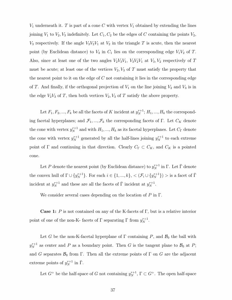
V1 underneath it. T is part of a cone C with vertex V1 obtained by extending the lines

joining V1 to V2, V3 indefinitely. Let C1, C2 be the edges of C containing the points V2,

V3 respectively. If the angle V3V2V1 at V2 in the triangle T is acute, then the nearest

point (by Euclidean distance) to V3 in C1 lies on the corresponding edge V1V2 of T .

Also, since at least one of the two angles V2V3V1, V3V2V1 at V3, V2 respectively of T

must be acute; at least one of the vertices V2, V3 of T must satisfy the property that

the nearest point to it on the edge of C not containing it lies in the corresponding edge

of T . And finally, if the orthogonal projection of V1 on the line joining V2 and V3 is in

the edge V2V3 of T , then both vertices V2, V3 of T satisfy the above property.

Let F1, F2, ..., Fk be all the facets of K incident at yr+1N ; H1, ..., Hk the correspond-

ing facetal hyperplanes; and F1, ...,Fk the corresponding facets of Γ. Let CK denotethe cone with vertex yr+1N and with H1, ...,Hk as its facetal hyperplanes. Let CΓ denote

the cone with vertex yr+1N generated by all the half-lines joining yr+1N to each extreme

point of Γ and continuing in that direction. Clearly CΓ ⊂ CK , and CK is a pointed

cone.

Let P denote the nearest point (by Euclidean distance) to yr+1N in Γ. Let Γ denote

the convex hull of Γ ∪ yr+1N . For each i ∈ 1, ..., k, < (Fi ∪ yr+1N ) > is a facet of Γincident at yr+1N and these are all the facets of Γ incident at yr+1N .

We consider several cases depending on the location of P in Γ.

Case 1: P is not contained on any of the K-facets of Γ, but is a relative interior

point of one of the non-K- facets of Γ separating Γ from yr+1N .

Let G be the non-K-facetal hyperplane of Γ containing P , and B0 the ball withyr+1N as center and P as a boundary point. Then G is the tangent plane to B0 at P ;and G separates B0 from Γ. Then all the extreme points of Γ on G are the adjacent

extreme points of yr+1N in Γ.

Let G+ be the half-space of G not containing yr+1N , Γ ⊂ G+. The open half-space

37

of G containing yr+1N , G− = Rn\G+ satisfies Γ\Γ ⊂ G−, and also Γ\Γ ⊂ K\Γ.

Let y1N be an extreme point of Γ on G that is the nearest to yr+1N among all

the extreme points of G. Let H be the hyperplane through P orthogonal to the line

segment y1NP and G; so H contains yr+1N . Let H+, H− be the half-spaces defined by

H, containing y1N , not containing y1N respectively.

Let H1 be a facetal hyperplane of K incident at yr+1N that contains y1N . Let B1be the ball with yr+1N as center and y1N as a boundary point. B1, B0 are concentricspheres with B0 contained inside B1. The half-space H+

1 of H1 containing K contains

the half-balls B+0 , B+1 of B0, B1 respectively on the side of H1 containing K. LetB++1 = B+1 ∩H+, B+−1 = B+1 ∩H−.

For any point yN ∈ Γ∩G∩H−, it can be verified that the hyperplane T throughyN orthogonal to the line segment y

1NyN has both the points y

1N , y

r+1N on the same side;

which implies that the angle y1NyNyr+1N at yN in the triangle y

1Ny

Nyr+1N is strictly acute.

This in turn implies, by the 2-dimensional results mentioned at the beginning of

this proof, that the nearest point to y1N on the half-line joining yr+1N to yN and continuing

in that direction, is on the line segment joining yr+1N and yN but not including the point

yN , so it is in Γ\Γ ⊂ K\Γ.

We will now consider two subcases.

Case 1.1: Suppose for some i ∈ 1, ..., k, Fi not containing y1N satisfies Fi∩G ⊂H−.

Let x+1i denote the nearest point in Fi to y1N , and let U denote the half-line

joining yr+1N to x+1i and continuing in that direction. By the definition of x+1i , it must

be the nearest point to y1N on U ∩ Γ.

Since x+1i ∈ Fi, and Fi ⊂ G+, we know that x+1i ∈ G+. So, U must intersect G.

Suppose U intersects G at x−1i . Clearly, x−1i ∈ Γ ∩ G ∩ H−, and the half-open

line segment U− joining yr+1N to x−1i but not including x−1i is a subset of K\Γ.

38

Then from the above facts we know that nearest point by Euclidean distance to

y1N on U is in U−, which implies that the nearest point to y1N in Fi is in Fi\Fi.

This shows that in this subcase, the final step carried out with the known extreme

point y1N and facet Fi of K will show that at this stage Fi = Fi and lead to a new

extreme point in Fi\Fi to add to the present list of extreme points.

Case 1.2: For all i ∈ 1, ..., k such that Fi does not not contain y1N satisfies

Fi ∩G is not a subset of H−.

So in this case, for all i ∈ 1, ..., k such that y1N ∈ Fi, H+ contains a relative

interior point of G∩Fi, which in turn implies that at least one extreme point of G∩Fiis in the interior of H+.

Now extend the line joining y1N to P until it intersects the boundary of G ∩ Γagain; suppose it intersects it at a point yN . Since the line segment joining y

1N and yN

contains a relative interior point P of G, facets of Γ containing yN do not contain y1N

and vice versa. We will now consider two subcases.

Case 1.2.1: yN is itself an extreme point of Γ.

In this case the hyperplane through P orthogonal to the line segment yNP is the

hyperplane H itself discussed at the beginning of Case 1, but in this case what we

called H+ in Case 1 is the half-space of H not containing yN .

In this case all the facets Fi for i ∈ 1, ..., k, G of Γ incident at yN have a

relative interior point intersection with H+, i.e., at least one extreme point on it is in

the interior of H+. Since K belongs to Class 2, this implies that there must be at least

one j ∈ 1, ..., k such that Fj∩G ⊂ G∩H+. In fact some Fj for j ∈ 1, ..., k incidentat y1N satisfies this property also. So, from the hypothesis of this case we conclude that

this Fj does not contain yN .

Using this fact and arguments similar to those in Case 1 with yN replacing y1N , we

39

conclude that for all points yN ∈ Γ∩G∩H+, the hyperplane T through yN orthogonal to

the line segment yNyN has both the points yN , yr+1N on the same side, which implies that

the angle yNyNyr+1N at yN in the triangle yNyNy

r+1N is strictly acute, and consequently

the nearest point to yN in the half line joining yr+1N to yN and cotinuing in that direction,

is in the intersection of this half-line with Γ\Γ ⊂ K\Γ. Continuing as in Case 1.1, weconclude that the nearest point to yN in Fj is different from that in Fj, and thereforethat the final step carried out with the extreme point yN and the facet Fj of K will

generate a new extreme point of K not in Γ.

Case 1.2.2: yN is not an extreme point of Γ.

Let S denote the smallest dimensional face of Γ∩G containing yN . Then yN is arelative interior point of S, and it can be expressed as a convex combination of extreme

points of S.

S is the intersection of G and all the Fi for i ∈ 1, ..., k that contain it as asubset. Let SI = i : i ∈ 1, ..., k and S is a subset of Fi. Since y1N , yN are not bothcontained together on any Fi for i ∈ 1, ..., k, we know that y1N ∈ Fi for all i ∈ SI .Also, from the hypothesis we know that for all i ∈ SI , Fi has a relative interior pointintersection with the half-space H+.

Let y2N be an extreme point of S. Let H2 be a facetal hyperplane of K incident

at yr+1N containing y2N . As y2N ∈ B+1 ∩H−, H2 passes through B+−1 defined earlier. Let

H+2 be the half-space of H2 containing K. Then K ⊂ H+

2 ∩H+1 .

Let H2 be the hyperplane through P orthogonal to the line segment y2NP , and H2

also contains the line segment Pyr+1N . So H2 is obtained by tilting H discussed earlier

on the line segment Pyr+1N while keeping its orthogonality with G.

Let H+2 , H

−2 denote the half-spaces of H2 containing y

2N , not containing it, re-

spectively.

From the arguments under Case 1.2.1, we already know that in this case there

exists a facet Fj of Γ incident at yr+1N and containing the point y1N , and satisfying

40

Fj ∩G ⊂ G∩H+. So, we can select an extreme point y2N on S such that H2 obtained

by tilting H on the line Pyr+1N satisfies the property that H−2 contains this Fj ∩G.

Repeating the arguments made under Case 1 with respect to y1N , but now with

the point y2N , we conclude that for all yN ∈ Fj ∩ G, the angle y2NyNyr+1N at yN in the

triangle y2NyNyr+1N , is strictly acute.

So, continuing with arguments similar to those made earlier, we conclude that

the final step carried out with this extreme point y2N and the facet Fj of K will find a

new extreme point on Fj to add to Γ.

Case 2: P is contained on a K-facet Fv say, of Γ.

Since Γ ⊂ CΓ discussed earlier, clearly v ∈ 1, ..., k, and so P ∈ Fv and thehalf-open line segment [yr+1N P ) joining yr+1N to P but not containing P is a subset of

Fv\Fv.

Again let B0 be the ball with yr+1N as center and P as a boundary point. Let L

be the tangent plane to B0 at P in this case, so L is orthogonal to Hv; and denote thehalf-space of Hv containing K by H+

v . Let L+ denote the open half-space of L on the

side of Γ; and L− the other closed half-space of L that contains yr+1N . Also L+ ∪ L =L+, the closure of L+.

If all the extreme points of Fv are in the open half-space L+, then Fv, theirconvex hull will itself be contained in this open half-space, contradicting that P ∈ Fv.So, L ∩ Fv must have at least one extreme point of Fv.

We will now consider several subcases.

Case 2.1: P contained in the relative interior of Fv, in the relative interior of an

(n− 2)-dimensional face of Fv.

P must be contained in the (n − 2)-dimensional intersection of Fv with somenon-K-facet of Γ, let that non-K-facet of Γ be denoted by G. These facts imply that

G∩Fv = L∩Fv = S say. All the extreme points of this (n− 2)-dimensional face S of

41

Γ are in L and in G.

Let y1N be an extreme point of Γ in L ∩ Fv and H be the hyperplane through P

orthogonal to the line segment y1NP , so H is orthogonal to L and Hv, and contains the

line segment Pyr+1N .

Let H+ the half-space of H containing y1N ; and H− the other half-space of H. It

can be verified that for any point yN ∈ L∩H−, the angle y1NyNyr+1N at yN in the triangle

y1NyNyr+1N is acute. So, for some i ∈ 1, ..., k such that y1N ∈ Fi, if Fi ∩ L ⊂ H−, then

this fact together with all the arguments used earlier leads to the conclusion that the

nearest point to y1N on the line joining yr+1N to yN and continuing in that direction, for

any yN ∈ Fi ∩ L is on the side of L containing yr+1N .

Also, in this case for any i ∈ 1, ..., k such that Fi does not contain y1N , and anypoint y N ∈ Fi∩G, the line segment yr+1N yN must intersect L at some point yN ∈ L∩Fi.

Using all these arguments together we conclude that the nearest point to y1N in

Fi for that i, is different from the nearest point to it in Fi; again showing that in thiscase the final step will generate a new extreme point of K not in Γ.

If all the Fi not containing y1N for i ∈ 1, ..., k have a relative interior point

intersection with H+, then extend the line joining y1N to P until it intersects the

relative boundary of Fv again. Suppose this point of intersection is yN .

If yN is an extreme point of Fv, using arguments similar to those in Case 1.2.1,we can again show that the final step carried out with yN and a facet Fi containing y

1N

for some i ∈ 1, ..., k will generate a new extreme point of K not in Γ.

If yN is not an extreme point of Fv, we can use arguments similar to those inCase 1.2.2, and again conclude that the final step will generate a new extreme point of

K not in Γ.

Case 2.2: P is itself an extreme point of Fv

Here let H be the hyperplane through P containing the line segment Pyr+1N , and

42

orthogonal to Hv, and L.

In this case, there must be at least one facet Fi for i ∈ 1, ..., k not containingP such that Fi is on one side of H. Since the line Pyr+1N is orthogonal to L, it can

be verified that the angle PyNyr+1N at yN in the triangle PyNy

r+1N is strictly acute for

any yN ∈ L ∩Fi for such an i. Using this and arguments similar to those in Case 2.1,we again conclude that the final step applied with P and the facet Fi for that i will

generate a new extreme point of K not in Γ in this case also.

Case 2.3: P is in the relative interior of a face S of Fv of dimension between 2and n− 3.

So in this case S ⊂ L ∩Fv.

S must be the intersection of some non-K-facet of Γ, let G be one of those.

Let y1N be an extreme point of S. Here we argue similar to that in Case 2.1

with S taking the role of Fv. H,H+,H− are defined as in Case 2.1. If all the Fi for

i ∈ 1, ..., k not containing y1N have a relative interior point intersection with H+,

then we extend the line joining y1N to P until it intersects the relative boundary of

S again, call this point of intersection as yN ; then continue the arguments similar to

those in Case 2.1 and 1.2.2. Again, we can conclude that the final step will generate a

new extreme point of K not in Γ in this case also.

Hence if the final step does not output a new extreme point of K not in Γ, then

Γ = K, when K belongs to Class 2 defined in Section 8.

If the mukkadvayam Γ = K, these results show that the final step of Section 9

will generate a new extreme point of K to add to Γ, and continue the enumeration if

K belongs to Class 2 defined in Section 8. Clearly the number of linear programs and

convex quadratic programs to be solved in all these steps is bounded above by O(r3)

and O(r(n + m)) respectively. So the procedure consisting of all the steps discussed

above provides a polynomial time algorithm for extreme point enumeration when K

43

belongs to Class 2.

Even when K belongs to Class 1 defined in Section 8, I believe that the whole

procedure including the mekkadvayam checking step of Section 8 will enumerate all

the extreme points of K, but do not have a proof of it yet.

Acknowledgements: Discussions with Santosh Kabadi of The University of

New Brunswick at Frederiton, NB, Canada, and with my colleague Romesh Saigal have

been very helpful, for which I am very grateful. Also, Hans Raj Tiwary [11] constructed

a 5-dimensional counterexample to an earlier version of the algorithm not including the

final step which has been very helpful, I am grateful to him. My thanks to the referees,

and their many detailed suggestions to improve the content and writeup in the paper.

Some of this work was done while visiting the GSLM Department of NDHU (National

Dong Hwa University) in Hualien, Taiwan, at the invitation of its Director Yat-wah

Wan in 2007, 2008. I thank him and his Colleagues for the stimulating environment in

their Department, and for inviting me.

11 References

[1] A. Y. Alfakih, T. Yi, K. G. Murty, “Facets of an Assignment Problem with a 0− 1Side Constraint”, Journal of Combinatorial Optimization, 4(2000)365-388.

[2] D. Avis and K. Fukuda, “A pivoting algorithm for convex hulls and vertex enumera-

tion of arrangements and polyhedra”, Discrete and Computational Geometry 8(1992)295-

313.

[3] G. B. Dantzig, Linear Programming and Extensions, Princeton University Press,

1963.

[4] B. Grunbaum, Covex Polytopes, Wiley Interscience, NY, 1967.

[5] L. Khachiyan, E. Boros, K. Borys, K. Elbassioni, and V. Gurvich, “Generating All

Vertices of a polyhedron is Hard”, RUTCOR, Rutgers university, 2006.

[6] K.G. Murty, “Adjacency on convex polyhedra”, SIAM Review 13, no. 3(1971)377-

44

386.

[7] K.G. Murty, Linear Programming (Wiley, NY, 1983).

[8] K.G. Murty, S. J. Chung, “Segments in Enumerating Facets”, Mathematical Pro-

gramming 70(1995)27-45.

[9] K. G. Murty, “A New Practically Efficient Interior Point Method for LP”, Algorith-

mic Operations Research, 1(2006)3-18.

[10] J.S. Provan, “Efficient enumeration of the vertices of polyhedra associated with

network LPs”, Mathematical Programming 63(1994)47-64.

[11] H. R. Tiwary, Private communication, 2007.

[12] G. M. Ziegler, Lectures on Polytopes, Springer-Verlag, NY, 1994.

45