Ple

ase

note

that

this

is a

n au

thor

-pro

duce

d P

DF

of a

n ar

ticle

acc

epte

d fo

r pub

licat

ion

follo

win

g pe

er re

view

. The

def

initi

ve p

ublis

her-a

uthe

ntic

ated

ver

sion

is a

vaila

ble

on th

e pu

blis

her W

eb s

ite

1

Ecological Modelling Vol. 193, Issues 3-4 , 15 March 2006, Pages 295-314 http://dx.doi.org/10.1016/j.ecolmodel.2005.08.036 © 2005 Elsevier B.V. All rights reserved

Archimer, archive institutionnelle de l’Ifremerhttp://www.ifremer.fr/docelec/

A probabilistic approach of flow-balanced network

based on Markov chains

Delphine Leguerriera, b, Cédric Bacherc,*, Eric Benoîtd and Nathalie Niquila aLaboratoire de Biologie et Environnement Marins, FRE 2727 CNRS, Université de La Rochelle, Pôle Sciences et Technologie, Avenue Michel Crépeau, 17042 La Rochelle Cedex 1, France bCentre de Recherche sur les Ecosystèmes Marins et Aquacoles (CREMA/UMR10 CNRS-IFREMER), BP 5, 17137 L’Houmeau, France cIFREMER, B.P. 70, 29280 Plouzané, France dLaboratoire de Mathématiques, Université de La Rochelle, Pôle Sciences et Technologie, Avenue Michel Crépeau, 17042 La Rochelle Cedex 1, France *: Corresponding author : cbacher@ifremer.fr

Abstract: We used Markov chains to assess residence time, first passage time, rate of transfers between compartments, recycling index with a general mathematical formalism. Such a description applies to any flow-balanced system that can be modelled as a series of discrete stages or compartments through which matter flows. We derived a general set of equations from a probabilistic approach and applied them to a food web and a physical system derived from the literature. We therefore analysed preferential pathways of matter and behaviour of these systems and showed how it was possible to build up and exploit indices on the basis of a transition probability matrix describing the network, and to characterize with a generic algorithm: (1) the total indirect relationships between two compartments, (2) the residence time of one compartment and (3) the general recycling pathways including the amount of matter recycling and the implication of each compartment in recycling. Keywords: Markov chain; Residence time; Transfer rate; Network; Food web model; Box model; First passage time

A probabilistic approach of flow-balanced network based on

Markov chains Delphine Leguerrier1-2, Cédric Bacher3, Eric Benoît4, Nathalie Niquil1 1 Laboratoire de Biologie et Environnement Marins, FRE 2727 CNRS, Université de La

Rochelle, Pôle Sciences et Technologie, avenue Michel Crépeau, 17042 La Rochelle

Cedex 1, France 2 Centre de Recherche sur les Ecosystèmes Marins et Aquacoles (CREMA/UMR10

CNRS-IFREMER), BP 5, 17137 L’Houmeau, France 3 IFREMER, BP 70, 29280 Plouzané, France 4 Laboratoire de Mathématiques, Université de La Rochelle, Pôle Sciences et 10

Technologie, avenue Michel Crépeau, 17042 La Rochelle Cedex 1, France

Corresponding author: C. Bacher, cbacher@ifremer.fr

Key words: Markov chain, residence time, transfer rate, network, food-web model, box

model, first passage time

Abstract

We used Markov chains to assess residence time, first passage time, rate of transfers between

compartments, recycling index with a general mathematical formalism. Such a description

applies to any flow-balanced system that can be modelled as a series of discrete stages or 20

compartments through which matter flows. We derived a general set of equations from a

probabilistic approach and applied them to a food web and a physical system derived from

the literature. We therefore analysed preferential pathways of matter and behaviour of these

systems and showed how it was possible to build up and exploit indices on the basis of a

transition probability matrix describing the network, and to characterize with a generic

algorithm: (1) the total indirect relationships between two compartments, (2) the residence

time of one compartment and (3) the general recycling pathways including the amount of

matter recycling and the implication of each compartment in recycling.

Introduction

Ecosystem behaviour is driven by different temporal and spatial scales of biological and 30 physical processes. Because of the spatial boundaries of a system, any matter (salt or fresh water, carbon, nitrogen or any substance) flowing through it will remain for a period which

* Manuscript

depends on the interactions between the process involved and the type of matter. Therefore, assessing matter cycling, pathways and residence time within ecosystem compartments can help in understanding ecosystem properties. For deterministic systems based on interactions between compartments - whether this be matter transfer as described by Guangso et al. 2002, Thompson et al. 2002, Sivakumar et al. 2005, Yu & Wehrby 2004, or changes of the system from one state to another as described by Logofet & Lesnaya 2000 - probability of transition from one compartment to another can be defined during a given time. Assuming that transition probabilities are time-independent, this corresponds to a Markov-chain model, 40 where the state of the system at time s > t can be predicted from the knowledge of the state of the system at time t and does not depend on the situation before t (Markov property, Bailey 1964). Markov-chain models are particularly adapted to the study of succession processes such as forest successions (Logofet & Lesnaya 2000, Benabdellah et al. 2003), metapopulation dynamics (Moilanen 2004), or the evaluation of transit times of tracers in various environments. Examples of transit though environments include: transit in a gasifer (Guangso et al. 2002), of a particle in a tidal mixing estuary (Thompson et al. 2002), of a solute in an aquifer system (Sivakumar et al. 2005) and of drugs within the body (Yu & Wehrby 2004). Description of this type also applies to ecological studies. Odum (1959) defined ecology as 50 “the study of the relationships of organisms with one another and with their non-living environment” and the magnitude of matter and energy flows between the various components of an ecosystem is now regarded as an appropriate measure of such relationships (Szyrmer & Ulanowicz, 1987). A food web is therefore a good method for the quantitative description of an ecosystem (Ulanowicz 1984). The food web can be seen as a graph, with nodes (the compartments) and quantitative links (the trophic fluxes between them). Such a representation might seem static and non-evolutive, as would a still photograph of the ecosystem. Yet trophic dynamic aspects emerge from such representations (Lindeman 1942). Once the food web is drawn, this often complex scheme can be transformed into a more synthetic representation which reveals the emergent properties of the system (Ulanowicz 1986). When 60 studying the interrelations between components of a food web, looking at direct interactions (first passage flows) is not enough and one has also to consider subsequent passage flow from a holistic point of view (Patten, 1995). Hannon (1973) applied Leontief’s Input-Output analysis (Leontief, 1936, 1951) to ecology, in order to study the interdependence of organisms in an ecosystem. The central element in this theory is the Leontief structure matrix, which is commonly thought to express the total direct and indirect flows between any two compartments of a system (Szyrmer & Ulanowicz, 1987). Two parallel conceptions can be distinguished in input-output analysis. These are Leontief’s backward formalism, which from the outputs of the systems deduces the necessary inputs, and Augustinovicz’s forward formalism, which calculates the fate of outputs from the compartments, thus deducing the 70

transit of the matter from the inputs to the system (Kay et al. 1989). The direct interactions are shown by the two-dimensional matrix of internal exchanges, and much information can be obtained about the indirect links through straightforward operations on the matrix of direct flows (Ulanowicz, 1984). The multiplicity of possible pathways within the food web are translated into indices based on thermodynamics and information theory, such as Ascendency, Redundancy and Overheads (Ulanowicz 1986, Ulanowicz & Norden 1990). By introducing the idea of temporality into this conception, Higashi et al. (1993) gave importance to the biomass of the compartments. In their description, the transfer of matter (energy, carbon, biomass etc.) from one compartment to another can be delayed by storage in the compartments. Hence, each flow is a possible pathway for matter which is taken with a 80 certain probability. This describes a Markov process in which matter is transferred or retained in the food web at each time-step, depending only on its previous trajectories. Markov transition probability matrices can be constructed according to the two conceptions of information theory, backward or forward cases (Kay et al. 1989). Residence time has received a lot of attention as a useful indicator in physical oceanography. Several definitions of residence time can be found in the literature. According to Takeoka (1984a), transit time should be distinguished from residence time. The first deals with the time water particles take to cross an area from entrance to exit. For the second, all the particles contained in the area are considered. In this case, the residence time corresponds to the mean transit time but depends on the initial location of the particles. Takeoka (1984a) 90 showed that the difference between the two mean temporal characteristics could be defined as the age of the particles retained in the area. In a general approach, Bolin and Rodhe (1972) summarized and compared the basic concepts of age distribution and transit time showing that the mean transit time equals the so-called ‘turnover time’ (defined as the ratio between the volume and the total inflow). Following Zimmerman (1976), Takeoka (1984b) compared residence and transit time scales. He solved the case of a one-dimensional channel with uniform advection and longitudinal diffusion. Zimmerman (1976) used salinity distribution and a box model to assess the exchange terms between the boxes and the spreading of a tracer in the Wadden Sea, under the assumption of a steady-state. Numerical integration of the transport equation yielded residence time estimations in each spatial box. Dronkers and 100 Zimmerman (1982) derived an estimation of the residence time and the age of fresh water in the Oosterschelde from a steady state unidimensional and dispersive equation. Once again the dispersion coefficients were estimated from salinity distribution. Using a box model and a salt balance equation, Miller and McPherson (1991) computed the residence time in an one-dimensional case through the simulation of the salt transport with different initial conditions corresponding to the initial vector filled with values 0 or 1 in some boxes. Recently, Thompson et al. (2002) used a Markov chain approach combined with a spatial box model to characterise water mixing and transport within a bay.

In our study, we develop Markov chains further to construct a series of indicators: residence time, first passage time, rates of transfer between compartments and number of passages in a 110 compartment. Since such a description applies to any flow-balanced system that can be modelled as a series of discrete stages or compartments through which matter flows, we applied Markov chains to a food web (Takapoto atoll food web, Niquil et al. 2001) and a physical system (Passamaquoddy Bay tidal mixing model, Thompson et al. 2002). We used our indicators to analyse preferential pathways of matter and behaviour of these systems.

Methods

Markov transition matrix

Food-web matrix F

The food-web matrix F describes all the flows between N compartments and between

compartments and the exterior of the system. Flows are given in matter (energy, carbon, 120

biomass …) per unit of time (day, year). The formalism is derived from Finn (1976), Patten &

Higashi (1995) and Fath & Patten (1998): elements Fij define the flow going from

compartment j to compartment i. The last column and row give respectively the inputs from

the exterior of the system, and the outputs from the compartments. The internal flow matrix

concerns only the exchanges between compartments of the system. The food web is

described at steady state, which means that the total output from any compartment (Touti -

sum of corresponding column) equals the total input to this compartment (Tini - sum of the

corresponding row). Each compartment has a known biomass Bi.

Transition matrix P

According to the Higashi et al (1993) view of flow temporality, the probability that a particle 130

which is in compartment j (j = 1..N) at time t passes to compartment i (i = 1..N+1) during one

time step ∆t is equal to:

( )/ ijij

j

FP j i j P tB→ = = ⋅ ∆

Probability for a particle that is in i to stay in i during one time step is given by:

( ) 1,/ 1ii ki N ik i

P i i j P P P +≠

→ = = − −∑

Time step ∆t must be chosen so that each term of matrix P is positive and less than 1. Any

choice for this time step will lead to the same results, provided that it is small enough to

represent less that the time needed to empty any compartment (the minimum of turnover

times defined as the biomass of a compartment divided by the sum of all its exiting flows).

Hence, we chose half the minimum of turnover times computed for all compartments. From 140

here on, time will be expressed as a number of time steps. The matrix P is completed by

adding a column for the exterior of the system: a column of zeros, with 1 for the last element

which is an absorbing element. This matrix is column-stochastic since the sum of each of its

column is one (Bailey 1964). It is the transition matrix of a Markov process, in which the

random variable is the concentration C of a tracer in each compartment. Given the initial state 0C of a particle in the system and 0

iC the probability that the particle is in compartment i at

time 0, the concentration at time t+∆t is equal to: 1t tC P C+ = ⋅

hence 0t tC P C= ⋅ (1) 150

Distribution Ct+1 only depends on state Ct and not on the previous states, which is the

characteristic of the Markov property (Bailey 1964). In the following descriptions, C will

always be less than 1, and hence represents the probability distribution of a unit of matter

within the food web. As time is incremented, one can then compute the probability

distribution of a unit of matter, or, as Thompson et al. (2002), compute the probability that a

particle stays in a compartment in which it was at time t = 0, the probability that a particle is

absorbed by the exterior compartment, or the probability that a particle moves from one

compartment to another for the first time during time t. With the latest representation, another

computation is necessary. For each compartment i we constructed a new matrix Qi in which i

is an absorbing compartment: the ith column is replaced by a column of zeros, with 1 at the ith 160

position. Qi is also a Markov transition matrix, and we can also compute (see Results): 0t t

iC Q C= ⋅

Calculation of indices from a Markov transition probability matrix

In the following we will use the Markov transition probability matrix P and generator

functions to compute analytically the average passage time and the transfer rate from

compartment j to compartment i.

Transfer rate and transit time

Let us define ,i tA as the event of being in compartment i at time 0t ≥ , ,i tC as the event of being

in compartment i for the first time at time t>0 and , ,i j tC as the subset of ,i tC corresponding to

being in j at time 0. We write the conditional probability , ,i j tc as , , , ,0( / )i j t i t jc P C A= . We 170

define the average passage time Tij as the expectation of the random variable t associated with

the probability distribution , ,i j tc , and the transfer rate Rij as the average of the probability

distribution , ,i j tC . Using the generator functions ( ), , ,0

ki j i j k

ks c sγ

∞

=

= ⋅∑ and

( ), , ,0

ki j i j k

ks a sα

∞

== ⋅∑ , we can write:

( ), 1i jij

dT s

dsγ

= = (2)

and

( ), 1ij i jR γ=

The conditional probability , , , ,0( / )i j t i t ja P A A= is easily derived from the transition matrix P

using equation (1) and it is easy to show that:

( ) ( ) 1, ,i j i j

s s Pα −= Ι − ⋅ 180

where I is the identity matrix. In the following, we will show how to derive ( ),i j sγ from

( ),i j sα .

When one lists all the elements of , ,i j tC , all the events where i has been reached at least once

before time t must be excluded. The product , , , ,i j t k i i ka c− ⋅ gives the probability of being in i at

time t-k and coming again to compartment i after exactly k steps. Therefore we can write: 1

, , , , , , , ,1

t

i j t i j t i j t k i i kk

c a a c−

−=

= − ⋅∑

We will see below that it is necessary to extend the summation from k = 0 up to t. We

introduce the new element , ,0i ic , which can be arbitrarily chosen, and write:

, , , , , , , , , , , ,0 , ,0 , ,0

t

i j t i j t i j t k i i k i j t i i i j i i tk

c a a c a c a c−=

= − ⋅ + ⋅ + ⋅∑

If i≠j, , ,0 0i ja = and the equation becomes: 190

, , , , , , , , , , , ,00

t

i j t i j t i j t k i i k i j t i ik

c a a c a c−=

= − ⋅ + ⋅∑ (3)

and is valid for t>0. To extend the above equation to the case t = 0, we must define a new

term , ,0 0i jc = and it is valid for all t.

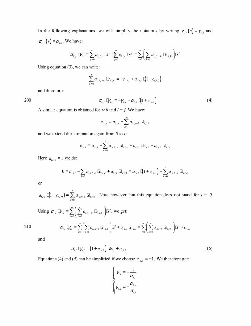
In the following explanations, we will simplify the notations by writing ( ), ,i j i jsγ γ= and

( ), ,i j i jsα α= . We have:

, , , , , , , , , ,0 0 0 0

tp q t

i j i i i j p i i q i j t k i i kp q t k

a s c s a c sα γ∞ ∞ ∞

−= = = =

⋅ = ⋅ ⋅ ⋅ = ⋅ ⋅

∑ ∑ ∑ ∑

Using equation (3), we can write:

( ), , , , , , , , , ,00

1t

i j t k i i k i j t i j t i ik

a c c a c−=

⋅ = − + ⋅ +∑

and therefore:

( ), , , , , ,01i j i i i j i j i icα γ γ α⋅ = − + ⋅ + (4) 200

A similar equation is obtained for t>0 and I = j. We have: 1

, , , , , , , ,1

t

i i t i i t i i t k i i kk

c a a c−

−=

= − ⋅∑

and we extend the summation again from 0 to t:

, , , , , , , , , , , ,0 , ,0 , ,0

t

i i t i i t i i t k i i k i i t i i i i i i tk

c a a c a c a c−=

= − ⋅ + ⋅ + ⋅∑

Here , ,0 1i ia = yields:

( ), , , , , , , , , ,0 , , , ,0 , , , ,0 0

0 1t t

i i t i i t k i i k i i t i i i i t i i i i t k i i kk k

a a c a c a c a c− −= =

= − ⋅ + ⋅ = ⋅ + − ⋅∑ ∑

or

( ), , , ,0 , , , ,0

1t

i i t i i i i t k i i kk

a c a c−=

⋅ + = ⋅∑ . Note however that this equation does not stand for t = 0.

Using , , , , , ,0 0

tt

i i i i i i t k i i kt k

a c sα γ∞

−= =

⋅ = ⋅ ⋅

∑ ∑ , we get:

, , , , , , , ,0 , ,0 , , , , , ,01 0 1 0

t tt t

i i i i i i t k i i k i i i i i i t k i i k i it k t k

a c s a c a c s cα γ∞ ∞

− −= = = =

⋅ = ⋅ ⋅ + ⋅ = ⋅ ⋅ +

∑ ∑ ∑ ∑ 210

and

( ), , , ,0 , , ,01i i i i i i i i i ic cα γ α⋅ = + ⋅ + (5)

Equations (4) and (5) can be simplified if we choose , ,0 1i ic = − . We therefore get:

,,

,,

,

1i i

i i

i ji j

i i

γαα

γα

= − = −

The average passage time Tij is the first order derivate of the generator function γi,j(s) for s = 1

(equation (2)). It may be proved (not shown) that this derivative always exists even in cases

where γi,j(1) is not finite. It was computed as the limit:

( ) ( ), ,0

1 2 1lim i j i j

ijT ε

γ ε γ εε→

− ⋅ − −=

and the transfer rate Rij as the value:

( ), 1ij i jR γ= 220

Adaptation to various issues

Conditional probabilities

The Tij and Rij (i = 1..N, j = 1..N, N+1 being the exterior compartment) coefficients computed

from the paragraph above represent the time taken to reach the compartment i and the amount

of matter that will reach the compartment i, when one unit of matter is in compartment j at t =

0. In this calculation we can split the matter into two categories, matter which leaves j within

the first time step and matter which stays longer in j. When we want to calculate transit time

and transfer rate for the first category of matter therefore, we consider the fate of matter

depending on whether it leaves compartment j at time 0.

We define two sets of conditional probabilities. 'kjP is the probability that a particle living j 230

arrives to compartment k within one time step (k = 1..N+1, k ≠ j), and "kjP is the probability

that a particle leaving j arrives to compartment k with the additional condition that the particle

stays within the system (k = 1..N, k ≠ j).

A planktonic theoretical food web provides a small theoretical example for an explanation.

The example food web has 4 compartments: ‘phytoplankton’ (“phyto”, compartment n°1),

‘bacteria’ (“bact”, n°2), ‘zooplankton’ (“zoo”, n°3), and ‘detritus’ (“det”, n°4) (Figure 1).

Assuming that the transition probability matrix P has been defined on the basis of the food-

web matrix and considering the case of bacteria compartment (n°2), we defined conditional

probabilities as following:

' 1212

12 32 42 2

' 3232

12 32 42 2

' 4242

12 32 42 2

ext

ext

ext

PP

P P P PP

PP P P P

PP

P P P P

= + + +

= + + +

=+ + +

and

" 1212

12 32 42

" 3232

12 32 42

" 4242

12 32 42

PP

P P PP

PP P P

PP

P P P

= + +

= + +

=+ +

240

Conditional transfer rates

Transfer rate is defined as the fraction of matter leaving compartment j that will reach the

compartment i. Supposing that a particle has left the compartment j between time t = 0 and ∆t

(during the first step). P’ represents the probability that the particle either reached another

compartment or left the system. Then, at each time step, matter can exit the system, be

transferred to another compartment, or stay where it is. The conditional transfer rates ijRC

from the bacterial compartment (j = 2) to other compartments i ≠ j were derived from ijR as

following: ' ' '

42 41 12 43 32 421RC R P R P P= ⋅ + ⋅ + ⋅

For i = j = 2, we write: 250 ' ' '

22 21 12 23 32 24 42RC R P R P R P= ⋅ + ⋅ + ⋅

Conditional transit times

Conditional transit time TCij is the time taken by a particle that leaves compartment j between

t = 0 and t = ∆t to reach the target compartment i. Two cases must be distinguished: the transit

time from one compartment to another is computed using P’’ probability, and the transit time

from one compartment to outside (residence time of the compartment) is not changed,

because it represents the residence time of one compartment, i.e. the time taken to get out of

the system assuming that the matter is in the compartment at time t = 0. As above conditional

transit times ijTC were derived from ijT for i = 4 and j = 2 as following:

" " "42 41 12 43 32 421TC T P T P P= ⋅ + ⋅ + ⋅ 260

For i = j=2 we write: " " "

22 21 12 23 32 24 42TC T P T P T P= ⋅ + ⋅ + ⋅

Return time and number of passages

Rii defines the return rate to compartment i and corresponds to the fraction of biomass that

comes back for the first time to compartment i. The average number of passages Nii can easily

be derived from the successive fractions iiR , 2iiR , 3

iiR , …, kiiR , …We write:

1

kii ii

kN R k

∞

== ⋅∑

Since 1

1 1 0

k k kii ii ii ii ii

k k kii

dR k R R k R R

dR

∞ ∞ ∞−

= = =

⋅ = ⋅ ⋅ = ⋅

∑ ∑ ∑ and 0

11

kii

k ii

RR

∞

==

−∑ , we get:

( )21ii

iiii

RNR

=−

Applications 270

The first application was made to Takapoto lagoon (TA) pelagic food-web model analysed

by Niquil et al. (2001) who aggregated organic carbon stocks into eight living and two non-

living compartments (Table 1), which structure the ecosystem on the basis of processes and

sizes (Figure 2a). The compartments were: bacteria (BAC), phytoplankton < 1 µm (PH1),

phytoplankton from 1 to 3 µm (PH2), phytoplankton > 3 µm (PH3), protozoa < 35 µm (PZ1),

protozoa > 35 µm (PZ2), microzooplankton < 250 µm (MIC) and mesozooplankton from 250

to 2000 µm (MES), dissolved organic carbon (DOC) and particulate organic carbon (POC).

Flows between planktonic compartments (Table 2a) were partly determined by field

experiments and completed by inverse analysis (Vézina & Platt 1988). The second application

concerns Passamaquoddy Bay (PB) box model developed by Thompson et al. (2002) who 280

characterised water mixing with a discrete-time, finite-state Markov Chain model. The bay

was divided into 15 homogeneous regions ('boxes') (Figure 2b) and transition probabilities

were estimated by computing a lot of trajectories by the means of two-dimensional

hydrodynamic model (Table 3). Initially the time unit was the tidal cycle (one flow and one

ebb). In the following we have used day units by considering that 2 tidal cycles occurred

during one day.

From here on, T and R will refer to the final computed transit time and transfer rate (after use

of conditional probabilities).

Results and discussion

Tracking a particle within the ecological network 290

P matrix structure

The elements of the P matrices generally correspond to direct links between compartments of

the systems. However, some unusual values should be mentioned. In the PB model, some

probabilities existed between zones that are not physically linked (which can be seen on the

map, Figure 2b, in Thompson et al. 2002), due to the fact that transition probabilities are

based on simulations (with a hydrodynamical model) of particle trajectories which may cross

several spatial compartments within one day. Therefore the probability that a particle exiting

the system from compartment 7 or 8, for example, is not zero even though 7 and 8 are not

physically linked to the boundary of the system. For the TA model, the method of P matrix

construction did not allow this to happen. Another unusual compartment is zone 9 in the PB 300

system, which only receives matter from itself, making it impossible to compute any transfer

rate or time to this compartment. Physically, this means that matter flowing to this

compartment during one day does not stay inside it and is quickly expelled (this can be seen

on the figure 4 in Thompson et al. (2002), where this zone does not change colour, there is no

overall mixing with adjacent compartments). Although this could seem troublesome from a

mass conservation point of view, the evolution of the systems only shows probabilities of

presence, i.e. not the entire flow of matter in the system. Considering these probabilities as

amounts of labelled matter, and the exterior is an absorbing state, the amount of matter in the

system globally decreases.

Direct use of P matrices 310

The first application of a Markov transition probability matrix is generally to follow the

evolution of a system step by step (Baltzer 2000, Logofet & Lesnaya 2000, Thompson et al.

2002, Benabdellah et al. 2003, Sivakumar et al. 2005). Here, we applied a conception like this

to the tracing of a particle flowing through a network (Table 2b & Table 3). Thompson et al.

(2002) chose 3 possible representations of this, and over the course of time followed: (1) the

probability that a particle was still in the source compartment, (2) the probability that the

released particle was absorbed by the boundary state, and (3) the probability that the particle

had reached the target. The evolution of this system was tracked by computing the

components of the probability vector C described above (see Methods) and plotting the

component corresponding to the source compartment for the first probability and to the target 320

compartment for the two others. Apart from the second case, where the target compartment

was already an absorbing state, the P matrix was transformed into the Qi matrix described in

the Methods, in which the target compartment column i was that of a sink compartment. We

verified that we obtained the same results as Thompson et al. (2002) in their figures 5b, 6b

and 7b. In the present study, with the TA and PB models, we represented the latest case from

the initial condition that «at time t = 0, one unit of matter has left the source compartment

(j)», i.e. the initial concentration was the jth column of the probability matrix P'' described in

the Methods section. Using the representation of the probability that a particle leaving a

source compartment (j) has reached an identified sink compartment (i) after a time t, we

observed different types of comportment, and represented four extreme cases, which we will 330

refer to by the «source, target» pairs they describe. As these curves grew uniformly and

increased (by 100%), they reached an upper limit, and therefore an asymptote. The values for

these asymptotes and the way in which they were approached defined the different evolution

types. The probabilities could reach high values or remain low, and the evolution could be

rapid (the asymptote was quickly approached) or slow (the asymptote appeared much later).

The time it took to approach the asymptotes defined two types of behaviour: «fast» pairs and

«slow» pairs. The transfer rates between source and sink defined the pairs as «strong» or

«weak» depending on their intensity. The examples shown in Figures 3a and 4a respectively

represent the strong pairs (PH3,DOC) (fast) and (PH3,BAC) (slow) for TA, and (6,8) (fast)

and (1,10) (slow) for PB. Figures 3b and 4b present the weak pairs, which were (BAC,MIC) 340

(fast) and (POC,BAC) (slow) for TA, and (13,12) (fast) and (1,5) (slow) for PB. The

simulations were conducted for one year for both TA and PB so that the asymptotes were

approached. The values that can be read on the graphs correspond to the computed rates of

Tables 4 and 5. For example, the asymptote for the pair (POC,BAC) had a value of 4.2%,

meaning that at the most, 4.2% of the matter leaving the bacterial compartment would, in the

end and by all possible pathways, reach the zooplankton compartment. These direct

observations of the evolution of the system thus allow a new type of relation between

compartments to emerge, which goes beyond the direct absolute values of flows to describe

their interdependency.

Interpretation of indices 350

Indices based on transit times and transfer rates quantify previous relational observations by

integrating all possible pathways between the sources and the targets and considering

transfers related to first passage times.

From one compartment to another: transfer rate and transit time

To compute the transfer rates, the initial condition was that the particle had left the

compartment at time t = 0 , whether it be going to the exterior of the system, or to another

compartment. Hence, the transit time is the average time needed to reach a target

compartment for a particle that has just left the source compartment. To compute the transit

times, the initial condition was that one unit of matter had left the source compartment but not

the system at time t = 0. Whether one takes the conditional probability P’ or P’’, the result 360

does not change. Indeed, whatever the amount leaving the source at time t = 0 or thereafter,

what counts is the relative quantity eventually reaching the target.

From one compartment to itself: return rate, return time and number of passages

The rate of return to one compartment reflects its implication in matter recycling, it represents

the amount of matter that will cycle back to the compartment once having left it. From this

amount the number of passages through this compartment (i.e. the average number of times

that a particle which left this compartment will enter it again over the course of time) can be

computed. The higher the return rate, the more matter cycles back, and the more will cycle

back yet again. This index reveals the intensity of recycling in the web. Like transfer rates,

return rates are associated with return times, which complete the description. The return times 370

indicate how long it takes to a unit of matter that has left the source compartment to return. It

reveals the number of links there is in the associated cycle, or the complexity of the return

pathways.

From one compartment to exterior: residence time

As previously mentioned, the rate of transfer to the exterior is of no interest here. As there is

no accumulation in the systems, all the matter will exit in the end. The residence time of the

compartments is more interesting, as this describes the transit time from the source

compartment to the exterior of the system. The initial condition was that one unit of matter

was in the source compartment at time t = 0 .

Transfer indices and simplified networks 380

Plotting transfer rates vs. transit times between paired compartments characterises integrated

links between compartments (Figure 5 gives the result for TA model as an example). Dividing

the space (Transit times, Transfer rates) into 4 zones, one can see the intuitive characterization

described above. On the left hand side, the transit time is short and the “fast pairs” are plotted.

Here one can note that these are not only the directly linked ones. On the upper side, the links

are strong, and are once more not necessarily direct links, nor necessarily important ones (in

absolute value) either. Hence, we can draw integrated networks, in which links reveal the

intensity and speed of the flows between compartments (Figures 6a & 7a for TA and PB

respectively). The choice of the limits between strong and weak (up and down a horizontal

limit) and fast and slow (left and right along a vertical limit) can seem subjective. In the 390

present case, as the two systems presented are very different, we chose to fix relative limits.

The strong links would correspond to the first 15% highest transfer rates among all existing

links, and the fast ones to those faster than the mean transit time.

From the representation of all the main links, one can see that some patterns emerge, and thus

draw simplified integrated networks (Figure 6b for TA & Figure 7b for PB), by grouping

together the compartments which have the same comportment, and keeping only the strongest

links.

Takapoto Lagoon

For the TA model, we constructed a simplified network on the basis of the links between

compartments (Figure 6). When the transfer rate was more than 29%, the link was considered 400

strong, when it was between 19% and 29%, it was considered an average link. Weak links

(less than 19%), were not studied further. On this basis, compartments were grouped

according to their behaviour towards other compartments, sometimes associating average and

strong links, in particular when the average link was a fast one (Transit time less than 10

days). The distinction between 'strong', 'average' and 'weak' was chosen so that 15% of all

possible links (100 links can exist between 10 compartments) were «strong», and 20% were

«average». From this representation, it appears that the most important compartments are all

strongly linked with the DOC compartment, which is a central element of the network. The

primary producers can be grouped, as can the two metazoan protozoa groups and the two

zooplankton groups. Most of the strong and fast links flow through the DOC compartment 410

which appears to be a key compartment in the system. The DOC receives carbon from various

sources, though mostly from phytoplankton, and transfers this matter to heterotrophs,

especially bacteria and protozoa, which were considered as potential direct users of DOC.

Bacteria appear to be a dead-end compartment for carbon flows, leading mainly to dissipation

by respiration. The zooplankton is an exit pathway for carbon coming mainly from protozoa

and transfers most of this to the detritus compartments. The POC compartment is primarily an

exit pathway for the whole system and cycles with the zooplankton compartments whose diet

is mainly composed of non-living compartments. It appears that very few links exceed 50%,

the maximum values being obtained for important direct links from primary producers to non

living (POC and DOC) compartments. These low rates could be due to the fact that many 420

components are directly linked to the exterior. In fact, all the compartments except the DOC

are physically exported, and all the living compartments loose matter by respiration. The

observation of return rates and residence times emphasises these observations (Table 6).

Indeed, the shortest residence time is that of the bacteria and not of the POC (as the main exit

pathway, it would have been expected to have the shortest residence time), the link between

these two is average (13% from BAC to POC) but fast (0.5 days). The return rates do not

exceed 10%, and the number of returns to one compartment does thus not exceed 0.16. The

residence times are short overall, less than 50 days and around 12 days on average. The

shortest residence times, 2.3 and 7 days for bacteria and POC respectively, suggest that the

system is an open one, through which matter flows. These values are very low, especially 430

when compared to the high residence time of the lagoon water mass which was estimated as

around 4 years (Sournia & Ricard 1976). This can be explained by the fact that the planktonic

system described here is open to the macroscopic communities with very high carbon flow

values compared to low biomass. This highly rapid system concerns all the carbon flows and

results in large scale carbon dissipation by respiration. The dominance of small organisms

emphasises these high respiration rates. Hence, we can describe TA as a system through

which matter flows, transiting in the DOC compartment, not being transferred to the higher

trophic levels (zooplankton), but being quickly expelled from the system.

Passamaquoddy Bay

With the same method, we kept the strong and average links between compartments for the 440

intermediate simplified network, i.e. 35% of the 210 (source, target) pairs composed of the

first 15% - 32 strongly linked pairs (R>63%) and the following 20% - 42 averagely linked

pairs (R>29%). We then separated slow and fast pairs as having more or less than 57 days. In

contrast to links in TA, many were higher than 50% on PB and the boundary between average

and strong links was much higher (63% vs. 25%). Like with the TA system, the scheme of all

average and strong links can be simplified and some compartments grouped. Analogies can be

found between the groups (1, 2, 3), (5, 6) and (11, 12, 15). The grouping of compartments 1, 2

and 3 is obvious and the fact that any pairs from 1 to other compartments are slower than

those from 2, and that those from 2 are slower than those from 3, comes from the physical

structure of the web where water flows firstly from 1 to 2, then to 3, then to 4 and then to 450

other compartments. The links between 1, 2 and 3 and other compartments of the system are

indirect links, but they can be strong and/or fast. Going further, zone 10 could be grouped

with zones 7 and 8 making a new aggregated compartment analogous to the POC

compartment in TA, because these compartments (7, 8, 10) receive matter from all groups,

but scarcely recycle it to the system. This is an “exit point” and also a “compulsory path” for

the matter.

The return times and rates (Table 7) confirmed the position of the “exit compartments” as the

ones which have the shortest residence times: 15, 7, 9 and 10. The return rates are much

higher than in TA model, where they did not exceed 10%. The return rates of compartments

1, 2 and 3 are unusual because they are linked together only amongst themselves, meaning 460

that this return only creates a delay in the transfer to other zones. As for the other

compartments, the numbers 4, 14 and 13 appear to recycle the most, and compartments 5, 6

and 9 the least, this is in agreement with the aggregated description of figure 7b. The

residence times are longer than those of the TA model compartments, the shortest (20 days) is

that of the exit compartment (10). The compartments with the longest residence times are, as

expected, 1, 2 and 3 in that order (157, 107, 73 days), and also compartments 11 and 12 (111

and 61 days). The first three compartments are the ones at the ‘beginning’ of the water flow

path, and the other two can be considered as a kind of dead end. Globally, the mean residence

time of 57 days situates the Bay between highly flushed systems such as Marennes-Oléron

Bay (France, Bacher 1989) and very closed ones such as lagoons. 470

Links between compartments: sensitivity indicators

Such simplified networks can be used as qualitative indicators of the reactions systems have

to perturbations, in the place of more complicated calculus approaches. Indeed, simplified

networks offer clues about possible propagation of a perturbation from a particular location

across the rest of a web.

For example, in PB model, any perturbation occurring in the system will have consequences

for the compartments 4, 13, 14, 7, 8 and 10, because they are linked to all other compartments

and matter cycles within them. Depending on which compartment was disturbed, the system

would be more or less affected. A perturbation in compartment 1, 2, 3, 5, or 6 would therefore

affect the whole system, whereas a perturbation in compartment 7, 8, 9, 0, 11, 12 or 15 would 480

have less influence. Due to the high cycling rates, any perturbation will have a long-lasting

effect, which will not disappear for another 10 days. In contrast, in the TA model, a

perturbation in the primary production would affect all the compartments of the system, but

would certainly disappear quickly because the return times are long (more than 40 days, apart

from the DOC compartment). As the return rates are low, any occasional perturbation would

most likely not last and might not even propagate to the zooplankton compartments. A

perturbation in the zooplankton compartments (occasional high mortality for example) would

scarcely have any effect on overall functioning of the system.

Such descriptions do not, of course, replace the dynamic models that describe the evolution of

a system more precisely, but they are much simpler and might be used for initial predictions 490

and system diagnoses on responses to occasional perturbation. An example of such a

perturbation might be pollution spreading in a physical system, or a phytoplankton bloom or,

constrastingly, an isolated mortality episode in an ecosystem model. Applying this idea to

these two systems has shown, without heavy and time-consuming simulations, that any

disturbance in the TA ecosystem would most certainly affect the DOC compartment, but

would quickly disappear. A perturbation in PB however, might propagate and stay within the

compartments surrounding the central island.

Transfer rates therefore give the total portion of the matter leaving the source that will arrive

in the sink. This is also the definition of contribution coefficients, defined from a forward case

point of view in flow network analysis (Kay et al. 1989). We have compared the values of 500

transfer rates and contribution coefficients and obtained, as expected, the same results. Only

for the return rates were they different, as our method allows a correction of the artificially

augmented contribution of one compartment to itself. Indeed, contribution coefficients lead to

consider as returning material the matter that has not left the compartment. With the present

computation, we consider only the portion of matter that has left a compartment and returns to

the same compartment. These coefficients also describe integrated links between

compartments and are described as “integrative diets” of the compartments (Field et al. 1989,

Kay et al. 1989, Baird & Ulanowicz 1989). The present study however also takes delay into

account, by means of storage consideration in the computation of indices. The construction of

Markov chains based on source compartment biomass makes the present computation a 510

forward case as described by Kay et al. (1989) and further studied by Higashi et al. (1993).

These authors showed the relationship that exists between the Markov transition probability

matrix and the total flow matrices (Szyrmer & Ulanowicz 1987). They observed general

properties of ecosystems and individual properties of their compartments based on infinite

sums of powers of this matrix. Here, we use the same Markov transition probabilities to

compute pairs of source and sink indices in a generalised mathematical algorithm. The transit

time and transfer rate of one pair (source, sink) defines the integrated link between these two

compartments as strong or weak and as fast or slow. The 2D space (Rates/Times) can thus be

divided into four regions that classify the pairs (Figures 4 & 5).

Conclusion 520

Many indices have been developed in Network Analysis on the basis of economic studies by

Leontief (1951) and Augustinovicz (1970), and applied in the ecological domain by Hannon

(1973) and Finn (1976) and Patten (1985). The first formalism (output analysis, or backward

point of view) is used to study the demand for matter, knowing the output of a system. The

second formalism (input analysis, or forward point of view) studies the fate of system inputs.

The present study is of this second type (the forward case). Classical indices are based on the

fractional outflow matrix, which is obtained by dividing each flow by the total output of the

source compartment. It is used to compute contribution coefficients (Kay et al. 1989, Baird &

Ulanowicz 1989), which describe the amount of matter flowing out of a compartment that

will eventually contribute to the diet of the consumer. Such indices integrate direct and 530

indirect effects and are the classical network analysis equivalent of the transfer rates defined

here. The use of Markov chains adds the notion of delay to the storage and flows. This is done

by normalizing the flows by the biomass of the source compartments instead of by their

outputs. In this way, at each step, matter can remain in its compartment. Then all possible

pathways between compartments and delays due to the storage in compartments are taken into

account in the computation of transit time and transfer rates.

Application of Markov Chains to describe flow-balanced network have already been

published (Thompson et al. 2002, Higashi et al. 1993) but, to our knowledge, no general

algorithm was previously presented to assess transit time, return time, first passage time and

transfer rate. In our paper we developed a general algorithm applicable to any flow-balanced 540

ecological or physical network, using Markov transition probabilities and conditional

probabilities. With two real case applications, we have shown that it is possible to build and

exploit these indices to characterise: (1) the total indirect relationships between two

compartments, (2) the residence time in one compartment and (3) the general recycling

pathways, amount of matter recycling, and implication of each compartment in this

phenomenon. We also gave some clues on how such holistic indices could be a substitute for

more sophisticated models to assess system behaviour.

References

Augustinovics, M., 1970. Methods of international and intertemporal comparison of structure.

In: A.P. Carter and A. Brody (Editors) Contributions to input-output analysis, North 550

Holland, Amsterdam, pp. 249-269.

Bacher, C., 1989. Capacité trophique du bassin de Marennes-Oléron: couplage d'un modèle de

transport particulaire et d'un modèle de croissance de l'huître Crassostrea Gigas.

Aquat. Living Resour., 48: 199-214.

Bailey, N.T.J., 1964. The elements of stochastic processes with applications to the natural

sciences. John Wiley, New York, 249 pp.

Baird, D., Ulanowicz, R.E., 1989. The seasonal dynamics of the Chesapeake Bay ecosystem.

Ecol. Monogr., 59: 329-364.

Baltzer, H., 2000. Markov Chain models for vegetation dynamics. Ecol. Model. 126: 139-154.

Benabdellah, B., Albrecht, K.F., Pomaz, V.L., Denisenko, E.A., Logofet, D.O., 2003. Markov 560

chain model for forest successions in the Erzgebirge, Germany. Ecol. Model., 159: 103-

302.

Bolin, B., Rodhe, H., 1972. A note on the concepts of age distribution and transit time in

natural reservoirs. Tellus, 25: 58-62.

Dronkers, J., Zimmerman, J.T.F., 1982. Some principles of mixing in tidal lagoons. Oceanol.

Acta, V(4, Suppl.): 107-117.

Fath, B.D., Patten, B.C., 1998. Network synergism: Emergence of positive relations in

ecological systems. Ecol. Model., 107: 127-143.

Field, J.G., Moloney, C.L., Atwood, C.G., 1989. The need to analyze ecological networks. In:

F. Wulff, J.G. Field and K.H. Mann (Editors) Network analysis in marine ecology: 570

methods and applications. Heidelberg: Springer-Verlag, Berlin, pp 3-12.

Finn, J.T., 1976. Measures of ecosystem structure and function derived from analysis of

flows. J. Theor. Biol., 56: 363-380.

Guangsuo, Y., Zhijie, Z., Qiang Q, Zunhong Y (2002) Experimental studying and stochastic

modeling of residence time distribution in jet-entrained gasifier. Chem. Eng. Process.,

41: 595-600

Hannon, B., 1973. The structure of ecosystems. J. Theor. Biol., 41: 535-546.

Higashi, M., Burns, T.P., Patten, B.C., 1993. Network trophic dynamics: the tempo of energy

movement and availability in ecosystems. Ecol. Model., 66: 43-64.

Kay, J., Graham, L.A., Ulanowicz, R.E., 1989. A detailed guide for network anaysis. In: F. 580

Wulff, J.G. Field and K.H. Mann (Editors) Network analysis in marine ecology:

methods and applications. Heidelberg: Springer-Verlag, Berlin, p 15-61.

Leontief, W.W., 1936. Quantitative input and output relations in the economic system of the

United States. Rev. Econ. Stat., 18: 105-125.

Leontief, W.W., 1951. The structure of American economy, 1919-1939. Oxford University

Press, New York, 264 pp.

Lindeman, R.L., 1942. The trophic-dynamic aspect of ecology. Ecology, 23: 399-418.

Logofet, D.O., Lesnaya, E.V., 2000. The mathematics of Markov models: what can Markov

chains can really predict in forest successions. Ecol. Model., 126: 285-298.

Miller, R.L., McPherson, B.F., 1991. Estimating estuarine flushing and residence times in 590

Charlotte Harbor, Florida, via salt balance and a box model. Limnol. Oceanogr., 36:

602-612.

Moilanen, A., 2004. SPOMSIM: software for stochastic patch occupancy models of

metapopulation dynamics. Ecol. Model., 179: 533-550.

Niquil, N., Pouvreau, S., Sakka, A., Legendre, L., Addessi, L., LeBorgne, R., Charpy, L.,

Delesalle, B., 2001. Trophic Web and carrying capacity in a pearl oyster farming

lagoon (Takapoto, French Polynesia). Aquat. Living Resour., 14: 165-174.

Odum, E.P., 1959. Fundamentals of Ecology. 2nd ed., Saunders, Philadelphia. 546 pp.

Patten, B.C., 1985. Energy cycling, length of food chains and direct versus indirect effects in

ecosystems. Can. Bull. Fish. Aquat. Sci., 213: 119-138. 600

Patten, B.C., 1995. Network integration of ecological extremal principles: exergy, emergy,

power, ascendency, and indirect effects. Ecol. Model., 79: 75-84.

Patten, B.C., Higashi, M., 1995. First passage flow in ecological networks: measurement by

input-output flow analysis. Ecol. Model., 79: 67-74.

Sivakumar, B., Harter, T., Zhang, H., 2005. A fractal investigation of solute travel time in a

heterogeneous aquifer: Transition probability/Markov chain representation. Ecol.

Model., 182: 355-370.

Sournia, A., Ricard, M., 1976. Données sur l'hydrologie et la productivité du lagon d'un atoll

fermé (Takapoto, archipel des Tuamotu). Vie Milieu, 26: 243-279.

Szyrmer, J., Ulanowicz, R.E., 1987. Total flows in ecosystems. Ecol. Model., 35: 123-136. 610

Takeoka, H., 1984a. Fundamental concepts of exchange and transport time scales in a coastal

sea. Cont. Shelf Res., 3: 311-326.

Takeoka, H. 1984b. Exchange and transport time scales in the Seto Inland Sea. Cont. Shelf

Res., 3: 327-341.

Thompson, K.R., Dowd, M., Shen, Y., Greenberg, D., 2002. Probabilistic characterization of

tidal mixing in a coastal embayment: a Markov Chain approach. Cont. Shelf Res., 22:

1603-1614.

Ulanowicz, R.E., 1984. Community measures of marine food networks and their possible

applications. In: M.J.R. Fasham (Editor), Flows of energy and material in marine

ecology, theory and practice. Plenum, New York, pp. 23-47. 620

Ulanowicz, R.E., 1986. Growth and development: ecosystem phenomenology. Springer-

Verlag, New York, 203 pp.

Ulanowicz, R.E., Norden, J.S., 1990. Symmetrical overheads in flow networks. Int. J.

Systems Sci., 21: 429-437.

Vézina, A.F., Platt, T., 1988. Food-web dynamics in the ocean. I best estimates using inverse

methods. Mar. Ecol. Prog. Ser., 42: 269-287.

Yu, J., Wehrly, T.E., 2004. An approach to the residence time distribution for stochastic

multi-compartment models. Math. Biosc., 191: 185-205.

Zimmerman, J.T.F., 1976. Mixing and flushing of tidal embayments in the western Dutch

Wadden Sea. Part I: distribution of salinity and calculation of mixing time scales. 630

Neth. J. Sea Res., 10: 149-161.

Tables

Table 1: Takapoto model (Niquil et al. 2001). The abbreviations given in the 2nd column are

used in the other results.

Compartments in Niquil et al. (2001) Abbreviation used Biomass (mgC/m²)

Cyanobacteria, assimilated to phytoplankton < 1 µm PH1 308

Picoeukaryotes, or phytoplankton from 1 to 3 µm PH2 126

Phytoplankton > 3 µm PH3 323

Heterotrophic bacteria BAC 477

Protozoa < 35 µm PZ1 307

Protozoa > 35 µm PZ2 498

Metazoan zooplankton < 250 µm MIC 54

Metazoan zooplankton > 250 µm MES 165

Detritus (non living carbon > 0.7 µm) DOC 2789

Dissolved organic Carbon (< 0.7 µm) POC 33400

Table 2: Food-web F and transition P matrices for Takapoto model. Fij gives, in gC.m-2.d-1,

the trophic flow from compartment j to compartment i (from Niquil et al. 2001), and Pij gives,

in percentage, the probability that a particle in j at t arrives in i at t+∆t. The arrows symbolize

the source and target compartments of the links. In F matrix, the "gpp" column represents the

gross primary production and "input" column the migrating inputs to the system. The "out"

and "resp" lines represent respectively the output of matter from the system and the

respiration losses. Compartments abbreviations used in the two matrices are explained in

Table 1. In P matrix, the 11th compartment represents the exterior of the system (which is an

absorbing state: P11 11 = 1).

2a

F

gpp input PH1 PH2 PH3 BAC PZ1 PZ2 MIC MES DOC POC

PH1 768

PH2 390

PH3 407

BAC 449

PZ1 105 19 59 19 0 299 29 PZ2 33 73 78 313 43

MIC 56 39 93

MES 659 45 17 147 131 72 185

DOC 262 195 204 48.4 78 16 259 0

POC 363 0.03 0.51 55 53.5 53.4 51.9 299 0

out 0.03 0.03 0.51 0.01 0.49 0.79 0.09 263 526 resp 38.4 97.8 53.7 375 147 238 48 435

2b

P

PH1 PH2 PH3 BAC PZ1 PZ2 MIC MES DOC POC out

PH1 83.6 83.6

PH2 79.7

PH3 91.7 0

BAC 93.8 0.09

PZ1 2.24 0.99 1.2 0.26 88.7 0.06 0.07 2.24

PZ2 1.72 1.48 1.67 92.9 0.06 0.1

MIC 1.2 0.51 77.1 0.22

MES 2.35 0.35 3.15 1.73 8.76 50 0.44

DOC 5.58 10.2 4.14 1.04 1.03 1.95 10.3 99.8 5.58

POC 7.74 0.01 0.76 1.15 0.7 6.31 11.9 97.9 7.74

out 83.6 83.6

Table 3: P matrix for Passamaquoddy Bay system (from Thompson et al. 2002). Pij gives, in

percentage, the probability that a particle in j at t arrives in i at t+∆t, ∆t being one day (the

arrow indicates the source and target compartments). The 16th compartment is the exterior of

the system.

P 1 2 3 4 5 6 7 8 9 10 11 12 13 14 15 16

1 99 1 2 1 96 3 3 3 91 3 1 4 6 89 5 3 5 96 2 2 6 97 3 7 1 70 5 2 10 8 4 4 9 82 1 2 9 93

10 9 5 3 78 3 12 1 11 99 1 12 1 96 1 6 13 4 75 13 14 3 17 72 4 15 3 2 80 16 7 2 2 8 9 100

Table 4: Transit times (T, in days) and Transfer rates (R, in percent) for TA model from sources (columns) to targets (lines). The last line of the

Transit times matrix gives the Residence times of the compartments, '-' signs mean that no transit time can be computed because no matter is

transferred to those compartments. Compartment abbreviations are given in Table 1. Fast transit times (less than 10 days) are coloured in dark

grey, and strong (15% of the highest transfer rates) and mean (20 following percent) transfer rates are coloured in dark and light grey,

respectively.

T (d) PH1 PH2 PH3 BAC PZ1 PZ2 MIC MES DOC POC XX R (%) PH1 PH2 PH3 BAC PZ1 PZ2 MIC MES DOC POC

PH1 - - - - - - - - - - PH1 0 0 0 0 0 0 0 0 0 0

PH2 - - - - - - - - - - PH2 0 0 0 0 0 0 0 0 0 0

PH3 - - - - - - - - - - PH3 0 0 0 0 0 0 0 0 0 0

BAC 36.7 36.3 36.4 38.9 36.8 36.5 36.9 36.6 4.7 37.0 BAC 19.9 26.9 28.1 1.0 10.5 10.8 9.5 11.0 48.5 4.2

PZ1 15.5 26.6 18.8 2.7 31.2 31.7 29.2 31.1 2.6 14.5 PZ1 27.7 22.8 32.5 5.0 7.8 7.9 7.6 8.2 32.6 6.2

PZ2 26.0 22.8 16.6 12.6 10.2 30.3 27.0 29.5 2.2 11.0 PZ2 19.7 29.0 40.0 2.0 22.6 9.2 9.2 9.6 36.7 8.7

MIC 13.7 27.8 21.9 5.1 4.5 6.7 12.6 17.1 6.2 1.9 MIC 11.0 6.5 8.7 2.2 15.5 10.9 6.0 4.8 8.5 12.7

MES 13.4 16.1 17.2 3.9 3.1 4.3 2.2 17.4 4.4 0.9 MES 28.1 28.8 28.8 5.4 43.1 34.2 48.5 12.0 24.5 29.4

DOC 0.5 0.1 0.2 2.7 0.6 0.3 0.7 0.4 1.4 0.8 DOC 41.1 55.5 58.1 2.0 21.6 22.2 19.6 22.7 13.5 8.7

POC 4.7 24.8 22.3 0.5 5.5 6.8 3.0 5.4 5.4 5.0 POC 57.8 16.4 19.2 13.4 27.2 22.4 40.0 27.9 19.9 12.1

Out 18.1 21.9 23.6 2.3 9.9 10.2 9.2 9.7 38.3 7.0 Out 100 100 100 100 100 100 100 100 100 100

Table 5: Transit times (T, in days) and transfer rates (R, in percent) for PB model from sources (columns) to targets (lines). The last line of the

transit times matrix gives the residence times of the compartments, '-' signs mean that no transit time can be computed because no matter is

transferred to those compartments. Compartment abbreviations are given in Table 1. Fast transit times are coloured in dark grey, and strong (15

first percents of the pairs) and mean (20 following percent) transfer rates are coloured in dark and light grey, respectively.

T (days) 1 2 3 4 5 6 7 8 9 10 11 12 13 14 15 XX R (%) 1 2 3 4 5 6 7 8 9 10 11 12 13 14 15

1 25 13 31 43 51 63 59 48 62 60 114 101 56 61 78 1 38.1 38.1 17.5 7.2 4.0 3.4 2.3 4.0 1.3 1.5 0.7 0.7 2.7 2.0 0.7

2 0 28 6 18 26 38 34 23 36 35 89 76 31 36 53 2 100 59.5 46.0 18.9 10.5 9.0 5.9 10.5 3.3 3.9 1.7 1.7 7.1 5.1 1.7

3 34 21 23 6 14 26 22 12 25 23 77 64 20 24 41 3 100 100 60.8 41.2 22.9 19.6 12.9 22.9 7.3 8.4 3.8 3.8 15.4 11.1 3.8

4 59 46 20 19 12 23 19 9 22 20 71 58 12 18 35 4 100 100 100 56.0 45.1 38.5 25.4 45.1 14.5 16.9 8.0 8.0 33.8 23.8 8.0

5 108 95 69 45 33 2 16 30 20 21 81 69 33 30 45 5 12.4 12.4 12.4 12.4 13.5 73.9 21.7 13.5 11.3 11.9 3.9 3.9 11.4 10.8 3.9

6 101 88 62 38 26 26 9 23 13 13 74 62 26 23 38 6 9.4 9.4 9.4 9.4 10.2 12.3 16.5 10.2 8.6 9.1 3.0 3.0 8.6 8.2 3.0

7 90 78 51 27 15 15 15 12 2 3 64 51 16 13 28 7 57.3 57.3 57.3 57.3 62.2 74.8 46.8 62.2 52.2 55.1 18.2 18.2 52.4 49.9 18.2

8 80 67 41 17 0 12 8 18 11 10 68 56 15 16 32 8 73.6 73.6 73.6 73.6 100 85.2 55.7 49.8 31.0 35.1 13.5 13.5 47.1 38.4 13.5

9 - - - - - - - - - - - - - - - 9 0 0 0 0 0 0 0 0 0 0 0 0 0 0 0

10 90 78 52 28 20 27 14 17 5 14 59 46 11 8 23 10 78.6 78.6 78.6 78.6 71.5 68.7 63.1 71.5 60.9 43.7 31.7 31.7 85.6 86.0 31.7 11 119 106 80 56 64 73 63 61 55 46 18 5 35 29 19 11 2.1 2.1 2.1 2.1 1.2 1.1 0.8 1.2 0.6 0.9 33.0 33.0 3.0 3.7 10.7

12 101 88 62 38 46 56 46 43 37 29 0 27 17 11 1 12 6.3 6.3 6.3 6.3 3.6 3.2 2.5 3.6 1.9 2.8 100 49.3 9.1 11.3 32.4

13 82 70 43 19 32 43 36 29 31 25 60 47 12 5 24 13 66.5 66.5 66.5 66.5 33.0 28.9 20.5 33.0 13.8 18.5 17.4 17.4 51.1 56.2 17.4

14 88 75 49 25 33 43 33 30 24 16 52 40 4 10 17 14 56.0 56.0 56.0 56.0 31.8 28.5 22.0 31.8 17.0 25.1 30.4 30.4 80.3 51.3 30.4

15 111 98 72 48 56 65 55 53 47 38 34 21 27 21 32 15 11.5 11.5 11.5 11.5 6.5 5.9 4.5 6.5 3.5 5.2 100 100 16.5 20.6 34.4

16 157 107 74 49 46 56 26 33 23 20 111 61 33 30 28 16 100 100 100 100 100 100 100 100 100 100 100 100 100 100 100

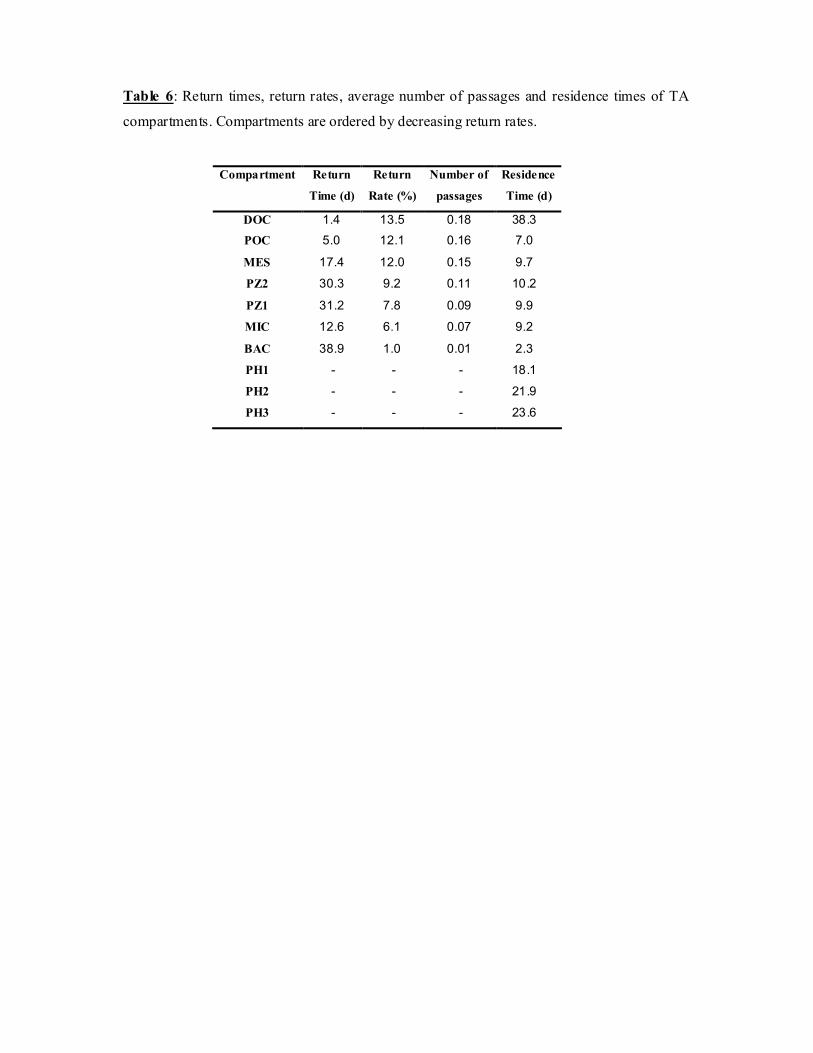
Table 6: Return times, return rates, average number of passages and residence times of TA

compartments. Compartments are ordered by decreasing return rates.

Compartment Return

Time (d)

Return

Rate (%)

Number of

passages

Residence

Time (d)

DOC 1.4 13.5 0.18 38.3 POC 5.0 12.1 0.16 7.0

MES 17.4 12.0 0.15 9.7

PZ2 30.3 9.2 0.11 10.2

PZ1 31.2 7.8 0.09 9.9

MIC 12.6 6.1 0.07 9.2

BAC 38.9 1.0 0.01 2.3

PH1 - - - 18.1

PH2 - - - 21.9

PH3 - - - 23.6

Table 7: Return times, return rates, average number of passages and residence times of PB

compartments. Compartments are ordered by decreasing return rates. The return times are

given in days.

Compartment Return

Time (d) Return

Rate (%) Number of passages

Residence Time (d)

3XXX 46 60.8 4.0 73.8XX

2XXX 55 59.5 3.6 107.1XX

4XXX 37 55.9 2.9 48.8XX

14XXX 20 51.3 2.2 29.8XX

13XXX 23 51.1 2.1 33.1XX

8XXX 36 49.8 2.0 33.2XX

12XXX 54 49.3 1.9 61.1XX

7XXX 30 46.8 1.7 26.2XX

10XXX 28 43.7 1.4 19.7XX

1XXX 50 38.2 1.0 157.1XX

15XXX 64 34.4 0.8 27.8XX

11XXX 35 33 0.7 111.1XX

5XXX 65 13.5 0.2 45.7XX 6XXX 51 12.3 0.2 55.8XX

9XXX - 0 0.0 23.1XX

Figure captions

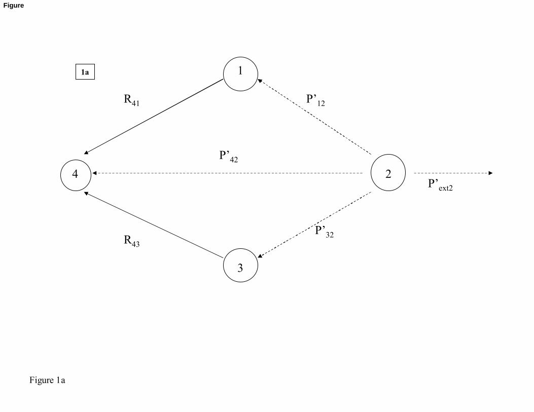
Figure 1: Theoretical example used for the explanation of the indices computation. This

example counts 4 compartments, which can be compartments of a trophic web: 1 for

phytoplankton, 2 for bacteria, 3 for detritus and 4 for zooplankton.

Figure 2: Presentation of the two case studies. 2a) Graph of Takapoto ecological network

(Niquil et al., 2001). PH1: cyanobacteria, assimilated to phytoplankton < 1 µm, PH2:

picoeukaryotes, or phytoplankton from 1 to 3 µm, PH3: phytoplankton > 3 µm, BAC:

heterotrophic bacteria, PZ1: protozoa < 35 µm, PZ2: protozoa > 35 µm, MIC: metazoan

zooplankton < 250 µm, MES: metazoan zooplankton > 250 µm, DOC: detritus (non living

carbon > 0.7 µm), POC: dissolved organic carbon (< 0.7 µm). 2b) Boundaries of the 16

regions of Passamaquody Bay. Region 16 represents the adjacent open ocean and is an

absorbing boundary state for the Markov Chain (Thompson et al. 2002).

Figure 3: Probability that a particle leaving a source compartment has reached the target

compartment in TA model after the time delay given in abscissa (in days). Figure 3a

represents the strong pairs: (PH3, DOC) (fast) and (PH3, BAC) (slow), and Figure 3b

represents the weak pairs: (BAC, MES) (fast) and (MES, MIC) (slow). See Figure 2a for the

abbreviations.

Figure 4: Probability that a particle leaving a source compartment has reached the target

compartment in PB model after the time delay given in abscissa (in days). Figure 4a represent

the strong pairs: (6, 8) (fast) and (1, 10) (slow), and Figure 4b represents the weak pairs: (13,

12) (fast) and (1, 5) (slow). The region numbers are given in Figure 2a.

Figure 5: Representation of transfer rate vs. transit times for TA pairs. The space can be

divided into various regions: low/mean/strong pairs according to the value of the transfer rate,

and slow/fast couple according to the value of the transit times. See Figure 2a for the

abbreviations.

Figure 6: Integrated network based on strong and mean links between compartments of TA

model. The strong links are represented in bold, fast ones in lines, and slow ones in dashed

lines. In Figure 6a, all the mean links are represented in dotted lines (see Figure 2a for the

abbreviations). Figure 6b represents the simplified network, and only the mean fast links are

represented in dotted lines.

Figure 7: Integrated network based on strong and mean links between compartments of PB

model. The strong links are represented in bold, fast ones in lines, and slow ones in dashed

lines. In Figure 7a, all the mean links are represented in dotted lines. Figure 7b represents the

simplified network, and only the mean fast links are represented in dotted lines.

1

3

24

P’12

P’42

P’32

R41

R43

P’ext2

1a

Figure 1a

Figure

1

3

24

P’12

P’42

P’32

R21

R24

R23

P’ext2

1b

Figure 1b

Figure 2a

PH1

PH3

PH2

POC

PZ2

PZ1

MESMIC

BAC

DOC

Figure 2b

1

2

3

4

5 6

78

9

10

11

12

13

14

1516

Figure 3a

0 50 100 150 200 250 300 3500

0.1

0.2

0.3

0.4

0.5

time (d)

PH3;DOCPH3;DOC

Figure 3b

0 50 100 150 200 250 300 3500

0.01

0.02

0.03

0.04

time (d)

BAC;MICPOC;BAC

Figure 4a

0 100 200 3000

0.2

0.4

0.6

0.8

time (days)

(1;10)

(6;8)

Figure 4b

0 100 200 3000

0.05

0.1

time (days)

(1;5)

(13;12)

Figure 5

0 5 10 15 20 25 30 35 400

0.1

0.2

0.3

0.4

0.5

PH1;BAC

PH1;PZ1

PH1;PZ2

PH1;MIC

PH1;MES

PH1;DOC

PH1;POC

PH2;BACPH2;PZ1

PH2;PZ2

PH2;MIC

PH2;MES

PH2;DOC

PH2;POC

PH3;BAC

PH3;PZ1

PH3;PZ2

PH3;MIC

PH3;MES

PH3;DOC

PH3;POC

BAC;PZ1BAC;PZ2BAC;MIC

BAC;MES

BAC;DOC

BAC;POC

PZ1;BAC

PZ1;PZ2

PZ1;MIC

PZ1;MES

PZ1;DOC

PZ1;POC

PZ2;BAC

PZ2;PZ1

PZ2;MIC

PZ2;MES

PZ2;DOC PZ2;POC

MIC;BACMIC;PZ1

MIC;PZ2

MIC;MES

MIC;DOC

MIC;POC

MES;BAC

MES;PZ1

MES;PZ2

MES;MIC

MES;DOC

MES;POC

DOC;BAC

DOC;PZ1

DOC;PZ2

DOC;MIC

DOC;MES

DOC;POC

POC;BACPOC;PZ1

POC;PZ2

POC;MIC

POC;MES

POC;DOC

Transit time

Tran

sfer

Rat

estrong

fast slow

weak

Figure 6a

PH1

PH3

PH2

POC

PZ2

PZ1

MESMIC

BAC

DOC

strong fast

strong slow

mean

Figure 6b

PH

POC

PZ

MIC

BAC

DOC

strong fast

strong slow

mean

Figure 7a

1

2

3

4

56

7

8

13

11

12

15

14

10

9

strong fast

strong slow

mean

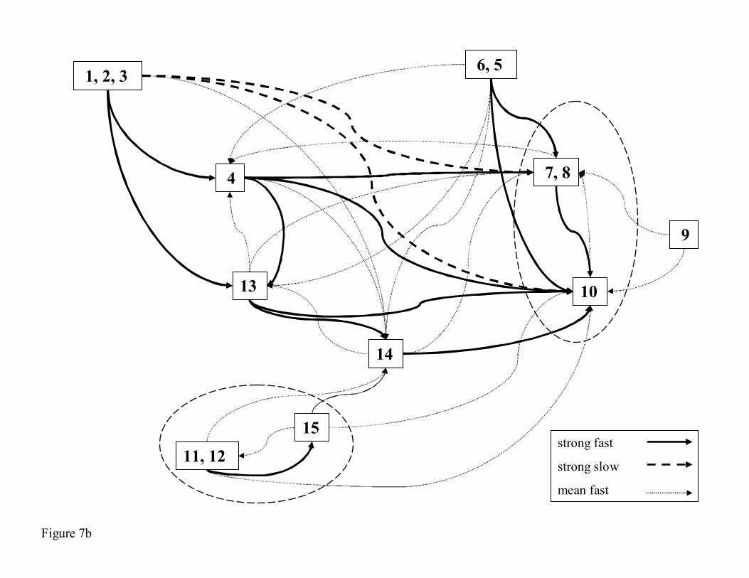
Figure 7b

1, 2, 3

4

6, 5

7, 8

13

11, 12

15

14

10

9

strong fast

strong slow

mean fast