Chlorination Disinfection By-Products (DBPs) in Drinking Water and Public Health in Canada

A Primer for

Public Health Practitioners Reviewing Evidence from over 30 Years of Research

A Knowledge Translation Review

for the

National Collaborating Centre on Environmental Health

by

Steve E. Hrudey, FRSC, FSRA, DSc (Eng), PhD, PEng

Professor Emeritus

University of Alberta Edmonton, Alberta

2008

Production of this report has been made possible through a financial contribution from the Public Health Agency of Canada through the National Collaborating Centre for Environmental Health. The views expressed herein do not necessarily represent

the views of the Public Health Agency of Canada or the National Collaborating Centre for Environmental Health.

ii

iii

i

Executive Summary

The challenge of judging and managing any public health risks “caused by” chlorination disinfection by-products (DBPs) in drinking water is likely the most complex issue that has faced the drinking water industry in the developed world over the past 3 decades. However, public health professionals must be acutely aware of the massive toll of death and illness occurring worldwide from contamination of drinking water by microbial pathogens. Likewise, the drinking water disease outbreaks in Walkerton and North Battleford reminded Canadians that microbial contamination of drinking water is a pervasive risk which can cause disease and death if there is ever a failure to maintain effective control of pathogens in drinking water. Consequently, public health health professionals must be very sure that any efforts at being precautionary in managing DBP risks are never allowed to compromise necessary measures to prevent the ever-present threat of waterborne disease. A major portion of the complexity of the chlorination DBPs issues arises from the inherent limitations of our primary scientific approaches to studying the problem, toxicology and epidemiology. These limitations make it clear that only an integrated combination of evidence from toxicology and epidemiology can provide meaningful predictions for human health risk assessment. When the limitations of the methods available for investigation of health effects are taken together with the complexity of DBP chemistry (over 600 DBPs identified and countless numbers as yet unidentified), it is not surprising that obtaining clear and unambiguous answers about public health risk has not been easy. This primer provides a review of relevant strengths and limitations of epidemiology, toxicology and risk assessment for judging evidence of possible health effects of chlorination DBPs. The epidemiological and relevant toxicological evidence regarding risks of cancer and adverse reproductive outcomes has been summarized and briefly analyzed. The resulting challenges for risk management decision-making have been reviewed. There has been a rich history regarding chlorination DBPs and health risk. Chloroform, as the major trihalomethane (THM) in particular, has come full circle from being a chemical that was widely used in consumer products when its presence in drinking water as a chlorination DBP was first reported in 1974, to being a labelled a carcinogen in 1976 followed by bans on chloroform usage in various consumer products. The initial classification of chloroform as a carcinogen led to expectations that chlorination DBPs would prove carcinogenic in drinking water. In the meantime, testing of chloroform failed to reveal genotoxic properties and our understanding of the effect of experimental methods on the observed outcomes in rodent cancer bioassays had improved to the point that, by 1998, the U.S. EPA was prepared to accept that there was a threshold for chloroform carcinogenesis. Specialists who have been following this issue closely will be aware that chloroform is not expected to cause human cancer at or below the levels that are currently mandated for drinking water, depending on the method pursued and values assumed, very different risk estimates result. That perspective about the absence of a

ii

cancer risk from chloroform via drinkgin water exposure is not commonly understood among water professionals. In 2006, the Canadian MAC for total trihalomethanes (THM4) was subsequently re-affirmed at 100 µg/L, by the Federal-Provincial-Territorial Committee on Drinking Water recognizing that given all the uncertainties, there was essentially a negligible difference in public health risk between a MAC of 80 µg/L vs. 100 µg/L. The final MAC for THM4 is certainly precautionary for any cancer risk posed specifically by THM4. Contrary to some critical perceptions among public health practitioners, the final choice of the 100 µg/L MAC was not simply justified only on the economic grounds of what MAC that water providers can afford to meet. An expert panel review convened by Health Canada in 2002 agreed that the available health evidence did not justify a MAC different from 100 µg/L For public health professionals, it is important to recognize no matter which evidence or interpretation may be preferred, the level of precaution for THM4 based on toxicology evidence is very large. Exceeding MAC values for chloroform and bromodichloromethane (BDCM) by less than a factor of 10 would certainly not call for emergency actions based on any expectation of adverse health outcomes. Of course, public pressure for decisive action in such circumstances presents a different reality. At present, a causal link between bladder cancer and some component of chlorine disinfected drinking water remains a working hypothesis with various elements of support primarily from the number of epidemiologic findings. Overall, the consistency of findings on urinary bladder cancer is notable, but the specificity and plausibility, as to causal agent, are weak to negative and the strength of association is generally low enough to be susceptible to even minor confounding. The recent regulatory focus on THMs has been rationalized, in large part, as providing a means to reduce the occurrence of bladder cancer. Unfortunately, the evidence suggests that there is no causal connection between THMs and bladder cancer which means that reducing THMs alone cannot be assured to achieve any reduction in population bladder cancer. If there are other chlorination DBPs that are responsible for causing bladder cancer, reduction of THMs may or may not reduce these other chlorination DBPs. Only mitigative measures such as reduction of chlorination DBP precursors are likely to assure concurrent reduction of THMs and the unknown chlorination DBPs. Other measures specifically targeting reduced THM formation, such as aeration or chloramination, may not achieve any reduction of the unknown chlorination DBPs and, in the case of chloramination, may yield an increase in other more toxic chlorination DBPs, such as nitrosamines. More focused attention on causes of bladder cancer is necessary because a large proportion of the comparisons of high chlorination DBP exposures with lower chlorination DBP exposures involve comparing exposure to disinfected surface water vs. lightly or non-disinfected groundwater. The possibility of chlorination DBPs causing adverse reproductive outcomes was largely one of academic and research interest before the publication of the Waller et al. 1998

iii

study. Numerous previous studies had found suggestive, but inconsistent and usually not significant associations of a variety of adverse birth outcomes with chlorination DBPs. The large size and comparative strength of the prospective cohort study reported by Waller et al. (1998) drew justifiable attention to the reported significant association of spontaneous abortion with THM4 and even more strongly with BDCM exposure. There was a compelling need to confirm whether chlorination DBPs could possibly cause adverse health effects based on short-term (i.e. daily peak) exposures rather than the long-term chronic exposures of concern for bladder cancer (generally greater than 40 years of exposure needed for elevated risk). Evidence for adverse reproductive outcomes has been inconsistent at best, with evidence for birth defects caused by chlorination DBPs being primarily negative. The case for a causal association of spontaneous abortion with chlorination DBPs has not been supported by the most thorough study to date on this subject. The current state of knowledge on causation of adverse reproductive outcomes provides no basis for any tightening of current MAC values for chlorination DBPs. Given the inevitable uncertainties, drinking water professionals need to view the subject of DBPs and public health as a major issue that must continue to be managed in a precautionary manner. This should be accepted even though over 30 years of health-related research into DBPs in drinking water appears to warrant an over-all rating of the evidence as indicating that there is no “certain” health effect that has been proven between any DBP within currently regulated levels and any specific health outcome. Although there is no substantive health effects evidence to support continued reduction of the levels for currently regulated DBPs, the possibility of there being some causal association between some specific DBPs and adverse health effects remains a viable hypothesis. It is necessary to maintain a sensible, precautionary approach to managing DBPs that recognizes that it is at least as likely that there may no adverse health effects from current disinfection practices as it is that future research may be able to establish a more certain causal relationship for one or more DBPs and specified outcomes. The bottom line for public health practitioners who recognize the importance of maintaining their credibility is to justify the case for control of chlorination DBPs in drinking water on a position of reasonable precaution. For most circumstances likely to be encountered in Canada, there is no need, nor justification provided by the evidence, to advocate taking urgent or extreme action on chlorination DBPs based on a realistic expectation of adverse health outcomes. Experienced public health practitioners know how difficult it can be to motivate the public to take responsible actions even when there is a true imminent danger known from strong causal evidence (i.e. immunization against infectious disease outbreaks). The credibility of public health practitioners for advocating substantial action for public health protection needs to be used judiciously.

iv

Table of Contents Executive Summary i Table of Contents iv List of Tables vii List of Figures viii Glossary of Acronyms x 1. INTRODUCTION 1 1.1 Purpose and Terminology 1

1.1.1 Purpose 1 1.1.2 Terminology 1 1.2 Current Status of Drinking Water Chlorination Disinfection 2

By-Products in Canada

1.3 Historical Perspective 4

1.4 Technical Background 6 1.4.1 Classes of Well Known Chlorination DBPs 6 1.4.2 Physical and Chemical Properties of DBPs 8 1.4.3 Formation of DBPs in Drinking Water 9 1.4.4 Recent and Emerging DBPs 10 1.5 Public Health Risk Assessment and Risk Management 13 1.5.1 Overview 13 1.5.2 Hazard Identification and Assessing Evidence 14 1.5.3 Assessing Exposure 23 1.5.4 Quantifying Risk 25 1.5.5 Characterizing Risk 30 1.5.6 Decision-making and Implmentation of Risk Management 32

2. CHLORINATION DISINFECTION BY-PRODUCTS AND CANCER 34 2.1 Toxicology Evidence from Long Term Studies on Cancer 34 2.1.1 Chloroform 34 2.1.2 Bromodichloromethane 36 2.1.3 Haloacetic acids 37

2.2 Epidemiology Evidence on Cancer 38 2.2.1 Colon Cancer 39 2.2.2 Rectal Cancer 41 2.2.3 Urinary Bladder Cancer 43

v

3. CHLORINATION DISINFECTION BY-PRODUCTS AND ADVERSE 50 REPRODUCTIVE OUTCOMES

3.1 Toxicology Evidence on Adverse Reproductive Outcomes 50 3.1.1 Chloroform 50 3.1.2 Bromodichloromethane 50 3.1.3 Haloacetic acids 51 3.1.4 Other Chlorination DBPs 51 3.2 Epidemiology Evidence on Adverse Reproductive Outcomes 52

in Relation to Chlorination DBP Exposure 3.2.1 Spontaneous Abortion 52 3.2.2 Still Birth 56 3.2.3 PreTerm Delivery 58 3.2.4 Low Birth Weight, Very Low Birth Weight & 58

Term Low Birth Weight 3.2.5 Intrauterine Growth Retardation and Small for Gestational Age 58 3.2.6 Birth Defects 66 4. PUBLIC HEALTH RISK MANAGEMENT AND UNCERTAINTY 74

4.1 Characterization of Uncertainty 75 4.1.1 Variability 75 4.1.2 Knowledge or True Uncertainty 75 4.1.3 Type 1, 2, 3 Errors 75

4.2 Risk Management Options 78 4.3 The Public in Public Health Risk Management 78 5. DISCUSSION AND CONCLUSIONS 83 5.1 Discussion 83 5.2 Conclusions 90 6. ACKNOWLEDGEMENTS 92 7. REFERENCES CITED 93 8. APPENDICES 106

A1 LONG TERM CANCER STUDIES 107

vi

A2 CANCER EPIDEMIOLOGY 116 A3 REPRODUCTIVE TOXICOLOGY 141 A4 ADVERSE REPRODUCTIVE EFFECTS EPIDEMIOLOGY 154

vii

List of Tables Table 1 DBP Regulations and Guidelines 3 Table 2 Classes of Established Chlorination DBPs 7 Table 3 Disinfectants and Resulting Major DBPs 8 Table 4 Recently Found and Emerging DBPs 11 Table 5 Comparison of Observational Epidemiology with Experimental 83 Toxicology for Yielding Human Risk Assessment Insights Table 6 1 Day Exposure Health Advisory Level 85 Appendix A1 106 Table A1-1 Long Term Cancer Studies on Chloroform 107 Table A1-2 Long Term Cancer Studies on Bromodichloromethane (BDCM) 112 Table A1-2 Long Term Cancer Studies on Haloacetic Acids (HAAs) 116 Appendix A2 118 Table A2-1 Epidemiology Studies of Cancer Sites Other Than Bladder, 119 Colon or Rectum Table A2-2 Epidemiology Studies Including Colon and/or Rectal Cancer 125 Table A2-3 Epidemiology Studies Including Bladder Cancer 134 Appendix A3 144 Table A3-1 Reproductive Toxicology Studies on Chloroform by Ingestion 145

or Intraperitoneal Injection

Table A3-2 Reproductive Toxicology Studies on Chloroform by Inhalation 147 Table A3-3 Reproductive Toxicology Studies on BDCM by Ingestion 149 Table A3-4 Reproductive Toxicology Studies on Haloacetic Acids by Ingestion 154 Appendix A4 157 Table A4-1 Epidemiology Studies on Adverse Reproductive Outcomes 158

viii

List of Figures Figure 1 Basic 2 x 2 Table for Epidemiologic Analysis 16 Figure 2 Exposure Pathways for Chemicals in Tapwater 24 Figure 3 NOAEL and LOAEL on a Dose – Response Curve 26 Figure 4 Association Between Cancer Slope Factors and Maximum 27 Tolerated Dose (MTD) Used in Rodent Carcinogen Bioassays Figure 5 Explanation of Remarkably Strong Association 28 Between CSF and MTD Figure 6 Summary of Analytical Epidemiology Evidence on Colon Cancer 40 and Exposure to Chlorination DBPs Figure 7 Summary of Analytical Epidemiology Evidence on Rectal Cancer 42 and Exposure to Chlorination DBPs Figure 8 Summary of Analytical Epidemiology Evidence on Urinary Bladder 44

Cancer and Exposure to Chlorination DBPs Figure 9 Summary of Analytical Epidemiology Evidence on 55

Spontaneous Abortion and Exposure to Chlorination DBPs

Figure 10 Summary of Epidemiology Evidence on Stillbirth and 57 Exposure to Chlorination DBPs Figure 11 PreTerm Delivery and Exposure to Chlorination DBPs 60 Figure 12 Summary of Epidemiology Evidence on Low Birth Weight 61 and Exposure to Chlorination DBPs Figure 13 Summary of Epidemiology Evidence on Very Low Birth Weight 62 and Exposure to Chlorination DBPs Figure 14 Summary of Epidemiology Evidence on Term Low Birth Weight 63 and Exposure to Chlorination DBPs Figure 15 Summary of Epidemiology Evidence on Intrauterine Growth 64 Retardation and Exposure to Chlorination DBPs Figure 16 Summary of Epidemiology Evidence on Small for Gestational 65 Age and Exposure to Chlorination DBPs

ix

Figure 17 Summary of Epidemiology Evidence on All Birth Defects and 67 Exposure to Chlorination DBPs Figure 18 Summary of Epidemiology Evidence on Cardiovascular 68 Anomalies and Exposure to Chlorination DBPs Figure 19 Summary of Epidemiology Evidence on Cleft Defects and 69 Exposure to Chlorination DBPs Figure 20 Summary of Epidemiology Evidence on CNS Anomalies 70 Including Neural Tube Defects and Spina Bifida with Exposure to Chlorination DBPs Figure 21 Summary of Epidemiology Evidence on Urinary Tract Defects with 72 Exposure to Chlorination DBPs Figure 22 Summary of Epidemiology Evidence on Respiratory Defects with 73 Exposure to Chlorination DBPs

x

Glossary of Acronyms AbWl abdominal wall defects BAC biological activated carbon BDCM bromodichloromethane BDef birth defects (general) BW body weight (mass) CAn congenital anomalies CdAn cardiac anomalies CDBM chlorodibromomethane CDBPs chlorination disinfection by-products (NOT chlorinated DBPs) ChAb chromosomal abnormalities ClDef cleft defects ClPal cleft palate CNS central nervous system CNSAn central nervous system anomalies CR contact rate CSF cancer slope factor CH chloral hydrate CI confidence interval CP chloropicrin CPh chlorophenols CSn Caersarian section CV cardiovascular DBA dibromoacetic acid DBPs disinfection by-products DCAA dichloroacetic acid DCAN dichloroacetonitrile DnSyn Down syndrome EHPs environmental health practitioners ECD electron capture detector EDF Environmental Defence Fund ER excess lifetime cancer risk ER(d) excess lifetime cancer risk at specified daily average lifetime dose FDth fetal death FPTCDW federal/provincial/territorial committee on drinking water GAC granular activated carbon GCDWQ Guidelines for Canadian Drinking Water Quality GLP good laboratory practice HAA5 haloacetic acids (most common) HAA9 haloacetic acids (all possible chlorinated and brominated acetic acids) HAN haloacetonitrile HK haloketones HOBr hypobromous acid Hyceph hydrocephalus Hyp hypospadias

xi

KH Henry’s Law constant (air / water partition coefficient) KOW octanol / water partition coefficient IARC International Agency for Research on Cancer ICPS International Programme on Chemical Safety IUGR intrauterine growth retardation LBth live birth LBWt low birth weight LC50 lethal concentration to 50% of exposed population (median lethal

concentration) LD50 lethal dose to 50% of exposed population (median lethal dose) LMS linearized multistage model LOAEL lowest observed adverse effect level MAC maximum acceptable concentration (Canadian guidelines) MBA monobromoacetic acid MCdAn major cardiac anomalies MCL maximum contaminant level (U.S. regulations) MCLG maximum contaminant level goal MSD mass selective detector (mass spectrometry detector) MTD maximum tolerated dose MX 3-chloro-4-(dichloromethyl)-5-hydroxy-2(5H)-furanone (for other

halogenated furanones see Table 3) NCCEH National Collaborating Centre for Environmental Health NCI National Cancer Institute (U.S.) NDMA nitrosodimethylamine NnDth neonatal death NnJd neonatal jaundice NOAEL no observed adverse effect level NOM natural organic matter NS nervous system defect NTDef neural tube defects NTP national toxicology program OCf oral clefts OfCf orofacial clefts OR odds ratio PAR population attributable risk P/CCRARM Presidential / Congressional Commission on Risk Assessment and Risk

Management pH negative logartithm of hydrogen ion concentration PTm pre-term q1* upper 95% limit on the cancer slope factor (CSF) using the LMS

(linearized multistage model) RenFef renal defects RfD reference dose RR rate ratio, relative risk RsDef respiratory defects RSD risk specific dose

xii

SA source allocation factor SB spina bifida SDWA Safe Drinking Water Act SmBL small body length SmCrC small cranial circumference SpAb spontaneous abortion StBth still birth SGA small for gestational age TBROM total brominated THMs TCAA trichloroacetic acid TDI tolerable daily intake THM, THM4 trihalomethanes, total trihalomethanes TOC total organic carbon TOX total organic halide UF uncertainty factor UrTrDef urinary tract defects U.S. EPA U.S. Environmental Protection Agency U.S. PHS U.S. Public Health Service UV ultraviolet radiation VLBWt very low birth weight VSDef ventricular septal defects WHO World Health Organization

1

1. INTRODUCTION 1.1 Purpose and Terminology 1.1.1 Purpose The National Collaborating Center for Environmental Health (NCCEH) aims to be an indispensable resource for environmental health practitioners and policy-makers across Canada by engaging in the synthesis, translation and exchange of knowledge about relevant environmental health issues. This review was undertaken to address the NCCEH mandate regarding the public health risk management of chlorination disinfection by-products in drinking water in Canada. The necessary pre-eminence of adequate disinfection to prevent waterborne disease over satisfying compliance with maximum acceptable concentration (MAC) guideline values for various disinfection by-products (DBPs) is acknowledged in the Guidelines for Canadian Drinking Water Quality (GCDWQ) and various provincial regulatory measures. However, the rationale for managing those DBPs that currently have MACs, and the nature, quality and certainty of evidence upon which those MACs are derived have not been systematically reviewed in a manner that will allow environmental health practitioners to perform effective public health risk management. There is empirical evidence that fear of health risks from DBPs has led to compromised disinfection resulting in waterborne disease outbreaks. Environmental health practitioners (EHPs) must deal with various specific situations where a drinking water system fails to comply with one or more DBP MACs. The question of what actions are appropriate to protect public health in such circumstances can be expected to arise with growing frequency. While there is an enormous body of literature available on various aspects of health risks for individual DBPs, there is limited useful and practical guidance about the nature of health risk evidence for specific DBPs in relation to other risks in public health practice. EHPs need guidance in developing effective risk management measures to resolve a compliance problem without compromising disinfection for individual water systems that are occasionally or chronically exceeding DBP MAC values. Likewise, there is nothing useful for developing a risk communication strategy to address the immediate and short term risk management measures while longer term risk management solutions are being developed. 1.1.2 Terminology In this document, disinfection by-product (DBP) refers to any chemical substance that is unintentionally produced as a by-product of a disinfection process, most commonly by means of a reaction between the disinfectant and naturally occurring organic matter (NOM) found in drinking water. This document is limited in scope to the most common disinfection by-products which have received the greatest public health-relevant attention in Canada. Collectively, these will be termed “chlorination disinfection by-products”. Other publications related to this topic have used the acronym CDBP, but this report will avoid that acronym. DBP will be used where use of the acronym is more practical than spelling out the whole word. The reason for avoiding use of CDBPs is the possible confusion between “chlorination

2

disinfection by-products” and “chlorinated disinfection by-products”, a term that CDBPs has been equated with in other publications. The term “chlorination DBPs” refers to any DBPs produced by a chlorination or related chlorine (e.g. chloramination) disinfection process. Chlorinated DBPs, taken literally, includes only those DBPs that contain chlorine. This restriction is problematic for two reasons, chlorination produces some disinfection by-products that are halogenated, but may not contain any chlorine, i.e. bromoform, one of the compounds included in trihalomethanes (THM), the first DBPs to be subject to guideline or regulation. Furthermore, and this is not as widely recognized, chlorination produces numerous by-products that contain no halogens, e.g., aldeyhydes and nitrosamines. These issues will be elaborated in Section 1.4, but the public health relevance is that there is no need for any DBP to contain chlorine or any other halogen for them to pose a public health concern. For example, some specific nitrosamines are substantially (~1,000 fold) more potent as carcinogens than any of the THMs. Consequently, it is essential that any public health-relevant discussion of DBPs arising from the chlorination process includes DBPs regardless of whether they contain chlorine or any other halogen. Chlorination DBPs, as used in this review, also does not include any of the inorganic DBPs such as chlorite, chlorate and bromate that may be formed by various alternative disinfectants (e.g. chlorine dioxide, ozone) Other terminology to be clarified at the outset is the use of THM4, HAA5 and HAA9. The literature on DBPs includes many papers that refer to TTHM as well as THM. TTHM is intended to mean total trihalomethanes, as distinct from any of the individual THMs, chloroform, bromodichloromethane (BDCM), chlorodibromomethane (CDBM) or bromoform. Because TTHM is confusing in relation to THM as they should mean the same thing, this report will use the term THM4 to refer to any data that represents the total THM content (i.e. a sum of all 4 THMs). Similarly, HAA5 and HAA9 represent total summed analyses for haloacetic acids. HAA5 represents the summed total of monochloracetic acid, dichloroacetic acid, trichloroacetic acid, bromoacetic acid and dibromoacetic acid. HAA5 is the combination of haloacetic acids that are regulated with a maximum contaminant level (MCL) under the U.S. Safe Drinking Water Act. HAA9 represents the sum total of all possible chlorinated and brominated haloacetic acids.

1.2 Regulation of Drinking Water Chlorination DBPs in Canada and Other

Countries Background technical details, including chemical description of chlorination DBPs, are provided in Section 1.4. Canada was the first to specify a limit for THMs, setting a drinking water quality guideline in 1978. The U.S. EPA set a regulatory limit for THMs in 1979. They introduced the concept of regulating THMs as a running annual average over a 1 year period, a concept that was adopted for THMs in Canada in 1992 (officially in 1996) and which remains in current use.

3

Limits have later appeared for haloacetic acids, either as a group (HAA5) in the U.S. and Canada, or individually in Australia and with the WHO and additional DBP limits have been adopted (HAA5 in 2008) or are proposed in Canada Canada set a very low guideline for bromodichloromethane (BDCM) in 2006, at 16 µg/L, compared with the WHO guideline of 60 µg/L. The Canadian guideline is now being reconsidered on the strength of new evidence indicating that BDCM is not carcinogenic via drinking water exposure (Section 2.1.3). Table 1 Chlorination DBP Regulations and Guidelines Source Chlorination

Disinfection By-Product Guideline

Value (µg/L)

Year Set or renewed

Australia THM4 (maximum) 250 1996, 2004 monochloroacetic acid 150 2004 dichloracetic acid 100 2004 trichloroacetic acid 100 2004 cyanogen chloride 80 2004 chloral hydrate (trichloroacetaldehyde) 20 2004 Canada - MAC THM4 (maximum) 350 1978 THM4 (running annual average) 100 1996, 2006 bromodichloromethane (BDCM)a 16 2006 HAA5 (maximum) 80 2008 USA - MCL THM4 (running annual average) 100 1979 THM4 (running annual average) 80 1998 HAA5 (annual average) 60 1998 WHO chloroform 30 1984 chloroform 200 1993, 2004 bromodichloromethane (BDCM) 60 2004 chlorodibromomethane 100 2004 bromoform 100 2004 choral hydrate 10 2004 cyanogen chloride 70 2004 dibromoacetonitrile 70 2004 dichloroacetic acid 50 2004 dichloroacetonitrile 20 2004 monochloroacetic acid 20 2004 trichloroacetic acid 200 2004 a Under review based on new evidence showing lack of carcinogenicity for BDCM

4

1.3 Historical Perspective Dramatic changes arose in the 1970s for the drinking water industry in developed countries. At the start of that decade, public health and sanitary engineering courses were taught as if all knowledge needed for safe drinking water was already in hand; academic research into drinking water quality or safety had a lower profile compared with wastewater treatment or water pollution research. The combination of coagulation, filtration and disinfection, mainly by chlorination, was generally considered full and sufficient treatment for drinking water. Process performance optimization was not a common priority In the late 1960s and early 1970s, trace organic analysis with gas chromatography, linked to electron capture and mass spectrometry detection (ECD and MSD), began to dramatically improve analytical sensitivity resulting in the detection of numerous trace organic compounds in treated drinking water supplies. These advances profoundly altered public and professional perceptions of drinking water quality and safety. In the U.S., a study for the Environmental Defense Fund (EDF) suggesting cancer mortality for those consuming treated drinking water from the Mississippi River was higher than for those consuming drinking water from groundwater sources attracted enormous attention . This was reinforced by a U.S. EPA report within the same week that the New Orleans water supply drawn from the Mississippi River contained a number of trace organics, many of which were suspected carcinogens USEPA 1974. Coincidently, these events preceded by only five days a House of Representatives vote on the new Safe Drinking Water Act, providing a vote margin of 296 to 85, sufficient to override a threatened Presidential veto Marx 1974. On December 16, 1974, the President signed the Safe Drinking Water Act (SDWA) into law, including a specific requirement for the U.S. EPA to conduct a national survey of municipal water supplies for the presence of halogenated organics. Meanwhile, in Europe, Johannes Rook 1974 had already reported that chloroform and the other THMs were found at higher concentrations in chlorinated drinking water than in raw surface water supplies. He provided meticulous evidence for his hypothesis that the THMs were produced by reactions between chlorine and naturally occurring organic matter in water. Rook’s discovery, made years earlier using his experience analyzing volatile flavour components in beer, was soon corroborated by Bellar et al. 1974 and in the national survey of halogenated organics mandated by the SDWA (Symons 1975). They also found higher levels of THMs with increasing chlorine contact during disinfection. An insider account of the emergence of disinfection by-products as a drinking water issue has been documented by Jim Symons, who headed the relevant U.S. EPA research program at that time Symons (2001a, b). Shortly after the growing body of evidence showing chloroform in chlorinated drinking water supplies, the National Cancer Institute (NCI) published results of a rodent cancer bioassay on chloroform (NCI 1976). The evidence from these rodent bioassays showing kidney tumours in rats and liver tumours in mice led to chloroform, the main THM,

5

being declared a suspected human carcinogen. The U.S. Food and Drug Administration quickly banned its use in cosmetics. This was a dramatic change for chloroform which had been widely used as an anaesthetic from the mid 1800s into the early 1900s. Ironically, Dr. John Snow, the public health icon who established with epidemiologic evidence that fecal contaminated drinking water was responsible for cholera epidemics in London, made his livelihood practicing as an anaesthetist primarily using chloroform (Vinten-Johansen et al. 2003). The U.S. SDWA requires development of a maximum contaminant level goal (MCLG) for regulated drinking water contaminants. The MCLG is the maximum level of a contaminant in drinking water at which no known or anticipated adverse health effects would occur, and which allows an adequate margin of safety. A maximum contaminant level (MAC) is the highest level of a contaminant that is allowed in drinking water. MCLs are set as close to MCLGs as feasible using the best available treatment technology and taking cost into consideration. MCLs are enforceable standards. U.S. EPA policy for carcinogens in drinking water had specified a MCLG of zero (reflecting a default assumption that there is no threshold for the action of carcinogens). However, mounting toxicological evidence on the mode of action of chloroform clearly demonstrated a threshold mechanism for carcinogenic effects. This resulted in a U.S. EPA expert review panel recommending the abandonment of the MCLG of zero and replacement with a limit based on an estimated threshold. Thus in 1998, the U.S. EPA proposed to raise the MCLG to 300 µg/L in accordance with this expert advice. However, the U.S. EPA Final Rule withdrew the proposal to change the MCLG for chloroform from zero as many intervenors protested this precedent-setting measure (Pontius 2000). The Chlorine Chemistry Council sought a court review of the U.S. EPA decision as the Safe Drinking Water Act requires the U.S. EPA to use the best available science in setting standards and regulations. Although the U.S. EPA acknowledged that the best available science called for raising the MCLG above zero, it had nevertheless decided to retain the zero MCLG. On March 31 2000, the U.S. District Court ruled that the U.S. EPA had violated the Safe Drinking Water Act by failing to use the best available science. The court found that the EPA action of setting the MCLG of chloroform at zero to be “arbitrary and capricious” and in excess of statutory authority. The U.S. EPA withdrew the zero MCLG in May 2000, subsequently replacing it with a MCLG of 70 µg/L. The lower MCLG (from 300 µg/L) was presumably based upon assigning a lower proportion of total human exposure to chloroform to ingestion of drinking water, thereby justifying a tighter limit for chloroform in drinking water. The changing fortunes of chloroform over the years illustrate some of the problems in risk management for DBPs in the presence of uncertainty and incomplete evidence, and the difficulty in revising entrenched regulatory measures as scientific knowledge improves.

6

1.4 Technical Background 1.4.1 Classes of Currently Known Chlorination Disinfection By-Products DBPs are, by definition, the result of a reaction between a disinfecting agent (chemical or physical) and a precursor chemical in the source water. Therefore, DBP formation will depend on factors such as the disinfectant used, the precursors present and the reaction conditions provided. Major classes of DBPs include halogenated organic compounds such as trihalomethanes, haloacetic acids, haloacetonitriles, chlorophenols, chloral hydrate and chloropicrin. Other non-halogenated DBPs reported include aldehydes, ketoacids, ketones, carboxylic acids, maleic acids, nitrosamines, alkanoic acids, benzene. Table 2 lists the individual DBP species of the various classes (adapted from Krasner et al. 1989, Froese et al. 1999). Trihalomethanes and haloacetic acids are the most prevalent compounds in chlorinated drinking water and form the largest groups in terms of quantity. Reported concentrations for trihalomethanes in drinking water supplies range from a minimum 3.1 μg/L to a maximum of 1280 μg/L and for haloacetic acids from <0.5 μg/L to 1230 μg/L (IPCS 2000). Reported ranges for other classes include:

Haloacetonitriles: (0.04 μg/L – 12 μg/L) Haloketones: (0.9 μg/L – 25.3 μg/L) Chlorophenols: (0.5 μg/L – 1 μg/L) Chloral hydrate: (1.7 μg/L – 3.0 μg/L) Chloropicrin: (<0.1 μg/L – 0.6 μg/L)

Although chlorination disinfection by-products have undergone the most investigation, it is important to recognise that all disinfectants will generate disinfection by-products since reaction mechanisms occur. Ozonation, for instance, produces a vastly different profile of disinfection by-products than chlorine, yielding oxygenated species such as bromate, iodate, chlorate, aldehydes and ketoacids rather than THMs, HAAs or HANs. Table 3 lists various disinfection by-products that have been determined for chlorine, chlorine dioxide, chloramine and ozone.

7

Table 2 Classes of Established Chlorination DBPs

DBP Class Individual DBPs Chemical Formula Trihalomethanes Chloroform CHCl3 THMs Bromodichloromethane CHCl2Br (collectively: THM4) Dibromochloromethane CHClBr2 Bromoform CHBr3 Monochloroacetic acid CH2ClCOOH Dichloroacetic acid CHCl2COOH Trichloroacetic acid CCl3COOH Haloacetic acids Bromochloroacetic acid CHBrClCOOH HAAs Bromodichloroacetic acid CBrCl2COOH (collectively: HAA9) Dibromochloroacetic acid CBr2ClCOOH Monobromoacetic acid CH2BrCOOH Dibromoacetic acid CHBr2COOH Tribromoacetic acid CBr3COOH Trichloroacetonitrile CCl3CN Haloacetonitriles Dichloroacetonitrile CHCl2CN HANs Bromochloroacetonitrile CHBrClCN Dibromoacetonitrile CHBr2CN Haloketones 1,1-Dichloroacetone CHCl2COCH3 HKs 1,1,1-Trichloroacetone CCl3COCH3 Miscellaneous Choral hydrate CCl3CH(OH)2 chlorinated organics Chloropicrin CCl3NO2 Cyanogen halides Cyanogen chloride ClCN Cyanogen bromide BrCN Chlorite ClO2

- Oxyhalides Chlorate ClO3

- Bromate BrO3

- Formaldehyde1 HCHO Aldehydes Acetaldehyde2 CH3CHO Glyoxal OHCCHO Methyl glyoxal CH3COCHO (odorous aldehydes) Isobutyraldehyde3 (CH3) 2CHCHO Isovaleraldehyde4 (CH3) 2CHCH2CHO 2-Methylbutyraldehyde5 (CH3)(C2H5)CHCHO Phenylacetaldehyde6 (C6H5)CH2CHO Glyoxalic acid OHCCHO Aldoketoacids Pyruvic acid CH3COCOOH Ketomalonic acid HOOCCOCOOH Carboxylic acids Formate HCOO- Acetate CH3COO- Oxalate OOCCOO-2 Maleic acids 2-tert-Butylmaleic acid HOOCC(C(CH3)3):CHCOOH Chlorophenols Chlorophenol C6H5Cl CPh Dichlorophenols C6H4Cl2 (odorous) Trichlorophenols C6H3Cl3 Chloroanisoles (odorous)

Trichloroanisoles7 CH3OC6H3Cl3

1formed from glycine 2formed from alanine 3formed from valine, Hrudey et al. 1988 4formed from leucine, Hrudey et al. (1988)

5formed from isoleucine, Hrudey et al. (1988) 6formed from phenyalanine, Hrudey et al. (1988)

7biotransformation of trichlorophenols

8

Table 3 Disinfectants and Resulting Major DBPs (adapted from ICPS 2000; UV added)

Disinfectant

Significant organohalogen DBPs

Significant inorganic DBPs

Significant non-halogenated DBPs

Chlorine

THMs, HAAs, HANs, CH, CP, CPh, N-chloramines, halofuranones, bromohydrins

chlorate (mostly from hypochlorite use)

aldehydes, cyanoalkanoic acids, alkanoic acids, benzene, carboxylic acids, nitrosamines

Chlorine dioxide

chlorite, chlorate

unstudied

Chloramine

HANs, cyanogen chloride, organic chloramines, CH, chloramino acids, haloketones

nitrate, nitrite, chlorate, hydrazine

aldehydes, ketones, nitrosamines

Ozone

bromoform, MBA, DBA, dibromoacetone, cyanogen bromide

chlorate, iodate, bromate, hydrogen peroxide, HOBr, epoxides, ozonates

aldehydes, ketoacids, ketones, carboxylic acids

Ultraviolet (UV)a major DBP production not yet identified

major DBP production not yet identified

major DBP production not yet identified

a research on DBPs from UV disinfection is limited, but to date, major DBP production has not been identified at UV doses used in water disinfection although UV irradiation is known to alter the chemical structure of NOM

1.4.2 Physical and Chemical Properties of DBPs The basic physical and chemical properties of individual compounds are important in determining their fate in water treatment processes, distribution systems and at the point of supply to consumers. An understanding of these properties is also needed for assessing the relative importance of the three potential human exposure routes (ingestion, inhalation, dermal absorption). Two important properties are the Henry’s Law Constant (KH) and the log Octanol – Water Coefficient (KOW). The value of the Henry’s Law Constant provides an indication of likely partitioning in air (i.e. a measure of volatility). The Log Octanol – Water Coefficient is a measure of the preference of the compound for the water phase (hydrophilic compounds) or the organic phase (lipophilic compounds). While ingestion is clearly relevant to all DBPs, only those which are volatile are significant in terms of inhalation exposure, while only lipophilic DBPs are likely to be absorbed through the skin.

9

Available data on KH and KOW for disinfection by-products is limited. However, values for trihalomethanes indicate that volatilization is significant for these compounds and that they are only slightly lipophilic, indicating that human exposure to these compounds is strongly influenced by inhalation/vapour-phase and dermal routes of exposure with activities such as bathing and showering being important. Haloacids are known to be very hydrophilic with negligible volatilization. Exposure to haloacids is therefore likely to be limited to ingestion of drinking water. Thus significantly different exposures to various DBPs from the same water supply will occur at an individual level depending on the varying water use activities undertaken by each person. 1.4.3 Formation of DBPs in Drinking Water Since the discovery of DBPs in drinking water there has been a concerted effort to understand how DBPs are formed and how they can be avoided. Most research was initially directed at THMs and variations on chlorination. Initially to avoid formation of THMs and other halogenated DBPs, alternative disinfectants were pursued and continued research has shown that varying levels and types of DBPs are produced by all disinfection methods and that DBPs may be reduced but not eliminated all together. The formation of DBPs in water treatment is influenced by several factors:

contact time disinfectant dose pH temperature total organic carbon (TOC) ultraviolet absorption (UV254) bromide

At the treatment plant, THMs and HAAs follow similar patterns of formation with rapid and curvilinear increases with both increasing contact time and increasing disinfectant dose. Both have shown rapid formation in less than 5 hours, with 90% being formed in the initial 24 hours and with concentrations levelling off after a prolonged period. Increasing contact time also increases concentrations of aldehydes providing a residual is present. Increase in disinfectant dose has a similar effect depending on the dose applied. Increasing pH tends to favour the formation of THMs (up to pH 9.5) and decrease formation of TCAA and TOX (Krasner 1999). Maximum concentrations of DCAA have been shown to occur at pH 7-7.5. For DBPs such as DCAN and trichloroacetone, higher formation occurs at low pH. Aldehydes, which form mostly through molecular ozone, indicate a negative effect with increasing pH with a 25% decrease in concentration for pH 7-8.5.

10

Generally, increasing temperature causes greater yield of DBPs (e.g. a change from 10 to 30°C produces a 15 – 25 % increase in concentration). Concentrations of THMs and HAAs also tend to increase for water higher in TOC and UV254. However the natural organic matter precursor character is important; humic acids are more reactive than fulvic acids. Aldehydes also show a positive effect with increasing TOC and UV254. The presence of the bromide ion shifts THMs and HAAs towards the more brominated species rather than the chlorinated species. In hypochlorite solutions, the presence of bromide shifts chlorate/chlorite towards more toxic bromate. There are various minimization strategies that can be used to reduce DBP formation in drinking water, such as precursor TOC removal, pH control, alternative disinfectants, minimising chlorine residual and contact time, minimizing and optimizing ozone residual, etc. Granular activated carbon (GAC), and biologically activated carbon (BAC) are some removal strategies for specific DBPs. Competing risks must be considered in evaluating DBP minimisation strategies. For instance, minimizing chlorine residual and contact time will lead to less effective disinfection and increased risks from microbiological contaminants. All alternatives must be judged for their disinfection effectiveness, the generation of other water quality problems (including other DBPs in some cases) and their overall cost for the benefit achieved. 1.4.4 Recent and Emerging DBPs As analytical power increases in the search for DBPs, new compounds continue to be reported. We are reminded of the original story about chloroform. When the analytical method of the day relied upon using chloroform to extract trace organics adsorbed to activated carbon, the method was obviously blind to chloroform. More recently, methods reliant on volatilizing compounds from the heated injection port of a gas chromatograph will have been blind to non-volatile compounds and to those which readily decompose at the injection port temperature. Only in the past decade have analytical methods for non-volatile and thermo-labile compounds become sufficiently sensitive to allow their detection at the trace levels at which disinfection by-products will typically occur in drinking water. Consequently, major gaps in our knowledge still exist particularly for the more water soluble, non-volatile and thermally labile fractions. Alternative chemical disinfectants may produce new types of DBPs. Non-chemical modes of disinfection such as UV irradiation are also likely to produce DBPs although little research has been carried out in this area to date. For halogenated DBPs, mass balance calculations (based on total organic halides, TOX) suggest that less than fifty percent of total halogenated organics have been identified. It is

11

not possible by mass balance to determine the quantity of non-halogenated DBPs that remain unidentified because there is no means of estimating the total amount. New analytical approaches are necessary to assess the full spectrum of possible DBPs. However, there is difficulty in finding unknowns because some knowledge of the chemical properties of the target compound is required in order to develop the necessary analytical capabilities. Some recently described and emerging DBPs are listed in Table 4. Currently, more than 600 individual compounds have been detected as DBPs from various disinfection processes (Richardson et al. 2007). Table 4 Recently Found and Emerging DBPs

after Krasner et al. (2006), Richardson et al. (2007)

General Class

Individual DBPs Identified

3,3 dichloropropenoic acid 3-bromo-3-chloro-4-oxypentanoic acid 2,3-dibromopropanoic acid 3,3-dibromo-4-oxopentanoic acid 3,3-dibromopropenoic acid cis-2-bromobutenedioic acid cis-2,3-dibromopropenoic acid trans-2,3-dibromobutenedioic acid tribromopropenoic acid cis-2-bromo-3-methylbutenedioic acid 2-bromobutanoic acid (E)-3-bromo-3-iodopropenoic acid trans-4-bromo-2-butenoic acid bromoiodoacetic acid cis-4-bromo-2-butenoic acid (Z)-3-bromo-3-iodopropenoic acid trans-2,3-dibromo-2-butenoic acid (E)-2-iodo-3-methylbutanedioic acid

Haloacids

iodoacetic acid Haloacetates bromochloromethylacetate

chloronitromethane tribromonitromethane (bromopricrin) dichloronitromethane bromochloronitromethane trichloronitromethane (chloropicrin) dibromochloronitromethane bromonitromethane bromodichloronitromethane

Halo-nitromethanes

dibromonitromethane iodoacetic acid (E)-3-bromo-3-iodopropenoic acid bromoiodoacetic acid (E)-2-iodo-3-methylbutendioic acid

Iodoacids

(Z)-3-bromo-3-iodopropenoic acid iodoform dibromoiodomethane dichloroiodomethane chlorodiiodomethane

Iodo-tri halomethanes

bromochloroiodomethane bromodiiodomethane chloromethane dibromomethane bromomethane carbon tetrachloride

Other halomethanes

bromochlorometane tribromochloromethane

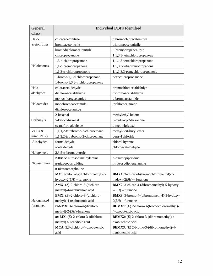
12

General Class

Individual DBPs Identified

chloroacetonitrile dibromochloracetonitrile bromoacetonitrile tribromoacetonitrile

Halo- acetonitriles

bromodichloroacetonitrile 3-bromopropanenitrile chloropropanone 1,1,3,3-tetrachloropropanone 1,3-dichloropropanone 1,1,1,3-tetrachloropropanone 1,1-dibromopropanone 1,1,3,3-tetrabromopropanone 1,1,3-trichloropropanone 1,1,1,3,3-pentachloropropanone 1-bromo-1,1-dichloropropanone hexachloropropanone

Haloketones

1-bromo-1,3,3-trichloropropanone chloracetaldehyde bromochloracetaldehdye Halo-

aldehydes dichloroacetaldehyde tribromoacetaldehyde monochloroacetamide dibromoacetamide monobromoacetamide trichloracetamide

Haloamides

dichloroacetamide 2-hexenal methylethyl ketone 5-keto-1-hexenal 6-hydroxy-2-hexanone

Carbonyls

cyanoformaldehyde dimethylglyoxal 1,1,1,2-tetrabromo-2-chloroethane methyl-tert-butyl ether VOCs &

misc. DBPs 1,1,2,2-tetrabromo-2-chloroethane benzyl chloride formaldehyde chloral hydrate Aldehydes acetaldehyde chloroacetaldehyde

Halopyrrole 2,3,5-tribromopyrrole NDMA: nitrosodimethylamine n-nitrosopiperidine n-nitrosopyrrolidine n-nitrosodiphenylamine

Nitrosamines

n-nitrosomorpholine MX: 3-chloro-4-(dichloromethyl)-5-hydoxy-2(5H) – furanone

BMX1: 3-chloro-4-(bromochloromethyl)-5-hydoxy-2(5H) – furanone

ZMX: (Z)-2-chloro-3-(dichloro-methyl)-4-oxobutenoic acid

BMX2: 3-chloro-4-(dibromomethyl)-5-hydoxy-2(5H) – furanone

EMX: (E)-2-chloro-3-(dichloro-methyl)-4-oxobutenoic acid

BMX3: 3-bromo-4-(dibromomethyl)-5-hydoxy-2(5H) – furanone

red-MX: 3-chloro-4-(dichloro methyl)-2-(5H)-furanone

BEMX1: (E) 2-chloro-3-(bromochloromethyl)-4-oxobutenoic acid

ox-MX: (E)-2-chloro-3-(dichloro methyl) butenedioic acid

BEMX2: (E) 2-chloro-3-(dibromomethyl)-4-oxobutenoic acid

Halogenated furanones

MCA: 2,3-dichloro-4-oxobutenoic acid

BEMX3: (E) 2-bromo-3-(dibromomethyl)-4-oxobutenoic acid

13

1.5 Public Health Risk Assessment and Risk Management 1.5.1 Overview Dealing with potential health risks from DBPs in drinking water involves both assessing and managing risks. There are countless definitions of the processes of risk assessment and risk management, but functionally for the purposes of this report they can be considered as:

Risk assessment is an organized, rational process used to evaluate available evidence to understand a problem and try to predict danger.

Risk management is a practical response to the identified problem that seeks to manage risks to tolerable levels.

Setting water quality guidelines for human health-based parameters is an exercise in risk management that should be informed by the process of risk assessment. This description itself will find some disagreement as a conventional view among regulators has held that the setting of guidelines or standards is done strictly by risk assessment, with the implementation of those guidelines or standards being considered risk management. There is no controversy about implementation of guidelines being risk management, where feasibility, economic and social considerations clearly play a major role. Disagreement may arise in recognizing that the process of setting a guideline number itself is an exercise in risk management because the final number that is adopted will reflect issues of feasibility, economic and social realities either implicitly or explicitly. For the specific case of the Guidelines for Canadian Drinking Water Quality, those considerations are explicit in the deliberations of the Federal / Provincial / Territorial Committee on Drinking Water, so there should be no debate that setting the guideline number (maximum acceptable concentration or MAC) is a product of both risk assessment and risk management. Risk assessment for these purposes can be seen to consist of 4 major steps:

1. Hazard Identification: identification of the nature of harm that may be caused to humans or experimental animals by the substance or circumstances being assessed; a critical element of this step should be a determination of the level of confidence in a causal relationship between exposure and adverse health effect

2. Exposure Assessment: evaluation of the degree of exposure that the human population will experience to the substance (i.e. water consumption, inhalation of volatile substances, dermal uptake from contact)

3. Dose – Response Assessment: estimation of the quantitative relationship between the degree of exposure (dose) and the level of harm that will arise

4. Risk Characterization: estimation of the level of risk for identified hazards by combining the estimated exposures with dose-response relationships

14

All of these steps involve complexity and uncertainty. Considerable progress has been achieved over the past few decades in monitoring and modeling for exposure assessment. However, to assess possible health risks from exposure to drinking water disinfection by-products, the most vexing problems continue to be determining how confident we can be about the existence of a relevant causal relationship and, if such a relationship is deemed sufficiently plausible, what dose-response relationship should be used to ultimately characterize the health risk to humans. Evaluating the evidence on causation is necessary to determine if there is a reasonable basis to believe that harm to human health could be caused by the substances in question. If causation is accepted, the nature of the dose – response relationship, combined with assessed levels of exposure and with prevailing risk management policies for the level of risk that is deemed tolerable, will determine the quantitative value for a MAC. 1.5.2 Hazard Identification and Weighing Evidence The primary sources of evidence for identifying hazards to health from various substances are basic physical / chemical properties, toxicologic evidence and epidemiologic evidence. The physical / chemical properties of a substance will bear on how it behaves in the environment and will contribute to routes of exposure and amenability to treatment. No further discussion of that aspect of hazard identification will be pursued in this document. Toxicologic and epidemiologic evidence are the main features that this report addresses, so these will be discussed below in more detail. 1.5.2.1 Causation and Weighing Toxicologic Evidence. The capability of a substance to cause harm to living organisms is assessed by the study of toxicology, which has evolved from the basic science of poisons (Klaassen 1996). This source describes toxicology as both an art and a science. Rigorous scientific method is required for the conduct and analysis of experiments, while interpretation of the results and applying them to assessing human risk requires substantial judgement that becomes an art. The underlying premise of all toxicology experimentation is that the dose of any substance will determine the severity of its toxic effects. Dose is determined by exposure conditions including the route (ingestion, inhalation, dermal uptake or injection) and the vehicle (the substance carrying the agent under study) which for our purposes will be drinking water for ingestion, air for inhalation or some other carrier for gavage (instillation by a tube into the alimentary canal). Dose should always be expressed in terms of the duration and frequency which can range from a short term, single dose for determination of acute responses, including lethality to continuous dosage over a lifetime for a chronic lifetime study, with multiple possibilities in between. The discussions that follow deal with lifetime (chronic) cancer studies and various studies on adverse reproductive outcomes (ranging from acute to subacute in relation to gestation). The dosing regimen is particularly critical to acquire meaningful biological evidence for the effects being studied (enHealth 2002). Because there are practical limitations on the

15

number of experimental animals that can be tested at any given dose level (a maximum of 50 animals is typically used at each dose level of lifetime cancer bioassays) resulting in costs in the millions of dollars, maximum doses tested will usually approach the maximum dose that the animals can tolerate for the duration of a lifetime experiment in order to maximize the chances of detecting an adverse response in a small population. Artifacts caused by high dose experiments do pose a concern for interpretation – “High doses that overwhelm normal mechanisms for metabolism, detoxification and/or excretion, or produce severe tissue damage (i.e. necrosis, demyelination) can make interpretation difficult or lead to inappropriate conclusions about the extent of the hazard.”(enHealth 2002). Criteria have been developed to assess what is appropriate for a maximum tolerated dose and includes ensuring that the dose does not: “Cause a body weight decrement from concurrent control values of greater than 10-12%; in a dietary study, exceed 5% of the total diet because of potential nutritional imbalances caused at higher levels, or; produce severe toxic, pharmacologic or physiological efects that might shorten duration of the study or otherwise compromise the study results; in a carcinogenecity study, alter survival in a significant manner due to effects other than tumour production” (enHealth 2002). Some of the factors considered in assessing the quality of experimental design include:

• adequacy of experimental design • appropriateness of observational and experimental methods • frequency and duration of exposure • appropriateness of species, strain, sex and age of animals • number of animals per dose group • justification of dose, route and frequency of dosing • conditions under which the substance was tested • use of good laboratory practice (GLP) • competency and completeness of study conduct and reporting • effects of modifying factors which may result in major inequalities between

control and test animals (many subtle, but important, factors may influence results) using historical data to judge consistency with past control experience

Some of the key factors that are normally evaluated in considering the weight of evidence from any particular toxicology study include:

• Judging which observed effects are truly toxic effects o Experimental testing is stressful and subject to interference (adaptation,

infection, etc.) o Animal dynamics can lead to biological responses

• Concurrent control groups are mandatory o Age matched o Sex matched o Strain matched o Animal selection must be randomized

• Use non-treated and vehicle-control groups

16

o Vehicle used to deliver agent is critical o Vehicle must be rationalized in relation to hazard being evaluated

• Animal handling o Controls must be handled identically with treatment groups o Both must get same level of attention from handlers

• Use historical data to judge what is normal Some specific concerns about the analysis of carcinogenicity bioassay data for quantitative cancer risk assessment are addressed in section 1.5.4 1.5.2.2 Causation and Weighing Epidemiologic Evidence. Ultimately, any initiative to assess risk to human health must carefully weigh any available evidence that addresses human health. Such evidence is gathered almost exclusively by epidemiologic methods studying human populations. Individual case reports of human illness are normally limited to situations involving high dose (e.g. poisoning incidents) or extremely rare outcomes with well established causal connections (e.g. chloracne from dioxin exposure). Case reports have no contribution to offer to the study of DBPs in drinking water. Epidemiology involves studies on human populations to determine any meaningful associations between exposure to hypothesized causal agents and adverse health outcomes (disease). This fundamental comparison of outcome in relation to exposure to a hypothetical cause requires that both outcome and exposure are known in as much detail and to the greatest degree of accuracy possible (at least in consistent relative terms) for every individual who will be studied. Epidemiology applied in search of causation is an exercise in determining the correspondence of the health outcome under study as it relates to an exposure that is the hypothetical cause of that outcome (e.g., to provide evidence that supports a hypothesis that smoking causes lung cancer it is necessary to show for a population that those who smoke end up suffering from lung cancer more than those who do not smoke). In its simplest terms, this may be seen as studying a 2x2 table where exposures and outcomes can be dichotomized as shown in Figure 1. Evidence of a positive association between exposure and disease arises when individuals in the study population are found more commonly in boxes a and d combined than in b and c combined.

Disease (+) No Disease (-) Exposed (+) a b

Not Exposed (-) c d Figure 1 Basic 2 x 2 Table for Epidemiologic Analysis Exposure to DBPs in drinking water is normally a continuous variable (dose determined by concentration in water and volume consumed), but this continuous variable is often dichotomized for analysis or is analyzed by logistic regression which accommodates

17

continuous data. In either case, the underlying premise of seeking an association between exposure and outcome is fundamental to the epidemiologic method. Because other factors will also influence health outcomes (age, sex, nutritional status, poverty, etc.), as many of these potential confounding factors must also be known in as much detail as possible to allow for an assessment of confounding. Confounding will arise from a failure to account in the analysis for exposure to a true causal factor. There is also a possibility in observational (vs. randomized experimental) studies for factors which may modify risk of the hypothesized outcome to be unevenly distributed among exposed and unexposed individuals. As well, most data collection will be imperfect and may be subject to bias, regardless of good intentions to find the truth. There are many sources of potential bias in the collection of epidemiologic evidence which can skew the results and either hide a true association or create a spurious association where one does not truly exist. Finally, regardless of how much care is taken in the gathering of evidence, random and sampling error is unavoidable. As a result, it is essential to always calculate a confidence interval for any estimate of an association between hypothetical cause and health outcome. Typically, the 95% confidence interval for a measure of association must exclude the null value (what would be measured if there was truly no association) to conclude that a finding is statistically significant. Generally, a wider confidence interval is indicative of a less stable association estimate. All else being equal, a study with a larger sample size will have greater capability of detecting a true association and thus should be accorded greater weighting in comparing results among various studies. There are several types of epidemiology study designs with varying complexity, rigor, cost and most important for this discussion, ability to test causality. A description of the different study designs is presented here to emphasize the importance of the study design to the ability of an epidemiologic study to test for causality, in relation to widely accepted criteria for causality. Of particular importance is that the study designs better at testing causality all use exposure and outcome data for individuals rather than for groups or populations. The utility of a study in testing a hypothesis of causality depends in part on whether individual exposure can be linked to individual outcome. The more accurately one can characterize the exposure and the outcome in each individual, the more useful a study will be in testing a hypothesis of causality. Generally, low cost, weaker study designs will be used to generate hypotheses of some environmental exposure causing a human health disease. Once clear hypotheses have been formulated, more complex analytical study designs are needed to test a hypotheis of causation. Epidemiology study designs can be described as experimental, or observational (Beaglehole et al. 1993). In experimental studies the investigator assigns the exposure levels and follows subjects for subsequent changes in health status.Types of experimental studies include randomized controlled trials (also called clinical trials), field trials, and community intervention and cluster randomized trials. Randomized control trials are rated the most

18

useful study design for testing causation. However, this type of study is rarely used in environmental epidemiology because of the ethical problems associated with experimentally exposing subjects to potentially harmful agents and the logistical demands that will be involved for studies that can meet ethics requirements. Observational studies fall under two categories of study design: analytical studies that investigate a relationship between health status and other variables, and descriptive studies that simply describe the health status of a community based on information already available, usually from public data bases. Descriptive studies do not compare health status in relation to other factors. There are several types of analytical study designs including cohort studies, case-control studies, cross-sectional studies, and aggregated studies. Aggregated studies have been referred to in the past as ecological studies but this label is distracting because these studies do not involve the science of "ecology". Aggregated studies use data from whole populations to compare disease patterns between different groups within a population during the same period of time or to compare disease patterns among the same group over several time periods. The units of observation are whole populations rather than individuals. Aggregated studies tend to be relatively quick and inexpensive to conduct as the information required is often already available from public records. Aggregated studies are often a first step in investigating a possible relationship between an exposure and a disease. However, there is a major disadvantage in aggregated studies that limits their usefulness. Because aggregated studies use data for a population rather than for individuals, exposure cannot be linked to disease in any particular individual. This can lead to a phenomenon called the "ecological fallacy" when inaccurate conclusions are made regarding relationships between exposures and outcomes based on aggregated data from populations rather than individuals. This error arises because population rate data do not allow any determination of whether the individuals who experienced an outcome were also exposed. Aggregated studies are only suitable to propose epidemiologic hypotheses, not to test them. Cross sectional studies, also called prevalence studies, measure disease state and exposure of individuals in a population simultaneously in time. This type of study provides a "snapshot" of the state of a population with respect to specific exposures and diseases at any one particular time. The major limiting factor of cross-sectional studies is that it is usually unclear whether exposure preceded, coincided with or followed the health outcome. This limits the capacity of cross-sectional studies to test causal hypotheses. In case control studies, subjects are selected based on whether they do (cases) or do not (controls) have the health outcome in question. The groups are then compared with respect to the proportion of each group with the exposure or characteristic of interest. Case control studies are relatively inexpensive and take less time to complete relative to cohort studies. They offer a solution to the difficulties of studying health outcomes with long latency periods, and they allow an investigation of many etiologic exposures or characteristics for a specific health outcome. However, case control studies are only

19

practical for relatively common diseases because of the need to assemble an adequate number of cases for analysis. Both the exposure and the disease must have occurred at the start of the study. This fact makes case control studies subject to possible bias on exposure status for the selection of cases vs. selection of controls (selection bias), or differential reporting of past exposure data based on disease status (recall bias). In the latter circumstances, those with a disease (cases) are usually more likely to recall exposures to hypothetical causes than those who are free of the disease (controls). Exposures may be determined from public or employment records or by interview with cases and controls, or by designated responders (e.g. a relative) where participants are deceased. Case control studies may be the only feasible approach for rare diseases or those with long latency periods. Although they are subject to a lot of serious challenges to avoid bias, they are moderately useful for testing causal hypotheses. With cohort studies, a group without the disease under study is selected and followed over time with their exposure status (exposed or not exposed) determined as they are followed. Subjects are then compared based on the proportions of exposed vs. non-exposed individuals who develop the outcome of interest subsequent to the exposure. Cohort studies can be retrospective or prospective. In retrospective studies all exposures and outcomes have occurred at the initiation of the study. Exposure status is determined from a time before the outcomes occurred. In prospective studies, the exposure may or may not have occurred at the initiation of the study, but the outcomes have certainly not occurred. The exposed and non-exposed subjects are then followed for occurrence of the health outcomes of interest. Because study subjects are free from the disease at the time of initiation of the study, the temporal sequence between the exposure and the outcome can be established. In addition, because the study groups are selected based on exposure status, cohort studies are ideal for studying rare exposures or for studying multiple outcomes from the same exposure. However, cohort studies are very time-consuming and expensive. As subjects must be followed for many years after exposure, there is the potential for bias caused by differential loss of subjects to follow-up. Cohort studies are not practical for very rare diseases because the size of the cohort necessary to generate sufficient cases for analysis may not be feasible. The “gold standard” in epidemiology with regard to generating evidence on causality is the experimental design typically used in clinical trials of drugs or medical interventions. In these designs, individuals are recruited and randomly assigned to control or treatment (exposed) groups. Randomization of assignment to treatment or control group can substantially reduce but cannot completely eliminate the chances of bias. Likewise, blinding of both participants and researchers (double-blinding) to the exposure status of the individual for the measurement of outcomes is also designed to reduce sources of bias. The experimental design may allow for a cross-over, whereby those who were unexposed are switched to the exposed category and vice-versa, to further reduce the potential impacts of undetected bias. These studies are very complex, time-consuming and expensive. They cannot be used for rare outcomes or for outcomes with long latency periods. Finally, the experimental design must contemplate an intervention that reduces otherwise “normal” exposure, rather then adding an environmental exposure, in order to qualify for ethics approval. Unlike medical research, where ethical assessment can

20

consider potential benefit to the individual to balance whatever risks may be imposed, environmental health research is not likely to benefit any individual participant sufficiently to warrant imposing a risky exposure. The implications of study design to the assessment of evidence for causality are discussed below. Criteria of causality have been derived from a set of concepts set out by Sir Austin Bradford Hill (1965) and by the U.S. Surgeon General (U.S.PHS 1964). They have been adjusted over the years by many commentators, but the original concepts remain sound. This review draws upon the excellent and accessible introduction to epidemiology by Beaglehole et al. (1993). They refer to seven criteria: temporal relationship, plausibility, consistency, dose-response relationship, strength of associaton, study design and reversibility.We will deal with the first six because reversibility is limited to outcomes that are reversible, something that does not apply to the outcomes generally being assessed for causation by chlorination DBPs. 1. Temporal relationship. Simply stated, the cause must precede the effect. If the cause does not precede the effect, then there are no grounds upon which to base causality. This criterion demands an accurate reckoning of the time relationship between the proposed exposure and the resulting outcome and as such requires a certain level of accuracy in the determination of both the exposure and the outcome. Because of the importance of this temporal relationship, the most powerful epidemiology studies will be based on incident (new) disease, rather than existing or prevalent disease, because the timing of disease onset can be known, thereby allowing for an assessment of whether the exposure has predated the outcome. 2. Plausibility. We must ask: is it biologically plausible that the exposure will cause the hypothesized outcome? This question is best answered by toxicology studies or in the absence of specific toxicology results, an assessment must be made of how reasonable it is to presume that agent X can cause outcome Y. An exposure-outcome relationship with a biologically plausible mechanism from toxicology studies provides a strong argument in favour of causality. If a biologically plausible mechanism is not obvious, the argument for causality is not disproven. Biological plausibility is often dependent on the state of the science at the time of investigation. If biological plausibility is not evident at the time of the investigation of the causal relationship, it may become apparent from future research. 3. Consistency. If several different studies with a variety of designs, carried out in different locations and under truly different conditions, consistently report the same result then the argument for causality is strengthened. However, a lack of consistency does not necessarily preclude a causal association. The differing study designs and circumstances (such as exposure levels) could reduce the impact of the causal agent in some of the studies. Therefore the studies with the best designs must be assigned the greatest weight when evaluating this criterion.

21

4. Dose-response relationship. A dose-response relationship has been demonstrated if the frequency or severity of the outcome increases with increasing frequency or magnitude of exposure to the potential causal agent. A clear dose-response relationship can be a good indication of a causal relationship, provided care is taken to assure that no un-recognized confounding or bias could be the underlying reason for the relationship. For those exposures and effects for which a dose-response relationship is valid, defining that dose-response relationship depends on defining both the dose and the response accurately. It follows that to have confidence in a dose-response relationship, there must be accuracy in the identification and quantitation of the exposure, as well as in the determination of the outcome. 5. Strength of the association is measured by the rate ratio (commonly called relative risk, RR) or the odds ratio (OR is an estimate of RR that is generated by case control studies) for a particular exposure – outcome comparison. The Odds Ratio compares the occurrence of exposure in the cases and the controls, with

controlsin exposure of Odds

casesin exposure of OddsOR =

OR = 1.0 is the null value, no association between exposure and outcome OR > 1.0 suggests that exposure is positively associated with disease (i.e.

exposure is more common in cases than in controls) OR < 1.0 suggests that exposure is negatively associated with disease (i.e.

exposure is less common in cases than in controls)

The Risk Ratio (Rate Ratio or Relative Risk) compares the rates of incidence of disease in exposed and unexposed groups as a ratio

group unexposedin rate Incidence

group exposedin rate IncidenceRR =

RR = 1.0 is the null value, no association between exposure and outcome RR > 1.0 suggests that exposure is positively associated with disease (i.e.

incidence of the outcome is greater in the exposed than in the unexposed group)

RR < 1.0 suggests that exposure is negatively associated with disease (i.e. incidence in the exposed group is less than in the unexposed group)

The RR is preferred as a measure of association over OR, but it is not possible to directly determine the RR in a case-control study because the incidence rates are not known directly because the study starts with an intentional sample of cases. The less common a disease is (more rare), the closer the estimate of OR will converge on the RR. For the purposes of this evaluation where most of the disease outcomes being studied are not common, the OR becomes a reasonable estimate of RR. A large RR argues more strongly

22

for causality than does a small one. However, a small RR does not preclude a causal association since the size of the RR can depend on the prevalence of other possible causes in relation to the agent of interest. In this fourth criterion, the necessity of accurate individual exposure assessment is emphasized. It is generally accepted that if an association is causal, weak exposure assessment resulting in non-differential misclassification of exposure will bias the resulting RR towards the null value, showing a weaker association than truly exists. The logic follows, therefore, that if an association is causal, more accurate exposure assessment should increase the apparent strength of the association. There is always the possibility that a weak association really is an indication of a non-causal association. In this case, all efforts must be made to develop a strong study design with adequate statistical power using accurate exposure assessment to ensure a study with minimal bias so that the conclusion of a non-causal association can be made with some confidence. Exposure assessment is universally acknowledged as a weakness in environmental epidemiology studies. Weak exposure assessment will inevitably result in misclassification of exposures which will cause the OR or RR that is calculated to be inaccurate. Considerable advances have been made in characterizing human exposure to DBPs so that total exposure is now understood to include activities such as showering, bathing and swimming (particularly for volatile DBPs) rather than simply ingestion. This subject is discussed further in the next section. Epidemiologists often rely on the statistical reality that non-differential misclassification of exposures will have the effect of attenuating the resulting OR or RR. This means that poor exposure assessment can be acknowledged while relying on an expectation that improved exposure assessment will inevitably result in an increased OR or RR. Of course such improvement will only happen if the cause under study is a true cause. This opens the prospect of pursuing improved exposure assessment for attempts at replicating or refuting earlier findings. This has been done in the case of investigating a possible association between spontaneous abortion and exposure to THMs (Savitz et al. 2005; Waller et al. 1998) that is discussed in Section 3.2.1. 6. Study design. As noted above, there are many different epidemiologic study designs, each with a different level of ability to test for causation. The best study design for testing causation is the randomized controlled trial or clinical trial. This type of study is rarely done in environmental epidemiology because of the ethical limits on experimentation with humans. Notable exceptions relevant to drinking water have been the randomized intervention trials performed in Melbourne, Australia and in Iowa, U.S.A. to investigate the risk of gastrointestinal disease from drinking water exposure (Hellard et al. 2001; Colford et al. 2006, 2005). Prospective cohort and case-control studies are the next-best study designs and these are commonly used in environmental epidemiology. Retrospective cohort and cross-sectional studies are less able to test causation. A retrospective cohort often suffers from limited to non-existent individually-validated exposure information and current cross-sectional studies will not provide evidence of a

23

temporal relationship (the cause must precede the effect) The strengths and weaknesses of these study designs is discussed in more detail below. 7. Reversibility. This criterion means that if a potential causal agent is removed, the probability of the outcome should decrease. If the removal of a potential causal agent results in a decrease in the occurrence of the outcome, then the argument for a causal relationship is strengthened. It is necessary in evaluating this criterion that an accurate assessment of exposure or non-exposure to the potential causal agent be determined. It is important to note that this criterion is limited to causal processes that involve reversible mechanisms. The cross-over incorporated into the randomized double-blind drinking water study addressing gastrointestinal illness from well-treated drinking water in Iowa (Colford et al. 2005) may be considered a version of reversibility. Even with these criteria, there is no absolute rule for judging a potential causal relationship. All available evidence must be considered when determining whether an exposure really is the cause of an outcome. In the case of conflicting evidence, the types of evidence must be weighed with respect to their relative positions within the criteria for causality. Most importantly, a temporal relationship between the cause and the effect must be established. If the effect precedes the alleged cause, then there is no argument for a causal relationship. Plausibility, consistency, and dose-response are all very important criteria. The likelihood of a causal association is increased if evidence representing several of the criteria all points to the same conclusion, i.e consistency. The strength of association must be judged by how far-removed from the null value the estimate of RR is, but also the size of confidence interval and the exclusion of RR = 1.0 are important. 1.5.3 Assessing Exposure Compared to the challenges of assessing toxicity, the assessment of exposure to DBPs seems a substantially less daunting task, particularly if we imagine that the only route of exposure for humans to substances in drinking water is via ingestion. However, because humans use tapwater for showering, bathing and a variety of household uses, it is not accurate to assume that direct ingestion is the only important route of exposure to DBPs (Figure 2). In fact, studies with volatile DBPs like THMs have shown that exposure via showering and bathing can be substantial in relation to direct ingestion (Arbuckle et al. 2002, Backer et al. 2000, Jo et al. 1990). These factors, combined with the higher levels of DBPs commonly found in swimming pools, have raised the matter of swimming as an additional risk factor for DBP exposure. Among the individual issues that may arise from these additional realities are individuals (who may be pregnant) such as institutional caregivers who have to supervise client bathing as a regular activity. The problem of exposure assessment becomes even greater when individual exposure assessment is required for epidemiology studies (Arbuckle et al. 2002). In fact, the difficulty of accurately assessing exposure provides a major shortcoming of epidemiology studies addressing chlorination DBPs in drinking water.

24

Figure 2 Exposure Pathways for Chemicals in Tapwater (after Olin 1999) Challenges of exposure assessment include: (1) limited information on the identity, occurrence, and toxicity of the many DBPs that can be formed by disinfection; (2) the complex, time variable chemical relationships affecting DBP concentrations within a municipal water distribution system; and (3) practical difficulties in acquiring accurate and reliable information on personal activity determining exposure from non-ingestion pathways as well as water consumption rates. One approach that has been suggested as a possible gold standard for DBP exposure assessment would be a biomarker (Swan and Waller 1998). The volatile DBPs like chloroform are metabolized far too rapidly and they can be detected in human blood for only minutes after a shower exposure, but not at all after ingestion exposure because they are metabolized so rapidly. Ingestion and uptake from the gastrointestinal tract leads directly to the liver where metabolism eliminates them from the bloodstream, compared with inhalation which allows them to reach the bloodstream directly, where they can be measured until the biomarker has been circulated through the liver. Some success has been achieved in demonstrating trichloroacetic acid as a possible biomarker of drinking water exposure because it is metabolized relatively slowly (Kim et al. 1999, Froese et al. 2002). The half-life of trichloroacetic acid following drinking water ingestion has been found to range from 2.1 to 6.3 days (Bader et al. 2004).

CONTACT PATHWAYS: Chemical-specific

Direct/indirect Volatile/nonvolatile

Aerosol

Dermal (skin) Ingestion

(gastro – intestinal tract)

Respiratory (lung)

Vapour Water

Water source characteristics

Building characteristics

Activity Patterns

Demographics

Activity Data

Morbidity and Mortality Data

M M M

Systemic Circulation

Liver Metabolism -

first pass effect

Distribution to Target Organs

ABSORBED DOSE

ROUTE OF ENTRY (PENETRATION)

EMISSION & TRANSPORT

M = metabolism at tissue of contact

25

1.5.4 Quantifying Risk (Estimating Dose – Response Relationships) Historically, risk assessment involved a clear distinction between how carcinogens and non-carcinogens were treated. Typically, this distinction involved identifying a no observed adverse effect level (NOAEL) from a dose-response curve for non-carcinogens which were assumed to exhibit a threshold dose below which no toxic response would be expected. In instances where an adverse effect was observed even at the lowest does tested, a lowest observed effect level (LOAEL) value may be used instead, with appropriate adjustment in the uncertainty factors (UF). A set of UF were then applied to the NOAEL or LOAEL to develop a reference dose (RfD), also referred to as a tolerable daily intake (TDI).

[UFn]...[UF2][UF1]LOAELor NOAELTDIor RfD

•••=

UF are used to account for a number of uncertainties in extrapolating an animal toxicology result to a human risk assessment. Included among the factors that could be accounted for were:

• animal to human extrapolation accounts for variation between experimental animals and humans (typically 10)

• human heterogeneity to account for variation of sensitivity within the human population (typically 10)

• subchronic to chronic extrapolation accounts for the possible difference between a NOAEL derived from less than lifetime study and a lifetime study (typically 3, up to 10)

• LOAEL to NOAEL accounts for having to rely upon a LOAEL if a NOAEL has not been measured (up to 10)

• adequacy of database accounts for judgements about the uncertainty associated with having to rely upon incomplete data (up to 10)

• modifying factor to assess the quality of data available (up to 10) If all of the above were applied simultaneously, the combined product of UF would be 1 million leading to a reduction of a LOAEL from a less than life-time study by 1 million fold. Such an application would be an admission that we know virtually nothing about the substance, so the practice had been to limit the combined UF to no more than 10,000 (USEPA 2004). Even this level of uncertainty was unsatisfactory, so current practice is to limit the combined uncertainty factors to 3000 or less if this approach was to be used for setting a regulatory number. The location of a NOAEL and a LOAEL for a hypothetical dose-response curve is shown in Figure 3. A substantial improvement on the NOAEL / LOAEL approach is the so-called benchmark dose (Crump 1995), which applies statistical modeling of the experimental dose – response curve to set an estimate of a dose for a specified response level (5 or 10%) that is then used to define the resulting RfD.

26

Figure 3 NOAEL and LOAEL on a dose – response curve (adapted from Paustenbach

1989) In contrast, carcinogens were assumed, by default, to have no threshold such that the dose-response curve obtained from a cancer bioassay was extrapolated to zero dose, corresponding to zero excess risk of cancer (above background). The commonly used default model was the so-called “linearized multi-stage” (LMS) model which used an exponential expansion equation to fit the bioassay data points (normally only 2 or 3 doses in a cancer bioassay). The equation for the LMS model was: where P is the probability of cancer at dose = d At a very low dose, d is very small, making d to higher powers insignificant in this additive equation, so that the excess risk (ER) calculated by this equation at very low dose (d), simplified to:

[ ])dqdq(qexp1P kk10 +++−−= L

Risk

Dose

below experimental detectionmodel extrapolation required

detectable by experiment

NOAELLOAEL

Risk

Dose

below experimental detectionmodel extrapolation required

detectable by experiment

NOAELLOAEL

27

ER(d) = q1* d This means that the cancer risk at low dose is calculated by a simple linear equation with a cancer slope factor (CSF) = q1* for the LMS times the dose. The *designation in this case means that the slope is actually determined as the upper 95% confidence interval on the estimated slope. This low dose risk extrapolation approach means that the estimated CSF is the determining number derived from modeling a cancer bioassay. It is predicated on the assumption that the low dose model travels linearly through the origin. That assumption is a science policy decision that is derived from the possibility that a single molecule of a genotoxic (DNA-damaging) carcinogen could damage the DNA of a single cell in exactly the right manner that if that cell survived to replicate, the damaged DNA (mutation) could be replicated in daughter cells that could reproduce exponentially to ultimately develop into a tumor. A remarkably insightful finding about the meaning of the CSF estimated in this manner from cancer bioassays based on the maximum tolerated dose and only one or two other doses at a fixed fraction of the MTD (typically MTD/2 and possibly MTD/4) is illustrated in Figure 4.

Figure 4 Association Between Cancer Slope Factors and Maximum Tolerated Dose

(MTD) Used in Rodent Carcinogen Bioassays (Krewski et al. 1993)

28

Figure 4 depicts the results from what were independent experiments each on a different chemical, but all using the same protocol based on MTD being the maximum dose tested. The figure shows that individual chemical MTD values ranged over 10,000,000,000 fold, as did the calculated CSF. Yet, this large number of experiments over a huge range of toxicities yielded a correlation coefficient of -0.941, an inconceivably high value if these rodent bioassay experiments were truly independent. An inescapable conclusion arising out of the results presented in Figure 4 is that a primary determinant of the CSF for any of these chemicals was its MTD. Looking more closely at Figure 4, the scatter about the fitted regression line is contained in a 95% prediction interval that ranges over a little more than 2 decades (100 fold). In any of these cancer bioassays, with 50 animals per dose level, the maximum measurable range of response would be 2% to 100% (1 out of 50 up to 50 out of 50 animals developing cancer) which suggests that all of the information on carcinogenic response obtained from each bioassay is depicted in the vertical scatter within the prediction interval of Figure 4. However, the apparent effect of MTD in determining the CSF is much larger. Because it is extremely unlikely that such results could be obtained for truly independent experiments, there must be an explanation for what is shown in Figure 4 and it is provided in Figure 5. Figure 5 Explanation of Remarkably Strong Association Between CSF and MTD

(Hrudey 1995)

CSF, cancer slope factor

bioassay dose range set by the maximum tolerated dose, MTD, which is governed by the systemic toxicity of the chemical and found to range over 9 orders of magnitude for the range of chemicals tested in cancer bioassays

bioassay response range is governed by the number of test animals used, typically 50, which in turn limits the measured response range to only 2 orders of magnitude, from 2% to 100%

the dose-response line is anchored at (0,0) and the resulting linear slope is determined by the lowest measured response and dose values

CSF, cancer slope factor

bioassay dose range set by the maximum tolerated dose, MTD, which is governed by the systemic toxicity of the chemical and found to range over 9 orders of magnitude for the range of chemicals tested in cancer bioassays

bioassay response range is governed by the number of test animals used, typically 50, which in turn limits the measured response range to only 2 orders of magnitude, from 2% to 100%

the dose-response line is anchored at (0,0) and the resulting linear slope is determined by the lowest measured response and dose values

29

This shows that the policy assumption which anchors the linear low dose slope at the origin of the dose response curve combines with the point of departure for the linear, low dose modeling to determine the CSF. A chemical which has a very low acute toxicity, i.e. also be very large values on the log scale shown in Figure 4, so that the low dose slope, anchored at the origin and extrapolated down from a point of departure far to the right of Figure 5, will inevitably correspond to a shallow CSF. On the other hand, a chemical which has very high acute toxicity, i.e. a very low MTD, will have its point of departure much closer to the origin, thereby yielding a very steep CSF. The result of this analysis is that the critical factor derived from the cancer bioassay for calculating cancer risk, the CSF, is determined by the method that is driven by a combination of the policy assumption to anchor the slope at the origin and to use MTD and high fixed fractional doses thereof as the point of departure for the linear model. This reality means that the predicted cancer risk is at best an upper bound estimate of the worst that the cancer risk could be. That realization combined with the intended use of an upper 95% confidence interval prediction for the CSF largely assures that any prediction of cancer risk with this methodology is extremely unlikely to underestimate the cancer risk. Such a prediction is certainly not an estimation of expected cancer risk. The 1986 U.S. EPA guidelines for carcinogen risk assessment explicitly stated about the CSF (it was called a cancer potency factor at that time): “It should be emphasized that the linearized multistage procedure leads to a plausible upper limit to the risk that is consistent with some proposed mechanisms of carcinogenesis. Such an estimate, however does not necessarily give a realistic prediction of the risk. The true value of the risk is unknown, and may be as low as zero.” Although this clear statement was not included in subsequent cancer risk assessment guidelines, its validity was acknowledged in a more recent examination of U.S. EPA risk assessment procedures (USEPA 2004). In addition to the caution that is necessary in viewing the quantitative cancer risk estimates that have been commonly derived from the use of the CSF approach, the current cancer risk assessment guidelines USEPA 2005, first proposed in 1996, have acknowledged that not all chemicals that produce a carcinogenic response in a cancer bioassay do so by a genotoxic (DNA-damaging) mechanism. This is a vitally important distinction because the key assumption underlying the linear extrapolation of the low dose model to the origin of the dose response curve is that DNA damage can be caused, which can subsequently (at least in theory) be reproduced by cell replication to ultimately yield a tumor. If a substance produces excess tumors in the exposed animals by some mechanism other than DNA-damage, it is not appropriate to assume that there is no threshold and invoke the low dose linear extrapolation to estimate a CSF for risk assessment. The most common example of a mechanism that is not genotoxic is cytotoxicity, i.e. the killing of cells, which can lead to an organ response of cell proliferation to replace the killed cells. This proliferation response creates an increased chance of naturally-occurring DNA replication errors, some of which may lead to tumors. However, the cytoxicity will normally exhibit a threshold and will not cause a cancer risk

30

below that threshold. As discussed later in Section 2.1.1, this was demonstrated in the case of chloroform administered at high bolus doses in corn oil by gavage (NCI 1976). 1.5.5 Characterizing Risk Once the hazard has been identified and evaluated (cancer risk, reproductive risk, etc), expected exposure levels have been characterized and estimated, dose-response relationships have been derived, most commonly from toxicology experiments, the risk can be characterized. For threshold chemicals, an expected exposure scenario can be assessed by taking a ratio of the expected exposure dose over the RfD or TDI. This ratio has been assigned a variety of names including a hazard quotient or a margin of exposure. If that ratio is substantially greater than 1.0, then the predicted exposure scenario will cause an exposure that exceeds the TDI and measures should normally be pursued to reduce exposure in such cases. Because of the application of substantial uncertainty factors onto a NOAEL that is normally used for setting a TDI, toxic effects would not be expected if the ratio is within a few multiples of 1.0 (say less than 10). If this approach is used for setting a MAC, the exposure concentration is calculated according to what it would have to be to yield the TDI. That concentration then becomes the MAC.

CRSABWTDIMAC ••

=

where:

MAC is the maximum acceptable concentration in water (µg/L) TDI is the tolerable daily intake (µg/kg-bw d) BW is the human body mass (kg-bw) SA is a source allocation that estimates what portion of total daily exposure

comes from drinking water (dimensionless), often assigned as 20% in the absence of knowledge about other sources of the chemical being assessed

CR is the contact rate in equivalent tapwater ingested (L/d) For non-threshold chemicals where a CSF has been estimated from a long term cancer bioassay, it is commonly adjusted for humans from rodents by a body mass scaling factor:

body mass scaling factor = (rodent body mass / human body mass)1/4 The adjusted CSF can be used to calculate a risk-specific dose by rearranging the low dose extrapolation equation:

ER(d) = CSF RSD

31

to:

RSD = ER(d) / CSF

where:

RSD is the risk specific dose (µg/kg-bw d) CSF is the cancer slope factor (µg/kg-bw d)-1 ER(d) is the target lifetime cancer risk, typically 10-5 in Canada (dimensionless)

Then the MAC can be calculated as:

CRSABWRSDMAC ••

=

where:

MAC is the maximum acceptable concentration in water (µg/L) RSD is the risk specific dose for 10-5 lifetime cancer risk (µg/kg-bw d) BW is the human body mass (kg-bw) SA is a source allocation that estimates what portion of total daily exposure

comes from drinking water (dimensionless) often assigned as 20% in the absence of knowledge about other sources of the chemical being assessed

CR is the contact rate in equivalent tapwater ingested (L/d) 1.5.6 Decision-Making and Implementation of Risk Management Some key concepts for assessing evidence have an important bearing on decision-making under uncertainty. These are: standard of proof, burden of proof, types of decision error (false positive or type 1 error, false negative or type 2 error, and incorrect problem or type 3 error). The standard of proof is a statement of how confident we must be that the evidence truly shows us what we ultimately judge it to show us. In our legal system criminal prosecutions require proof beyond a reasonable doubt for a conviction. This is a very high standard of proof which reflects a societal position that we would far rather allow a guilty person to go free than to wrongfully convict an innocent person. There is no clear quantitative statement that accurately captures this level of confidence, but it is obvious that beyond a reasonable doubt is intended to allow for only a very small (but non-zero) probability of convicting an innocent person. A much lower standard of proof is used in civil litigation where decisions are made on a balance of probabilities. This means a finding that something is more likely than not (i.e. 51 to 49% probability) is sufficient to make the judgement.

32

The burden of proof deals with the issue of who holds the responsibility for proving the case. In criminal law, the prosecution bears the burden of proof and in civil law, the complainant bears the burden of proof. Deciding who must bear the burden of proof is critical to any decision-making process because the party who must discharge this burden is the party who is saddled with resolving the inevitable uncertainty that will arise in any interpretation of evidence. While the matters of standard and burden of proof are explicitly defined in our legal system, these matters are generally not explicitly defined in our environmental health regulatory system. The movement advocating the precautionary principle for environmental regulation provides examples of reversing the onus on regulators to prove harm for a given substance versus placing the onus (the burden of proof) on the producer of a substance. In providing for a reverse onus there is an inevitable problem of asymmetry of the concepts that need to be proven. This also involves an interaction between the burden and the standard of proof. Referring back to the legal system, we can require the prosecution to prove guilt beyond a reasonable doubt, but it is not realistic to require the accused to prove innocence beyond a reasonable doubt. This asymmetry arises because there may be a fuzzy transition from guilt to innocence. In absolute terms, if innocence means the absolute absence of any guilt, proving innocence requires proving a negative, something that our evidentiary logic system finds difficult. Put in terms of environmental health issues, it may be possible to prove (to some specified standard of proof) that a substance poses a specific danger. However, simply reversing the onus to require producer of a substance to prove a substance poses “no danger” raises an essentially open-ended range of possibilities that amounts to proving a negative. In the case of drinking water quality, there has not been a clear articulation of who bears the burden of proof, nor what standard of proof is required. The reality has been that regulators will identify substances that may pose a health risk to consumers and will set about gathering evidence to prove the case. Drinking water providers may be consulted about practical realities that may arise from implementing a MAC for a particular substance, but they have certainly not been charged with the burden of proving that a given substances poses no danger. The only cases where drinking water providers have generally been assigned a burden of proof arises in cases where they wish to be exempted from a regulated requirement (i.e. filtration of surface water supplies) or wish to substitute a treatment process for what is deemed to be conventional practices (i.e. substituting UV disinfection for chlorination). While regulators have generally accepted the burden of proof for establishing the need for a MAC for any particular substance in drinking water, they have clearly not accepted (nor should they) a standard of proof of beyond a reasonable doubt. What standard of proof is required has not been articulated. It may be that proof on a balance of probabilities has been the intended, but unstated, target but a case can be made that, having accepted the burden of proof, which might more logically reside with provider of the service, regulators have taken a public health stance leaning towards a more

33

precautionary position on the standard of proof. In other words, adopting a MAC for a substance does not demand that the causal link is more likely than not, rather the MAC may be adopted on the basis of there being a reasonable possibility that the substance in question will cause harm via drinking water exposure. Decision errors can arise any time we attempt to use evidence to justify a decision (Hrudey and Leiss 2003). A false positive error is one where we decided to act when, in reality, the action was not justified. In public health terms this might be a case where a boil water advisory is called on the basis of a monitoring mistake. A false negative error is a case where no action is taken on the basis of the evidence, but in reality, action should have been taken. The type 1 and type 2 designations arise from statistical hypothesis testing. The third type of error, wrong problem error, is where a decision is taken on evidence that does not apply to the problem that is being dealt with (Kendall 1957). In this case, a type 3 error, the evidence is irrelevant to the decision. In terms of drinking water contaminant MAC values, a type 1 (false positive) error would be a decision to develop a MAC when the reality is that one is not required. A type 2 (false negative) error would be a decision to not develop a MAC when one is required. A type 3 (wrong problem) error would be a decision to develop a MAC when some other measure (i.e. a practice guideline) is required. There are negative consequences possible for any one of these decision errors. The negative consequences and their severity are obviously situation-specific, but it should be clear that a precautionary stance to avoid false negative errors at any cost will inevitably cause an unacceptably high rate of false positive errors (Hrudey & Leiss 2003). Likewise, accepting that any action is better than none may give rise to avoidable type 3 errors where resources are dedicated to a problem that they fail to solve, leaving any resource-constrained system vulnerable to other potential failures.

34

2. CHLORINATION DISINFECTION BY-PRODUCTS AND CANCER 2.1 Toxicology Evidence from Long Term Studies on Cancer A historical overview of the risk assessment and regulation of chloroform was given in section 1.3. The discussion that follows considers the available evidence from long-term (near lifetime exposure) cancer bioassays in more detail to provide some background to that previous historical account. 2.1.1 Chloroform Chloroform is the main component of trihalomethanes. It has a long history in relation to human health. It was adopted in the mid-1800s as an anaesthetic. Ironically chloroform as an anaesthetic provided John Snow with the livelihood to support his research interests which allowed this pioneering medical scientist to establish the link between fecal contamination of drinking water and cholera by applying epidemiologic investigation to cholera outbreaks (Vinten-Johansen et al. 2003). Choroform was used until the 1970s in a variety of consumer products ranging from mouthwash to toothpaste. Long-term experimental studies on chloroform to detect carcinogenicity are summarized in Table A1-1 (Appendix 1). Chloroform was tested in mice and rats in a cancer bioassay (NCI 1976). These studies were designed to determine the potential for chemical substances to cause cancer in mammals and they were designed to maximize the ability of the experiment to reveal any carcinogenic effect. Dosing in this experiment was done as a daily bolus dose of chloroform dissolved in corn oil. The initial high dose in female rats of 250 mg/kg-d had to be reduced to 180 mg/kg-d after 22 weeks because of frank toxic effects. Mice proved more tolerant to chloroform so that their initial doses of 200 and 400 mg/kg-d were increased after 18 weeks to 300 and 500 mg/kg-d. The results of this high dosing showed strong evidence of liver tumors in mice (98% of males and 95% of females at lifetime average doses of 277 mg/kg-d and 477 mg/kg-d, respectively; 36% of males and 80% of females at lifetime average doses of 138 and 238 mg/kg-d respectively) in the mouse experiments. The high dose levels were from 27 to 115% of published median lethal doses for mouse (Hill et al. 1975), suggesting that the B6C3F1 mouse was unusually tolerant to the acute toxicity of chloroform. In contrast, the rats dosed at up to 200 mg/kg-d failed to show excess liver tumors relative to controls. A series of bioassays with various strains of mice at doses up to 60 mg/kg-d (by gavage in toothpaste) failed to show liver tumors in excess of control (Roe et al. 1979). Even more relevant for evaluating drinking water risk was a bioassay done with female B6C3F1 mice that used chloroform in drinking water at doses up to 263 mg/kg-d (water concentration of 1800 mg/L) which found no excess liver tumors relative to controls. Other bioassays using gavage of chloroform in toothpaste with rats (Palmer et al. 1979) and beagle dogs (Heywood et al. 1979) did not find any evidence of excess liver tumors. The evidence of the early rodent bioassay (NCI 1976) was negative for kidney tumors in mice but showed elevated kidney tumors in rats at the 90 mg/kg-d and 180 mg/kg-d dose

35

levels. Palmer et al. (1979) found no evidence of kidney tumors in rats at 60 mg/kg-d and Heywood et al. (1979) found no evidence of kidney tumors in beagle dogs at 30 mg/kg-d, but Roe et al. (1979) found excess kidney tumors in mice at 60 mg/kg-d. An oral dosing experiment in drinking water (Jorgenson et al. 1985) found increasing kidney tumor incidence with increasing dose level above 200 mg/L relative to the control, but only 1800 mg/L was significantly elevated in relation to the control. Hard et al. (2000) performed a re-evaluation of the Jorgenson et al. (1985) rat bioassay results and found that all the rats at 1800 mg/L and half of those at 900 mg/L chloroform exposure showed evidence of cytotoxicity and regenerative cell proliferation. A few key insights can be drawn from the relatively extensive long-term animal testing of chloroform for carcinogenicity. The dosing method and vehicle are clearly important. The initial extremely high dose bioassays showing a dramatic liver tumor response in mice and a significant kidney tumor response in rats (NCI 1976) was obtained where dosing was done by a daily bolus of the high chloroform dose dissolved in corn oil. The effects of this dosing regime involved a vehicle (corn oil) that would facilitate rapid uptake from the gut and the single bolus dose mechanism would deliver the chloroform rapidly at a very high concentration. In contrast, providing high concentrations of chloroform dissolved in drinking water (Jorgenson et al. 1985) allowed the animals to take their dose spread out somewhat over the day in a vehicle that does not necessarily enhance the uptake of chloroform from the gut as corn oil does. The net effect is that the liver, which is the first organ that the chloroform will encounter upon entering the blood stream after crossing from the gastrointestinal tract will see much higher spikes of chloroform concentration with corn oil gavage than with drinking water ingestion, for the same nominal daily dose. The resulting impact of extremely high doses of chloroform to the liver was first noted as evidence of cytotoxicity on liver cells. The potential carcinogenic consequence of killing liver cells is that liver tissue will regenerate and the more regeneration that must be provided by the organism seeking to cope with the repeated and massive loss of liver cells is that regenerative proliferation of cells can be expected to increase the risk of cell replication errors, thereby increasing the likelihood of genetic mistakes (mutations) giving rise to tumor initiation. This is a distinctly different mechanism of carcinogenesis than a genotoxic effect of the carcinogen directly on a cell whereby chemically induced damage to DNA of that cell can cause mutations that give rise to tumor initiation. This distinction in mechanism justifies a threshold approach to risk assessment rather than a no-threshold approach predicated on a genotoxic mechanism. Support for the action of chloroform by a cytotoxic rather than a genotoxic mechanism was very clearly provided by additional research. Larson et al. (1994, 1995) demonstrated by direct experimentation that the corn oil gavage delivery of chloroform induced cytotoxicity and cell proliferation in liver for mice and kidney and liver for rats. The mouse experiments found this effect for the corn oil gavage, but not for direct delivery of similar daily doses orally by drinking water. These findings on a plausible mechanism for chloroform carcinogenicity were supported by extensive evidence showing virtually no mutagenic activity for chloroform (Golden et al. 1997). Taken

36

together, these findings provided the compelling empirical evidence that the U.S. EPA accepted as the basis to propose (USEPA 1998c) adopting a threshold model of carcinogenesis for chloroform and in so doing, modifying their maximum contaminant level goal for chloroform from zero to 300 mg/L, which they subsequently withdrew following a flood of critical commentary, reverting to zero (USEPA 1998b). 2.1.2 Bromodichloromethane The evidence from long-term animal experiments regarding the carcinogenicity of the brominated trihalomethanes, specifically bromodichloromethane (BDCM), is summarized in Table A1-2 (Appendix 1). The first rodent bioassay was conducted using delivery of BDCM in corn oil by gavage (NTP 1987). This showed evidence of increased liver tumors in female mice at 75 mg/kg-d. In male rats, there was one liver tumor observed at a dose of 100 mg/kg-d but this was not statistically significant relative to controls. George et al. (2002) performed bioassays using oral delivery of BDCM in drinking water and observed that excess liver tumors were not dose-related in male rats There were excess liver tumors at doses of 3.9 and 20.6 mg/kg-d, but there was a substantial reduction in both the prevalence (% of animals with tumors) and multiplicity (number of tumors per animal) of liver tumors at the highest dose of 36.3 mg/kg-d. A more recent bioassay (NTP 2006) using oral dosing of BDCM in drinking water with male rats and female mice found no evidence of any carcinogenic activity in either species at target concentrations up to 700 mg/L of BDCM. Perhaps the most interesting finding from the original corn oil gavage study (NTP 1987) was an observation of a significant elevation of tumors of the large intestine at both the 50 and 100 mg/kg-d doses of BDCM. This finding was of interest primarily because of the cancer site relevance in relation to epidemiologic evidence for colon cancer. However, that finding was not replicated by the two oral drinking water studies (George et al. 2002; NTP 2006). The initial findings of some evidence of carcinogenicity for BDCM, albeit primarily through a flawed dosing regime in the corn oil gavage study (NTP 1987), had been viewed as somewhat consistent with findings of some evidence that BDCM was mutagenic, unlike chloroform (Pegram et al. 1997). LeCurieux et al. (1995) found that brominated THMs were positive with some in vitro tests, unlike chloroform. Others have characterized evidence of genotoxicity in vivo for BDCM as non-existent (Stocker et al. 1997). In any case, the evidence for mutagenicity of BDCM only justifies characterizing it as weakly mutagenic. The finding of the corn oil gavage study (NTP 1987) that BDCM caused tumors in rat intestine was taken as a primary rationale for using this result to calculate the carcinogenic potency of BDCM for derivation of an MAC in the Guidelines for Canadian Drinking Water Quality (FPTCDW 2004) because of its consistency with epidemiologic evidence for human colon cancer. Because the epidemiologic evidence of colon cancer (reviewed in Section 2.2.1) is not strong and the more realistic cancer bioassay on BDCM

37

(NTP 2006) found no evidence for the carcinogenicity of BDCM, the quantitative basis for the current MAC is no longer valid and this MAC (16 µg/L) should be reconsidered. Apparently, the value for this MAC is currently being reviewed. 2.1.3 Haloacetic Acids Only a limited number of long-term cancer bioassays have been performed on haloacetic acids (Table A1-3, Appendix 1). Dichloroacetic acid produced liver tumors in mice and in rats at relatively high dose levels. However, dichloroacetic acid most likely operates as a tumor promoter rather than as an initiator so that risk estimation using a no threshold model would incorrect (Bull et al. 2001). Trichloroacetic acid produced liver tumors in mice, but not in rats, even at very high dose levels. Trichloroacetic acid likely poses no human cancer risk (Bull et al. 2001).

38

2.2 Epidemiology Evidence on Cancer Table A2-1 (Appendix 2) summarizes studies conducted on cancer sites other than colon, rectal or bladder. Although there are occasional suggestive findings in individual studies, overall there is no consistency or strength of association pointing to chlorination DBPs as a credible source of risk for these other cancer sites. The International Agency for Research on Cancer (IARC 1991; IARC 2004) reviewed the available epidemiologic evidence on DBPs and cancer and summarized studies according to bladder, colorectal and other sites (kidney, brain, pancreatic and childhood cancer). The IARC summaries did not express conclusions about these studies, but these were used as a background for deliberations about ranking the carcinogenicity of various DBPs (chloral hydrate, dichloroacetic acid, trichloroacetic acid and MX). In all cases, these compounds were rated as (IARC 2004) “I: inadequate evidence of carcinogenicity” with respect to the characterization of human evidence, although, based on animal evidence dichloroacetic acids and MX were rated as: “2B, possibly carcinogenic to humans.” This rating is not surprising given that the human epidemiology studies provided no exposure information on these specific compounds. For bladder, colon and rectal cancers, discussion in this report has been limited to those analytical epidemiology studies which offered some possibility of generating evidence about causation. This limitation selected analytical studies that: • were either case-control or cohort studies to assure that there was some level of

individual exposure classification along with individual outcome classification. • were based on incidence rather than mortality • provided evidence of quality control in terms of adequate sample size, high response

rate, and adjustment for confounding

39

2.2.1 Colon cancer The epidemiologic findings of all published studies found on colon and rectal cancer are summarized in Table A2-2 (Appendix 2). Of these, five studies King et al. (2000b), Hildesheim et al. (1998), Doyle et al. (1997), Cragle et al. (1985) and Young et al. (1987) were evaluated in more detail in Figure 6. All of these were case-control studies except for Doyle et al. (1997) which was a prospective cohort. These study designs satisfy the requirements for temporality by assuring that exposures are known to have preceded outcomes. The plausibility of chlorination DBPs causing colon cancer has limited support from the observation of large intestine tumors in rats (NTP 1987) caused by BDCM in a corn oil gavage study, but these findings were not replicated in two later drinking water ingestion studies (George et al. 2002, NTP 2006). Toxicology studies have provided some plausibility with the finding of aberrant crypt foci (pre-cancerous lesions) being formed in the large intestine (analogous to the human colon) of rats (not in mice) by exposure to BDCM and bromoform (DeAngelo et al. 2002, Geter et al. 2004a; Geter et al. 2004b; Geter et al. 2005). The consistency and findings of dose response of epidemiological results for colon cancer in humans has been limited. King et al. (2000b) found that the OR for males in the highest category of chlorination DBP exposures was significant, but for females it was not. Hildesheim did not find any high chlorination DBP exposure to be significant. While King et al. (2000b) had a large number of cases (767), the total number of colon and rectal cancer cases that could be analyzed was only 43% of the total number of cases of these cancer sites identified in the cancer registry. Doyle et al. (1997) found the highest exposure category (14-287 µg/L THM4) to be significantly associated with colon cancer for the female cohort studied, but not substantially more so than the next to lowest exposure category (3-13 µg/L THM4), a relatively low exposure level for THMs. Cragle et al. (1985) with a small study (only 200 cases) found the higher age groups (60 and above) to show significant odd ratios for colon cancer risk with exposure to chlorination DBPs, with higher odds ratios for those exposed more than 15 years vs. less than 15 years. However, Young et al. (1987) found no support for THM4 exposure being a risk factor for colon cancer. Overall, the epidemiologic findings for colon cancer in relation to chlorination DBP exposure are inconsistent and the strength of association is modest in those studies where any association is suggested.

40

Colon Cancer

Odds Ratio (1.0 = no association)0.5 0.6 0.7 0.8 0.9 2.0 3.0 4.0 5.0 6.0 7.01.0

Young et al. (1987) ivYoung et al. (1987) iiiYoung et al. (1987) iiYoung et al. (1987) i

Cragle et al. (1985) ivCragle et al. (1985) iiiCragle et al. (1985) iiCragle et al. (1985) iDoyle et al. (1997) iiDoyle et al. (1997) i

Hildesheim et al. (1998) iiiHildesheim et al. (1998) iiHildesheim et al. (1998) i

King et al. (2000) ivKing et al. (2000 ) iiiKing et al. (2000) iiKing et al. (2000) i M

F

M

F

F

F

*

*

*

*

*

*

*

Reference Exposure Comparison Adj OR (95% CI) King et al. (2000b) i Male: chlorinated surface vs. groundwater 1.49 (1.10 – 2.00)* King et al. (2000b) ii Male: ≥75 µg/L vs. 0 – 24 µg/L THM4 1.87 (1.15 – 3.05)* King et al. (2000b) iii Female: chlorinated surface vs. groundwater 0.79 (0.56 – 1.10) King et al. (2000b) iv Female: ≥75 µg/L vs. 0 – 24 µg/L THM4 0.92 (0.49 – 1.71) Hildesheim et al. (1998) i ≥46 µg/L vs. < 0.7 µg/L THM4 1.06 (0.7 – 1.6) Hildesheim et al. (1998) ii ≥60 years on chlorinated surface water vs. 0 0.81 (0.4 – 1.7) Hildesheim et al. (1998) iii 40 – 59 years on chlorinated surface water vs. 0 1.21 (0.8 – 1.8) Doyle et al. (1997) i Cohort Female: 14 – 287 µg/L THM4 vs. < limit of detection 1.68 (1.11 – 2.53)* Doyle et al. (1997) ii Cohort Female: 3 – 13 µg/L THM4 vs. < limit of detection 1.39 (0.89 – 2.15) Cragle et al. (1985) i > age 80 > 15 years exposure to chlorinated water 3.36 (2.41 – 4.61)* Cragle et al. (1985) ii > age 80 < 15 years exposure to chlorinated water 1.83 (1.32 – 2.53)* Cragle et al. (1985) iii > age 70 > 15 years exposure to chlorinated water 2.15 (1.70 – 2.69)* Cragle et al. (1985) iv > age 70 < 15 years exposure to chlorinated water 1.47 (1.16 – 1.84)* Young et al. (1987) i > 40 µg/L vs. < 10 µg/L THM4 @ 1981 (cancer controls) 0.66 (0.26 – 1.67) Young et al. (1987) ii 10 - 40 µg/L vs. < 10 µg/L THM4 @ 1981 (cancer controls) 1.38 (0.84 – 2.28) Young et al. (1987) iii Lifetime cum. THM4 >300 mg vs. <100 (cancer controls) 0.93 (0.55 – 1.57) Young et al. (1987) iv Lifetime cum. THM4 100-300 mg vs <100 (cancer controls) 1.05 (0.66 – 1.68) Figure 6 Summary of Analytical Epidemiology Evidence on Colon Cancer and Exposure to Chlorination DBPs

41

2.2.2 Rectal Cancer The epidemiologic findings of all published studies found on colon and rectal cancer are summarized in Table A2-2 (Appendix 2). Of these, 4 studies (Bove et al. 2007a, King et al. 2000b, Hildesheim et al. 1998, and Doyle et al. 1997) were evaluated in more detail in Figure 7. All of these were case control studies except for Doyle et al. (1997) which was a prospective cohort. These study designs satisfy the requirements for temporality by assuring that exposures are known to have preceded the outcomes. Toxicology studies have provided some plausibility with the finding that aberrant crypt foci (pre-cancerous lesions) were formed in the rectal segment of the large intestine (analogous to the human colon) of rats (not in mice) by exposure to BDCM and bromoform (DeAngelo et al. 2002, Geter et al. 2004a). The consistency in findings for an association between chlorination DBPs and rectal cancer has been limited. Bove et al. (2007) found a significantly elevated OR for rectal cancer with exposure to bromoform in a small study (128 cases). The concentration range of this exposure group is wide for a THM that is usually only present in a small proportion, if at all, in most surface water supplies. Bromoform can also be an artefact in THM monitoring, so validation of high values would be warranted. In any case, this finding has limited support among the other more substantial studies. King et al. (2000b) found no evidence among males or females for an association of rectal cancer with chlorination DBPs. Hildesheim et al. (1998) found modest support for an association, but Doyle et al. (1997), like King et al. (2000b), found no evidence among a female cohort to support a causal association between exposure to chlorination DBPs and rectal cancer. Hildesheim et al. (1998) found evidence of increasing risk of rectal cancer with increasing duration of exposure to chlorinated water and an estimated long term estimate of THM exposure, with the former providing a stronger measure of association. Assessment of urbanicity (population size of resident community) was correlated positively with THM exposure but negatively with rectal cancer risk. Overall, the epidemiologic findings for rectal cancer in relation to chlorination DBP exposure are inconsistent and the strength of association is modest in those studies where a significant association is suggested.

42

Rectal Cancer

Odds Ratio (1.0 = no association)0.5 0.6 0.7 0.8 0.9 2.0 3.0 4.0 5.0 6.0 7.01.0

Doyle et al. (1997) ii

Doyle et al. (1997) i

Hildesheim et al. (1998) iii

Hildesheim et al. (1998) ii

Hildesheim et al. (1998) i

King et al. (2000) iv

King et al. (2000 ) iii

King et al. (2000) ii

King et al. (2000) i

Bove et al. (2007)

M

M

F

F

F

F

*

*

*

Reference Exposure Comparison Adj OR (95% CI) Bove et al. (2007) 1.69 – 15.43 µg/d bromoform vs. <0.64 µg/d 2.32 (1.22 – 4.39)* King et al. (2000b) i Male: chlorinated surface vs. groundwater 0.99 (0.74 – 1.33) King et al. (2000b) iii Male: ≥75 µg/L vs. 0 – 24 µg/L THM4 0.98 (0.56 – 1.72) King et al. (2000b) ii Female: chlorinated surface vs. groundwater 1.09 (0.75 – 1.57) King et al. (2000b) iv Female: ≥75 µg/L vs. 0 – 24 µg/L THM4 0.72 (0.34 – 1.53) Hildesheim et al. (1998) i ≥46 µg/L vs. < 0.7 µg/L THM4 1.66 (1.1 – 2.6)* Hildesheim et al. (1998) ii ≥60 years on chlorinated surface water vs. 0 2.61 (1.4 – 5.0)* Hildesheim et al. (1998) iii 40 – 59 years on chlorinated surface water vs. 0 1.63 (1.0 – 2.6)* Doyle et al. (1997) i Cohort Female: 14 – 287 µg/L THM4 vs. < limit of detection 1.07 (0.60 – 1.93) Doyle et al. (1997) ii Cohort Female: 3 – 13 µg/L THM4 vs. < limit of detection 0.75 (0.39 – 1.93) Figure 7 Summary of Analytical Epidemiology Evidence on Rectal Cancer and Exposure to Chlorination DBPs

43

2.2.3 Urinary Bladder Cancer. Table A2-3 (Appendix 2) includes summaries of 33 epidemiologic studies that provide some measure of bladder cancer risk and 1 study (Ranmuthugala et al. 2003) assessing a potential early marker of bladder cancer. Of the total, 12 studies (10 case-control and 2 cohort) satisfied the quality criteria specified for having some possibility of providing meaningful evidence towards causal inference and they are summarized in Figure 8. Among the weaker studies capable of providing suggestive and/or hypothesis-generating evidence was one incident case-control study (Vena et al. 1993) that considered fluid consumption as being tapwater vs. non-tapwater, but no assessment was made for the presence of disinfection by-products in this comparison. There were another 8 case-control studies including bladder cancer (Chang et al. 2007, Zierler et al. 1988, Young et al. 1983, Kanarek and Young 1982, Gottlieb and Carr 1982, Young et al. 1981, Brenniman et al. 1980 and Alavanja et al. 1978) based on cancer deaths. There were another 10 studies that were either cross-sectional or aggregated (ecologic) designs including bladder cancer (Vinceti et al. 2004, Yang et al. 1998, Koivusalo et al. 1997, Koivusalo et al. 1994, Suarez-Varela et al. 1994, Flaten 1992, Zierler et al. 1986, Isacson et al. 1983, Bean et al. 1982, Carlo and Mettlin 1980, Cantor et al. 1978 and Kuzma et al. 1977). Given the large number of studies performed with several being higher quality studies with some capability of generating causal evidence for bladder cancer, the discussion will be focused on the 12 studies summarized in Figure 8. All of these satisfy the temporality criterion. Regarding consistency, with exception of females in Cantor et al. (1998), Doyle et al. (1997) and Freedman et al. (1997), the associations are positive with exposure measures indicative of chlorinated DBPs and bladder cancer. Seven studies provide positive indicators that are statistically significant (Michaud et al. 2007, Bove et al. 2007, Villaneuva et al. 2007, Chevrier et al. 2004, Cantor et al. 1998, King and Marrett 1996 and McGeehin et al. 1993). Five studies provide evidence of a consistent dose – response relationship (Villaneuva et al. 2007, Chevrier et al. 2004, Cantor et al. 1998, King and Marrett 1996 and McGeehin et al. 1993). Four studies also provide evidence of a consistent duration – response relationship (Cantor et al. 1998, Koivusalo et al. 1998, King and Marrett 1996 and McGeehin et al. 1993).

44

Bladder Cancer

Odds Ratio (1.0 = no association)0.5 0.6 0.7 0.8 0.9 2.0 3.0 4.0 5.0 6.0 7.01.0

Wilkins & Comstock (1981) iiWilkins & Comstock (1981) i

Cantor et al. (1987) ivCantor et al. (1987) iiCantor et al. (1987) i

McGeehin et al. (1993) iiMcGeehin et al. (1993) iKing & Marrett (1996) iiKing & Marrett (1996) i

Freedman et al. (1997) iiFreedman et al. (1997) i

Doyle et al. (1997)Cantor et al. (1998) iiiCantor et al. (1998) iiCantor et al. (1998) i

Koivusalo et al. (1998)Chevrier et al. (2004)

Villanueva et al. (2007) iiiVillanueva et al. (2007) iiVillanueva et al. (2007) i

Bove et al. (2007)Michaud et al. (2007) iiMichaud et al. (2007) i

MM

MM

MM

MM

M

F

F

F

F

F

F

**

*

**

*

*

*

*

*

Reference Exposure Comparison Adj OR (95% CI) Michaud et al. (2007) i Both: 26 – 49 µg/L THM4 vs. ≤ 8 µg/L 2.34 (1.16 – 4.71)* Michaud et al. (2007) ii Both: > 49 µg/L THM4 vs. ≤ 8 µg/L 2.06 (0.83 – 5.08) Bove et al. (2007) Both: 74 – 352 µg/L THM4 vs. 0 – 38 µg/L 2.34 (1.01 – 3.66)* Villanueva et al. (2007) i Male: > 25 - 30 years with chlorinated surface watera 2.58 (1.33 – 5.01)* Villanueva et al. (2007) ii Male: > 30 years with chlorinated surface watera 2.21 (1.17 – 4.20)* Villanueva et al. (2007) iii Female: > 30 years with chlorinated surface watera 2.33 (0.51 – 10.55) Chevrier et al. (2004) Both: > 50 µg/L THM4 vs. <1 µg/L (THM4 estimated only) 2.99 (1.1 – 8.5)* Koivusalo et al. (1998) Both: > 30 years with mutagenic chlorinated waterb 1.22 (0.92 – 1.62) Cantor et al. (1998) i Male: 40 - 59 years with chlorinated surface waterc 1.5 (0.95 – 2.3) Cantor et al. (1998) ii Male: ≥ 60 years with chlorinated surface waterc 1.9 (1.1 – 3.6)* Cantor et al. (1998) iii Female: ≥ 60 years with chlorinated surface waterc 0.7 (0.2 – 2.4) Doyle et al. (1997) Cohort Female: 14 – 287 µg/L THM4 vs. < limit of detection 0.62 (0.25 – 1.59) Freedman et al. (1997) i Male: > 40 years with municipal (disinfected) waterd 2.2 (0.8 – 5.1) Freedman et al. (1997) ii Female: > 40 years with municipal (disinfected) waterd 0.6 (0.2 – 2.2) King & Marrett (1996) i Both: > 35 years with chlorinated surface watera 1.41 (1.09 – 1.81)* King & Marrett (1996) ii Both: > 35 years with ≥ 25 µg/L THM4 surface watera 1.58 (1.17 – 2.14)* McGeehin et al. (1993) i Both: 21 – 30 years with any chlorinated watera 1.5 (0.8 – 2.9) McGeehin et al. (1993) ii Both: > 30 years with chlorinated watera 1.8 (1.1 – 2.9)* Cantor et al. (1987) i Male: 40 - 59 years with chlorinated surface watere 1.2 (0.8 – 1.7) Cantor et al. (1987) ii Male: ≥ 60 years with chlorinated surface watere 1.2 (0.7 – 2.1) Cantor et al. (1987) iv Female: ≥ 60 years with chlorinated surface watere 3.2 (1.2 – 8.7)* Wilkins & Comstock (1981) i Male: Municipal (disinfected) waterf 1.80 (0.80 – 4.75) Wilkins & Comstock (1981) ii Female: Municipal (disinfected) waterf 1.60 (0.54 – 6.32) * statistically significant a compared with unchlorinated water b compared with non-mutagenic water c compared with unchlorinated water or chlorinated ground water d compared with non-municipal water assumed to be non-chlorinated e compared with unchlorinated water or chlorinated groundwater, for above-median water consumption f compared with deep well water users Figure 8 Summary of Analytical Epidemiology Evidence on Urinary Bladder

Cancer and Exposure to Chlorination DBPs

45

Morris et al. (1992) performed a meta-analysis to assess the results for 10 studies including 7 that addressed bladder cancer (Cantor et al. 1987, Zierler et al. 1988, Wilkins and Comstock 1981, Gottlieb et al. 1982, Young et al. 1981, Brenniman et al. 1980, and Alvanja et al. 1978) to determine if this technique could yield a more robust risk estimate by combining results. This analysis yielded a combined relative risk estimate of 1.21 (1.09 - 1.34). The use of meta-analysis has been practiced for enhancing interpretation of risk estimates from high quality consistent studies such as double-blind, controlled clinical trials. The merits of applying meta analysis to combine results from observational studies of widely variable character and quality are suspect (Egger et al. 1997). Poole and Greenland (1999) reviewed the Morris et al. (1992) paper to find that there were substantial inconsistencies among the studies combined and concluded that the overall relative risk calculations were not valid. More recently, Villanueva et al. 2003 performed a meta-analysis combining eight studies (Cantor et al. 1998, Koivusalo et al. 1998, Doyle et al. 1997, King and Merritt 1996, McGeehin et al. 1993, Vena et al. 1993, Cantor et al. 1987 and Williams and Comstock 1981). This analysis reported a combined bladder cancer risk in men of 1.4 (1.1 – 1.9) and women of 1.2 (0.7 – 1.8). Villanueva et al. (2004) also performed a meta analysis of 6 case-control studies (King and Merritt 1996, Koivusalo et al. 1998, Cantor et al. 1998, Cordier et al. 1993, Lynch et al. 1989 and an unpublished study by Porru in 2003). The latter meta analysis found a bladder cancer risk of 1.24 (1.09 – 1.41) for men ever-exposed to more than 1 µg/L, but not for women who showed a bladder cancer risk of 0.95 (0.76 – 1.20). For men there was a trend to increasing risk for higher THM exposure with an OR of 1.44 (1.20-1.73) for exposure higher than 50 µg/L or longer duration of THM exposure with an OR of 1.62 (1.21-2.16) with 30-40 years exposure to chlorinated drinking water. These meta analysis papers did not cite the Poole and Greenland critique of Morris et al. (1992) applying meta-analysis to a heterogeneous set of studies. Overall, the studies investigating a relationship between bladder cancer and some measure of exposure to chlorinated DBPs have provided reasonably consistent evidence of a significant positive association across a number of different population exposure scenarios, generally in the OR range of 1.5 to 2.0. In the field of epidemiologic study, these are not strong indicators of an association, but their apparent consistency should not be dismissed. Because of the extensive population exposure to chlorine disinfected drinking water, the relatively small increase in risk that is estimated can translate into a substantive public health issue. Based on some of these studies (Cantor et al. 1987, Cantor et al. 1998, Freedman et al. 1997, King and Marrett 1996 and McGeehin et al. 1993), the U.S. Environmental Protection Agency estimated that the population attributable risk (PAR) for bladder cancer might range between 2 and 17% (Odom et al. 1999). In Canada for 2004, there were 6,370 new cases of bladder cancer (4748 male, 1622 female), suggesting that a PAR between 2 and 17% could account for between 120 and 1100 new cases of bladder cancer per year from exposure to chlorination DBPs. At

46

current survival rates in Canada for this type of cancer, the number of cancer fatalities could range from 30 to 240 deaths per year. The U.S. EPA (USEPA 1998a) cautions that their level of confidence in these data does not preclude the real number of cases being caused by chlorination DBPs from being zero because causation of bladder cancer by this exposure has not been proven. Clearly, the potential public health consequences associated with a bladder cancer risk from chlorination DBPs cannot be casually dismissed. Despite the general consistency found in the bladder cancer epidemiology studies, there are a number of anomalies that must be considered in judging the case for causation. These include:

1. Limited evidence for early markers of bladder cancer 2. Inconsistencies regarding smoking interaction 3. Inconsistencies regarding female vs. male risk 4. Inconsistencies regarding total water consumption and bladder cancer risk 5. Limited studies including substantial urban areas free of chlorination DBPs 6. Absence of a plausible toxicological agent among known DBPs

Evidence of early markers of bladder cancer. Ranmuthugala et al. (2003) studied a prospective cohort of 348 male volunteers (aged 30 to 65) for the presence of micronuclei as evidence of DNA damage in exfoliated bladder epithelial cells. About two thirds of 228 participants providing usable samples were exposed to THM4 in drinking water at levels from 38 to 157 µg/L vs. one third on an unchlorinated water supply. The results showed no difference in presence of micronuclei in the exposed vs. the unexposed groups. Villaneuva et al. (2007) reported that they did find an association of micronuclei with THM exposure above the media (26 µg/L) vs. those below among 44 study controls who provided THM exposure information, but the difference was not statistically significant in this small sample subset. Inconsistencies regarding smoking interaction. Smoking is recognized as an established risk factor for bladder cancer, so meaningful epidemiologic studies have to control their findings regarding exposure to chlorination DBPs for smoking status. Cantor et al. (1987), Freedman et al. (1997), McGeehin et al. (1993), Cantor et al. (1998) and Villenueva et al. (2007) all found that exposure to chlorination DBPs was a greater risk for smokers than for non-smokers. King and Marrett (1996) and Koivusalo et al (1998) found the opposite, smokers were at lesser risk for bladder cancer than smokers when exposed to chlorination DBPs. The expected finding of smokers being at a greater risk is was more common among the studies, but the King and Marrett (1996) study is one of the strongest of all in terms of methodology and consistency of finding. The latter finding, in relation to smoking status, somewhat detracts from the overall consistency and plausibility of results. However, the anomalous finding on smoking status was not a strong one and it was not statistically significant. Inconsistencies regarding female vs. male bladder cancer risk. Bladder cancer occurs much more frequently in men vs. women (about 3 fold higher incidence observed in

47

Canada). Cantor et al. (1998), Freedman et al. (1997) and Villanueva et al. 2004, all found that male bladder cancer risk associated with chlorination DBP exposure was much higher than that for females. On the other hand, Cantor et al. (1987) found female risk was much higher and Wilkins and Comstock (1981) and Villenueva et al. (2007) found male and female bladder cancer risk with chlorination DBP exposure to be similar. Doyle et al. (1997) studied a cohort of women only and found no evidence of a bladder cancer risk with chlorination DBP exposure (OR: 0.62, CI: 0.25 – 1.69) in contrast to the general consistency in risk findings among males or both sexes. Part of this inconsistency may be explained by the lower number of female cases of bladder cancer in all studies where both sexes were evaluated. Fluid consumption and bladder cancer risk. Michaud et al. (1999) found that increased fluid consumption reduced bladder cancer risk in follow-up of the Prospective Health Professionals cohort (47,909 participants). During a 10 year period they found 252 newly diagnosed cases of bladder cancer. Consumption of water contributed to a lower risk (RR = 0.49, 0.28 – 0.86). Michaud et al. (2007) obtained a similar finding in Spain where higher water consumption yielded lower bladder cancer risk (OR = 0.47, 0.33 – 0.66). This trend held with bladder cancer inversely associated with water intake, regardless of THM exposure level. These findings are in contrast to Villaneuva et al. (2006) who pooled results in a meta-analysis using 6 case control studies (Cordier et al. 1993, Cantor et al. 1998, Koivusalo et al. 1998, King and Marrett 1996, Lynch et al. 1989 and Hung et al. 2005) to find an increased bladder cancer risk with tap water consumption (OR = 1.46, 1.20 – 1.78). Limited studies including substantial urban areas free of chlorination DBPs. A critical aspect to judging the consistency of findings as a factor in supporting causation is that consistency should exist across a suitably wide range of exposures and populations to reduce the likelihood that observed associations are caused by a common, but unaccounted for, factor among the studies. The troubling feature of the bladder cancer studies is that the underlying comparison involves exposures expected to be low in chlorination DBPs with those that are higher (e.g. high THMs with low THMs, chlorinated vs. unchlorinated, municipal disinfected vs. undisinfected). The reality is that in most developed countries the foregoing differences will be most evident for rural communities or private farms where un-chlorinated water is commonly used. With the exception of Chevrier et al. (2004), these studies have not generally included larger urban regions using alternatives to chlorination as part of their study base. There can also be differences in THM levels because of other water quality parameters (e.g. total organic carbon in source water), but a substantial proportion of the low THM exposure group has likely come from small communities or private dwellings that do not practice chlorination. Chevrier et al. (2004) provides an intriguing exception to this concern, but this study has other limitations. The study was a rather small case-control study (281 bladder cancer cases) and while it included the feature of French communities using ozonation such that lower chlorination DBPs could be expected for a range of communities, exposure assignments in terms of THM4 was done based on an expert-opinion matrix assigning a THM4 level according to source water (ground or surface),

48

chlorination in relation to filtration (pre- or post-) and water treatment period (1948-1966, 1967-1976, 1977-1986). The THM4 levels assigned by this matrix had some apparent anomalies, such as surface water with neither pre- nor post-filtration chlorination was being assigned a THM4 level of 27.4 µg/L with no explanation of what was expected to produce the THM4. These realities raise the concern about confounding differences that may contribute to bladder cancer that cannot be adequately adjusted for in the mathematical adjustment of the data that is done for expected confounding factors (i.e. age, smoking, etc.). Bladder cancer epi studies have not taken advantage of exposure scenarios where THMs have been consistently very high for extended periods (e.g., Winnipeg) or where demographically similar communities would provide a clearer range of differences in THM levels (e.g., Edmonton which has chloraminated since the 1930s vs. Calgary using free chlorine). Likewise, there have not been major urinary bladder cancer studies done on large urban communities that do not use chlorine at all (e.g., German groundwater systems like Berlin and Dutch groundwater or riverbank filtrations systems serving urban areas) or do so only minimally in conjunction with a different primary disinfectant like ozone (e.g., urban communities in France could be studied in a larger, better resourced version of Chevrier et al. (2004) using actual THM4 data). Cantor et al. (1998), one of the key studies showing a significant association of bladder cancer risk with chlorinated drinking water exposure, reported no association of bladder cancer risk with average lifetime population size of the city or town of residence but the data were not shown nor explained. King and Marrett (1996), the other highest quality study showing a significant association of bladder cancer risk with chlorinated DBPs, assessed their data for differences in response patterns among controls between urban and rural areas and were satisfied that this did not contribute bias. However, unlike Cantor et al. (1998), they did not report any assessment of a possible association with lifetime population size. In fact, King and Marrett (1996) noted; “While the analysis controlled for the effects of several factors, the possibility remains that results may be confounded by other factors. Of particular concern are bladder cancer risk factors which may be more common in urban areas associated with chlorinated surface-water supplies.” Absence of a plausible toxicological agent among known DBPs. Although all of the foregoing inconsistencies are noteworthy, by far the greatest concern, at least with respect to allowing the evidence to guide effective management of bladder cancer risk, is the absence of an identified plausible agent to explain the observed excess of bladder cancer associated with exposure to chlorination DBPs. None of the THMs, nor any other currently identified DBP, have the combination of acting to cause bladder tumors, adequate potency and sufficient concentration to yield bladder cancer predictions that would accord with the epidemiologic predictions. For example, the upper 95% predictions for cases of cancer (of any type) for the chloroform and bromodichloromethane at their respective MACs (100 µg/L and 16 µg/L) would be zero (chloroform is a threshold carcinogen) and less than 5 per year (330 cases over 70 years). That estimate of cancer cases assumes the highest potency estimate for BDCM and it

49

assumes that the entire population of Canada is exposed to the MAC value for their entire lifetimes. There is a need to reconcile the upper bound toxicological estimate of 5 cancer cases of all types per year with the PAR estimate from the epidemiologic results of 120 to 1100 new cases of bladder cancer per year in Canada. The expected number of bladder cancer cases from BDCM exposure is more likely to be zero because BDCM is only mildly genotoxic and there is no evidence leading to an expectation of BDCM causing bladder cancer in humans. The dilemma that these discrepancies in evidence and resulting risk assessment predictions create is well summarized by Bull et al. (2001): “Of utmost concern is the fact that there is no evidence that decreasing THM and HAA concentrations of drinking water will reduce the risk from bladder cancer. There are no data to indicate any of these compounds can contribute to bladder cancer by any mechanism. More focused attention on identifying the cause of bladder cancer would directly resolve the question of whether drinking water disinfection inevitably leads to unacceptable risks or whether those risks can be rationally mitigated.” The reality is that epidemiologic studies have been using THMs as an exposure metric because the monitoring data have been available, not because there is any toxicologically supported evidence to suggest that any of the THMs could be the causal agent for bladder or any other human cancer that has been predicted by those studies. This is problematic because there is no reason to expect that modifying disinfection practices to reduce THM exposures will necessarily reduce the concentration of any other agent that may be causal for bladder cancer, for which THMs have served as a surrogate. A specific example of the problem created by the established surrogate status of THMs is that much focus has been drawn to tap water routes of exposure other than ingestion, such as showering, bathing and swimming. These alternate routes of exposure contribute substantially to the total THM exposure that humans will likely receive, but there is no reason that this additional, non-ingestion exposure is relevant to another substance which may not possess the same physical chemical properties (volatility and water solubility). For example, if the true causal agent (presuming that there is one) is substantially non-volatile and/or relatively unable to cross the skin barrier, predictions of importance for inhalation and dermal uptake for exposure to THMs will have no meaning.

50

3. CHLORINATION DISINFECTION BY-PRODUCTS AND ADVERSE REPRODUCTIVE OUTCOMES

3.1 Toxicology Studies for Adverse Reproductive Effects Chlorination DBPs in general and THMs in particular have been the subject of a wide range of toxicology studies for adverse reproductive outcomes. The following provides an overview of major animals studies performed on THMs and HAAs. 3.1.1 Chloroform Relevant studies are summarized for chloroform, by ingestion or intraperitoneal injection in Table A3-1 (Appendix 3) and by inhalation exposure in Table A3-2 (Appendix 3). Although the data are described in a number of ways, one common theme of high chloroform exposure is a reduction in fetal body weight or survival. The high doses commonly involved have raised the prospects that maternal toxicity has been a factor in some cases. There is only limited evidence of teratogenic effects from chloroform exposure and it would be difficult to use any of the available evidence to justify an expectation that chloroform at drinking water exposure levels could explain human birth defects. While some of the evidence is suggestive of providing toxicological support for adverse reproductive outcomes that have been studied in epidemiologic studies (e.g. experimental findings of fetal resorption might be seen as support for spontaneous abortion), the level of evidentiary support is modest at best and is generally weak. A key message that is evident from Tables 10 and 11 for chloroform is that these data provide no indication of potent reproductive toxic effects at any kind of realistic drinking water exposure level. There were only two cases where a NOAEL or LOAEL was determined to be less than 1% of the LD50 or LC50 for chloroform. The exceptions were the Topham et al. (1981) study which found no effects on sperm quality at any dose tested (highest dose <0.024% of LD50) and the Schwetz et al. (1974) study finding some fetotoxic and moderately teratogenic effects at 0.3% of the LC50 for chloroform by inhalation. Because published studies were either finding no effect or finding a LOAEL at doses that are within factor of 100 of the lethal dose these provide an indication that the dose response curve is steep in rising from minimal effect to lethality for the agents tested. Moreover, the doses tested are uniformly high relative to conceivable human doses via drinking water. 3.1.2 Bromodichloromethane Studies on BDCM are summarized in Table A3-3 (Appendix 3) and the general message for BDCM is similar to that for chloroform (Christian et al. 2001, 2002). Bielmeier et al. (2001, 2004, 2007) and Chen et al. (2003, 2004) have evolved a focus on a possible mechanistic explanation for fetal loss related to hormonal function in the placenta. Chen et al. (2003) found that the lowest level of effect measured using in vitro culture of human placental trophoblasts was within a factor of 35 of the maximum reported human blood BDCM concentration after showering. This line of inquiry will bear watching, but

51

other than the foregoing observation, dose levels have been extremely high and the most recent study (Bielmeier et al. 2007) found that contrary to expectations for the hypothesis being tested, BDCM increased progesterone secretion 2 fold higher than controls for an in vitro experiment on corpus luteum taken following in vivo exposure to 100 mg/kg-d (11% of the LD50) of BDCM. The finding was interpreted as suggesting that the ex vivo experimental design that was used was not valid. 3.1.3 Haloacetic acids Toxicology research on some haloacetic acids (dichloracetic, trichloracetic, bromoacetic and dibromoacetic acid are summarized in Table A3-4 (Appendix 3). Research on other haloacetic acids has mainly concerned effects on sperm and has not been summarized here because that does not relate directly to the epidemiology research reviewed in Section 3.2. The effects outlined in Table A3-4 generally occur at very high doses, often with substantial toxicity evident to the mother. These haloacetic acids do not appear to be very likely active agents for driving adverse reproductive outcomes in humans. 3.1.4 Other Chlorination Disinfection By-Products There have been a number of excellent recent reviews of possible adverse reproductive effects of disinfection by-products which have included toxicological studies (Nieuwenhuijsen et al. 2000, Graves et al. 2001, Tardiff et al. 2006). These reviews have also considered most of the many other DBPs which have been studied for reproductive outcomes including haloacetic acids, haloacetonitriles, chloral hydrate and chlorophenols. These compounds, except for haloacetic acids (primarily dichloro and trichoroacetic acids) generally occur in drinking water at substantially lower concentrations than the THMs. None of these have shown evidence of either the necessary potency or specificity of action that would suggest any of them as primary candidates to explain any observations of adverse reproductive outcomes in epidemiology studies.

52

3.2 Epidemiology Evidence of Adverse Reproductive Outcomes in Relation to Chlorination DBP Exposure

There have been many published reviews considering the evidence for chlorination DBPs causing adverse reproductive outcomes. These include: Tardiff et al. 2006, Hwang and Jaakkola 2003, Bove et al. 2002, Graves et al. 2001, Nieuwenhuijsen et al. 2000a, Reif et al. 2000 and Reif et al. 1996. As with the study of cancer outcomes and exposure to chlorination DBPs, the issue of exposure assessment for DBPs is a major problem for studies addressing reproductive outcomes (Arbuckle et al. 2002). The time exposure window for adverse reproductive effects is short compared with cancer, which typically has a lag time of 5 to 20 or more years. Theoretically this raises the prospect of obtaining better evidence of individual exposure for epidemiology studies on adverse reproductive outcomes. While there is some truth to this advantage, the downside is that the time window for causing an adverse reproductive effect is likely to be very short compared with what is believed to be required for causing cancer. That reality raises the difficulty that fluctuating water quality is likely to pose a difficult challenge in characterizing the individual short term exposure that may be relevant to causing an adverse reproductive outcome. The number of possible adverse reproductive outcomes is large and many possible outcomes have been studied. The list of abbreviations of adverse outcomes that have been addressed in epidemiology studies on drinking water DBPs are included in the Glossary of Acronyms and Table A4-1 (Appendix 4) provides a chronological list of the epidemiology studies which have been published. 3.2.1 Spontaneous Abortion More commonly referred to as miscarriage, spontaneous abortion is the loss of the product of conception before the fetus is viable (pregnancy loss at ≤ 20 weeks of gestation). This is a difficult pregnancy outcome to study because it is not typically well-tracked in the healthcare system and it poses problems of verification of outcome for retrospective studies. Those studies which have addressed spontaneous abortion are summarized in Figure 9. Savitz et al. (1995) performed a case-control study, the first to report on spontaneous abortion. Their use of individual questionnaires allowed for much better control of confounding than with birth certificate studies. Little detail was provided about how THM4 exposure was determined beyond obtaining data from public water suppliers whose monitoring data was apparently assigned to each case or control. Risk of miscarriage was slightly (but not significantly) increased among women who used bottled water compared with private wells while no difference was found between community (disinfected) water source vs. private well water. Savitz et al. (1995) found no significant association using exposure based on an average high THM4 (81 – 169 µg/L) vs. lower THM4 (41 – 60 µg/L). This was despite noting a

53

prediction of an association of an odds ratio of 1.7 per 50 µg/L increase in THM4 exposure, but they discounted this finding on the basis that they had found the highest sextile of exposure had an adjusted OR = 2.8 (CI: 1.2 – 6.1), but the second to highest sextile had an adjusted OR = 0.2 (CI: 0.0 – 0.5). This is certainly indicative of a lack of dose response based on THM4 for their data. An exposure metric based on THM4 concentration multiplied by the number of glasses of water consumed per day was more stable and it showed no evidence of a positive association of spontaneous abortion with THM4 exposure. Savitz et al. (1995) found a consistent pattern of decreasing risk with increasing water consumption. Overall, they concluded that drinking water source was not related to risk of miscarriage. They considered only medically-treated miscarriages and they did find some indication of differential under-treatment related to social class which might bias their results. Waller et al. (1998) performed the first prospective cohort study on spontaneous abortion which marked a substantial improvement in confirming the occurrence and timing of the adverse outcome. They also used personal interview questionnaires to characterize the level and nature of water consumption combined with water utility distribution system monitoring to estimate THM4 exposure levels. They found a significant OR of 1.8 (CI: 1.1-3.0) for a metric of high THM4 exposure vs. low (≥ 75 µg/L THM4 with > 5 glasses of cold tap water consumption per day vs. either < 5 glasses of cold tap water with THM4 < 75 µg/L or receiving water from a utility providing ≥ 95% groundwater.). THM4 exposure for each individual was determined for most (77%) by averaging all the readings for the applicable water utility for the first trimester of pregnancy. For women where these data were not available for the applicable time period, readings taken within 30 days of the first trimester (4% of cohort) were used or an average for the applicable water utility (9% of cohort) was used. It was not clear from the paper what was done with the remaining 10% of the cohort. The questionnaire analysis allowed consideration of showering and/or swimming behaviour, but neither of these activities that are known to increase THM4 exposure yielded a higher risk for spontaneous abortion. A subsequent re-analysis of the study data set to refine exposure assessment failed to show any substantive advantages with other approaches to analyzing the available data (Waller et al. 2001c). When exposure was classified according to high BDCM exposure (≥ 18 µg/L) results showed a higher OR = 2.0 (CI: 1.2 – 3.5) but this paper was not clear about what was the referent group. The findings from Waller et al. (1998) clearly invited some follow-up study to seek validation for the findings, with improved exposure assessment being a major need. This was addressed by locating 3 communities with differing THM exposures, one with moderate THMs with low proportion brominated, one with moderate THMs with a high proportion brominated and one with low THMs. The moderate THM communities used chloramination which had the effect of stabilizing THM concentrations in the distribution system. For all communities, distribution system sampling was performed to confirm consistency of THM levels so that a single sampling site could be used to characterize THM levels during the study. Weekly (biweekly at the low THM site) tap water samples

54

were collected and analyzed for THM4, HAA9 and TOX. Several exposure indices, including a number of behavioural influences, and key variables were generated and applied during several critical time windows during pregnancy. Oddly, swimming exposure was not assessed. The follow-up study (Savitz et al. 2005, 2006) was designed to be able to replicate the Waller et al. (1998) finding and it found essentially a null result (OR = 1.1, CI: 0.7 – 1.7) for high personal THM exposure (≥ 75 µg/L THM4 with > 5 glasses of cold tap water consumption per day vs. < 5 glasses of cold tap water or THM4 < 75 µg/L). The Savitz et al. (2006) study did find that BDCM dichotomized in a manner similar to Waller et al. (1998) and it showed an OR = 1.6 (CI: 1.0 – 3.5), suggestive of a confirmation. However, when BDCM was analyzed by quintiles of either BDCM concentration or ingested amount (µg/d), it failed to show any signs of an elevated OR (ranging between 0.7 and 1.1) for any quintile referred to the lowest quintile. There were some nonsignificant and inconsistent signs that TOX exposure was associated with spontaneous abortion. In an invited commentary on this paper at the time it was published Howards and Hertz-Picciotto 2006 concluded: “Although the investigation by Savitz et al. does not preclude effects of DBPs on pregnancy, the study provides some confidence that exposure to THMs through most routes is not a threat to fetal viability during the first 20 weeks of gestation. Considering the public health value of controlling waterborne pathogens economically through chlorination, future studies of spontaneous abortion and THMs are probably not warranted, although studies of swimming may be useful.”

55

Spontaneous Abortion

Odds Ratio (1.0 = no association)

0.5 0.6 0.7 0.8 0.9 2.0 3.0 4.0 5.0 6.0 7.01.0

Savitz et al. (1995)i

Savitz et al. (1995)ii

Waller et al. (1998)i

Waller et al. (1998)ii

Waller et al. (1998)iii

Waller et al. (1998)iv

Savitz et al. (2005)i

Savitz et al. (2005)ii

Savitz et al. (2005)iii

Savitz et al. (2005)iv

*

*

Reference Exposure Comparison Adjusted OR (95% CI) Savitz et al. (2005)iv High bromodichloromethane (BDCM)b,c 1.6 (1.0 – 2.4) Savitz et al. (2005)iii High chloroformb 0.9 ((0.6 – 1.4) Savitz et al. (2005)ii High personal THM4 vs. lowa 1.1 (0.7 – 1.7) Savitz et al. (2005)i THM4 ≥75 µg/L)vs. < 75 µg/L) 1.0 (0.7 – 1.4) Waller et al. (1998)iv High bromodichloromethane (BDCM)b,c 1.6 (1.2 – 3.5) Waller et al. (1998)iii High chloroformb 0.9 ((0.5 – 1.6) Waller et al. (1998)ii High personal THM4 vs. lowa 1.8 (1.1 – 3.0) Waller et al. (1998)i THM4 ≥75 µg/L)vs. < 75 µg/L) 1.2 (0.5 – 1.5) Savitz et al. (1995)ii High THM4 (81 – 169 µg/L) vs. low (41-60 µg/L) 1.2 (0.6 – 2.4) Savitz et al. (1995)i Community source vs. private well 1.0 (0.7 – 1.6) a High THM4 exposure: THM4 ≥75 µg/L and >5 glasses cold tapwater / day. Low THM4 exposure: <5 glasses cold tap water / dau or THM4 < 75 µg/L or sing groundwater b Adjusted for gestational and maternal ages at interview, cigarette smoking, history of pregnancy loss, maternal race, and employment during pregnancy; for individual THMs the upper quartile was compared with the lower three quartiles c Number of losses refers to the upper quartile of concentration combined with ≥5 glasses of water / d and the odds ratio is based on women with lower exposure as the referent d Adjusted relative risk rather than odds ratio Figure 9 Summary of Analytical Epidemiology Evidence on Spontaneous Abortion

and Exposure to Chlorination DBPs

56

3.2.2 Stillbirth Stillbirth is a progression from spontaneous abortion whereby a fetus that has developed beyond 20 weeks gestation dies during birth or late stages of pregnancy. A summary of studies addressing stillbirth as an outcome is provided in Figure 10. Aschengrau et al. (1989) found a significant OR = 2.2 (CI: 1.3-3.6) for stillbirth in a wide-ranging exploratory case-control study based on the limited exposure metric of determining whether cases and controls were exposed to chlorinated or chloraminated water. A similar comparison of cases and controls based on exposure to surface vs. groundwater yielded a crude OR = 0.9 (0.6 – 1.4). King et al. (2000a) studied a retrospective cohort using a Nova Scotia perinatal data base with almost 50,000 singleton deliveries between 1988 and 1995. THM exposure based on public water supply monitoring was assigned to maternal address from the data base. A number of significant associations between exposures and stillbirths were found, most notably for THM4 ≥ 100 µg/L vs. < 50 µg/L (OR = 1.66, CI: 1.09 – 2.52), for the same exposure metric but with the outcome being stillbirths diagnosed as asphyxia (OR = 4.57, CI: 1.93 – 10.77) and for BDCM ≥ 20 µg/L vs. < 5 µg/L (OR = 1.98, CI: 1.23 – 3.49). Dodds et al. (2004) performed a case-control study with 112 stillbirth and 398 live birth controls in Nova Scotia and eastern Ontario. Subjects were interviewed and women on a public water supply provided a residential water sample timed to coincide with approximately 15 weeks gestation, but one year after the stillbirth in an attempt to estimate the seasonal variation in THM levels. Exposures were estimated based on ingestion, showering and bathing, as well as on ingestion alone. Significant results were reported for THM4 ≥ 80 µg/L vs. 0 µg/L (OR = 2.2, CI: 1.1 – 4.4) and for BDCM ≥ 10 µg/L vs. 0 µg/L (OR = 2.3, CI: 1.0 – 4.9). The referent category for these analyses contains subjects served by a private well raising a concern about possible confounding of a public vs. private individual water supply (i.e. an urban vs. rural) effect. There was a lack of a dose-response relationship for THM and BDCM for either exposure concentration or total exposure somewhat undermining the causal hypothesis. An analysis of these cases and controls for an association of stillbirth with estimates of HAA exposure found no significant associations (King et al. 2005). Toledano et al. (2005) performed a very large retrospective cohort (a total of 869,314 live and 4852 stillbirths) in three water supply regions of England. The size of this study makes its findings more persuasive, all else being equal, compared with other smaller studies on still birth. Postal code of maternal residence was used to assign an exposure zone and THM4 exposure was estimated for the third trimester. In one of the three regions, the high THM4 zone showed an OR = 1.21 (1.03 – 1.42) compared with the low THM4 zone. The high THM4 zone in this region tended to be more socio-economically deprived than the low THM4 exposure zone. Because stillbirth is associated with socio-economic deprivation and the adjustment of the OR to account for the observed scale difference reduced the crude OR by half, there is a possibility of residual confounding in the remaining observation. The lack of any significant association of stillbirth with high THM exposure in either of the other two regions taken together with the qualified finding in one region is not supportive of THMs being causal for stillbirth.

57

Still Birth

Odds Ratio (1.0 = no association)

0.5 0.6 0.7 0.8 0.9 2.0 3.0 4.0 5.0 6.0 7.01.0

Aschengrau et al. (1989)i

Aschengrau et al. (1989)ii

King et al. (2000)i

King et al. (2000)ii

King et al. (2000)iii

King et al. (2000)iv

King et al. (2000)v

King et al. (2000)vi

Dodds et al. (2004)i

Dodds et al. (2004)ii

Toledano et al. (2005) i

Toledano et al. (2005) ii *

*

*

*

*

*

Reference Exposure Comparison Adjusted OR (95% CI) Toledano et al. (2005) ii United Utilities: high THM4 (>60 µg/L vs low THM4 (<30 µg/L) 1.20 (1.07 – 1.34) Toledano et al. (2005) i Overall: high THM4 (>60 µg/L vs low THM4 (<30 µg/L) 1.05 (0.82 – 1.34) Dodds et al. (2004) ii BDCM ≥10 µg/L vs 0 µg/L 2.3 (1.0 – 4.9) a Dodds et al. (2004) i THM4 > 80 µg/L vs 0 µg/L 2.2 (1.1 – 4.4)a King et al. (2000a) vi BDCM ≥20 µg/L vs <5 µg/L, still births unexplained 1.35 (0.57 – 3.19) King et al. (2000a) v BDCM ≥20 µg/L vs <5 µg/L, still births asphyxia 1.75 ((0.72 – 4.22) King et al. (2000a) iv BDCM ≥20 µg/L vs <5 µg/L, total still births 1.98 (1.23 – 3.49)b King et al. (2000a) iii THM4 ≥100 µg/L vs <50 µg/L, still births unexplained 1.07 (0.52 – 2.22) King et al. (2000a) ii THM4 ≥100 µg/L vs <50 µg/L, still births asphyxia 4.57 (1.93 – 10.77) King et al. (2000a) i THM4 ≥100 µg/L vs <50 µg/L, total still births 1.66 (1.09 – 2.52)b Aschengrau et al (1989)ii Surface water vs. groundwater 0.9 (0.6 – 1-4)c Aschengrau et al (1989)i Surface water: chlorination vs. chloramination 2.2 (1.3 – 3.6) a Adjusted relative risk rather than odds ratio b Previously reported by Dodds et al. (1999) c crude OR

Figure 10 Summary of Epidemiology Evidence on Stillbirth and Exposure to

Chlorination DBPs

58

3.2.3 PreTerm Delivery Preterm delivery (also known as premature birth) is birth before the standard duration of pregnancy (i.e. sooner than 37 weeks after the start of the last menstrual period). Figure 11 summarizes findings from 14 separate studies. These with one minor exception (Yang et al. 2000) provide remarkably consistent findings of no association between preterm delivery and any of the measures of DBP exposure. 3.2.4 Low Birth Weight, Very Low Birth Weight and Term Low Birth Weight. Various measures of low birth weight have been evaluated, with the usual definition of low birth weight being less than 2500 g, very low birth weight is typically less than 1500 g and term low birth weight is less than 2500 g at 37 weeks gestation. Studies on these outcomes are summarized in Figures 12, 13 and 14, which collectively show some consistency (except for Toledano et al. 2005, low and very low birth weight; Gallagher et al. 1998 and Lewis et al. 2005 for term low birth weight) across twelve different studies for the finding of few significant associations between these outcomes and various measures of DBP exposure. The limitations on drawing a causal inference for Toledano et al. (2005) have been discussed in Section 3.2.2 above. The huge sample size used in Toledano et al. (2005) makes this study, all else being equal, more persuasive than smaller studies. Both Gallagher et al. (1998) and Lewis et al. (2006) are retrospective cohorts which relied upon maternal residence at birth for assigning THM exposure. Gallagher et al. (1998) only considered exposure during the third trimester to find significant associations with THM4 exposure whereas Lewis et al. (2006) considered all three trimesters for exposure and found only a significant association with THM4 exposure in the second trimester (but not the first or third). No mechanistic explanation was offered for how a second trimester effect alone would make sense for the term low birthweight outcome. 3.2.5 Intrauterine Growth Retardation (IUGR) and Small for Gestational Age

(SGA) IUGR is typically defined by being SGA, so these concepts are intertwined. Figures 15 and 16 show studies addressing these outcomes using the terminology adopted by the investigators for their study. With the exception of Kramer et al. (1992) and Infante-Rivard (2004) there is no evidence of a significant association of IUGR and exposure to chlorination DBPs in results from 4 studies. Kramer et al. (1992) showed a significant (OR = 1.8, CI: 1.1 – 2.9) for “high” chloroform (≥ 10 µg/L vs. low < 1 µg/L) in an early case control study with limited exposure assessment. Infante-Rivard (2004) found a very significant association with THM exposure for a subgroup of a case-control study that was found to have 1 or 2 variant alleles of the CYP2E1 gene that is implicated in metabolism of chloroform.

59

With the sole exception of Savitz et al. (2005) there is no evidence of a significant association of SGA and exposure to chlorination DBPs in 9 studies. Savitz et al. (2005) found an isolated association of SGA with THM4 exposure only during the period of week 27 to birth (OR = 2.07, CI: 1.12 – 3.82) when they dichotomized exposure above and below the regulatory limit of 80 µg/L for THM4. While it is not possible to dismiss this finding, it was not found when they analyzed THM4 exposure by quintiles for THM4 concentration, THM4 ingested amount, THM4 integrated exposure or THM4 shower and bath exposure only. The failure to find an association in the latter cases does little to support the meaning of the simple dichotomized analysis.

60

PreTerm Delivery

Odds Ratio (1.0 = no association)

0.5 0.6 0.7 0.8 0.9 2.0 3.0 4.0 5.0 6.0 7.01.0

Kramer et al. (1992) iKramer et al. (1992) ii

Savitz et al. (1995) iSavitz et al. (1995) iiKanitz et al. (1996) iKanitz et al. (1996) ii

Gallagher et al (1998)Dodds et al. (1999)Yang et al. (2000)

Kallen & Robert (2000) iKallen & Robert (2000) ii

Jaakkola et al. (2001)Wright et al. (2003)

Aggazzotti et al. (2004)Wright et al. (2004) iWright et al. (2004) iiWright et al. (2004) iii

Savitz et al. (2005) iSavitz et al. (2005) iiSavitz et al. (2005) iiiSavitz et al. (2005) iv

Yang et al. (2007) iYang et al. (2007) iiLewis et al. (2007)

*

Reference Exposure Comparison Adjusted OR

(95% CI) Lewis et al. (2007) THM4 ≥ 60 µg/L vs. < 40 µg/L; last 4 weeks before birth 1.13 ((0.95-1.35) a Yang et al. (2007) ii THM4 > 4.9 – 13.1 µg/L vs. < 4.9 µg/L 1.03 (0.94 – 1.13) Yang et al. (2007) i THM4 > 13.1 µg/L vs. < 4.9 µg/L 1.08 (0.98 – 1.18 Savitz et al. (2005) iv BDCM > 19.7 µg/L vs. 0 – 19.7 µg/L, third trimester 0.96 (0.60 – 1.54) Savitz et al. (2005) iii BDCM > 20.1 µg/L vs. 0 – 20.1 µg/L, second trimester 1.06 (0.63 – 1.78) Savitz et al. (2005) ii BDCM > 18.6 µg/L vs. 0 – 18.6 µg/L, first trimester 0.73 (0.45 – 1.21) Savitz et al. (2005) i THM4 ≥ 80 µg/L vs. < 80 µg/L; third trimester 0.97 (0.52 – 1.82) Wright et al. (2004) iii Total HAA > 49 - 58 µg/L vs. 4 – 30 µg/L 1.03 (0.77 – 1.39) Wright et al. (2004) ii BDCM > 13 -46 µg/L vs. 0 – 5 µg/L 0.92 (0.85 – 0.99) Wright et al. (2004) i THM4 > 74 - 163 µg/L vs. 0 – 33 µg/L 0.88 (0.81 – 0.94) Aggazzotti et al. (2004) THM4 > 10 µg/L vs. ≤ 10 µg/L 0.73 (0.56 – 1.35) Wright et al. (2003) > 80 µg/L vs. 0 – 60 µg/L 0.90 (0.77 – 1.04) Jaakkola et al. (2001) Chlorination / high color vs. no chlorination / low color 0.91 (0.84 – 0.99) Kallen & Robert (2000) ii Sodium hypochlorite (liquid chlorine) vs. no chlorination 1.09 (1.01 – 1.17) Kallen & Robert (2000) i Chlorine dioxide vs. no chlorination 0.96 (0.88 – 1.04) Yang et al. (2000) Chlorinating municipalities vs. non-chlorinating municipalities 1.34 (1.15 – 1.56)* Dodds et al. (1999) High THM4 (≥ 100 µg/L) vs. low ( < 50 µg/L) last trimester 0.97 (0.87 – 1.09)b Gallagher et al (1998) High THM4 (≥ 61 µg/L) vs. low ( ≤ 20 µg/L) 1.0 (0.3 – 2.8) Kanitz et al. (1996) ii Chlorine dioxide (THM4 1 – 3 µg/L) vs. no treatment 1.8 (0.7 – 4.7) Kanitz et al. (1996) i Sodium hypochlorite (THM4 8 – 16 µg/L) vs. no treatment 1.1 (0.3 – 3.7) Savitz et al. (1995) ii High THM4 (83-169 µg/L) vs. low (41-63 µg/L) 0.9 (0.6 – 1.5) Savitz et al. (1995) i Community source vs. private well 0.9 (0.7 – 1.2) Kramer et al. (1992) ii High BDCM (≥10 µg/L) vs. low (<1 µg/L) 1.0 (0.6 – 1.5) Kramer et al. (1992) i High chloroform (≥10 µg/L) vs. low (<1 µg/L) 1.1 (0.7 – 1.6) a Adjusted Hazard Ratio (HR) b Adjusted relative risk Figure 11 PreTerm Delivery and Exposure to Chlorination DBPs

61

Low Birth Weight

Odds Ratio (1.0 = no association)

0.5 0.6 0.7 0.8 0.9 2.0 3.0 4.0 5.0 6.0 7.01.0

Kramer et al. (1992) iKramer et al. (1992) iiKramer et al. (1992) iiiKramer et al. (1992) iv

Savitz et al. (1995) iSavitz et al. (1995) iiKanitz et al. (1996) iKanitz et al. (1996) iiKanitz et al. (1996) iii

Gallagher et al. (1998) iGallagher et al. (1998) ii

Dodds et al. (1999) iKallen and Robert (2002) iKallen and Robert (2002) ii

Jaakkola et al. (2001) iJaakkola et al. (2001) iiJaakkola et al. (2001) iiiToledano et al. (2005) iToledano et al. (2005) ii

50% CI

*

Reference Exposure Comparison Adjusted OR

(95% CI) Toledano et al. (2005) ii United Utilities: high THM4 (>60 µg/L vs low THM4 (<30 µg/L) 1.20 (1.07 – 1.34)* Toledano et al. (2005) i Overall: high THM4 (>60 µg/L vs low THM4 (<30 µg/L) 1.05 (0.82 – 1.34) Jaakkola et al. (2001) iii Chlorination / high colour vs no chlorination / low colour 0.97 (0.89 - 1.06) Jaakkola et al. (2001) ii Chlorination / low colour vs no chlorination / low colour 0.99 (0.90 – 1.09) Jaakkola et al. (2001) ii No chlorination / high colour vs no chlorination / low colour 1.02 (0.91 – 1.14) Källén and Robert (2000) ii Soduim hypochlorite (liquid chlorine) vs no chlorinaiton 1.11 ((0.90 – 1.36) Källén and Robert (2000) i Chorine dioxide vs no chlorination 0.84 (0.65 – 1.09) Dodds et al. (1999) High THM4 ( ≥100 µg/L vs low (<50 µg/L ) last trimester 1.04 (0.92 – 1.18)a Gallagher et al. (1998) ii High THM4 ( ≥50 µg/L vs low (<50 µg/L ) 1.5 (0.8 – 3.0) Gallagher et al. (1998) i High THM4 ( ≥61 µg/L vs low (<20 µg/L ) 2.1 (1.0 – 4.8) Kanitz et al. (1996) iii Both vs no treatment 6.6 (0.9 – 14.6) Kanitz et al. (1996) ii Chlorine dioxide (THM4, 1-3 µg/L ) vs no treatment 5.9 (0.8 – 14.9) Kanitz et al. (1996) i Sodium hypochlorite (THM4, 8-16 µg/L )) vs no treatment 6.0 (0.6 – 12.6) Kramer et al. (1992) iv High bromoform (≥1 µg/L vs low (<1 µg/L) 0.9 (0.6 – 1.5) Kramer et al. (1992) iii High CDBM (≥4 µg/L vs low (<1 µg/L) 0.8 (0.4 – 1.4) Kramer et al. (1992) ii High BDCM (≥10 µg/L vs low (<1 µg/L) 1.0 (0.7 – 1.5) Kramer et al. (1992) i High chloroform (≥10 µg/L vs low (<1 µg/L) 1.3 (0.8 – 2.2) a Adjusted relative risk Figure 12 Summary of Epidemiology Evidence on Low Birth Weight and Exposure

to Chlorination DBPs

62

Very Low Birth Weight

Odds Ratio (1.0 = no association)0.5 0.6 0.7 0.8 0.9 2.0 3.0 4.0 5.0 6.0 7.01.0

Dodds et al. (1999)

Kallen and Robert (2002) i

Kallen and Robert (2002) ii

Toledano et al. (2005) i

Toledano et al. (2005) ii *

Reference Exposure Comparison Adjusted OR (95% CI) Toledano et al. (2005) ii United Utilities: high THM4 (>60 µg/L vs

low THM4 (<30 µg/L) 1.20 (1.07 – 1.34)*

Toledano et al. (2005) i Overall: high THM4 (>60 µg/L vs low THM4 (<30 µg/L)

1.05 (0.82 – 1.34)

Källén and Robert (2000) ii Soduim hypochlorite (liquid chlorine) vs no chlorinaiton

1.11 ((0.90 – 1.36)

Källén and Robert (2000) i Chorine dioxide vs no chlorination 0.84 (0.65 – 1.09) Dodds et al. (1999) High THM4 ( ≥100 µg/L vs low (<50

µg/L ) last trimester 1.04 (0.92 – 1.18)a

a Adjusted relative risk Figure 13 Summary of Epidemiology Evidence on Very Low Birth Weight and

Exposure to Chlorination DBPs

63

Term Low Birth Weight

Odds Ratio (1.0 = no association)

0.5 0.6 0.7 0.8 0.9 2.0 3.0 4.0 5.0 6.0 7.01.0

Bove et al. (1995)Gallagher et al. (1998) iGallagher et al. (1998) ii

Yang et al. (2000)Wright et al. (2003)Lewis et al. (2006)iLewis et al. (2006)iiLewis et al. (2006)iii

Hinckley et al. (2005) iHinckley et al. (2005) iiHinckley et al. (2005) iiiHinckley et al. (2005) iv

Yang et al. (2007) iYang et al. (2007) ii

90% CI

*

*

*

Reference Exposure Comparison Adjusted OR

(95% CI) Yang et al. (2007) ii THM4 > 4.9 - ≤13.1 µg/L vs. ≤4.9 µg/L 0.99 (0.90 – 1.08) Yang et al. (2007) i THM4 > 13.1 µg/L vs. ≤4.9 µg/L 1.00 (0.91 – 1.10) Hinckley et al. (2005) iv High HAA5 (≥19 µg/L) vs low HAA5 (<15µg/L) 1.25 (0.96 – 1.64) Hinckley et al. (2005) iii High BDCM (≥18 µg/L) vs low BDCM (<13µg/L) 1.04 (0.88 – 1.23) Hinckley et al. (2005) ii High Chloroform (≥16 µg/L) vs low chloroform (<10µg/L) 1.04 (0.88 – 1.23) Hinckley et al. (2005) i High THM4 (≥53 µg/L) vs low THM4 (<40µg/L) 1.11 (0.94 – 1.39) Lewis et al. (2006) iii Third trimester, THM4 (≥70 µg/L) vs low (<40µg/L) 0.74 (0.44 – 1.22) Lewis et al. (2006) ii Second trimester, THM4 (≥70 µg/L) vs low (<40µg/L) 1.50 (1.07 – 2.10)* Lewis et al. (2006) i First trimester, THM4 (≥70 µg/L) vs low (<40µg/L) 0.87 (0.63 – 1.21) Wright et al. (2003) THM4 > 80 µg/L vs. 0 - 60 µg/L 1.05 (0.85 – 1.29) Yang et al. (2000) Chlorinating municipalities vs. non-chlorinating municipalities 0.9 0.75 – 1.09) Gallagher et al. (1998) ii High THM4 (≥ 61 µg/L) vs. lowest ( ≤ 20 µg/L) 2.6 (1.1 – 6.1)* Gallagher et al. (1998) i High THM4 (≥ 61 µg/L) vs. low ( ≤ 50 µg/L) 5.9 (2.0 – 17.0)* Bove et al. (1995) High THM 4>100 µg/L vs. ≤ 20 µg/L 1.42(1.22 – 1.65)a a 90% confidence interval Figure 14 Summary of Epidemiology Evidence on Term Low Birth Weight and

Exposure to Chlorination DBPs

64

Intrauterine Growth Retardation (IUGR)

Odds Ratio (1.0 = no association)

0.5 0.6 0.7 0.8 0.9 2.0 3.0 4.0 5.0 6.0 7.01.0

Kramer et al. (1992) iKramer et al. (1992) iiKramer et al. (1992) iiiKramer et al. (1992) ivKramer et al. (1992) vKramer et al. (1992) viInfante-Rivard (2004) iInfante-Rivard (2004) iiInfante-Rivard (2004) iiiInfante-Rivard (2004) ivInfante-Rivard (2004) vInfante-Rivard (2004) viHinckley et al. (2005) iHinckley et al. (2005) iiHinckley et al. (2005) iiiHinckley et al. (2005) iv

Porter et al. (2005) iPorter et al. (2005) ii

OR = 13.2*

*

*

Reference Exposure Comparison Adjusted OR

(95% CI) Porter et al. (2005) ii chloroform 50 µg/L vs, <50 µg/L ; third trimester 1.10 (0.93 – 1.30) Porter et al. (2005) i THM4 85 µg/L vs, < 85 µg/L ; third trimester 1.13 (0.91 – 1.36) Hinckley et al. (2005) iv HAA5 (≥19 µg/L) vs low THM4 (<15µg/L) 1.08 (0.94 – 1.23) Hinckley et al. (2005) iii BDCM (≥18 µg/L) vs low THM4 (<13µg/L) 1.03 (0.95 – 1.12) Hinckley et al. (2005) ii Chloroform (≥16 µg/L) vs low THM4 (<10µg/L) 1.01 (0.93 – 1.10) Hinckley et al. (2005) i High THM4 (≥53 µg/L) vs low THM4 (<40µg/L 1.00 (1.00 – 1.01) Infante-Rivard (2004) vi CYP2E1 gene, 1 or 2 variant alleles THM4 > 23.7 µg/L vs. ≤23.7 µg/L 5.62 (0.82 – 38.4) Infante-Rivard (2004) v CYP2E1 gene wild type: THM4 > 23.7 µg/L vs. ≤ 23.7 µg/L 0.99 (0.57 – 1.74) Infante-Rivard (2004) iv chloroform > 23.7 µg/L vs. ≤23.7 µg/L 1.06 (0.63 – 1.79) Infante-Rivard (2004) iii CYP2E1 gene, 1 or 2 variant alleles THM4 > 29.4 µg/L vs. ≤29.4 µg/L 13.2 (1.19 – 147)* Infante-Rivard (2004) ii CYP2E1 gene wild type: THM4 > 29.4 µg/L vs. ≤29.4 µg/L 0.82 (0.47 – 1.45) Infante-Rivard (2004) i THM4 > 29.4 µg/L vs. ≤29.4 µg/L 0.97 (0.57 – 1.62) Kramer et al. (1992) vi High BDCM (≥10 µg/L) vs. low (<1µg/L) 1.7 (0.9 – 2.9) Kramer et al. (1992) v High chloroform (≥10 µg/L) vs. low (<1µg/L), deep wells 2.4 (0.8 – 7.5) Kramer et al. (1992) iv High chloroform (≥10 µg/L) vs. low (<1µg/L), shallow wells 2.2 (0.7 – 6.8) Kramer et al. (1992) iii High chloroform (≥10 µg/L) vs. low (<1µg/L), surface water 1.5 (0.2 – 34.1) Kramer et al. (1992) ii High chloroform (≥10 µg/L) vs. low (<1µg/L), chlorinated 1.8 (1.03 – 3.0)* Kramer et al. (1992) i High chloroform (≥10 µg/L) vs. low (<1µg/L) 1.8 (1.1 – 2.9)* Figure 15 Summary of Epidemiology Evidence on Intrauterine Growth Retardation

and Exposure to Chlorination DBPs

65

Small for Gestational Age (SGA)

0.5 0.6 0.7 0.8 0.9 2.0 3.0 4.0 5.0 6.0 7.01.0

Bove et al. (1995)Dodds et al. (1999)

Kallen & Robert (2000) iKallen & Robert (2000) iiKallen & Robert (2000) iiiKallen & Robert (2000) iv

Jaakola et al. (2001) iJaakola et al. (2001) iiJaakola et al. (2001) iii

Wright et al. (2003) Aggazzotti et al. (2004) iAggazzotti et al. (2004) iiAggazzotti et al. (2004) iii

Wright et al. (2004) iWright et al. (2004) iiWright et al. (2004) iii

Savitz et al. (2005)Yang et al. (2007) iYang et al. (2007) ii

Odds Ratio (1.0 = no association)0.5 0.6 0.7 0.8 0.9 2.0 3.0 4.0 5.0 6.0 7.01.0

Bove et al. (1995)Dodds et al. (1999)

Kallen & Robert (2000) iKallen & Robert (2000) iiKallen & Robert (2000) iiiKallen & Robert (2000) iv

Jaakola et al. (2001) iJaakola et al. (2001) iiJaakola et al. (2001) iii

Wright et al. (2003) Aggazzotti et al. (2004) iAggazzotti et al. (2004) iiAggazzotti et al. (2004) iii

Wright et al. (2004) iWright et al. (2004) iiWright et al. (2004) iii

Savitz et al. (2005)Yang et al. (2007) iYang et al. (2007) ii

0.5 0.6 0.7 0.8 0.9 2.0 3.0 4.0 5.0 6.0 7.01.0

Bove et al. (1995)Dodds et al. (1999)

Kallen & Robert (2000) iKallen & Robert (2000) iiKallen & Robert (2000) iiiKallen & Robert (2000) iv

Jaakola et al. (2001) iJaakola et al. (2001) iiJaakola et al. (2001) iii

Wright et al. (2003) Aggazzotti et al. (2004) iAggazzotti et al. (2004) iiAggazzotti et al. (2004) iii

Wright et al. (2004) iWright et al. (2004) iiWright et al. (2004) iii

Savitz et al. (2005)Yang et al. (2007) iYang et al. (2007) ii

90% CI

**

**

*

Odds Ratio (1.0 = no association) Reference Exposure Comparison Adjusted OR

(95% CI) Yang et al. (2007) ii THM4 > 4.9 - ≤13.1 µg/L vs. ≤4.9 µg/L 1.00 (0.94 – 1.04) Yang et al. (2007) i THM4 > 13.1 µg/L vs. ≤4.9 µg/L 0.96 (0.91 – 1.02) Savitz et al. (2005) THM4 ≥ 80 µg/L vs. <80 µg/L; third trimester 2.07 (1.12 – 3.82)* Wright et al. (2004) iii BDCM >13 – 46 µg/L vs. 0 – 5 µg/L 1,15 (1.08 – 1.22)* Wright et al. (2004) ii Chloroform >63 – 135 µg/L vs. 0 – 26 µg/L 1.11 (1.04 – 1.17)* Wright et al. (2004) i THM4 >74 – 163 µg/L vs. 0 – 33 µg/L 1.13 (1.07 – 1.20)* Aggazzotti et al. (2004) iii Chlorate (tap water & high inhalation) ≥ 200 µg/L vs. <20-199 µg/L 1.21 (0.34 – 4.26) Aggazzotti et al. (2004) ii Chlorite (tap water & high inhalation) ≥ 200 µg/L vs. <20-199 µg/L 1.70 (0.97 – 3.00) Aggazzotti et al. (2004) i THM > 10 µg/L vs. ≤10 µg/L 0.63 (0.31 – 1.28) Wright et al. (2003) > 80 µg/L vs. 0 - 60 µg/L 1.14 (1.02 – 1.26)* Jaakkola et al. (2001) iii Chlorination / high color vs. no chlorination / low color 1.00 ((0.91 – 1.10) Jaakkola et al. (2001) ii Chlorination / low color vs. no chlorination / low color 1.00 (0.91 – 1.11) Jaakkola et al. (2001) i No chlorination / high color vs. no chlorination / low color 1.02 (0.89 – 1.14) Källén and Robert (2000) iv Sodium hypochlorite (liquid chlorine) vs. no chlorination <2sd 0.95 (0.84 – 1.07) Källén and Robert (2000) iii Chlorine dioxide vs. no chlorination <2sd 1.07 (0.81 – 1.43) Källén and Robert (2000) ii Sodium hypochlorite (liquid chlorine) vs. no chlorination <3sd 1.07 (0.96 – 1.19) Källén and Robert (2000) i Chlorine dioxide vs. no chlorination <3sd 0.95 (0.84 – 1.07) Dodds et al. 1999 THM4 ≥ 100 µg/L vs.< 50 µg/L conception ±1 month 1.08 (0.99 – 1.18) a Bove et al. (1995) High THM4 >100 µg/L vs. ≤ 20 µg/L 1.5 (1.19 – 1.86)b a Adjusted relative risk b 90% confidence interval Figure 16 Summary of Epidemiology Evidence on Small for Gestational Age and

Exposure to Chlorination DBPs

66

3.2.6 Birth Defects A number of studies have addressed the issue of various birth defects in relation to chlorination DBP exposure. Because specific birth defects are relatively rare, a prospective cohort study design is not feasible and even case – control studies are challenging to acquire enough cases that can be traced and interviewed for detailed exposure assessment. As a result, the published studies (except for Klotz and Pyrch 1999) are all retrospective cohort studies using birth certificates or birth defect registries. Summaries of all birth defects (Figure 17), cardiovascular anomalies (Figure 18), cleft defects (Figure 19), central nervous system anomalies (Figure 20), urinary tract defects (Figure 21) and respiratory defects (Figure 22) are provided. Considering all birth defects combined (Figure 17), for 6 studies summarized, only Bove et al. (1995) and Chisholm et al. (2008), both birth registry-based studies, showed a significant relationship with chlorination DBP exposure. In the case of Bove et al. (1995), the OR reported only a 90% confidence interval so the marginal significance for the broad category of all defects is likely not meaningful. Chisholm et al. (2008) is only marginally significant (OR = 1.22, CI: 1.01 -1.48). Hwang et al. (2008) found a significant relationship (OR = 1.21, CI: 1.07 – 1.36) for a comparison of the low THM4 (5-9 µg/L) exposure group compared with the lowest THM4 (0 – 4 µg/L) exposure group, but little meaning can be attached to this finding given the ORs of 0.97 and 1.00 found for the medium THM4 (10 – 19 µg/L) and high THM4 (≥20 µg/L) exposure groups compared with the lowest THM4 exposure level. Considering cardiovascular anomalies, for 8 studies summarized, only Cedergren et al. (2002) and Chisholm et al. (2008), both birth registry-based studies, showed a significant relationship with chlorination DBP exposure. In the case of Cedergren et al. (2002), the study was very large (almost 72,000 live births providing 753 cases), but the exposure breakpoint of above or below THM4 of 10 µg/L is difficult to imagine as a causal breakpoint. Chisholm et al. (2008) had a more meaningful exposure range, but the finding is only marginally significant (OR = 1.62, CI: 1.04 -2.51) despite being based on 260 cases. The strongest study for this defect was Nieuwenhuijsen et al. (2008) which analyzed 7,823 cases and found no significant associations with various measures of THM exposure. Considering cleft defects (Figure 19), for 9 studies summarized, only Bove et al. (1995) showed a significant relationship with chlorination DBP exposure, but the result (OR = 3.17, CI: 1.18 – 7.26) is neither very stable, nor meaningful, based on a 90% confidence interval. The other studies are all relatively consistent in demonstrating no relationship between cleft defects and chlorination DBP exposure. Considering central nervous system anomalies (Figure 20), including neural tube defects and spina bifida, for 10 studies summarized, Bove et al. (1995) showed an OR = 2.96, 90% CI: 1.26 – 6.62, for THM4 > 80 µg/L vs. < 52 µg/L, providing a somewhat unstable and only marginally significant finding. Dodds and King (2001) found with 77 cases of NTD, a RR = 2.5, CI: 1.2 – 5.1 for BDCM ≥ 20 µg/L vs. < 5 µg/L for NTD, while

67

All Birth Defects

Odds Ratio

0.5 0.6 0.7 0.8 0.9 2.0 3.0 4.0 5.0 6.0 7.01.0

Aschengrau et al. (1993)

Bove et al. (1995) i

Bove et al. (1995) ii

Magnus et al. (1999)

Hwang et al. (2002) i

Hwang et al. (2002) ii

Chisholm et al. (2008) i

Chisholm et al. (2008) ii

Hwang et al. (2008) i

Hwang et al. (2008) ii

Hwang et al. (2008) iii

90% CI

*

*

*

Reference Exposure Comparison Adjusted OR

(95% CI) Hwang et al. (2008) iii Low TTHM (5 – 9 µg/L ) vs. Lowest ( 0 - 4 µg/L) 1.21 (1.07 – 1.36)* Hwang et al. (2008) ii Medium TTHM ( 10 - 19 µg/L) vs. Lowest ( 0 - 4 µg/L) 0.97 (0.86 – 1.08) Hwang et al. (2008) i High TTHM ≥20 µg/L) vs. Lowest ( 0 - 4 µg/L) 1.00 (0.89 – 1.13) Chisholm et al. (2008) ii Medium TTHM ( avg 109 µg/L) vs. Low ( avg 54 µg/L) 0.98 (0.75 – 1.48) Chisholm et al. (2008) i High TTHM ( avg 137 µg/L) vs. Low ( avg 54 µg/L) 1.22 (1.01 – 1.48)* Hwang et al. (2002) ii Chlorination- high color vs. no chlorination-low color 1.09 (0.94 – 1.26) Hwang et al. (2002) i No chlorination-high color vs. no chlorination – low color 1.18 (1.02 – 1.36)* Magnus et al. 1999 Chlorinated water, high color vs. no chlorination 1.14 (0.99 – 1.31) Bove et al. (1995) ii TTHM >80 µg/L vs. < 20 µg/L 1.04 (0.58 – 1.76)a Bove et al. (1995) i TTHM >80 µg/L vs. < 20 µg/L 1.57 (1.23 - 1.99)a Aschengrau et al. (1993) Major malformations: chlorination vs. chloramination,

surface water only 1.05 (0.7 – 2.1)

a 90% confidence interval *significant with respect to 95% confidence interval

Figure 17 Summary of Epidemiology Evidence on All Birth Defects and Exposure to

Chlorination DBPs

68

Cardiovascular Anomalies

Odds Ratio

0.5 0.6 0.7 0.8 0.9 2.0 3.0 4.0 5.0 6.0 7.01.0

Bove et al. (1995)Dodds et al. (1999)

Magnus et al. (1999)Kallen & Robert (2000) iKallen & Robert (2000) ii

Dodds & King (2001) iDodds & King (2001) ii

Hwang et al. (2002) iHwang et al. (2002) ii

Cedergren et al. (2002)Shaw et al. (2003) iShaw et al. (2003) ii

Chisholm et al. (2008) iChisholm et al. (2008) ii

Nieuwenhuijsen et al. (2008) iNieuwenhuijsen et al. (2008) ii

90% CI

*

OR = 0.3

*

Reference Exposure Comparison Adjusted OR

(95% CI) Nieuwenhuijsen et al. (2008) ii Major CV defects: high TBROM vs. low TBROM 1.13 ( 0.93 – 1.37) Nieuwenhuijsen et al. (2008) i Major CV defects: high TTHM vs. low TTHM 0.96 ( 0.78 – 1.17) Chisholm et al. (2008) ii CV defects: medium TTHM vs. low TTHM 1.00 (0.55 – 1.81) Chisholm et al. (2008) i CV defects: high TTHM vs. low TTHM 1.62 (1.04 – 2.51)* Shaw et al. (2003) ii Conotruncal defects BDCM > 9.6 µg/L vs. <9.6 µg/L 0.84 ((0.50 – 1.4) Shaw et al. (2003) i Conotruncal defects chlororform > 15 µg/L vs. <15 µg/L 1.1 (0.66 – 1.8) Cedergren et al. (2002) Cardiac defects: TTHM > 10 µg/L vs. <10 µg/L 1.30 (1.08 – 1.56)* Hwang et al. (2002) ii Cardiac defects: no chlorination / medium color vs. no

chlorination / low color 1.34 (0.98 – 1.85)

Hwang et al. (2002) i Cardiac defects: chlorination/high color vs. no chlorination/low color

1.35 (0.89 – 2.06)

Dodds & King (2001) ii CV anomalies: BDCM ≥ 20 µg/L vs. < 5 µg/L 0.3 (0.2 – 0.7) a Dodds & King (2001) i CV anomalies: Chloroform ≥ 100 µg/L vs. < 50 µg/L 0.7 (0.5 – 1.0) a Kallen & Robert (2000) ii Cardiac defects: Chorine dioxide vs. no chlorination 0.9 (0.7 – 1.1) Kallen & Robert (2000) i Cardiac defects: Na-hypochlorite (liquid chlorine) vs. no

chlorination 1.1 (0.9 – 1.3)

Magnus et al. (1999) Major cardiac defects: chlorination / high color vs. no chlorination / low color

1.05 (0.76 – 1.46)

Dodds et al. (1999) Major cardiac defects: TTHM ≥ 100 µg/L vs. < 50 µg/L first 2 months of pregnancy

0.77 (0.57 – 1.04)a

Bove et al. (1995) Major cardiac defects: TTHM > 80 µg/L vs. ≤ 20 µg/L 1.83 (0.97 – 3.29)b a Adjusted relative risk b 90% confidence interval

Figure 18 Summary of Epidemiology Evidence on Cardiovascular Anomalies and

Exposure to Chlorination DBPs

69

Cleft Defects

Odds Ratio

0.5 0.6 0.7 0.8 0.9 2.0 3.0 4.0 5.0 6.0 7.01.0

Bove et al. (1995)Dodds et al. 1999

Magnus et al. 1999Kallen & Robert (2000) iKallen & Robert (2000) ii

Dodds & King (2001) iDodds & King (2001) ii

Hwang et al. (2002) iHwang et al. (2002) iiHwang et al. (2002) iiiHwang et al. (2002) iv

Shaw et al. (2003) iShaw et al. (2003) iiShaw et al. (2003) iiiShaw et al. (2003) ivHwang et al. (2008) iHwang et al. (2008) iiHwang et al. (2008) iii

Nieuwenhuijsen et al. (2008) iNieuwenhuijsen et al. (2008) iiNieuwenhuijsen et al. (2008) iii

OR =0.41

90% CI

Reference Exposure Comparison Adjusted OR

(95% CI) Nieuwenhuijsen et al.(2008) iii Cleft lip palate: high Bromoform (6.7±3.2) vs. low (0.9±0.5 µg/L) 1.01 (0.88 – 1.16) Nieuwenhuijsen et al. (2008) ii Cleft lip palate: high TBROM (28±8 µg/L) vs. low (6.6±2.4 µg/L) 0.96 ( 0.86 – 1.07) Nieuwenhuijsen et al. (2008) i Cleft lip palate: high TTHM (72±10 µg/L) vs. low (16±8.7 µg/L) 0.94( 0.83 – 1.06) Hwang et al. (2008) iii Cleft palate: TTHM ≥20 µg/L vs. 0-4 µg/L 1.56 (1.00 – 2.41) Hwang et al. (2008) ii Cleft lip with or w/o palate: TTHM 10-19 µg/L vs. 0-4 µg/L 1.20 (0.91 – 1.55) Hwang et al. (2008) i Cleft lip with or w/o palate: TTHM ≥20 µg/L vs. 0-4 µg/L 0.98 (0.73 – 1.32) Shaw et al. (2003) iv Multiple cleft lip/palate TTHM ≥75 µg/L vs. 0-74 µg/L 1.10 (0.28 – 4.3) Shaw et al. (2003) iii Multiple cleft palate: TTHM ≥75 µg/L vs. 0-74 µg/L 0.41 (0.05 – 3.3) Shaw et al. (2003) ii Isolated cleft lip/palate TTHM ≥75 µg/L vs. 0-74 µg/L 1.90 (0.81 – 4.5) Shaw et al. (2003) i Isolated cleft palate: TTHM ≥75 µg/L vs. 0-74 µg/L 1.00 (0.32 – 3.4) Hwang et al. (2002) iv Cleft Palate/Lip: Chlorination- high color vs. no chlorination-low color 0.58 (0.26 – 1.29) Hwang et al. (2002) iii Cleft Lip: Chlorination- high color vs. no chlorination-low color 2.01 (0.63 – 6.46) Hwang et al. (2002) ii Cleft Palate: Chlorination- high color vs. no chlorination-low color 1.07 (0.35 – 3.27) Hwang et al. (2002) i Oral Cleft Def: Chlorination- high color vs. no chlorination-low color 0.90 (0.52 – 1.58) Dodds & King (2001) ii Cleft defects: BDCM ≥ 20 µg/L vs. < 5 µg/L 0.60 (0.2 – 1.9) a Dodds & King (2001) i Cleft defects: Chloroform ≥ 100 µg/L vs. < 50 µg/L 1.50 (0.8 – 2.8)a Kallen & Robert (2000) ii Facial cleft: Chlorine dioxide vs no chlorination 0.90 (0.6 – 1.3) Kallen & Robert (2000) i Facial cleft: Sodium hypochlorite (liquid chlorine) vs. no chlorination 1.10 (0.8 – 1.6) Magnus et al. (1999) Oral cleft defect: Chlorination high color vs. no chlorination low color 0.94 (0.64 – 1.42) Dodds et al. (1999) Cleft lip and palate: TTHM ≥ 100 µg/L vs.< 50 µg/L first 2 months 1.01 (0.55 – 1.86)a Bove et al. (1995) Oral cleft defects: TTHM >100 µg/L vs. ≤ 20 µg/L 3.17 (1.18 – 7.26)b a Adjusted relative risk b 90% confidence interval

Figure 19 Summary of Epidemiology Evidence on Cleft Defects and Exposure to

Chlorination DBPs

70

CNS Anomalies including NTD and Spina Bifida

Odds Ratio

0.5 0.6 0.7 0.8 0.9 2.0 3.0 4.0 5.0 6.0 7.01.0

Bove et al. (1995)Klotz & Pyrch (1998) iKlotz & Pyrch (1998) iiKlotz & Pyrch (1998) iiiKlotz & Pyrch (1998) iv

Dodds et al. 1999Magnus et al. 1999

Källén & Robert (2000) iKällén & Robert (2000) ii

Dodds & King (2001) iDodds & King (2001) ii

Hwang et al. (2002) iHwang et al. (2002) ii

Shaw et al. (2003) iShaw et al. (2003) ii

Chisholm et al. (2008) iChisholm et al. (2008) ii

Nieuwenhuijsen et al. (2008)

90% CI

Odds Ratio

0.5 0.6 0.7 0.8 0.9 2.0 3.0 4.0 5.0 6.0 7.01.0

Bove et al. (1995)Klotz & Pyrch (1998) iKlotz & Pyrch (1998) iiKlotz & Pyrch (1998) iiiKlotz & Pyrch (1998) iv

Dodds et al. 1999Magnus et al. 1999

Källén & Robert (2000) iKällén & Robert (2000) ii

Dodds & King (2001) iDodds & King (2001) ii

Hwang et al. (2002) iHwang et al. (2002) ii

Shaw et al. (2003) iShaw et al. (2003) ii

Chisholm et al. (2008) iChisholm et al. (2008) ii

Nieuwenhuijsen et al. (2008)

90% CI

**

Reference Exposure Comparison Adjusted OR

(95% CI) Nieuwenhuijsen et al. (2008) NTDd High bromoform (6.7 µg/L) vs. low bromoform (0.9 µg/L) 0.96 (0.83 – 1.11) Chisholm et al. (2008) ii NSa Medium TTHM ( avg 109 µg/L) vs. Low ( avg 54 µg/L) 1.78 (0.55 – 5.80) Chisholm et al. (2008) i NSa High TTHM ( avg 137 µg/L) vs. Low ( avg 54 µg/L) 1.08 (0.41 – 2.85) Shaw et al. (2003) ii NTDs Study 1: TTHM ≥ 75 µg/L vs. 0 µg/L 0.62 (0.26 – 1.5) Shaw et al. (2003) i NTDs Study 2: TTHM 50-74 µg/L vs. 0 µg/L 1.8 (0.85 – 3.7) Hwang et al. (2002) ii Chlorination- medium color vs. no chlorination-low color 1.24 (0.64 – 2.42) Hwang et al. (2002) i No chlorination-high color vs. no chlorination – low color 2.60 (1.30 – 5.26)* Dodds & King (2001) ii BDCM ≥ 20 µg/L vs. < 5 µg/L 2.5 (1.2 – 5.1)b* Dodds & King (2001) i Chloroform ≥ 100 µg/L vs. < 50 µg/L 1.2 (0.7 – 2.3) Källén & Robert (2000) ii SBc: Sodium hypochlorite (liquid chlorine) vs. no chlorination 1.4 (0.7 – 1.4) Källén & Robert (2000) i SBc: Chlorine dioxide vs no chlorination 1.0 (0.5 – 2.1) Magnus et al. 1999 NTDd: Chlorinated water, high color vs. no chlorination 1.26 (0.61 – 2.62) Dodds et al. 1999 NTDd: TTHM ≥ 100 µg/L vs.< 50 µg/L conception ±1 month 1.18 (0.67-2.10) b Klotz & Pyrch (1998) iv NTDd: TTHM ≥ 40 µg/L vs.< 5 µg/Le 1.9 (1.0 – 4.0) Klotz & Pyrch (1998) iii NTDd: surface vs. groundwatere 1.8 (1.0 – 3.4) Klotz & Pyrch (1998) ii NTDd: NTDd: TTHM ≥ 40 µg/L vs.< 5 µg/Lf 2.3 (1.0 – 5.2) Klotz & Pyrch (1998) i NTDd: surface vs. groundwaterf 2.0 (0.9 – 4.4) Bove et al. (1995) NTDd: TTHM >80 µg/L vs. < 52 µg/L 2.96 (1.26 – 6.62)g a NS: nervous system defects; b Adjusted relative risk; c SB: spina bifida; d NTD: neural tube defect e adjusted analysis based on tap water sampled 1 year after critical period (~ 4 months after birth) f adjusted analysis based on public monitoring data at critical period (up to 4 weeks gestation) g 90% confidence interval

Figure 20 Summary of Epidemiology Evidence on CNS Anomalies Including Neural

Tube Defects and Spina Bifida with Exposure to Chlorination DBPs

71

finding no relationship with chloroform exposure. In the same study, they found that this BDCM exposure comparison was significantly protective for cardiovascular defects (RR = 0.3, CI: 0.3 – 0.7). In contrast, Niewenhuijsen et al. (2008) found no significant association of NTD with any of three specific chlorination DBP exposure metrics, including two focused only on brominated THMs, and they analyzed 3324 NTD cases. Hwang et al. (2002) found an OR = 2.60, CI: 1.30 – 5.26 for a comparison of no chlorination with high color vs. no chlorination with low color. The OR for comparison of chlorination with high color vs. no chlorination with low color was OR = 0.68, CI: 0.24 – 1.95. The results from Hwang et al. (2002) do not support an association of NTD with exposure to chlorination DBPs while also showing the instability of predictions and the chance of occurrence of spurious predictions for relatively rare defects like NTD. Considering urinary tract defects (Figure 21), for 6 studies, 2 studies reported a significant association. Aschengrau et al. (1993) reported an OR = 4.1 (CI: 1.2 – 14.1) when comparing exposure to chlorinated water with chloraminated water and Magnus et al. (1999) found an OR = 1.99 (CI: 1.10 – 3.57) comparing exposure to chlorinated water with high colour to no chlorination for water with low colour. Given the ambiguous exposure metric and the wide confidence intervals observed, the Aschengrau et al. (1993) finding offers little evidence for a causal association of urinary tract defects with chlorination DBPs. The Magnus et al.(1999) study which analyzed 122 urinary tract defect cases using an imprecise exposure metric is much less convincing than Niewenhuijsen et al. (2008) which found no significant association of urinary tract defects with any of three specific chlorination DBP exposure metrics, having analyzed 5063 urinary tract defect cases. Considering respiratory defects (Figure 22), for 5 studies, only Aschengrau et al. (1993) reported a significant association (OR = 3.20, CI: 1.1 – 9.5) when comparing exposure to chlorinated water with chloraminated water. Given the ambiguous exposure metric and the wide confidence intervals observed, the Aschengrau et al. (1993) finding offers little evidence for a causal association of respiratory defects with chlorination DBPs. Overall, the results of epidemiology studies for birth defects either in total or as major specific types are not supportive of a causal linkage between exposure to chlorination DBPs and any birth defects. The state of the evidence in this regard has been summarized in an excellent manner by Nieuwenhuijsen et al. (2008) the largest study to date to address the possibility of chlorination DBPs being associated with specific birth defects. Nieuwenhuijsen et al. (2008) concluded: “Currently there is no plausible biological mechanism by which chlorination by-products could cause congenital anomalies, particularly at low concentrations. Nonetheless, the policy of minimizing the concentrations of chlorination by-products in the public water supply by removing natural organic precursors, while simultaneously maintaining the level of protection from disinfection, seems appropriate in view of concerns about possible adverse reproductive health effects (Nieuwenhuijsen et al. 2000a,b,c). The WHO has continued to emphasize that high levels of protection from disinfection should never be compromised in trying to reduce disinfection by-product concentrations; our data do not detract from that view.”

72

Urinary Tract Defects

Odds Ratio

0.5 0.6 0.7 0.8 0.9 2.0 3.0 4.0 5.0 6.0 7.01.0

Aschengrau et al. (1993)

Magnus et al. (1999)

Hwang et al. (2002) i

Hwang et al. (2002) ii

Hwang et al. (2002) iii

Hwang et al. (2008) i

Hwang et al. (2008) ii

Chisholm et al. (2008)

Nieuwenhuijsen et al. (2008) i

Nieuwenhuijsen et al. (2008) ii

Nieuwenhuijsen et al. (2008) iii

*

*

Reference Exposure Comparison Adjusted OR

(95% CI) Nieuwenhuijsen et al. (2008) iii High bromoform (6.7±3.2 µg/L) vs. low (0.9±0.5 µg/L) 0.96 (0.78 – 1.18) Nieuwenhuijsen et al. (2008) ii High TBrom (28.3±8.4 µg/L) vs. low TBrom (6.6±2.4 µg/L) 1.05 (0.89 – 1.25) Nieuwenhuijsen et al. (2008) i High TTHM (72.2±10.1 µg/L) vs. low TTHM (16.4±8.7 µg/L) 0.94 (0.78 – 1.14) Chisholm et al. (2008) ii High TTHM ( avg 137 µg/L) vs. low ( avg 54 µg/L) 1.40 (0.98 – 1.99) Hwang et al. (2008) iia Low TTHM (5-9 µg/L) vs. lowest TTHM (0-4.µg/L) 1.65 (0.77 – 3.56) Hwang et al. (2008) ia High TTHM (>20 µg/L) vs. lowest TTHM (0-4 µg/L) 1.44 (0.64 – 3.14) Hwang et al. (2002) iiia Chlorination- high color vs. no chlorination-low color 1.99 (0.66 – 5.96) Hwang et al. (2002) ii No chlorination- medium color vs. no chlorination-low color 1.25 (0.62 – 2.51) Hwang et al. (2002) i Chlorination-high color vs. no chlorination – low color 1.35 (0.65 – 2.80) Magnus et al. 1999 Chlorination-high color vs. no chlorination – low color 1.99 (1.10 – 3.57)* Aschengrau et al. (1993) Chlorinated vs. chloraminated water 4.1 (1.2 – 14.1)* a Obstructive urinary tract defects * significant with respect to 95% confidence interval

Figure 21 Summary of Epidemiology Evidence on Urinary Tract Defects with

Exposure to Chlorination DBPs

73

Respiratory Defects

Odds Ratio

0.5 0.6 0.7 0.8 0.9 2.0 3.0 4.0 5.0 6.0 7.01.0

Aschengrau et al. (1993)

Magnus et al. (1999)

Hwang et al. (2002)

Chisholm et al. (2008)

Nieuwenhuijsen et al. (2008) i

Nieuwenhuijsen et al. (2008) ii

Nieuwenhuijsen et al. (2008) iii

*

Reference Exposure Comparison Adjusted OR

(95% CI) Nieuwenhuijsen et al. (2008) iii High bromoform (6.7±3.2 µg/L) vs. low (0.9±0.5 µg/L) 0.98 (0.78 – 1.23) Nieuwenhuijsen et al. (2008) ii High TBrom (28.3±8.4 µg/L) vs. low TBrom (6.6±2.4 µg/L) 1.09 (0.80 – 1.49) Nieuwenhuijsen et al. (2008) i High TTHM (72.2±10.1 µg/L) vs. low TTHM (16.4±8.7 µg/L) 1.00 (0.80 – 1.26) Chisholm et al. (2008) High TTHM ( avg 137 µg/L) vs. low ( avg 54 µg/L) 0.88 (0.18 – 4.18) Hwang et al. (2002) Chlorination-high color vs. no chlorination – low color 1.96 (0.89 – 4.34) Magnus et al. (1999) Chlorination-high color vs. no chlorination – low color 1.07 (0.52 – 2.19) Aschengrau et al. (1993) Chlorinated vs. chloraminated water 3.20 (1.1 – 9.5)* * significant with respect to 95% confidence interval

Figure 22 Summary of Epidemiology Evidence on Respiratory Defects with

Exposure to Chlorination DBPs

74

4. PUBLIC HEALTH RISK MANAGEMENT AND UNCERTAINTY Risk management was introduced in Section 1.5 as “a practical response to an identified problem that seeks to manage risks to tolerable levels.” As such, risk management is an exercise of trying to make sensible decisions in the face of inevitable uncertainty. Early perspectives on risk assessment and risk management (NRC 1983) have been commonly mis-interpreted to mean that risk assessment and risk management should be totally isolated from one another. The rationale underlying this misinterpretation was the need to avoid having political interference from tainting the scientific judgements that are inevitably exercised in risk assessment. However, a careful reading of the original guidance in the so-called “red book” (NRC 1983) emphasized the major role that science policy judgements played in dealing with the inevitable uncertainty that was encountered in environmental risk assessment. The original guidance on risk assessment and risk management which has shaped most practice in this field over the past 25 years has been followed by a number of more recent evaluations about how environmental risk assessment and risk management should be practiced (NRC 1994, NRC 1996, P/CCRARM 1997, enHealth 2002) These have clarified the inevitable interaction that is necessary between risk assessment and risk management, including the role of risk managers in helping to identify and characterize the problem that should be the focus of risk assessment and the unavoidable interplay between risk managers and the setting of science policy. The latter challenge must address issues about who bears the burden of proof and what will be the standard of proof. As noted in Section 1.5.6, whoever bears the burden of proof will explicitly or implicitly accept responsibility for resolving uncertainty. That responsibility will typically require the adoption of science policy assumptions to bridge inevitable gaps in knowledge. Ideally science policy choices should be vetted by scientific experts to assure that such choices do not violate established knowledge. For those cases where scientific knowledge is not certain enough to drive such decisions, then the choices will have to be made on the basis of how precautionary the decision-maker seeks to be. In this regard, the U.S. EPA has acknowledged this challenge in reviewing its risk assessment and risk management practices (USEPA 2004) by noting: “EPA seeks to adequately protect public and environmental health by ensuring that risk is not likely to be underestimated. However, because there are many views on what ‘adequate’ protection is, some may consider the risk assessment that supports a particular protection level to be ‘too conservative’ (i.e. it overestimates risk), while others may feel it is ‘not conservative enough’ (i.e. it underestimates risk).” The only absolute guidance that can be given on this point is that the decision-maker must fully understand and confront the level of precaution that is being built into scientific policy assumptions used to bridge the inevitable uncertainties in risk assessment and be prepared to openly communicate the precautionary rationale to those who must deal with the resulting decision. Credibility of the decision-making process is likely to be undermined by cloaking a highly uncertain decision within a black box of

75

apparent scientific uncertainty rather than accurately representing a decision under major uncertainty as one that is made with an abundance of caution. 4.1 Characterization of Uncertainty During the 1990s, uncertainty, as it bears on the inability to specify a single number to represent a risk for any practical scenario, came to be explicitly recognized as being determined by two distinctly different sources. Variability and knowledge uncertainty each contribute to the overall uncertainty in parameters used to evaluate risk. 4.1.1 Variability Variability is the inherent heterogeneity in the values of parameters that might bear on a calculation used to estimate risk. For example, calculations used for determining a MAC require a specification for body mass (typically 70 kg has been chosen for humans). We know that the body mass of individual humans varies from day to day and certainly it varies from person to person. This variability is measurable and it causes uncertainty for calculation purposes in terms of not being certain which value to use. A science policy decision can be made to use some statistical estimate for a population (e.g., a mean, a median, a lower value for females or for children). No single value that will be chosen is “correct” or more “true” than any other “true” value. The choice of a value to be used will be adopted as a science policy choice that will inevitably determine the calculated outcome and ultimately any risk management decision-making that relies on those calculations. There is likely greater variability in response among a population of individuals and this factor is usually covered by adopting a 10x factor for interindividual variability when developing a RfD or TDI from animal toxicology experiments. One approach that has been used in site-specific risk assessments to better inform a decision-maker about the impact of variability of parameters on estimates of risk has been the use of Monte Carlo simulation methods whereby variable parameters in any of the calculation equations are replaced by estimated probability distributions that represent the true variability observed for that parameter. Monte Carlo simulation methods allow the calculation to be repeated a large number of times (typically more than 1000 simulations) where individual values for each parameter for each calculation simulation are sampled at random from the provided distribution for that parameter. The output of a Monte Carlo simulation will be a probability distribution for the calculated parameter which reflects the combined variability of the input parameters. Such methods have not, so far, been adopted in the determination of MAC values for drinking water parameters. 4.1.2 Knowledge or True Uncertainty Knowledge or true uncertainty is the situation where we simply do not know what the true value for something is because of limitations in our knowledge about how nature works. This differs from variability, which is something that we can measure if we choose to, but is something that we cannot change for any situation being studied; the variability is what it is. Knowledge uncertainty for a particular situation under study can

76

be reduced by directing research at a problem to better understand how nature works. Of course, there are limits to our ability to reduce uncertainty in many important areas. These are limitations of time and resources for studying problems. In critically important areas such as what kind of low dose-response model is appropriate to study risks that are much lower than what we can measure experimentally, no amount of study in the foreseeable future is going to provide us with a confident answer. In these kind of situations, science policy assumptions will typically be substituted for our lack of knowledge (i.e. the LMS model for estimation of the CSF). It is also possible to apply Monte Carlo methods for representing knowledge uncertainty. In this case, a distribution of plausible values may be proposed rather than a single value calculated by a science policy assumption. When Monte Carlo methods are used for this purpose, it is important to recognize that the uncertainty occurs in a different dimension to variability and a two dimensional simulation has been suggested Hoffman and Hammonds (1994) to represent the combined uncertainty to a decision-maker. While these approaches have considerable merit for conceptual clarity, their complexity has proven a barrier to their adoption for risk management decision-making such as setting MAC values. 4.1.3 Type 1, 2 and 3 Errors The problem of decision errors was outlined in Section 1.5.6, with the key point being that for a given state of knowledge and circumstances, steps taken to avoid type 1 errors (false positive errors, being too precautionary) will inevitably lead to a greater chance of type 2 errors (false negative errors, being less precautionary) and vice-versa. There is also a problem in attempting to deal with very rare hazards (i.e. very low risk), that the likelihood of making type 1 errors will increase because the proportion of false positive evidence about very small probability events will inevitably increase (Hrudey and Leiss 2003). When all mechanisms of harm are considered (short and long term, direct and indirect), there will be negative consequences to leaning too far in either direction (i.e. extreme measures to avoid either type 1 or type 2 errors). Of course, in all cases, type 3 errors (solving the wrong problem) should be a constant concern. For the case of chlorination DBPs in drinking water, there is clearly evidence that large numbers (>600) of chemicals can be produced; however, relatively few have been characterized. Many, if not most, of the known DBPs can produce harmful effects through a variety of toxicological test procedures. The challenge for most, if not all, of these chlorination DBPs is that they produce measurable toxic effects in experimental animals at dose levels much higher (typically more than 100 fold up to more than 10,000 fold) than any plausible exposure levels in a reasonable quality disinfected drinking water source. Unless these substances can plausibly act through a non-threshold mechanism such that much lower exposure levels can be reasonably inferred to cause an unacceptably high risk (e.g. cancer), it is difficult to make a case for expecting harm to human health on the basis of the toxicological evidence available to date. This seems true, even allowing for assumptions about the effects of multiple low levels contaminants combining to cause a cumulative effect equivalent to a much higher contaminant

77

concentration. There is, so far, limited evidence of any serious synergistic action among identified chlorination DBPs sufficient to cause a multiplicative effect and even additive accumulation of effects will only be expected for DBPs acting by a similar mode of toxic action. In contrast, the human evidence from epidemiology studies has been suggestive of measureable increases (OR from 1.2 to 2 suggesting expected cancer case increases of 20 to 100%) of some adverse effects that have been associated with human exposure to chlorination DBPs. These potential outcome levels in an exposed population are certainly a concern for public health, particularly for any outcome that occurs commonly in the population. Even for outcomes that are rare in the population and therefore, less of a public health priority, a doubling of individual risk would be judged by most people as unacceptable. The key issue for judging the evidence and deciding on an appropriate risk management response is how strong is the epidemiological evidence for supporting a causal association rather than merely a chance association between exposure and effect. For those unfamiliar with observational epidemiology (none of the many studies reviewed could be done as a clinical trial for obvious practical and ethical reasons), chance spurious associations (a statistically significant OR, confidence interval excludes 1.0) are to be expected. For example, in a retrospective cohort (a much weaker study because of the very limited individual exposure assessment), Hwang et al. (2002) found an apparently very high OR = 2.60 (1.30-5.26) for neural tube defects, but this was found for a comparison of mothers exposed to water with high color and no chlorination with mothers exposed to water with low color and no chlorination. In contrast, the chlorination, high color exposure yielded an apparently protective OR = 0.68 (0.24-1.95). These examples show how for observational studies estimates of risk that clearly have nothing to do with a chlorination DBP causal hypothesis can be routinely found to vary from 1.0. What distinguishes the risk management of exposure to DBPs in drinking water from other drinking water quality issues is that we know from overwhelming direct and relevant experience and evidence that a failure to disinfect drinking water will make consumers ill from microbial disease. This is not a matter of if, but when, which pathogen and how many individuals will become ill. The reason we can generally be so certain about the inevitability of risk from undisinfected drinking water is that the source of pathogens is so ubiquitous (pathogens which can infect humans via water ingestion are found in human fecal waste, pets, livestock and wildlife), making the opportunities for drinking water contamination by pathogens both prevalent and of relatively high probability. These realities create an inevitable risk management trade-off between the high confidence that is justified in disinfecting drinking water to reduce the risks of illness caused by pathogens (rarely fatal, some with important chronic consequences, most being self-limiting for healthy individuals) with a vastly lower confidence of chlorination DBPs causing potentially more serious health risks (e.g. cancer).

78

4.2 Risk Management Options The challenge to various risk management responses for dealing with chlorination DBPs posed by the risk trade-off discussed above has been to seek alternative disinfection processes or alterations to chlorination practice to control commonly occurring (typically regulated DBPs) such as THMs. There are some difficulties with simply substituting other disinfection processes for chlorination. The regulated DBPs are now recognized by most who have studied these issues in detail to serve primarily as indicators for other DBPs rather than being a likely causal agent for the adverse health outcomes suggested by some of the epidemiology studies. Implicit in changing a disinfection process to reduce a regulated DBP is an expectation that controlling the regulated DBPs will reduce other DBPs as well. Unfortunately, this expectation cannot be validated for some important examples. The Krasner et al. (2006) survey of emerging DBPs found that some of them increased in processes that reduced regulated DBPs, e.g. iodo-THMs and iodo-acids showed highest levels with chloramination; halonitromethanes and haloaldehydes were enhanced by pre-ozonation; highly mutagenic MX compounds were unusually high with chlorine dioxide, and strongly carcinogenic nitrosamines were higher with chloramination. All of these cases are problematic because the emerging DBPs measured and found to be increasing with the alternate disinfection process are substantially more toxic than the regulated DBPs that are being reduced by switching to the alternative disinfection process. Because we have yet to identify a plausible causal agent for adverse human health outcomes potentially identified as causal in epidemiology studies, we are left trying to judge disinfection process alternatives only in terms of their effect in reducing the surrogate, regulated DBPs which are largely unrelated to public health risk. Perhaps the only risk management alternative which avoids the major uncertainty about which DBPs we should be reducing is to take steps to reduce the precursors to DBP formation, most commonly natural organic matter (NOM) in the water source. Reduction of precursors, unless done a by chemical process that adds some other precursor that could conceivably increase formation of other DBPs (i.e. addition of coagulant chemical that can act as a precursor), should have the effect of reducing other conceivable DBP formation and consequently should not create an alternative DBP risk. 4.3 The Public in Public Health Risk Management The motivation for controlling chlorination DBPs in drinking water is obviously to reduce health risk that may be associated with one or more such chemicals. This is fully consistent with the public health practice foundation of emphasizing disease prevention. Where substantial uncertainty exists, as in the case of chlorination DBPs, being suitably precautionary is justified, given the broad public exposure provided by community drinking water supplies. That said, there is also a responsibility inherent among public health professionals to exercise precaution in a responsible manner that neither undermines the credibility of public health practice nor causes unwarranted fear among

79

the public who cannot be expected to understand the nature of uncertainties involved and what levels of precaution may be warranted. There have been a number of cases where the fear of health effects from chlorination DBPs has played a role in contributing to allowing a waterborne disease outbreak to occur (e.g., Creston / Erickson, B.C.; Walkerton, Ontario; Bramham, England; Asikkala, Finland; Transtrand, Sweden )(Hrudey and Hrudey 2004). Such cases are examples where the balance in dealing with the tradeoff between the certain danger of pathogens and possible dangers of DBPs has not been achieved effectively. Public reaction to the possibiltity of adverse health outcomes from chlorination DBPs has been particularly striking in response to media reports on the epidemiology studies on adverse reproductive outcomes. After the Waller et al. (1998) study reported an elevated risk of spontaneous abortion among women who consumed more than 5 glasses of cold tapwater containing ≥75 µg/L THMs compared with those who consumed lower levels of THMs, media stories about THM risks to unborn babies were widely reported in the U.S. The Public Health Department of the municipality of Chesapeake, Virginia, which was in the midst of changing its water system to meet the federal THM standard, issued a warning to pregnant mothers to drink bottled water after the water treatment plant personnel brought the Waller et al. (1998) study to their attention (Huslin 2002). One result of that attempt at informing the public of the possible health risk was that the municipality became a defendant in lawsuits from 214 plaintiffs claiming breach of contract and warranty, battery negligence, nuisance, trespass, violation of the state Consumer Protection Act and fraud (Anon. 2005). Ultimately the municipality was found to be immune to these lawsuits by the Virginia Supreme Court, citing the municipalities ongoing efforts to comply with the THM4 standard, but there was clearly a lot of expense and grief experienced by all the parties involved in litigation that would have likely been found unwarranted following publication of the Savitz et al. (2005, 2006) study which showed no risk of spontaneous abortion attributable to THM4 in contrast to the Waller et al. (1998) study. It is not difficult to imagine the emotional toll these circumstances took on affected parties. One case was described as follows (Huslin 2002):

“Annette Spaven already had three children when she found out she was pregnant again four years ago.

She and her husband were surprised but pleased by the prospect of welcoming another child into their Chesapeake, Va., home. So when she suffered a miscarriage in the first trimester, they tried again.

Six months later, she lost another baby.

‘I wondered if something was wrong with me,’ said Spaven, 38.

About the same time, two women on her block had miscarriages. Across town, a woman gave birth to a boy who died shortly after birth. For more than a decade, they and others wondered why they'd suddenly lost their pregnancies.

Today, many are also wondering something else: Might they have lost their babies simply because they drank tap water while they were pregnant? It's a question that

80

has roiled this booming port community ever since residents became aware of controversy surrounding chemicals in the public drinking supply. Now, 25 women are suing the city, and nearly 170 more have filed their intentions to do so.”

A more recent example of media coverage of an epidemiology study exploring adverse reproductive outcomes has been unfolding in Perth, Western Australia. The scientific publication is still ‘in press’ (Chisholm et al. 2008), but when it was made public the local newspaper ran a story under the headline “Tapwater ‘increases risk of birth defects’ (Guest 2008). The story began: “Chemical by-products in tap water in some Perth suburbs are increasing the risk of birth defects and pregnant women may need to avoid the danger, health researchers led by the University of WA have warned.” The newspaper article quoted the Principal Investigator stating: “If you introduce poisons to the foetus when it’s forming things go wrong, development is very complex and the slightest toxin can interrupt the normality of that development.” While that quotation by itself might not offend a reproductive toxicologist, given our understanding of the sensitivity of the developing foetus, within the context of this story, an obvious implication that can be drawn is that DBPs are the ‘poisons’ and that the slightest amount of them can make ‘things go wrong’.” It is easy to imagine that any woman who has given birth to a child with a birth defect would find this news coverage distressing by delivering a message that she was likely responsible if she had consumed Perth tapwater. Any public health professional who has dealt with the media will know that it is difficult to convey an accurate message within their constraints. However, in this particular case, the basis for delivery of any risk message at all deserves closer attention. The study relied upon 4 years of data from a birth registry whereby birth outcomes were compared with 47 samples where THMs were analyzed. Sample locations were linked to maternal residential postal code at time of birth. Maternal age and socioeconomic status code were also obtained for each birth. Based on average THM4 analyses on samples over 6 collection dates, the study area was divided into 3 regions (low: 54±16.6 µg/L, medium: 109±28.9 µg/L, and high: 137±24 µg/L). Birth defect data were analyzed for all birth defects and 7 other categories. Significant results for this retrospective cohort study which lacked individualized exposure assessment (no questionnaire data) were only obtained for two categories, all birth defects combined (OR = 1.22, CI: 1.01-1.48) and cardiovascular system defects (OR = 1.62, CI: 1.04-2.51). Figure 17 compared results for 6 studies reporting all birth defects combined. The Chisholm et al. (2008) study is the first to report any significant association with chlorination DBPs. Hwang et al. (2002) reported a significant association between exposure groups of no chlorination – high color compared with no chlorination – low color (OR = 1.18, CI: 1.02 – 1.36), but this comparison clearly has nothing to do with chlorination DBPs, since neither exposure group experienced chlorination. Hwang et al. (2008) showed a significant OR for low TTHM (5 – 9 µg/L) vs. lowest TTHM (0 – 4 µg/L), but significance was not found when higher TTHM groups were compared with the lowest TTHM group. The results of the Chisholm et al. study are so marginally

81

significant, and taken together with the negative findings from the other 5 studies and the weak study design by Chisholm et al. (2008) provides a very weak basis to make any credible claims about causation. Figure 18 compared results for 8 studies reporting cardiovascular anomalies. The Chisholm et al. (2008) study and Cedergren et al. (2002) are the first to report any significant association of cardiovascular anomalies with chlorination DBPs. The latter was a similar birth registry, retrospective cohort study without any individual questionnaire data to improve exposure assessment. They found an OR=1.30, CI: 1.08-1.56 when comparing exposure groups of THM4 > 10 µg/L with THM4 < 10 µg/L. These exposure categories are well below the low exposure group category in the Chisholm et al. (2008) study which found an OR=1.62, CI: 1.04-2.51 in comparing the high THM4 with the low THM4. Chisholm et al. (2008) observed no elevated risk, OR=1.00, CI: 0.55-1.81, when comparing the medium THM4 with the low THM4. Given that the medium THM4 in Chisholm et al. (2008) was much higher than the high THM4 in Cedergren et al. (2002) some elevated risk for cardiovascular anomalies would have been expected if chlorination DBPs were actually causal. However, of greater concern for the meaning of the Chisholm et al. (2008) finding are the results of Dodds and King (2001) finding an OR=0.7, CI: 0.5-1.0 for THM4 100 µg/L vs. <50 µg/L and the Dodds et al. (1999) finding of an OR=0.77, CI: 0.57-1.04 for the same exposure comparison. These findings are important because these studies performed retrospective monitoring for THMs one year after birth for the critical exposure period, providing a more individualized exposure metric than Chisholm et al. Despite this comparison, the authors did not discuss their only significant finding for a specific birth defect in comparison with the contradictory findings from Dodds and King (2001) and Dodds et al. (1999). Chisholm et al. (2008) only mention the foregoing studies in a broader context in that they “show significant effects for several adverse birth outcomes at levels of exposure to THMs that have been observed in Australian metropolitan areas, such as Perth.” They also noted that Dodds and King (2001) found a significant association of neural tube defects with exposure to > 20 µg/L of BDCM, “a level at which BDCM is found within Perth water supplies.” They did not explain at this point that their own finding for nervous system defects was an OR=1.08, CI: 0.41-2.85, a clearly non-significant relationship for Perth drinking water. As outlined above, the Chisholm et al. (2008) study provides a seriously inadequate evidentiary basis to make any credible claims about causation of any birth defects. When the credibility of the Chisholm et al. (2008) findings are considered together with the media coverage that this study received, this is not exemplary of how environmental health research should be related to the public. This study was accepted by a well established journal, likely because of the higher THM4 and brominated THM exposure levels that were studied. However, it seems clear from the findings that the referees should have insisted that they be discussed in terms of the failure to find significant evidence of an association of specific birth defects with THM exposures, particulary at the high levels that were reported. Instead, this paper seems to be a clear example of publication bias towards positive findings, in that a publication with findings of

82

essentially no birth defects associated with THM exposures, where findings of elevated birth defects might have been expected, was allowed to be presented as if substantive findings of an association between THM exposures and birth defects were obtained. It is also interesting to note that the journal reviewers accepted this paper with a citation of the Waller et al. (1998) paper, without any counter-balancing mention of Savitz et al. (2006) which, despite substantially improved exposure assessment, did not support the Waller et al. (1998) findings. These examples do not help to build confidence in the peer review system for assuring the quality of the refereed literature for this field.

83

5. DISCUSSION AND CONCLUSIONS 5.1 Discussion The issue of judging and managing any public health risks “caused by” chlorination DBPs in drinking water is likely the most complex issue that has faced the drinking water industry in the developed world over the past 3 decades. Of course, when viewing the potential public health consequences of chlorination DBPs, we must acknowledge the background reality that unsafe water and inadequate sanitation and hygiene are believed to cause over 88% of the estimated 1.8 million diarrheal deaths per year, with 90% of deaths among children under 5 in developing countries (WHO 2004). This terrible death toll does not justify complacency about possible public health risks from chlorination DBPs. We must be very sure that any efforts at being precautionary in managing DBP risks are never allowed to compromise necessary measures to prevent the ever-present threat of waterborne disease. A major portion of the complexity of the chlorination DBPs issue arises from the inherent limitations of our primary scientific approaches to studying the problem: toxicology and epidemiology. Each has its own limitations and neither is perfect for answering the questions necessary to address a complex public health issue (Table 5). Table 5 Comparison of Observational Epidemiology with Experimental

Toxicology for Yielding Human Risk Assessment Insights Observational Epidemiology Valuea Experimental Toxicology Valuea

observe human subjects + use animals (typically rodents) - adjustment for differences in absorption, distribution, metabolism and excretion generally not required

+

adjustment for differences in absorption, distribution, metabolism and excretion are required for human risk assessment

-

large sample size possible in some cases + sample size limited by practicality - wide genetic variability possible +/- narrow genetic variability -/+ diverse and wide sensitivity of subjects +/- narrow range of sensitivity of subjects +/- low exposure range – realistic but insensitive

+/- high exposure range – sensitive but commonly yields artifacts

-/+

can assess combined realistic exposure + combined mixtures are difficult - no control over exposures - high control over exposures + individual measurement of exposure generally not feasible or limited

- individual measurement of exposure is feasible

+

no control over confounding factors – only imperfect mathematical adjustment

- high control over confounding through experimental design

+

randomization not possible - randomization is normal + time frame for chronic diseases is long (decades)

- time frame for chronic diseases is much shorter (typically 2 years)

+

prospective studies are limited in feasibility

- all experiments are prospective in nature +

capability to ascertain mechanism by post mortem investigation is rare

- post mortem examination is normal to provide insights into mechanism

+

recall bias a problem in case-control studies

- recall bias plays no role + a some characteristics may be valuable in some circumstances and disadvantageous in others (+/- or -/+)

84

The respective limitations make it clear that only an integrated combination of evidence from toxicology and epidemiology can provide meaningful predictions for human health risk assessment. When the limitations of the methods available for investigation of health effects are taken together with the complexity of DBP chemistry (over 600 DBPs identified and countless numbers as yet unidentified), it is not surprising that obtaining clear and unambiguous answers about public health risk has not been easy. The inherent complexity of the chlorination DBP issue, advances in analytical chemistry, improved understanding of issues like environmental carcinogenesis and risk assessment have all combined to create a rich history for this issue. Chloroform in particular has come full circle from being a chemical that was widely used in consumer products when its presence in drinking water as a chlorination DBP was first reported in 1974, to being a labelled a carcinogen in 1976 based on massive bolus dosing of rodents with chloroform in corn oil. This finding created expectations that chlorination DBPs would prove carcinogenic in drinking water. In the meantime, testing of chloroform failed to reveal genotoxic properties and our understanding of the effect of experimental methods on the observed outcomes in rodent cancer bioassays has improved to the point that, by 1998, the U.S. EPA was prepared to accept a threshold for chloroform carcinogenesis. The first proposal to acknowledge that chloroform acted by a threshold mechanism met with sufficient opposition that the U.S. EPA withdrew it only to find itself being sued successfully by the Chlorine Chemistry Council for failing to use the best available scientific evidence (Pontius 2000). Although most specialists who have been following this issue closely will be aware that chloroform is not expected to cause human cancer at or below the levels that are currently mandated for drinking water, depending on the method pursued and values assumed, very different risk estimates result. For example, sticking with the original no-threshold assumption, the RSD at 10-5 lifetime cancer risk for chloroform using the default linearized multi-stage (LMS) model is 60 µg/L. However, using the now widely accepted drinking water study results from Jorgenson et al. (1985), the NOAEL for B6C3F1 mice was 263,000 µg/kg-d. For the Osborne-Mendel rat drinking water study (Jorgenson et al. 1985), the NOAEL was 81,000 µg/kg-d. Applying these estimates of a NOAEL for rats and mice, to obtain a maximum concentration value (60 µg/L) equivalent to the RSD using the LMS model, uncertainty factors totalling 15,000 to 30,000 would have to be applied (Butterworth et al. 1995). In contrast, Health Canada used a LOAEL of 15,000 µg/kg derived from the 7 year dog drinking water study Heywood et al. (1979) together with an uncertainty factor of 2,100 to calculate a MAC of 80 µg/L for THM4 based on chloroform toxicity data. This uncertainty factor included a factor of 7 because the 7.5 year study was less than a full dog lifetime and a factor of 3 because the lowest exposure level produced a subtle endpoint of fatty cysts in the liver. The combined factor of 21 would not have been required for either of the 5.4 to 17.5 fold higer NOAEL values for rats (81,000 µg/kg-d) or mice (263,000 µg/kg-d), both of which were lifetime cancer bioassays. The choices

85

used for calculating the MAC for THM4 based on chloroform could be argued as providing substantial additional precaution (ranging from 113 to 368 fold). In 2006, the MAC for THM4 was subsequently re-affirmed at 100 µg/L, by the Federal-Provincial-Territorial Committee on Drinking Water (FPTCDW 2004) recognizing that given all the uncertainties, there was negligible difference in health risk for a MAC between 80 µg/L and 100 µg/L. These examples of uncertainty factors illustrate the large divergence in assumptions that are possible arising from different interpretations of the available evidence. What should be clear is that the final MAC for THM4 is certainly precautionary for any cancer risk posed specifically by THM4. This MAC is certainly not simply a pragmatic tradeoff justified only on the economic grounds of what MAC water providers can afford to meet as some public health practitioners may perceive. Overall, the risk management of chlorination DBPs by setting of MACs for individual drinking water DBPs is an exercise in balancing type 1 and type 2 errors while seeking to avoid type 3 errors. Each MAC that is proposed and the numerical value that is adopted needs to be considered in terms of the cost and regulatory burden that will potentially be placed on drinking water purveyors versus the potential health risks that may arise if no guidance is given to promote reduction or control of individual DBPs. Although many provinces in Canada view these MACs as only guidelines, others, like Alberta, have chosen to adopt any health-based MAC values in the GCDWQ as a regulatory requirement for public drinking water suppliers approved under the Alberta Environmental Protection and Enhancement Act. Considering the magnitude of the various uncertainty factors outlined above for chloroform, it seems entirely possible that adoption of too high an uncertainty factor (yielding an artificially low MAC) could convert the usual trade-off between type 1 and type 2 errors into a type 3 error where a water utility must satisfy an MAC for largely arbitrary reasons that go beyond a reasonable level of precaution. In particular, it is important that such translation does not happen simply to make numbers calculated using a threshold approach match the numbers that were previously calculated using a no-threshold carcinogenic risk approach which has now been proven invalid for chloroform. For public health professionals, it is important to recognize no matter which evidence or interpretation may be preferred, the level of precaution for THM4 based on toxicology evidence is very large. In particular, public health practitioners should take note of the recommendations of Keegan et al. 1998 for drinking water concentrations to use for triggering a 1 day health advisory for chloroform and BDCM based on a NOAEL (chloroform: 30,000 µg/kg-d; BDCM: 41,000 µg/kg-d) and a 100 fold uncertainty factor (Keegan et al. 1998). These are summarized in Table 6.

Table 6 One Day Exposure Health Advisory Level (Keegan et al. 1998) Target Chloroform BDCM 10 kg child 3,000 µg/L 4,000 µg/L 70 kg adult 10,000 µg/L 14,000 µg/L

86

Even if Keegan et al. (1998) are wrong by a factor of 10 or more, it should be clear that exceeding current MAC values by something like a factor of 2, for short periods, would not be expected to cause any adverse health effect in humans. Exceeding MAC values for chloroform and BDCM (100 and 16 µg/L respectively) by 20 or 30% would certainly not call for emergency actions based on any expectation of adverse health outcomes. However, the nature of the risk communication challenge facing frontline public health personnel under such circumstances should not be underestimated. The public will clearly expect that MAC values should not be exceeded and, by definition, exceeding a MAC is a problem. An appropriate communication position must take this as the starting point, but responsible recommendations about what should be done on an immediate basis must be made on an understanding of how imminent (or not) is the health threat. Frontline public health personnel will not be serving the public interest by reacting as if they believe that there is an immediate danger to individuals where the evidence does not support that position. No blanket advice can be given for all MAC values as to what level must be exceeded to justify recommending no consumption on health grounds, but the Keegan et al. (1998) one day health advisory levels recommendations for children for chloroform and BDCM are from 37.5 to 250 times the U.S. MCL (for chloroform) and Canadian MAC (for BDCM) respectively. In general, there has been a hypothesis over the past decade or so that brominated THMs may be substantially more likely to cause adverse health effects than chloroform. Certainly, the evidence for chloroform causing adverse health effects via drinking water exposure for levels in the range where chloroform has been regulated has been called into question. The evidence for adverse health effects of brominated THMs at realistic drinking water exposure levels has received less scrutiny than chloroform even though the health risks associated with brominated THMs have been receiving greater regulatory attention in recent years. An over-riding challenge for providing better quality epidemiology studies has been the limitations of exposure assessment (Arbuckle et al. 2002). The normal assumption among epidemiologists has been that any limitations in exposure assessment will have the effect of reducing the size of any observed association (presuming that exposure misclassification errors will be random). So far, there are not any clear examples where studies using better exposure assessment have been compared with previous studies using weaker exposure assessment have yielded stronger measures of association. In two cases discussed below, regarding spontaneous abortion, the opposite has occurred (i.e. improved measures of individual exposure have yielded weaker measures of association, a finding that is not consistent with the observed association being causal). There is some limited documentation of possible exceptions to an expectation that any exposure misclassification will be non-differential. For example, Isacson et al. (1983) reported in a study of bladder cancer in Iowa that up to 10% of bladder cancer cases reported as resident in towns of less than a 1000 population were actually rural incident cases who were now resident in these smaller communities, possibly because of the need for healthcare services. Unless such circumstances were studied by a cohort or case-control design that ensured accurate documentation of individual exposure history over

87

most of the 40 year exposure window that has been typically found to be associated with an elevated bladder cancer risk, such transplanted rural cases would be incorrectly assigned to towns which proivded disinfection exposure. The stronger bladder cancer studies have been careful to assure such individualized, long term exposure histories are obtained. Overall, the epidemiology related to cancer outcomes has proven to be an interesting story over the past 30 years. Early studies were launched with an expectation that cancer outcomes should be found because chloroform / THMs had been found to be carcinogenic. Only in the past 15 years has our improved understanding of the importance of the mode of action observed in rodent bioassay studies tempered expectations of cancer outcomes from exposure to chlorinated drinking water. Meanwhile, epidemiologic evidence has proven to be equivocal for the possibility of colon and rectal cancer. The evident disagreement between the two strongest studies available has left these possibilities somewhat in limbo: Hildeshiem et al. 1997 which supports rectal cancer, but does not support colon cancer vs. King et al. (2000b) which supports colon cancer in males, not females, but does not support rectal cancer. Part of the explanation for evident discrepancies in results may be caused by the inevitable differences in the mix of chlorination DBPs that exist among different water supplies because of differing compositon of the NOM that forms the precursors for chlorination DBPs and the presence of bromide that will influence the proportion of brominated DBPs that are formed. Evidence for other cancer sites is weak to non-existent, leaving urinary bladder cancer as the most plausible cancer risk associated with chlorination DBPs. At present, a causal link between bladder cancer and some component of chlorine disinfected drinking water remains a working hypothesis with various elements of support primarily from the number of epidemiologic findings. Overall, the consistency of findings on urinary bladder cancer is notable, but the specificity and plausibility, as to causal agent, are weak to negative and the strength of association is generally low enough to be susceptible to even minor confounding. Bull et al. (2001) showed that even if the upper bound LMS cancer predictions for chloroform were completely valid, at the levels of chloroform that occurs in drinking water, the cancer predictions fall far short of the number of cancer cases predicted by the epidemiology studies that suggest a urinary bladder cancer risk. For example, using the LMS cancer prediction mentioned above, the current MAC of 100 µg/L would correspond to a 1.7 x 10-5 lifetime cancer risk which, assuming that all 33 million Canadians were exposed constantly to the MAC level for 70 years, would yield 550 cases of cancer over 70 years or ~8 cases a year. Using the PAR of between 2 and 17% that was estimated by the U.S. EPA for bladder cancer based on 5 epidemiology studies (Odom et al. 1999), there should be between 120 and 1100 new cases of bladder cancer per year in Canada from exposure to chlorination DBPs. Because the LMS cancer risk estimate is acknowledged by the USEPA (2004) as being set intentionally high to avoid underestimating the risk, there is a discrepancy of at least 15 to 140 fold between the epidemiology estimates for bladder cancer on the high side and the upper bound LMS estimate for all cancers on the low side.

88

Bull et al. (2001) note: “there is no evidence that decreasing THM and HAA concentrations in drinking water will reduce the risk from bladder cancer. There are no data to indicate that any of these compounds can contribute to bladder cancer by any mechanism. More focused attention on identifying the cause of bladder cancer would directly resolve the question of whether drinking water disinfection inevitably leads to unacceptable risk or whether those risks can be rationally mitigated.” The bottom line is that the recent regulatory focus on THMs has been rationalized, in large part, as providing a means to reduce the occurrence of bladder cancer. Unfortunately, the evidence suggests that there is no causal connection between THMs and bladder cancer which means that reducing THMs alone cannot be assured to achieve any reduction in population bladder cancer. If there are other chlorination DBPs that are responsible for causing bladder cancer, reduction of THMs may or may not reduce these other chlorination DBPs. Only mitigative measures such as reduction of chlorination DBP precursors are likely to assure concurrent reduction of THMs and the unknown chlorination DBPs. Other measures specifically targeting reduced THM formation, such as aeration or chloramination, may not achieve any reduction of the unknown chlorination DBPs and, in the case of chloramination, may yield an increase in other more toxic chlorination DBPs, such as nitrosamines. More focused attention on causes of bladder cancer is necessary because a large proportion of the comparisons of high chlorination DBP exposures with lower chlorination DBP exposures involve comparing exposure to disinfected surface water vs. lightly or non-disinfected groundwater. Such comparisons in North America will inevitably carry some, to a very large, element of urban vs. rural residence. Such comparsions involve differences in a wide variety socioeconomic and cultural factors between populations some of which may bear on health outcomes. Any attempt to mathematically adjust for such non-specific factors will be imperfect because the models of such factors will not be precise nor completely accurate. Particularly where the strength of association (magnitude of the OR) is low (being generally less than 2, with lower confidence intervals often approaching 1.0), anything less than perfect adjustment for confounding by factors other than drinking water quality could certainly allow for weak spurious associations being observed. Given the notable consistency of findings at a number of locations by different investigators in several epidemiology studies, the chance of spurious associations should be reduced. However, a substantial concern remains that these studies, with only one small and substantially qualified exception (Chevrier et al. 2004), have all relied upon similar means to achieve the low-end exposures to chlorination DBPs. Until epidemiology studies are completed with substantial numbers of participants residing in larger urban areas who have had low to neglible chlorination DBP exposure because of alternate disinfection and water treatment practices (ozonation, UV or no disinfection), the possibility will remain of a small systematic bias sufficient to explain the consistent, but comparatively weak association (generally OR < 2) of urinary bladder cancer with chlorination DBPs.

89

The possibility of chlorination DBPs causing adverse reproductive outcomes was largely one of academic and research interest before the publication of the Waller et al. (1998) study. Numerous previous studies had found suggestive, but inconsistent and usually not significant associations of a variety of adverse birth outcomes with chlorination DBPs. The large size and comparative strength of the prospective cohort study reported by Waller et al. (1998) drew justifiable attention to the reported significant association of spontaneous abortion with THM4 and even more strongly with BDCM exposure. The toxicological evidence has mainly suffered from either the lack of supporting findings or enormously high doses required with rodents to yield relevant responses (Tables A3-1 to A3-4). Typically, NOAEL or LOAEL values range from a fraction of 1% to higher percentages of the LD50 for the chemicals studied. Considered otherwise, the exposure levels are often multiples from hundreds to tens of thousand fold higher than MAC values for the target chemicals. There was a compelling need to confirm whether chlorination DBPs could possibly cause adverse health effects based on short-term (i.e. daily peak) exposures rather than the long-term chronic exposures of concern for bladder cancer (generally greater than 40 years of exposure needed for elevated risk). This need combined with a number of inconsistencies in the Waller et al. (1998) findings justified a major investment in a study to attempt replication of those findings. Waller et al. (2001a) undertook a re-analysis of the 1998 study to improve the individual exposure assessment using “closest site” THM monitoring data, but they did not find an increase in the strength of association compared with the original analysis using utility-wide THM data. Some increases in OR were found by applying variance-based weighting factors and data subset analyses, but these improvements resulted in smaller sample size so that the usefulness of these improvements was questioned by the authors. Overall, the lack of a “gold standard” for establishing THM exposure of individuals remains a major limitation to these studies. The Savitz et al. (2005, 2006) studies were pursued to replicate the Waller et al. (1998) findings. Perfect replication was not achieved because Savitz et al. (2005, 2006) used chloraminated systems in their study which may have introduced other unknown DBP factors and it significantly reduced variability in THM exposure levels. However, Savitz et al. (2005, 2006) did use substantially improved assessment of individual exposure of participants to chlorination DBPs, they found no significant association between spontaneous abortion and THM4 exposure. In the absence of strong new evidence to show that some chlorination DBPs are likely to cause spontaneous abortion, this possibility should remain a research hypothesis, but it does not warrant seeking further changes to current MAC values for DBPs. Richardson et al. (2007) have recently thoroughly reviewed evidence on the genotoxicity and carcinogenicity of DBPs. This massive compilation illustrates that many questions remain to be resolved and certainly reinforces the complexity of the issue. For example, there is evidence that chlorination produces more total mutagenicity in the overall complex mixture of produced DBPs than alternate disinfection processes. The implications of this for causing human cancer remain unclear because of the difficulty of

90

translating various measures of mutagenicity into human cancer risk. More thorough direct experimentation with complex DBP mixtures, including multiple exposure routes, may be necessary to provide a better basis for assessing human cancer risk from toxicological evidence. 5.2 Conclusions Given the inevitable uncertainties, drinking water professionals need to view the subject of DBPs and public health as a major issue that must continue to be managed in a precautionary manner. This should be accepted even though over 30 years of health-related research into DBPs in drinking water appears to warrant an over-all rating of the evidence as indicating that there is no “certain” health effect that has been proven between any DBP within currently regulated levels and any specific health outcome. Although there is no substantive health effects evidence to support continued reduction of the levels for currently regulated DBPs, the possibility of there being some causal association between some specific DBPs and adverse health effects remains a viable hypothesis. It is necessary to maintain a sensible, precautionary approach to managing DBPs that recognizes that it is at least as likely that there may no adverse health effects from current disinfection practices as it is that future research may be able to establish a more certain causal relationship for one or more DBPs and specified outcomes. In the meantime, drinking water professionals (both suppliers and regulators) must be careful to avoid blindly pursuing alternative disinfection practices that have received no comprehensive risk assessment for possible adverse health effects. Likewise, it is important that health professionals be careful about misleading the public into spending their limited discretionary income on reducing exposure to DBPs either by using bottled water or installing home water treatment devices. Such choices should be made on the basis of preferences for aesthetic quality where such alternatives may offer a tangible improvement over community water supplies. To argue that the chlorination DBP debate over the past 30+ years has made no major contribution to substantial improvements in water treatment practices and finished water quality would be unworthy of even the most reactionary, anti-regulatory critic. The attention focused on improving water quality has been clearly beneficial. Moreover, considerable challenges for improving and maintaining aesthetic quality of public water supplies remain. Continuing improvements in water quality need to be pursued, with full recognition and acknowledgement of the substantial level of precaution that is evident in our current regulatory control over chlorination DBPs. Public health risk management is well justified to proceed with substantial precaution on this issue; public water consumers have every right to expect such precaution. However, given a continuing commitment to an open and fully precautionary approach, there is no need for any artificial inflation of otherwise limited health risk evidence regarding chlorination DBPs. A review of the massive body of evidence seeking a causal association between chlorination DBPs and adverse health outcomes suggests that we are left with somewhat of a chicken or egg dilemma: DBP monitoring data is based on what drinking water

91

guidelines require to be monitored and until now, they have been based on animal toxicology risk assessments (mainly cancer) for only a few compounds. The chlorination DBPs being measured for regulatory purposes are not sufficiently toxic to account for the possible human health effects suggested by epidemiological studies. Retrospective epidemiology can only test causal hypothesis using available monitoring data for assessing exposure. The problem still remains however ‘exposure to what?’ and we can not know ‘what’ in drinking water actually causes disease in humans without meaningful epidemiological data. Hundreds of chlorination DBPs have been identified in drinking water and many more will continue to be identified. Any disinfected water supply will contain a complex mixture of DBPs including both halogenated and non-halogenated compounds as well as volatile and non-volatile compounds. Risk assessment has been essentially blind to the majority of the chlorination DBPs and has focused on only a small fraction of what has been identified. Similarly, drinking water guidelines and regulations have focused on a small proportion of DBPs representing the most abundant and readily assayed classes. Given the limited evidence on adverse health effects, the regulatory levels set for DBPs have been precautionary in nature. Evidence for cancer from DBPs, mainly urinary bladder cancer, ranges from weak / marginal to disconcerting based on how one assigns the benefit of doubt. Unfortunately research on this question has not been converging on answers suitable for guiding risk management. Evidence for adverse reproductive outcomes has been inconsistent at best with evidence for birth defects caused by chlorination DBPs being primarily negative. The case for a causal association of spontaneous abortion with chlorination DBPs has not been supported by the most thorough study to date on this subject. The current state of knowledge on causation of adverse reproductive outcomes provides no basis for any tightening of current MAC values for chlorination DBPs. The bottom line for public health practitioners who recognize the importance of maintaining their credibility is to justify the case for control of chlorination DBPs in drinking water on a position of reasonable precaution. For most circumstances likely to be encountered in Canada, there is no justification provided by the evidence, to advocate taking urgent or extreme action on chlorination DBPs based on a realistic expectation of adverse health outcomes. Experienced public health practitioners know how difficult it can be to motivate the public to take responsible actions even when there is a true imminent danger known from strong causal evidence (i.e. immunization against infectious disease outbreaks). The credibility of public health practitioners for advocating public health protection measures needs to be used judiciously.

92

6. ACKNOWLEDGEMENTS This review was performed under contract with the National Collaborating Centre on Environmental Health. Background research for this work has been supported by the Canadian Water Network and the Natural Sciences and Engineering Research Council. Outstanding assistance in data base searching to establish the reference base was provided by Jeanette Buckingham, J.W. Scott Health Sciences Library, University of Alberta. A draft manuscript of this report was reviewed for content and coverage by Dr. Richard Bull, Dr. Mark Nieuwenhuijsen, Dr. Martha Sinclair, Mr. Nelson Fok and Ms. Deborah Mooney. The reviewer comments and suggestions were all valuable but I am solely responsible for any errors or misinterpretation. Technical support and manuscript reviewing were provided by Elizabeth J. Hrudey.

93

7. REFERENCES CITED Aggazzotti, G., E. Righi, G. Fantuzzi, B. Biasotti, G. Ravera, S. Kanitz, F. Barbone, G.

Sansebastiano, M. A. Battaglia, V. Leoni, L. Fabiani, M. Triassi, S. Sciacca and P. Collaborative Group for the Study of Chlorinated Drinking Waters and (2004). "Chlorination by-products (CBPs) in drinking water and adverse pregnancy outcomes in Italy." Journal of Water & Health 2(4): 233-247.

Alavanja, M., I. Goldstein and M. Susser (1978). "A case control study of gastrointestinal and urinary tract cancer mortality and drinking water chlorination." Water chlorination, environmental impact and health effects Volume 2 Ann Arbor Science Publishers Inc: 395-409.

Anon. (2005). "Court backs Virginia city immunity to DBP claims." American Water Works Association Journal 97(2): 18.

Arbuckle, T. E., S. E. Hrudey, S. W. Krasner, J. R. Nuckols, S. D. Richardson, P. Singer, P. Mendola, L. Dodds, C. Weisel, D. L. Ashley, K. L. Froese, R. A. Pegram, I. R. Schultz, J. Reif, A. M. Bachand, F. M. Benoit, M. Lynberg, C. Poole and K. Waller (2002). "Assessing exposure in epidemiologic studies to disinfection by- products in drinking water: Report from an international workshop." Environmental Health Perspectives 110: 53-60.

Aschengrau, A., S. Zierler and A. Cohen (1989). "Quality of Community Drinking Water and the Occurrence of Spontaneous Abortion." Archives of Environmental Health 44(5).

Aschengrau, A., S. Zierler and A. Cohen (1993). "Quality of community drinking water and the occurrence of late adverse pregnancy outcomes." Archives of Environmental Health 48(2): 105-113.

Backer, L. C., D. L. Ashley, M. A. Bonin, F. L. Cardinali, S. M. Kieszak and J. V. Wooten (2000). "Household exposures to drinking water disinfection by-products: whole blood trihalomethane levels." Journal of exposure analysis and environmental epidemiology 10(4): 321-326.

Bader, E. L., S. E. Hrudey and K. L. Froese (2004). "Urinary excretion half life of trichloroacetic acid as a biomarker of exposure to chlorinated drinking water disinfection by-products." Occupational & Environmental Medicine 61: 715-716.

Beaglehole, R., R. Bonita and T. Kjellstrom (1993). Basic Epidemiology. Geneva, World Health Organization.

Bean, J. A., P. Isacson, W. J. Hausler and J. Kohler (1982). "Drinking water and cancer incidence in Iowa." American Journal of Epidemiology 116(6): 912-923.

Bellar, T. A., J. J. Lichtenberg and R. C. Kroner (1974). "The occurence of organohalides in chlorinated drinking waters." Journal of the American Water Works Association 66(12): 703-706.

Bielmeier, S. R., D. S. Best, D. L. Guidici and M. G. Narotsky (2001). "Pregnancy loss in the rat caused by bromodichloromethane." Toxicological sciences : an official journal of the Society of Toxicology, 2001 Feb 59(2): 309-315.

Bielmeier, S. R., D. S. Best and M. G. Narotsky (2004). "Serum hormone characterization and exogeneous hormone rescue of bromodichloromethane-induced pregnancy loss in the F344 rat." Toxicological Sciences 77(1): 101-108.

Bielmeier, S. R., A. S. Murr, D. S. Best, R. A. Harrison, R. A. Pegram, J. M. Goldman and M. G. Narotsky (2007). "Effects of bromodichloromethane on ex vivo and in vitro luteal function and bromodichloromethane tissue dosimetry in the pregnant F344 rat." Toxicology In Vitro 21(5): 919-928.

Borzelleca, J. F. and R. A. Carchman (1982). Effects of Selected Organic Drinking Water Contaminants on Male Reproduction. Research Triangle Park, NC, Health Effects Research Laboratory, U.S. Environmental Protection Agency: 129pp.

94

Bove, F., Y. Shim and P. Zeitz (2002). "Drinking water contaminants and adverse pregnancy outcomes: a review." Environmental health perspectives 110(Suppl 1): 61-74.

Bove, F. J., M. C. Fulcomer, J. B. Klotz, J. Esmart, E. M. Dufficy and J. E. Savrin (1995). "Public drinking water contamination and birth outcomes." American Journal of Epidemiology 141(9): 850-862.

Bove, G. E., Jr., P. A. Rogerson and J. E. Vena (2007a). "Case control study of the geographic variability of exposure to disinfectant byproducts and risk for rectal cancer." International Journal of Health Geographics [Electronic Resource] 6: 18.

Bove, G. E., P. A. Rogerson and J. E. Vena (2007b). "Case-control study of the effects of trihalomethanes on urinary bladder cancer risk." Archives of Environmental & Occupational HealthHeldref Publications, Washington, USA 62(1): 39-47.

Bradford-Hill, S. A. (1965). The Environment and Disease: Association or Causation? Proceedings of the Royal Society of Medicine.

Brenniman, G. R., J. Vasilomanolakis-Lagos, J. Amsel, T. Namekata and A. H. Wolff (1980). Case-Control Study of Cancer Deaths in Illinois Communities Served by Chlorinated or Nonchlorinated Water. Water Chlorination - Environmental Impact and Health Effects. J. R. L. Ann Arbor, MI, Ann Arbor Science. 3: 1043-1057.

Bull, R. J., S. W. Krasner, P. A. Daniel and R. D. Bull (2001). Health Effects and Occurrence of Disinfection By-Products. Denver, Awwa Research Foundation: 397 pp.

Bull, R. J., I. M. Sanchez, M. A. Nelson, J. L. Larson and A. J. Lansing (1990). "Liver tumor induction in B6C3F1 mice by dichloroacetate and trichloroacetate." Toxicology 63(3): 341-359.

Butterworth, B. E., R. B. Conolly and K. T. Morgan (1995). "A strategy for establishing mode of action of chemical carcinogens as a guide for approaches to risk assessments." Cancer Letters 93: 129-146.

Cantor, K. P., R. Hoover, P. Hartge, T. J. Mason, D. Silverman, R. Altman, D. F. Austin, M. A. Child, C. R. Key, L. D. Marrett, M. H. Myers, A. S. Narayana, L. I. Levin, J. W. Sullivan, G. M. Swanson, D. B. Thomas and D. W. West (1987). "Bladder cancer, drinking water source, and tap water consumption: A case-control study." Journal of the National Cancer Institute 79(6): 1269-1279.

Cantor, K. P., R. Hoover, T. J. Mason and L. J. McCabe (1978). "Associations of Cancer Mortality with Halo Methanes in Drinking Water." Journal of the National Cancer Institute 61(4): 979-986.

Cantor, K. P., C. F. Lynch, M. E. Hildesheim, M. Dosemeci, J. Lubin, M. Alavanja and G. Craun (1998). "Drinking water source and chlorination byproducts. I. Risk of bladder cancer." Epidemiology 9(1): 21-28.

Cantor, K. P., C. F. Lynch, M. E. Hildesheim, M. Dosemeci, J. Lubin, M. Alavanja and G. Craun (1999). "Drinking water source and chlorination byproducts in Iowa. III. Risk of brain cancer." American Journal of Epidemiology 150(6): 552-560.

Carlo, G. L. and C. J. Mettlin (1980). "Cancer Incidence and Tri Halo Methane Concentrations in a Public Drinking Water System." American Journal of Public Health 70(5): 523-525.

Cedergren, M. I., A. J. Selbing, O. Loefman and B. A. Kaellen (2002). "Chlorination Byproducts and Nitrate in Drinking Water and Risk for Congenital Cardiac Defects." Environmental research 89(2): 124-130.

Chang, C. C., S. C. Ho, L. Y. Wane and C. Y. Yang (2007). "Bladder Cancer in Taiwan: Relationship to Trihalomethane Concentrations Present in Drinking-Water Supplies." Journal of Toxicology and Environmental Health, Part A: Current Issues 70(19-20): 1752-1757.

Chen, J., G. C. Douglas, T. L. Thirkill, P. N. Lohstroh, S. R. Bielmeier, M. G. Narotsky, D. S. Best, R. A. Harrison, K. Natarajan, R. A. Pegram, J. W. Overstreet and B. L. Lasley

95

(2003). "Effect of bromodichloromethane on chorionic gonadotrophin secretion by human placental trophoblast cultures." Toxicological Sciences 76(1): 75-82.

Chen, J., T. L. Thirkill, P. N. Lohstroh, S. R. Bielmeier, M. G. Narotsky, D. S. Best, R. A. Harrison, K. Natarajan, R. A. Pegram, J. W. Overstreet, B. L. Lasley and G. C. Douglas (2004). "Bromodichloromethane inhibits human placental trophoblast differentiation." Toxicological Sciences 78(1): 166-174.

Chevrier, C., B. Junod and S. Cordier (2004). "Does ozonation of drinking water reduce the risk of bladder cancer?" Epidemiology 15(5): 605-614.

Chisholm, C., A. Cook, C. Bower and P. Weinstein (2008). "Risk of birth defects in Australian communities with high brominated disinfection by-product levels." Environmental Health Perspectives In press: doi: 10.1289/ehp.10980; online 18 April 2008.

Christian, M. S., R. G. York, A. M. Hoberman, R. M. Diener and L. C. Fisher (2001). "Oral (drinking water) developmental toxicity studies of bromodichloromethane (BDCM) in rats and rabbits." International journal of toxicology 20(4): 225-237.

Christian, M. S., R. G. York, A. M. Hoberman, L. C. Fisher and W. R. Brown (2002a). "Oral (drinking water) two-generation reproductive toxicity study of bromodichloromethane (BDCM) in rats." International Journal of Toxicology 21(2): 115-146.

Christian, M. S., R. G. York, A. M. Hoberman, J. Frazee, L. C. Fisher, W. R. Brown and D. M. Creasy (2002b). "Oral (drinking water) two-generation reproductive toxicity study of dibromoacetic acid (DBA) in rats." International Journal of Toxicology 21: 237-276.

Chu, I., V. Secours, I. Marino and D. C. Villenueve (1980). "The acute toxicity of four trihalomethanes in male and female rats." Toxicology and Applied Pharmacology 52: 351-353.

Colford, J. M., S. M. Roy, M. J. Beach, A. Hightower, S. Shaw and T. J. Wade (2006). "A review of household drinking water intervention trials and an approach to the estimation of waterborne gastroenteritis in the United States." Journal of Water and Health 4(Supp 2): 71-88.

Colford, J. M., T. J. Wade, S. K. Sandhu, C. C. Wright, S. Lee, S. Shaw, K. Fox, S. Burns, A. Benker, M. A. Brookhart, M. van der Laan and D. A. Levy (2005). "A randomized, control trial of in-home drinking water intervention to reduce gastrointestinal disease." American Journal of Epidemiology 161(5): 472-482.

Cordier, S., J. Clavel, J. C. Limasset, L. VBoccon-Gibod, N. Le Moual, L. Mandereau and D. Hemon (1993). "Occupational risks of bladder cancer in France: a multicentre case-control study." International Journal of Epidemiology 22: 403-411.

Cragle, D. L., C. M. Shy, R. J. Struba and E. J. Siff (1985). A Case-Control Study of Colon Cancer and Water Chlorination in North Carolina. Water Chlorination - Chemistry, Environmental Impact and Health Effects. L. Jolley Robert. Chelsea, MI, Lewis Publishers. 5: 153-159.

Crump, K. S. (1995). "Calculation of Benchmark Doses from Continuous Data." Risk Analysis 15(1): 79-89.

DeAngelo, A. B., F. B. Daniel, B. M. Most and G. R. Olson (1996). "The carcinogenicity of dichloroacetic acid in the male fischer 344 rat." Toxicology 114(3): 207-221.

DeAngelo, A. B., F. B. Daniel, B. M. Most and G. R. Olson (1997). "Failure of monochloroacetic acid and trichloroacetic acid administered in the drinking water to produce liver cancer is male F344/N rats." Journal of Toxicology & Environmental Health 52(425-445).

DeAngelo, A. B., M. H. George and D. E. House (1999). "Hepatocarcinogenicity in the male B6C3F(1) mouse following a lifetime exposure to dichloroacetic acid in the drinking water: Dose-response determination and modes of action." Journal of Toxicology and Environmental Health-Part A 58(8): 485-507.

96

DeAngelo, A. B., D. R. Geter, D. W. Rosenberg, C. K. Crary and M. H. George (2002). "The induction of aberrant crypt foci (ACF) in the colons of rats by trihalomethanes administered in the drinking water." Cancer letters 187(1-2): 25-31.

Dilley, J. V., N. Chernoff, D. Kay, N. Winslow and G. W. Newell (1977). "Inhalation teratology studies of five chemicals in rats." Toxicology & Applied Pharmacology 41(1): 196.

Do, M. T., N. J. Birkett, K. C. Johnson, D. Krewski, P. Villeneuve and G. Canadian Cancer Registries Epidemiology Research (2005). "Chlorination disinfection by-products and pancreatic cancer risk." Environmental health perspectives 113(4): 418-424.

Dodds, L., W. King, A. C. Allen, B. A. Armson, D. B. Fell and C. Nimrod (2004). "Trihalomethanes in public water supplies and risk of stillbirth." Epidemiology 15(2): 179-186.

Dodds, L. and W. D. King (2001). "Relation between trihalomethane compounds and birth defects." Occupational & Environmental Medicine 58(7): 443-446.

Dodds, L., W. D. King, C. Woolcoot and J. Pole (1999). "Trihalomethanes in public water supplies and adverse birth outcomes." Epidemiology 10(3): 233-237.

Doyle, T. J., W. Zheng, J. R. Cerhan, C. P. Hong, T. A. Sellers, L. H. Kushi and A. R. Folsom (1997). "The association of drinking water source and chlorination by-products with cancer incidence among postmenopausal women in Iowa: a prospective cohort study." American Journal of Public Health 87(7): 1168-1176.

Egger, M., G. D. Smith and A. N. Phillips (1997). "Meta-analysis: Principles and procedures." BMJ 315: 1533-1537.

enHealth (2002). Environmental Health Risk Assessment - Guidelines for assessing human health risks from environmental hazards. Canberra, Australia, Department of Health and Aging & enHealth Council: 227 pp.

Fagliano, J., M. Berry, F. Bove and T. Burke (1990). "Drinking water contamination and the incidence of leukemia: an ecologic study." American Journal of Public Health 80(10): 1209-1212.

Flaten, T. P. (1992). "Chlorination of drinking water and cancer incidence in Norway." International journal of epidemiology 21(1): 6-15.

FPTCDW (2004). Trihalomethanes in Drinking Water - Document for Public Comment. Ottawa, Federal-Provincial-Territorial Commitee on Drinking Water: 59 pp.

Freedman, D. M., K. P. Cantor, N. L. Lee, L.-S. Chen, H.-H. Lei, C. E. Ruhl and S. S. Wang (1997). "Bladder cancer and drinking water: A population-based case-control study in Washington County, Maryland (United States)." Cancer Causes & Control 8(5): 738-744.

Froese, K., M. Sinclair and S. Hrudey (2002). "Trichloroacetic acid as a biomarker of exposure to DBPs in drinking water: the Adelaide Water Exposure Trial (AWET)." Environmental Health Perspectives 110: in press.

Froese, K. L., A. Wolanski and S. E. Hrudey (1999). "Factors governing odorous aldehyde formation as disinfection by-products in drinking water." Water Research 33(6): 1355-1364.

Gallagher, M. D., J. R. Nuckols, L. Stallones and D. A. Savitz (1998). "Exposure to trihalomethanes and adverse pregnancy outcomes." Epidemiology 9(5): 484-489.

George, M. H., G. R. Olson, D. Doerfler, T. Moore, S. Kilburn and A. B. DeAngelo (2002). "Carcinogenicity of bromodichloromethane administered in drinking water to male F344." International journal of toxicology 21(3): 219-230.

Geter, D. R., M. H. George, T. M. Moore, S. Kilburn, G. Huggins-Clark and A. B. DeAngelo (2004a). "Vehicle and mode of administration effects on the induction of aberrant crypt foci in the colons of male F344." Journal of Toxicology and Environmental Health Part A 67(1): 23-29.

97

Geter, D. R., M. H. George, T. M. Moore, S. R. Kilburn, G. Huggins-Clark and A. B. DeAngelo (2004b). "The effects of a high animal fat diet on the induction of aberrant crypt foci in the colons of male F344." Toxicology Letters (Shannon) 147(3): 245-252.

Geter, D. R., T. M. Moore, M. H. George, S. R. Kilburn, J. W. Allen, G. M. Nelson, E. Winkfield and A. B. DeAngelo (2005). "Tribromomethane exposure and dietary folate deficiency in the formation of aberrant crypt foci in the colons of F344/N rats." Food and chemical toxicology : an international journal published for the British Industrial Biological Research Association, 2005 Sep 43(9): 1405-1412.

Golden, R. J., S. E. Holm, D. Robinson, P. H. Julkunen and E. A. Reese (1997). "Chloroform mode of action: Implications for cancer risk assessment." Regulatory Toxicology & Pharmacology 26: 142-155.

Gottlieb, M. S. and J. K. Carr (1982). "Case-control cancer mortality study and chlorination of drinking water in Louisiana." Environmental health perspectives 46: 169-177.

Gottlieb, M. S., J. K. Carr and J. R. Clarkson (1982). "Drinking water and cancer in Louisiana - A retrospective mortality study." American Journal of Epidemiology 116(4): 652-657.

Gottlieb, M. S., J. K. Carr and D. T. Morris (1981). "Cancer and drinking water in Louisiana: colon and recturm." International Journal of Epidemiology 10: 117-125.

Graves, C. G., G. M. Matanoski and R. G. Tardiff (2001). "Weight of evidence for an association between adverse reproductive and developmental effects and exposure to disinfection by-products: a critical review." Regulatory Toxicology & Pharmacology 34(2): 103-124.

Guest, D. (2008). Tap water 'increases risk of birth defects'. The West Australian. Perth, WA, Australia: 1 & 4.

Gulati, D. K., E. Hope, R. C. Mounce, S. Russell and K. B. Poonacha (1988). Chloroform (CAS No. 67-66-3): Reproduction and Fertility Assessment in CD-1 Mice When Administered by Gavage. Research Triangle Park, NC, National Toxicology Program.

Hard, G. C., G. A. Boorman and D. C. Wolf (2000). "Re-evaluation of the 2-year chloroform drinking water carcinogenicity bioassay in Osborne-Mendel rats using chronic renal tube injury as the mode of action underlying renal tumor resposne." Toxicological Sciences 53: 237-244.

Harris, R. and T. Page (1974). The Implications of Cancer-Causing Substances in the Mississippi River Waters. Washington, D.C., Environmental Defence Fund.

Hellard, M. E., M. I. Sinclair, A. B. Forbes and C. K. Fairley (2001). "A randmized, blinded, controlled trial investigating the gastrointestinal health effects of drinking water quality." Environmental Health Perspectives 109(8): 773-778.

Heywood, R., R. J. Sortwell, P. R. Noel, A. E. Street, D. E. Prentice, F. J. Roe, P. F. Wadsworth and A. N. Worden (1979). "Safety evaluation of toothpaste containing chloroform IIi. Long-term studies in Beagle dogs." Journal of Environmental Pathology and Toxicology 2: 835-851.

Hildesheim, M. E., K. P. Cantor, C. F. Lynch, M. Dosemeci, J. Lubin, M. Alavanja and G. Craun (1998). "Drinking water source and chlorination byproducts. II. Risk of colon and rectal cancers." Epidemiology 9(1): 29-35.

Hill, R. N., T. L. Clemens, D. K. Liu, E. S. Vesell and W. D. Johnson (1975). "Genetic control of chloroform toxicity in mice." Science 190(4210): 159-161.

Hinckley, A. F., A. M. Bachand, J. R. Nuckols and J. S. Reif (2005). "Identifying public water facilities with low spatial variability of disinfection by-products for epidemiological investigations." Occupational & Environmental Medicine 62(7): 494-499.

Hoff, G., I. E. Moen, P. Mowinckel, O. Rosef, E. Nordbo, J. Sauar, M. H. Vatn and T. Torgrimsen (1992). "Drinking water and the prevalence of colorectal adenomas: an epidemiologic study in Telemark, Norway." European Journal of Cancer Prevention 1(6): 423-428.

98

Hoffman, F. O. and J. S. Hammonds (1994). "Propagation of Uncertainty in Risk Assessments: The Need to Distinguish Between Uncertainty Due to Lack of Knowledge and Uncertainty Due to Variability." Risk Analysis: An International Journal 14(5): 707-7.

Howards, P. P. and I. Hertz-Picciotto (2006). "Invited commentary: disinfection by-products and pregnancy loss--lessons." American Journal of Epidemiology 164(11): 1052-1055.

Hrudey, S. E. (1995). "Major concerns with quantitative cancer risk assessment for environmental risk management: North American experience." Transactions Institution of Chemical Engineers 73, Part B(November, Suppl.): S24-S27.

Hrudey, S. E., A. Gac and S. A. Daignault (1988). "Potent odor-causing chemicals arising from drinking water disinfection." Water Science and Technology 20(8-9): 55-61.

Hrudey, S. E. and E. J. Hrudey (2004). Safe Drinking Water - Lessons From Recent Outbreaks in Affluent Nations. London, IWA Publishing.

Hrudey, S. E. and W. Leiss (2003). "Risk management and precaution – insights on the cautious use of evidence." Environmental Health Perspectives 111(13): 1577-1581.

Hung, R. J., P. Boffetta, L. M. Brennan, C. Malaveille, A. Hautefeuille, F. Donato, U. Gelatti, M. Spaliviero, D. Pacidi, A. Carta, A. Scotto di Carlo and S. Porru (2005). "GST, NAT, SULT1A1, CYP1B1 genetic polymorphisms, interactions with environmental exposures and bladder cancer risk in a high-risk population." International Journal of Cancer 110: 598-604.

Huslin, A. (2002). In a Glass of Water, A Mother's Worst Fear. Washington Post. Washington, DC: C01.

Hwang, B.-F., J. Jaakkola and H.-R. Guo (2008). "Water disinfection by-products and the risk of specific birth defects: a population-based cross-sectional study in Taiwan." Environ Health 7: 23.

Hwang, B. F. and J. J. Jaakkola (2003). "Water chlorination and birth defects: a systematic review and meta-analysis." Archives of Environmental Health 58(2): 83-91.

Hwang, B. F., P. Magnus and J. J. Jaakkola (2002). "Risk of specific birth defects in relation to chlorination and the amount of natural organic matter in the water supply." American Journal of Epidemiology 156(4): 374-382.

IARC (1991). Chlorinated drinking-water; chlorination by-products; some other halogenated compounds; cobalt and cobalt compounds. Volume 52. IARC Monographs on the Evaluation of Carcinogenic Risks to Humans. Lyon, France, International Agency for Research on Cancer. 52: 1-544.

IARC (2004). Some Drinking-water Disinfectants and Contaminants, including Arsenic. IARC Monographs on the Evaluation of Carcinogenic Risks to Humans. Lyon, France, International Agency for Research on Cancer.

ICPS (2000). Disinfectants and Disinfectant By-products. . Environmental Health Criteria 216. Geneva, International Program on Chemical Safety. World Health Organization.

Ijsselmuiden, C. B., C. Gaydos, B. Feighner, W. L. Novakoski, D. Serwadda, L. H. Caris, D. Vlahov and G. W. Comstock (1992). "Cancer of the pancreas and drinking water: a population-based case-control study in Washington County, Maryland." American Journal of Epidemiology 136(7): 836-842.

Infante-Rivard, C. (2004). "Drinking water contaminants, gene polymorphisms, and fetal growth." Environmental health perspectives 112(11): 1213-1216.

Infante-Rivard, C., D. Amre and D. Sinnett (2002). "GSTT1 and CYP2E1 polymorphisms and trihalomethanes in drinking water: effect on childhood leukemia." Environmental health perspectives 110(6): 591-593.

Infante-Rivard, C., E. Olson, L. Jacques and P. Ayotte (2001). "Drinking water contaminants and childhood leukemia." Epidemiology (Cambridge, Mass), 2001 Jan 12(1): 13-19.

Isacson, P., J. A. Bean and C. Lynch (1983). "Relationships of Cancer Incidence Rates in Iowa Municipalities to Chlorination Status of Drinking Water." Water Chlorination:

99

Environmental Impact and Health Effects; Volume 4 Book 2: Environment, Health Ann Arbor: 10 ref.

Jaakkola, J. J., P. Magnus, A. Skrondal, B. F. Hwang, G. Becher and E. Dybing (2001). "Foetal growth and duration of gestation relative to water chlorination." Occupational & Environmental Medicine 58(7): 437-442.

Jo, W. K., C. P. Weisel and P. J. Lioy (1990). "Routes of chloroform exposure and body burden from showering with chlorinated tap water." Risk Analysis 10(4): 575-580.

Jorgenson, T. A., J. R. Meierhenry, C. J. Rushbook, R. J. Bull and M. Robinson (1985). "Carcinogenicity of chloroform in drinking water to male Osborne-Mendel rats and female B6C3F1 mice." Fundamental & Applied Toxicology 5: 760-769.

Kallen, B. A. J. and E. Robert (2000). "Drinking water chlorination and delivery outcome: A registry-based study in Sweden." Reproductive Toxicology 14(4): 303-309.

Kanarek, M. S. and T. B. Young (1982). "Drinking water treatment and risk of cancer death in Wisconsin." Environmental health perspectives 46: 179-186.

Kanitz, S., Y. Franco, V. Patrone, M. Caltabellotta, E. Raffo, C. Riggi, D. Timitilli and G. Vavera (1996). "Association between drinking water disinfection and somatic parameters at birth." Environmental Health Perspectives 104(5): 516-520.

Kasim, K., P. Levallois, K. C. Johnson, B. Abdous and P. Auger (2006). "Chlorination disinfection by-products in drinking water and the risk of adult leukemia in Canada." American Journal of Epidemiology 163(2): 116-126.

Keegan, T. E., J. E. Simmons and R. A. Pegram (1998). "NOAEL and LOAEL determinations of acute hepatoxicity for chloroform and bromodichloromethane delivered in an aqueous vehicle to F344 rats." Journal of Toxicology & Environmental Health, Part A 55: 65-75.

Kendall, A. W. (1957). "Errors of the third kind in statistical consulting." Journal of the American Statistical Association 52: 133-142.

Kim, H., P. Haltmeier, J. B. Klotz and C. P. Weisel (1999). "Evaluation of biomarkers of environmental exposures: urinary haloacetic acids associated with ingestion of chlorinated drinking water." Environmental Research 80: 187-195.

King, W. D., L. Dodds and A. C. Allen (2000a). "Relation between stillbirth and specific chlorination by-products in public water supplies." Environmental health perspectives 108(9): 883-886.

King, W. D., L. Dodds, A. C. Allen, B. A. Armson, D. Fell and C. Nimrod (2005). "Haloacetic acids in drinking water and risk for stillbirth." Occupational & Environmental Medicine 62(2): 124-127.

King, W. D. and L. D. Marrett (1996). "Case-control study of bladder cancer and chlorination by-products in treated water (Ontario, Canada)." Cancer Causes & Control 7(6): 596-604.

King, W. D., L. D. Marrett and C. G. Woolcott (2000b). "Case-control study of colon and rectal cancers and chlorination by-products in treated water." Cancer Epidemiology, Biomarkers & Prevention 9(8): 813-818.

Klaassen, C. D., Ed. (1996). Casarett & Doull's Toxicology - The Basic Science of Poisons. New York, McGraw Hill.

Klinefelter, G. R., J. D. Suarez, N. L. Roberts and A. B. De Angelo (1995). "Preliminary screening for the potential of drinking water disinfection byproducts to alter male reproduction." Reproductive Toxicology 9(6): 571-578.

Klotz, J. B. and L. Pyrch (1999). "Neural tube defects and drinking water disinfection by-products." Epidemiology 10: 383-390.

Koivusalo, M., T. Hakulinen, T. Vartiainen, E. Pukkala, J. Jaakkola, J. K. and J. Tuomisto (1998a). "Drinking water mutagenicity and urinary tract cancers: A population-based case-control study in Finland." American Journal of Epidemiology 148(7): 704-712.

100

Koivusalo, M., T. Hakulinen, T. Vartiainen, E. Pukkala, J. J. Jaakkola and J. Tuomisto (1998b). "Drinking water mutagenicity and urinary tract cancers: a population-based case-control study in Finland." American Journal of Epidemiology 148(7): 704-712.

Koivusalo, M., J. J. Jaakkola, T. Vartiainen, T. Hakulinen, S. Karjalainen, E. Pukkala and J. Tuomisto (1994). "Drinking water mutagenicity and gastrointestinal and urinary tract cancers: An ecological study in Finland." American Journal of Public Health 84(8): 1223-1300.

Koivusalo, M., E. Pukkala, T. Vartiainen, J. J. Jaakkola and T. Hakulinen (1997). "Drinking water chlorination and cancer-a historical cohort study in Finland." Cancer Causes & Control 8(2): 192-200.

Koivusalo, M., T. Vartiainen, T. Hakulinen, E. Pukkala and J. J. K. Jaakkola (1995). "Drinking water mutagenicity and leukemia, lymphomas, and cancers of the liver, pancreas, and soft tissue." Archives of Environmental Health 50(4): 269-276.

Kramer, M. D., C. F. Lynch, P. Isacson and J. W. Hanson (1992). "The association of waterborne chloroform with intrauterine growth retardation." Epidemiology 3(5): 407-413.

Krasner, S. W. (1999). Chemistry of Disinfection By-Product Formation. Formation and Control of Disinfection By-Products in Drinking Water. P. Singer. Denver, American Water Works Association: 27-52.

Krasner, S. W., M. J. McGuire, J. G. Jacangelo, N. L. Patania, K. M. Reagan and E. M. Aieta (1989). "The occurence of disinfection by-products in US drinking water." Journal of the American Water Works Association: 41-53.

Krasner, S. W., H. S. Weinberg, S. D. Richardson, S. J. Pastor, R. Chinn, M. J. Sclimenti, G. D. Onstad and A. D. Thruston Jr (2006). "Occurrence of a new generation of disinfection byproducts." Environmental Science and Technology 40(23): 7175-7185.

Krewski, D., D. Gaylor, A. Soms and M. Szyskowicz (1993). "An overview of the report: correlation between carcinogenic potency and the maximum tolerated dose: implications for risk assessment." Risk Analysis 13: 383-398.

Kukkula, M. and G. Lofroth (1997). "Chlorinated drinking water and pancreatic cancer a population-based case-control study." European journal of public health 7(3): 297-301.

Kuzma, R. J., C. M. Kuzma and R. Buncher (1977). "Ohio drinking water source and cancer rates." American Journal of Public Health 67(8): 725-729.

Land, P. C., E. L. Owen and H. W. Linde (1981). "Morphologic changes in mouse spermatozoa after exposure to inhalational anesthetics during early spermatogenesis." Anesthesiology 54: 53-56.

Larson, J. L., D. C. Wolf and B. E. Butterworth (1994). "Induced cytotoxicity and cell proliferation in the hepatotoxicity of chloroform in female B6C3F1 mice: comparison of administration by gavage in corn oil vs. ad libitum in drinking water." Fundamental & Applied Toxicology 22: 90-102.

Larson, J. L., D. C. Wolf, M. K. Morgan and B. E. Butterworth (1995). "Toxicity and cell proliferation in the liver, kidneys and nasal passages of female F-344 rats, induced by chloroform administered by gavage." Food & Chemical Toxicology 33(6): 443-456.

Lawrence, C. E., P. R. Taylor, B. J. Trock and A. A. Reilly (1984). "Trihalomethanes in drinking water and human colorectal cancer." Journal of the National Cancer Institute 72(3): 563-568.

LeCurieux, F., L. Gauthier, F. Erb and D. Marzin (1995). "Use of teh SOS chromotest, the Ames-fluctuation test and the newt micronucleus test to study the genotoxicity of four trihalomethanes." Mutagenesis 10(4): 333-341.

Linder, R. E., G. K. Klinefelter, L. F. Strader, J. D. Suarez and C. J. Dyer (1994). "Acute Spermatogenic Effects of Bromoacetic Acids." Toxicol Sci 22(3): 422-430.

Linder, R. E., G. R. Klinefelter, L. F. Strader, J. D. Suarez and N. L. Roberts (1997). "Spermatotoxicity of dichloroacetic acid." Reproductive Toxicology 11(5): 681-688.

101

Lundberg, I., M. Ekdahl, T. Kronevi, V. Lidums and S. Lundberg (1986). "Relative hepatotoxicity of some industrial solvents after intraperitoneal injection or inhalation exposure in rats." Environmental Research 40: 411-420.

Lynch, C., F., R. Woolson, F., T. O'Gorman and K. Cantor, P. (1989). "Chlorinated drinking water and bladder cancer: Effect of misclassification on risk estimates." Archives of Environmental Health 44(4): 252-259.

Magnus, P., J. J. Jaakkola, A. Skrondal, J. Alexander, G. Becher, T. Krogh and E. Dybing (1999). "Water chlorination and birth defects." Epidemiology 10(5): 513-517.

Marcus, P. M., D. A. Savitz, R. C. Millikan and H. Morgenstern (1998). "Female breast cancer and trihalomethane levels in drinking water in North Carolina." Epidemiology 9(2): 156-160.

Marx, J. (1974). "Drinking water: Another source of carcinogens?" Science 186: 809-811. McGeehin, M. A., J. S. Reif, J. C. Becher and E. J. Mangione (1993). "Case-control study of

bladder cancer and water disinfection methods in Colorado." American Journal of Epidemiology 138(7): 492-501.

Michaud, D. S., M. Kogevinas, K. P. Cantor, C. M. Villanueva, M. Garcia-Closas, N. Rothman, N. Malats, F. X. Real, C. Serra, R. Garcia-Closas, A. Tardon, A. Carrato, M. Dosemeci and D. T. Silverman (2007). "Total fluid and water consumption and the joint effect of exposure to disinfection by-products on risk of bladder cancer." Environmental health perspectives 115(11): 1569-1572.

Morris, R. D., A. M. Audet, I. F. Angelillo, T. C. Chalmers and F. Mosteller (1992). "Chlorination, chlorination by-products, and cancer: a meta-analysis." American Journal of Public Health 82(7): 955-963.

Murray, F. J., B. A. Schwetz, J. G. McBride and R. E. Staples (1979). "Toxicity of inhaled chloroform in pregnant mice and their offspring." Toxicology and Applied Pharmacology 50: 512-522.

Narotsky, M. G., R. Pegram and R. J. Kavlock (1997). "Effect of dosing vehicle on the developmental toxicity of bromodichloromethane and carbon tetrachloride in rats." Fundamental & Applied Toxicology 40: 30-36.

NCI (1976). Carcinogenesis Bioassay of Chloroform. Bethesda, MD, National Cancer Institute. Nieuwenhuijsen, M., M. Toledano, J. Bennett, N. Best, P. Hambly, C. de Hoogh, D. Wellesley, P.

Boyd, L. Abramsky, N. Dattani, J. Fawell, D. Briggs, L. Jarup and P. Elliott (2008). "Chlorination disinfection by-products and risk of congenital anomalies in England

and Wales." Environ Health Perspect 116(2): 216-222. Nieuwenhuijsen, M., M. Toledano, N. Eaton, J. Fawell and P. Elliott (2000a). "Chlorination

disinfection by-products in water and their association with adverse reproductive outcomes: a review." Occupational and Environmental Medicine 57: 73-85.

Nieuwenhuijsen, M. J., M. B. Toledano, N. E. Eaton, J. Fawell and P. Elliott (2000b). "Chlorination disinfection byproducts in water and their association with adverse reproductive outcomes: a review." Occupational & Environmental Medicine 57(2): 73-85.

Nieuwenhuijsen, M. J., M. B. Toledano and P. Elliott (2000c). "Uptake of chlorination disinfection by-products; a review and a discussion of its implications for exposure assessment in epidemiological studies." Journal of exposure analysis and environmental epidemiology 10(6 Pt 1): 586-599.

NRC (1983). Risk Assessment in the Federal Government: Managing the Process. Washington, DC, National Research Council, National Academies Press.

NRC (1994). Science and Judgment in Risk Assessment. Washington, DC, National Research Council, National Academies Press.

NRC (1996). Understanding Risk: Informing Decisions in a Democratic Society. Washington, DC, National Research Council, National Academies Press.

102

NTP (1987). Toxicology and Carcinogenesis Studies of Bromodichloromethane in F344/N Rats and B6C3F1 Mice. Research Triangle Park, NC, National Toxicology Program.

NTP (1998). Short Term Reproductive and Developmental Toxicity of Bromodichloromethane (CAS No. 75-27-4) Administered in the Drinking Water to Sprague-Dawley Rats. Research Triangle Park, NC, National Toxicology Program.

NTP (2006). Toxicology and Carcinogenesis Studies of Bromodichloromethane (CAS No. 75-27-4) in Male F344/N Rats and Female B6C3F1 Mice (Drinking Water Studies). Research Triangle Park, NC, National Toxicology Program.

Odom, R., S. Regli, M. Messner, J. Cromwell and M. Javdan (1999). "Benefit-cost analysis of the Stage 1 D/DBP Rule." Journal American Water Works Association 91(4): 137-147.

Olin, S. S., Ed. (1999). Exposure to Contaminants in Drinking Water. Boca Raton, FL, CRC Press.

P/CCRARM (1997). Risk Assessment and Risk Management in Regulatory Decision-Making. Washingon, DC, The Presidential / Congressional Commission on Risk Assessment and Risk Management.

Palmer, A. K., A. E. Street, F. J. Roe, A. N. Worden and N. J. Van Abbe (1979). "Safety evaluation of toothpaste containing chloroform II. Long-term studies in rats." Journal of Environmental Pathology and Toxicology 2: 821-833.

Paustenbach, D. J., Ed. (1989). The Risk Assessment of Environmental and Human Health Hazards: A Textbook of Case Studies. New York, J. Wiley & Sons.

Pegram, R. A., M. E. Andersen, S. H. Warren, T. M. Ross and L. D. Claxton (1997). "Glutathione S-Transferase-mediated mutagenicity of trihalomethanes in Salmonella typhimurium: Contrasting results with bromodichloromethane and chloroform." Toxicology and Applied Pharmacology 144: 183-188.

Pontius, F. W. (2000). "Chloroform: Science, Policy and Politics." Journal American Water Works Association 92(5): 12, 14, 16, 18.

Poole, C. and S. Greenland (1999). "Random-effects meta-analyses are not always conservative." American Journal of Epidemiology 150(5): 469-475.

Porter, C. K., S. D. Putnam, K. L. Hunting and M. R. Riddle (2005). "The effect of trihalomethane and haloacetic acid exposure on fetal growth in a Maryland county." American Journal of Epidemiology 162(4): 334-344.

Ranmuthugala, G., L. Pilotto, W. Smith, T. Vimalasiri, K. Dear and R. Douglas (2003). "Chlorinated drinking water and micronuclei in urinary bladder epithelial cells." Epidemiology 14(5): 617-622.

Reif, J., A. Bachand and M. E. Andersen (2000). Reproductive and developmental effects of disinfection by-products. Ottawa, Ontario, Health Canada: 83.

Reif, J. S., M. C. Hatch, M. Bracken, L. B. Holmes, B. A. Schwetz and P. C. Singer (1996). "Reproductive and developmental effects of disinfection by-products in drinking water." Environmental health perspectives 104(10): 1056-1061.

Richardson, S. D., M. J. Plewa, E. D. Wagner, R. Schoeny and D. M. DeMarini (2007). "Occurrence, genotoxicity, and carcinogenicity of regulated and emerging disinfection by-products in drinking water: A review and roadmap for research." Mutation Research - Reviews in Mutation Research 636(1-3): 178-242.

Richmond, R. E., J. Rickabaugh, J. Huffman and N. Epperly (1987). "Colorectal cancer mortality and incidence in Campbell County, Kentucky." Southern Medical Journal 80(8): 953-957.

Roe, F. J., A. K. Palmer, A. N. Worden and N. J. Van Abbe (1979). "Safety evaluation of toothpaste containing chloroform I. Long-term studies in mice." Journal of Environmental Pathology and Toxicology 2: 799-819.

Rook, J. J. (1974). "Formation of haloforms during chlorination of natural waters." Water Treatment Examiner 23: 234-243.

103

Ruddick, J. A., D. C. Villeneuve and I. Chu (1983). "A teratological assessment of four trihalomethanes in the rat." Journal of Environmental Science & Health Part B 18(3): 333-349.

Savitz, D. A., K. W. Andrews and L. M. Pastore (1995). "Drinking water and pregnancy outcome in central North Carolina: source, amount, and trihalomethane levels." Environmental health perspectives 103(6): 592-596.

Savitz, D. A., P. Singer, K. E. Hartmann, A. Herring, H. Weinberg, C. Makarushka, C. S. Hoffman, R. Chan and R. Maclehose (2005). Drinking Water Disinfection By-Products and Pregnancy Outcome. Denver, Awwa Research Foundation, U.S. Environmental Protection Agency: 209 pp.

Savitz, D. A., P. C. Singer, A. H. Herring, K. E. Hartmann, H. S. Weinberg and C. Makarushka (2006). "Exposure to drinking water disinfection by-products and pregnancy loss." American Journal of Epidemiology 164(11): 1043-1051.

Schwetz, B. A., B. K. Leong and P. J. Gehring (1974). "Embryo- and fetotoxicity of inhaled chloroform in rats." Toxicology and Applied Pharmacology 22: 442-451.

Shaw, G. M., D. Ranatunga, T. Quach, E. Neri, A. Correa and R. R. Neutra (2003). "Trihalomethane exposures from municipal water supplies and selected congenital malformations." Epidemiology 14(2): 191-199.

Smith, M. K., J. L. Randall, E. J. Read and J. A. Stober (1989). "Teratogenic Activity of Trichloroacetic Acid in the Rat." Teratology 40(5): 445-452.

Smith, M. K., J. L. Randall, E. J. Read and J. A. Stober (1992). "Developmental toxicity of dichloroacetate in the rat." Teratology 46(3): 217-223.

Stocker, K. J., J. Statham, W. R. Howard and R. J. Proudlock (1997). "Assessment of the potential in vivo genotoxicity of three trihalomethanes: chlorodibromomethane, bromodichloromethane and bromoform." Mutagenesis 12(3): 169-173.

Suarez-Varela, M. M. M., A. Llopis Gonzalez, M. L. Tejerizo Perez and E. Ferrer Caraco (1994). "Chlorination of drinking water and cancer incidence." Journal of Environmental Pathology Toxicology and Oncology 13(1): 39-41.

Swan, S. H. and K. Waller (1998). "Disinfection by-products and adverse pregnancy outcomes: what is the agent and how should it be measured?[comment]." Epidemiology 9(5): 479-481.

Symons, J. M. (1975). National organics reconnaissance survey. Preliminary Assessment of Suspected Carcinogens in Drinking Water (Appendices). Washington, D.C., U.S. Environmental Protection Agency: 12-100.

Symons, J. M. (2001a). "The early history of disinfection by-products: A personal chronicle (Part I)." Environmental Engineer 37(1): 20-26.

Symons, J. M. (2001b). "The early history of disinfection by-products: A personal chronicle (Part II)." Environmental Engineer 37(2): 7-15.

Tao, X., H. Zhu and G. M. Matanoski (1999). "Mutagenic drinking water and risk of male esophageal cancer: A population-based case-control study." American Journal of Epidemiology 150(5): 443-452.

Tardiff, R. G., M. L. Carson and M. E. Ginevan (2006). "Updated weight of evidence for an association between adverse reproductive and developmental effects and exposure to disinfection by-products." Regulatory Toxicology & Pharmacology 45(2): 185-205.

Thompson, D. J., S. D. Warner and V. B. Robinson (1974). "Teratology studies on orally administered chloroform in the rat and rabbit." Toxicology and Applied Pharmacology 29: 348-357.

Toledano, M. B., M. J. Nieuwenhuijsen, N. Best, H. Whitaker, P. Hambly, C. de Hoogh, J. Fawell, L. Jarup and P. Elliot (2005). "Relation of Trihalomethane Concentrations in Public Water Supplies to Stillbirth and Birth Weight in Three Water Regions in England." Environmental health perspectives 113(2): 225-232.

104

Topham, J. C. (1981). Evaluation of some chemicals by the sperm morphology assay. Progress in Mutation Research. F. J. de Serres and J. Ashby. New York, Elsevier / North Holland. 1: 718-720.

Toth, G. P., K. C. Kelty, E. L. George, E. J. Read and M. K. Smith (1992). "Adverse Male Reproductive Effects following Subchronic Exposure of Rats to Sodium Dichloroacetate." Toxicol Sci 19(1): 57-63.

U.S.PHS (1964). Smoking and health: Report of the advsory committee to the Surgeon General of the Public Health Service. PHS Publication. Washington, D.C., United States Public Health Service.

USEPA (1974). Draft Analytical Report New Orleans Water Supply Study (Lower Mississippi River Facility, Slidell, Louisiana). Cincinnati, OH, U.S. Environmental Protection Agency.

USEPA (1998a). 40 CFR Parts 9, 141, and 142 - Disinfectants and Disinfection Byproducts; Final Rule. National Primary Drinking Water Regulations, Federal Register. 63: 69389-69476.

USEPA (1998b). National Primary Drinking Water Regulations: Disinfectants and Disinfection Byproducts Notice of Data Availabiltity: Proposed Rule, Federal Register 15673-15692.

USEPA (1998c). National Primary Drinking Water Regulations: Disinfectants and Disinfection Byproducts; Final Rule., Federal Register. 63: 241: 69389-69476.

USEPA (2004). An Examination of EPA Risk Assessment Principles and Practices. Office of the Science Advisor Staff Paper. Washington, D.C., U.S. Environmental Protection Agency: 182 pp.

USEPA (2005). Guidelines for Carcinogen Risk Assessment. Risk Assessment Forum. Washington, D.C., U.S. Environmental Protection Agency.

Vena, J. E., S. Graham, J. Freudenheim, J. Marshall, M. Zielenzny, M. Swanson and G. Sufrin (1993). "Drinking water, fluid intake, and bladder cancer in western New York." Archives of Environmental Health 48(3): 191-198.

Villanueva, C. M., K. P. Cantor, S. Cordier, J. J. K. Jaakkola, W. D. King, C. F. Lynch, S. Porru and M. Kogevinas (2004). "Disinfection byproducts and bladder cancer - A pooled analysis." Epidemiology 15(3): 357-367.

Villanueva, C. M., K. P. Cantor, J. O. Grimalt, N. Malats, D. Silverman, A. Tardon, R. Garcia-Closas, C. Serra, A. Carrato, G. Castano-Vinyals, R. Marcos, N. Rothman, F. X. Real, M. Dosemeci and M. Kogevinas (2007). "Bladder cancer and exposure to water disinfection by-products through ingestion, bathing, showering, and swimming in pools." American Journal of Epidemiology 165(2): 148-156.

Villanueva, C. M., F. Fernandez, N. Malats, J. O. Grimalt and M. Kogevinas (2003). "Meta-analysis of studies on individual consumption of chlorinated drinking water and bladder cancer." Journal of Epidemiology & Community Health 57(3): 166-173.

Vinceti, M., G. Fantuzzi, L. Monici, M. Cassinadri, G. Predieri and G. Aggazzotti (2004). "A retrospective cohort study of trihalomethane exposure through drinking water and cancer mortality in northern Italy." Science of the Total Environment 330(1-3): 47-53.

Vinten-Johansen, P., H. Brody, N. Paneth, S. Rachman and M. Rip (2003). Cholera, Chloroform and the Science of Medicine - A Life of John Snow. Oxford, Oxford University Press.

Waller, K., S. H. Swan, G. DeLorenze and B. Hopkins (1998). "Trihalomethanes in drinking water and spontaneous abortion." Epidemiology 9(2): 134-140.

Waller, K., S. H. Swan, G. Windham and L. Fenster (2001a). "Influence of exposure assessment method in an epidemiologic study of trihalomethane exposure and spontaneous abortion." American Journal of Epidemiology 153(11): 540.

Waller, K., S. H. Swan, G. C. Windham and L. Fenster (2001b). "Influence of exposure assessment methods on risk estimates in an epidemiologic study of total trihalomethane

105

exposure and spontaneous abortion." Journal of exposure analysis and environmental epidemiology 11(6): 522-531.

Waller, K., S. H. Swan, S. C. Windham and L. Fenster (2001c). "Influence of exposure assessment methods on risk estimates in an epidemiologic study of total trihalomethane exposure and spontaneous abortion." Journal of Exposure Analysis and Environmental Epidemiology 11(6): 522-531.

WHO. (2004). "Water, sanitation adn hygiene links to health, Facts and figures updated to November 2004." Retrieved 4 July, 2008, from http://www.who.int/water_sanitation_health/publications/facts2004/en/

Wilkins, J. R., 3rd and G. W. Comstock (1981). "Source of drinking water at home and site-specific cancer incidence in Washington County, Maryland." American Journal of Epidemiology 114(2): 178-190.

Windham, G. C., K. Waller, M. Anderson, L. Fenster, P. Mendola and S. Swan (2003). "Chlorination by-products in drinking water and menstrual cycle function." Environmental health perspectives 111(7): 935-941.

Wright, J. M., J. Schwartz and D. W. Dockery (2003). "Effect of trihalomethane exposure on fetal development." Occupational & Environmental Medicine 60(3): 173-180.

Wright, J. M., J. Schwartz and D. W. Dockery (2004). "The effect of disinfection by-products and mutagenic activity on birth weight and gestational duration." Environmental health perspectives 112(8): 920-925.

Yang, C.-Y., B.-H. Cheng, S.-S. Tsai, T.-N. Wu, M.-C. Lin and K.-C. Lin (2000). "Association between chlorination of drinking water and adverse pregnancy outcome in Taiwan." Environmental Health Perspectives 108(8): 765-768.

Yang, C., H. Chiu, M. Cheng and S. Tsai (1998). "Chlorination of drinking water and cancer mortality in Taiwan." Environmental Research, Section A 78(1): 1-6.

Yang, C. Y. (2004). "Drinking water chlorination and adverse birth outcomes in Taiwan." Toxicology 198(1-3): 249-254.

Yang, C. Y., Z. P. Xiao, S. C. Ho, T. N. Wu and S. S. Tsai (2007). "Association between trihalomethane concentrations in drinking water and adverse pregnancy outcome in Taiwan." Environmental research 104(3): 390-395.

Young, T. B. and M. S. Kanarek (1983). "Matched Pair Case Control Study of Drinking Water Chlorination and Cancer Mortality." Water Chlorination: Environmental Impact and Health Effects; Volume 4 Book 2: Environment, Health Ann Arbor: 20 ref.

Young, T. B., M. S. Kanarek and A. A. Tsiatis (1981). "Epidemiologic study of drinking water chlorination and Wisconsin female cancer mortality." Journal of the National Cancer Institute 67(6): 1191-1198.

Young, T. B., D. A. Wolf and M. S. Kanarek (1987). "Case-control study of colon cancer and drinking water trihalomethanes in Wisconsin." International journal of epidemiology 16(2): 190-197.

Zierler, S., R. A. Danley and L. Feingold (1986). "Type of disinfectant in drinking water and patterns of mortality in Massachusetts." Environmental Health Perspectives 69: 275-279.

Zierler, S., L. Feingold, R. A. Danley and G. Craun (1988). "Bladder cancer in Massachusetts related to chlorinated and chloraminated drinking water - A case-control study." Archives of Environmental Health 43(2): 195-200.

106

8. APPENDICES Appendix 1 Long Term Cancer Studies on Chlorination DBPs

107

Table A1-1 Long Term Cancer Studies on Chloroform Effects Species

Tested NOAEL (N)

or LOAEL (L) (for effect listed)

Dose Route, Range Tested &

Duration

NOAEL or LOAEL as % of oral LD50a,b

Ratio of NOAEL or

LOAEL conc. to MAC

Comments

Reference Citation

Liver tumors

mouse both sexes

B6C3F1

L: 138 mg/kg/d corn oil gavage female (mg/kg-d)

0, 238 “low dose”, 477 “high dose”

male (mg/kg-d)

0, 138 “low dose”, 277 “high dose” 92 - 93 weeks

27 – 115c% not applicable gavage

At high dose, 98% of males and 95% of females developed liver tumors. At low dose 36% of males and 80% of females developed liver tumors. At low dose, hepatic nodular hypoplasia reported in 10 of 50 mice which did not develop tumours

NCI 1976

Liver tumors

rat both sexes

Osborne-Mendel

N: 180 mg/kg/d corn oil gavage female (mg/kg-d)

0, 100 “low dose”, 200 “high dose”

male (mg/kg-d)

0, 90 “low dose”, 180 “low dose”

78 weeks

14 – 17% not applicable gavage

A decrease in survival rate and weight gain was seen for all treatment groups. One male (2%) at 180 mg/kg-d developed a liver tumor, but this was not statistically significant compared with controls and no other liver tumors were observed at any dose level.

NCI (1976)

108

Effects Species Tested

NOAEL (N) or

LOAEL (L) (for effect listed)

Dose Route, Range Tested &

Duration

NOAEL or LOAEL as % of oral LD50a,b

Ratio of NOAEL or

LOAEL conc. to MAC

Comments

Reference Citation

Liver tumors

mouse both sexes

C57BL, CF1 & CBA

strains

60 mg/kg-d 0, 17 and 60 mg/kg-d

by gavage in toothpaste

12 - 50% The same number of liver tumors (5 in females) were observed among 208 controls as among 104 (50% of each sex) mice dosed at 60 mg/kg-d

Roe et al. 1979

Liver tumors

dog Beagle

pure bred

30 mg/kg-d 0, 15 and 30 mg/kg-d

6 d/ week for 7.5 years

by gelatin capsule with food

LD50 in dogs

is unknown. Preliminary

dosing to 120 mg/kg-d was

not lethal

N/A Complete absence of liver tumors at any dose level. Treatment related fatty cysts were observed at a LOAEL of 15 mg/kg – d (corrected to 13 mg/kg-d for translation from 6 d / week dosing). This LOAEL was adopted by Health Canada for the risk assessment of chloroform for setting the MAC for chloroform as representative of THM for the Guidelines for Canadian Drinking Water Quality (Health Canada 2005)

Heywood et al. 1979

Liver tumors

rat Sprague-Dawley

both sexes

60 mg/kg-d 0, 60 mg/kg-d by gavage

in toothpaste

5.7% N/A No liver tumors observed at any dose in either sex

Palmer et al. 1979

109

Effects Species Tested

NOAEL (N) or

LOAEL (L) (for effect listed)

Dose Route, Range Tested &

Duration

NOAEL or LOAEL as % of oral LD50a,b

Ratio of NOAEL or

LOAEL conc. to MAC

Comments

Reference Citation

Liver tumors

mouse female

B6C3F1

N: 1800 mg/L (263 mg/kg-d)

oral water 0 – 1800 mg/L

(0-263 mg/kg-d) 104 weeks

53 – 219 c% 18,000 The highest dose group experienced a 5% combined incidence of hepatocellular adenoma and carcinoma compared with a 6% incidence in control groups. The key difference in this study vs. NCI (1976) was dosing ad libitum in water vs. bolus dose in corn oil by gavage.

Jorgenson et al. 1985

Kidney tumors

mouse both sexes

B6C3F1

N: 477 mg/kg/d corn oil gavage female (mg/kg/d)

0, 238 “low dose”, 477 “high dose” male (mg/kg/d)

0, 138 “low dose”, 277 “high dose”

92-93 weeks

95–400c% not applicable gavage

Male mouse showed 1 (2%) kidney tumors at 138 mg/kg-d and 2 (4%) kidney tumors at 277 mg/kg-d, but the control showed 1 (6%) kidney tumor, making the observations of kidney tumors non-significant in relation to chloroform dose

NCI (1976)

Kidney tumors

rat both sexes

Osborne-Mendel

L: 90 mg/kg-d corn oil gavage female (mg/kg-d)

0, 100 “low dose”, 200 “high dose”

male (mg/kg-d)

0, 90 “low dose”, 180 “low dose”

78 weeks

7 – 8.5% not applicable gavage

A decrease in survival rate and weight gain was seen for all treatment groups. Male rat showed 4 (8%) kidney tumors at 90 mg/kg-d and 12 (24%) kidney tumors at 180 mg/kg-d, with the control at 0.

NCI (1976)

110

Effects Species Tested

NOAEL (N) or

LOAEL (L) (for effect listed)

Dose Route, Range Tested &

Duration

NOAEL or LOAEL as % of oral LD50a,b

Ratio of NOAEL or

LOAEL conc. to MAC

Comments

Reference Citation

Kidney tumors

mouse both sexes

C57BL, CF1 & CBA

strains

17 mg/kg-d 0, 17 & 60 mg/kg-d

by gavage in toothpaste

3.4 – 14% N/A 8 male mice at high dose group only showed kidney tumors (3 possibly malignant, 5 benign cortical adenomas)

Roe et al. (1979)

Kidney tumors

dog Beagle

pure bred

30 mg/kg-d 0, 15 and 30 mg/kg-d

6 d/ week for 7.5 years

by gelatin capsule with food

LD50 in dogs

is unknown. Preliminary

dosing to 120 mg/kg-d was

not lethal

N/A Complete absence of kidney tumors at any dose level.

Heywood et al. (1979)

Kidney tumors

rat Sprague-Dawley

both sexes

60 mg/kg-d 0, 60 mg/kg-d by gavage

in toothpaste

5.7% N/A No kidney tumors observed at any dose in either sex

Palmer et al. (1979)

Kidney tumors

rat male

Osborne-Mendel

N: 900 mg/L (81 mg/kg-d)

oral water 0 – 1800 mg/L

(0-160 mg/kg-d) 104 weeks

6.3-7.6% 9,000 Decreased fluid and food intake occurred at all dose levels, but at the high dose, fluid intake was only 67% of control and corresponding lower food intake resulted in the high dose group showing terminal body weight at only 75% of control Kidney tumor incidence occurred at control (2%), 200 mg/L (2%), 400 mg/L (5%), 900 mg/L (6%) and 1800 mg/L (14%). Only the highest dose was statistically significant.

Jorgenson et al. (1985)

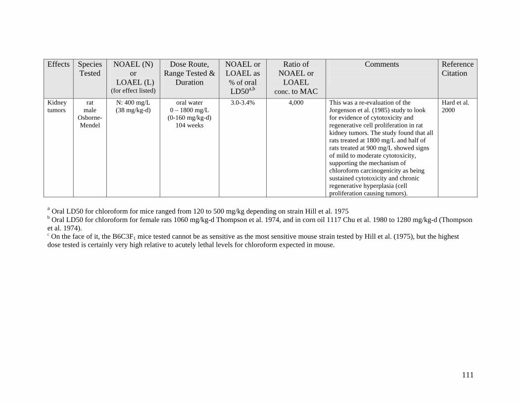
111

Effects Species Tested

NOAEL (N) or

LOAEL (L) (for effect listed)

Dose Route, Range Tested &

Duration

NOAEL or LOAEL as % of oral LD50a,b

Ratio of NOAEL or

LOAEL conc. to MAC

Comments

Reference Citation

Kidney tumors

rat male

Osborne-Mendel

N: 400 mg/L (38 mg/kg-d)

oral water 0 – 1800 mg/L

(0-160 mg/kg-d) 104 weeks

3.0-3.4% 4,000 This was a re-evaluation of the Jorgenson et al. (1985) study to look for evidence of cytotoxicity and regenerative cell proliferation in rat kidney tumors. The study found that all rats treated at 1800 mg/L and half of rats treated at 900 mg/L showed signs of mild to moderate cytotoxicity, supporting the mechanism of chloroform carcinogenicity as being sustained cytotoxicity and chronic regenerative hyperplasia (cell proliferation causing tumors).

Hard et al. 2000

a Oral LD50 for chloroform for mice ranged from 120 to 500 mg/kg depending on strain Hill et al. 1975 b Oral LD50 for chloroform for female rats 1060 mg/kg-d Thompson et al. 1974, and in corn oil 1117 Chu et al. 1980 to 1280 mg/kg-d (Thompson et al. 1974). c On the face of it, the B6C3F1 mice tested cannot be as sensitive as the most sensitive mouse strain tested by Hill et al. (1975), but the highest dose tested is certainly very high relative to acutely lethal levels for chloroform expected in mouse.

112

Table A1-2 Long Term Cancer Studies on Bromodichloromethane (BDCM) Effects Species

Tested NOAEL (N)

or LOAEL (L) (for effect listed)

Dose Route, Range Tested &

Duration

NOAEL or LOAEL as % of oral LD50a,b

Ratio of NOAEL or

LOAEL conc. to MAC

Comments

Reference Citation

Liver tumors

mouse both sexes

B6C3F1

L: 75 mg/kg-d corn oil gavage dosing 5 d/week female (mg/kg-d)

0, 75 “low dose”,

150 “high dose” male (mg/kg-d)

0, 50 “low dose”,

100 “high dose” 102 weeks

7.7% not applicable gavage

In female mice, the incidences of adenomas and adenomas and carcinomas combined were significantly higher in the low dose group than the control.

NTP 1987

Liver tumors

rat both sexes

Osborne-Mendel

N: 100 mg/kg-d corn oil gavage dosing 5 d/week female (mg/kg-d)

0, 50 “low dose”,

100 “high dose” male (mg/kg-d)

0, 50 “low dose”,

100 “high dose” 102 weeks

10-11% not applicable gavage

One high dosed male showed a liver tumor, but this was not statistically significant relative to the control. Necrosis was observed at slightly increased incidence in dosed male rats. Cellular changes were observed in high dose female rats. Fatty metamorphosis was observed at increased incidences in dosed male and female rats.

NTP (1987)

Liver tumors

rat male

F344/N rats

L: 3.9 mg/kg-d

oral water dosing continuous

0 – 620 mg/L (0 – 36.3 mg/kg-d)

78 weeks

4% 39,000 Excess liver tumors occurred at doses of 3.9 and 20.6 mg/kg-d but tumor prevalence and multiplicity declined at the highest dose level (36.3 mg/kg-d)

George et al. 2002

113

Effects Species Tested

NOAEL (N) or

LOAEL (L) (for effect listed)

Dose Route, Range Tested &

Duration

NOAEL or LOAEL as % of oral LD50a,b

Ratio of NOAEL or

LOAEL conc. to MAC

Comments

Reference Citation

Liver tumors

mouse male

B6C3F1

N: 43.4 mg/kg-d

oral water dosing continuous

0 – 490 mg/L (0 – 43.4 mg/kg-d)

78 weeks

4.6% 31,000 No increase in liver tumors at any dose George et al. (2002)

Liver tumors

mouse female

B6C3F1

N: 700 mg/L (36 mg/kg-d)

oral water 0 – 700 mg/L

(0-36 mg/kg-d) 104 weeks

3.8% 44,000 Incidence of hepatocellular adenoma or carcinoma combined decreased relative to the control and the highest dose group was significantly reduced relative to the control

NTP 2006

Liver tumors

rat male

F344/N

N: 700 mg/L (25 mg/kg-d)

oral water 0 – 700 mg/L

(0-25 mg/kg-d) 104 weeks

2.7% 44,000 Chronic inflammation of the liver in the 350 and 700 mg/L dose groups was significantly greater than controls, but no increased incidence of liver tumors could be attributed to BDCM dosing

NTP (2006)

Kidney tumors

mouse both sexes

B6C3F1

N: 25 mg/kg-d corn oil gavage dosing 5 d/week female (mg/kg-d)

0, 75 “low dose”,

150 “high dose” male (mg/kg-d)

0, 25 “low dose”, 50 “high dose”

102 weeks

2.7% not applicable gavage

No renal cell tumors were diagnosed in females. Renal tubular cell adenomas or adenocarcinomas combined increased with dose and were significantly greater than controls in the high dose.

NTP (1987)

114

Effects Species Tested

NOAEL (N) or

LOAEL (L) (for effect listed)

Dose Route, Range Tested &

Duration

NOAEL or LOAEL as % of oral LD50a,b

Ratio of NOAEL or

LOAEL conc. to MAC

Comments

Reference Citation

Kidney tumors

rat both sexes

Osborne-Mendel

N: 50 mg/kg-d corn oil gavage dosing 5 d/week female (mg/kg-d)

0, 50 “low dose”,

100 “high dose” male (mg/kg/d)

0, 50 “low dose”,

100 “high dose” 102 weeks

5.5% not applicable gavage

For both males and females, renal tubular cell adenomas or adenocarcinomas combined increased with dose and were significantly greater than controls in the high dose.

NTP (1987)

Kidney tumors

rat male

F344/N rats

N: 620 mg/L (36.3 mg/kg-d)

oral water dosing continuous

0 – 620 mg/L (0 – 36.3 mg/kg-d)

78 weeks

4% 39,000 No increase in kidney tumors was observed in this study.

George et al. (2002)

Kidney tumors

mouse male

B6C3F1

N: 490 mg/L (43.4 mg/kg-d)

oral water dosing continuous

0 – 490 mg/L (0 – 43.4 mg/kg-d)

78 weeks

4.6% 31,000 No increase in kidney tumors at any dose

George et al. (2002)

Kidney tumors

mouse female

B6C3F1

N: 700 mg/L (36 mg/kg-d)

oral water 0 – 700 mg/L

(0-36 mg/kg-d) 104 weeks

3.8% 44,000 No increase in kidney tumors at any dose

NTP (2006)

Kidney tumors

rat male

F344/N

N: 700 mg/L (25 mg/kg-d)

oral water 0 – 700 mg/L

(0-25 mg/kg-d) 104 weeks

2.7% 44,000 There were no tumors attributed to BDCM exposure.

NTP (2006)

115

Effects Species Tested

NOAEL (N) or

LOAEL (L) (for effect listed)

Dose Route, Range Tested &

Duration

NOAEL or LOAEL as % of oral LD50a,b

Ratio of NOAEL or

LOAEL conc. to MAC

Comments

Reference Citation

Large intestine tumors

rat both sexes

Osborne-Mendel

L: 50 mg/kg-d corn oil gavage dosing 5 d/week female (mg/kg-d)

0, 50 “low dose”,

100 “high dose” male (mg/kg-d)

0, 50 “low dose”,

100 “high dose” 102 weeks

5.5% not applicable gavage

Adenosarcomas were significantly greater at low and high dose compared with controls for males

NTP (1987)

Large intestine tumors

rat male

F344/N rats

N: 620 mg/L (36.3 mg/kg-d)

oral water dosing continuous

0 – 620 mg/L (0 – 36.3 mg/kg-d)

78 weeks

4% 39,000 No increase in tumors of the large bowel was observed in this study. Only one such tumor was observed in a control animal

George et al. (2002)

Large intestine tumors

rat male

Osborne-Mendel

N: 700 mg/L (25 mg/kg-d)

oral water 0 – 700 mg/L

(0-25 mg/kg-d) 104 weeks

2.7% 44,000 There were no tumors attributed to BDCM exposure.

NTP (2006)

a Oral LD50 for BDCM in Sprague Dawley rats: female 969 mg/kg-d and male 916 mg/kg-d (Chu et al. 1980) b Oral LD50 for BDCM for mice not found, mean value (943 mg/kg-d) for rat from Chue et al. (1980) used

116

Table A1-3 Long Term Cancer Studies on Haloacetic Acids Effects Species

Tested NOAEL (N)

or LOAEL (L) (for effect listed)

Dose Route, Range Tested &

Duration

NOAEL or LOAEL as % of oral

LD50

Ratio of NOAEL or

LOAEL conc. to MAC

Comments

Reference Citation

Dichloroacetic acid oral LD50 = 5000 mg/kg in rodents (Stacpoole et al. 1998) Liver tumors

mouse both sexes

B6C3F1

L: 1000 mg/L (170 mg/kg-d)

oral drinking water

0, 1000, 2000 mg/L (170 mg/kg-d, 340 mg/kg-d)

up to 52 weeks

3.4 % 12,500 Hepatocelluar tumors were induced at 2000 mg/L in male, but not in female mice. The tumorigenic response was attributed to hepatomegaly and associated focal necrotic lesions

Bull et al. 1990

Liver tumors

mouse male

B6C3F1

L: 50 mg/L (8 mg/kg-d)

oral drinking water

0, 50, 500, 1000, 2000 or 3500 mg/L (8, 84, 168, 315, or

429 mg/kg-d) 90 -100 weeks

0.16% 625 Hepatocelluar tumor multiplicity (tumors per animal) was increased at all dose levels compared with the control. Cumulative incidence of hepatocellular tumors was significantly increased in mice exposed to doses of 1000 mg/L and above

DeAngelo et al. 1999

Liver tumors

rat male

F344/N

N: 50 mg/L 3.6 mg/kg-d

oral drinking water

50, 500, 1600 mg/L (3.6, 40, 139

mg/kg-d) 100 weeks

0.07% 625 DeAngelo et al. 1996

117

Effects Species Tested

NOAEL (N) or

LOAEL (L) (for effect listed)

Dose Route, Range Tested &

Duration

NOAEL or LOAEL as % of oral

LD50

Ratio of NOAEL or

LOAEL conc. to MAC

Comments

Reference Citation

Trichloroacetic acid oral LD50 = 5000 mg/kg in rats (Bailey and White 1965) Residue Review 10: 97. Liver tumors

mouse both sexes

B6C3F1

L: 1000 mg/L (164 mg/kg-d)

drinking water 0, 1000, 2000 mg/L

(164 mg/kg-d, 329 mg/kg-d)

up to 52 weeks

3.3 % 12,500 Hepatocelluar tumors were induced at both trichloracetic acid doses in male, but not in female mice but the findings were not statistically significant relative to the controls.

Bull et al. (1990)

Liver tumors

rat male

F344/N

N: 5000 mg/L (364 mg/kg-d)

oral water dosing continuous

50, 500, 5000 mg/L (3.6, 32.5, 364

mg/kg-d) 100 weeks

7.3% 62,500 No evidence of tumors relative to controls at any site for any dose level

DeAngelo et al. 1997

118

Appendix A2 Epidemiology Studies of Cancer and Chlorination DBPs

119

Table A2-1 Epidemiology Studies of Cancer Sites Other Than Bladder, Colon or Rectum Study Citation

Dates Study Design

Location Sample size & type

OR (CI) & Association

Dose- response

Duration response

Exposure Assessment

Do et al. 2005

1994-1997

Case-control; population- based

Alberta, British Columbia, Manitoba, Nova Scotia, Ontario and Saskatchewan, Canada

486 incident cases of pancreatic cancer with 3,596 matched population-based contols

0.86 (0.58 – 1.28)

Negative (NS)

No No THM data from 4 surveys conducted in 1975, 1988 and 1995 were used to estimate THM levels by municipal water supply which was assumed to apply to all residents equally and these estimates were linked to case residence based on an individual questionnaire.

Kasim et al. 2006

1994-1997

Case-control; population- based

Canada, all provinces except Quebec and New Brunswick

686 incident leukemia cases and 3420 controls for whom water quality information was available for at least 30 years

All adult leukemia

0.77 (0.59 – 1.02) negative (NS)

chronic

myelocytic L 1.72

(1.01 – 3.08) positive*

No

No

No

Yes

Multiple information sources on THM levels for community water supplies, varying from one province to another were integrated with municipal water inventories that described changes in water treatment practice to create a linear regression model to estimate THM exposure levels by treatment plant. Each individual exposure was assigned according to subject’s residence and water source history linked to the THM data model by geographic area and time.

120

Study Citation

Dates Study Design

Location Sample size & type

OR (CI) & Association

Dose- response

Duration response

Exposure Assessment

Infante-Rivard et al. 2002

1980-1993

Case-only within previous Case-control

Québec, Canada

170 incident cases of childhood acute lymphoblastic leukemia were evaluated for genetic markers of relevant metabolic enzyme systems, GSTT1 and CYP2E1*5

Interaction Odds Ratio

IOR 9.1

(1.4 – 57.8) GSTT1 null

IOR 9.7

(1.1 – 86) CYP2E1*5

N/A N/A The exposure assessment was drawn from Infante-Rivard et al. (2001) and was combined with the assessment of genetic markers to determine if these markers affected the interaction odds ratio (IOR)

Infante-Rivard et al. 2001

1980-1993

Case-control; population-based

Québec, Canada

491 incident cases of childhood acute lymphoblastic leukemia with 491 controls

1.54 (0.78 – 3.03) positive (NS)

No N/A A questionnaire to 305 municipalities where either cases or controls had resided to obtain monitoring data on THMs, metals and nitrates. Ministry of Environment monitoring data was obtained for these parameters for distribution system samples and samples were collected in 227 homes of cases and controls. Residential histories were collected on cases and controls and used with an exposure matrix to develop exposure indices

121

Study Citation

Dates Study Design

Location Sample size & type

OR (CI) & Association

Dose- response

Duration response

Exposure Assessment

Tao et al. 1999

1984 - 1988

Case – control; population- based; death certificate

Shanghai region, China

71 esophageal cancer deaths matched with 1122 controls (1% random sample of defined cohort living at the end of the 5 year follow-up)

2.77 (1.52 – 5.03)

Positive*

No N/A Mutagenicity of drinking water was determined based on Ames tests on water samples collected between 1983 and 1985. Both raw and chlorinated tap water from Shanghai were uniformly positive for mutagenicity with average chloroform of 45.6 µg/L, while both raw and chlorinated water from an upstream plant were negative with an average chloroform of 1.1 µg/L. Drinking water source for cases and controls was assigned by residential address served by the mutagenic downstream water vs. non-mutagenic upstream water

Cantor et al. 1999

1984- 1987

Case – control; population- based

Iowa, U.S.A.

375 incident brain cancer cases with 2,434 controls of whom 291 cases and 1983 controls had water quality information for at least 70% of individual lifetime.

Male 2.5

(1.2 – 5.0) positive*

Female

0.7 (0.3 – 1.6) Negative

Male Yes

Female No

Male Yes

Female No

A survey of all water utilities serving at least 1000 population engaged 280 utilities serving 280 communities with a combined population of 1.94 million. In addition to interviews and questionnaire completion 1 or 2 water samples were collected for THM analysis. The water utility characteristics and THM monitoring data were combined with personal questionnaire data on residential location and water consumption to develop THM exposure indices for each participant.

122

Study Citation

Dates Study Design

Location Sample size & type

OR (CI) & Association

Dose- response

Duration response

Exposure Assessment

Koivusalo et al. 1998a

1991-1992

Case – control, population-based

Finland 703 incident cases of kidney cancer with 914 population controls

Men 1.47

(1.04 – 2.06) Positive*

Women

1.03 (0.68 – 1.55)

(NS)

Men Yes

Women No

Men No

Women No

Exposure to an estimate of mutagenicity of municipal drinking water based on a model that predicts a mutagenicity level (Ames Salmonella assay) based on a combination of water quality parameters. Effects of age, gender, exclusion of cities with substantial proportions of chemical, pulp & paper or agricultural workers and social structure were made.

Marcus et al. 1998

1990-1992

Aggregate Ecologic

North Carolina

6,462 cases of breast cancer were used to estimate incidence rates

Not associated N/A N/A 71 water suppliers serving at least 10,000 customers provided quarterly THM data for April 1993 to March 1994 to allow estimation of THM exposure for each supplier. Zipcodes were assigned to each supplier and used as the basis for calculating breast cancer incidence rates.

Kukkula and Lofroth 1997

1989-1991

Case-control; population-based

Finland, Turku region

For a population study base of 220,000, 183 incident cases of pancreatic cancer were each had 2 randomly selected matched controls

0.20 (0.04 – 0.94)

negative*

N/A Yes negative

Exposure was estimated on whether the subject was served by a chlorinated water supply for residential address (1 year minimum) up to 20 years prior to diagnosis

123

Study Citation

Dates Study Design

Location Sample size & type

OR (CI) & Association

Dose- response

Duration response

Exposure Assessment

Koivusalo et al. 1997

1971-1993

Cross-sectional*

Finland, 56 urban municipalities

Total population of 621,431 persons. Evaluated for 23 cancer sites

multiple N/A N/A Exposure to an estimate of mutagenicity of municipal drinking water based on a model that predicts a mutagenicity level (Ames Salmonella assay) based on a combination of water quality parameters. Effects of age, gender, exclusion of cities with substantial proportions of chemical, pulp & paper or agricultural workers and social structure were made.

Koivusalo et al. 1995

1966 - 1976; 1977 - 1989

Cross-sectional*

Finland, 56 urban municipalities

Total population not provided. Evaluated for incident cases at cancer sites of: liver pancreatic and soft-tissue cancers Hodgkin’s disease Hon-Hodgkin’s lymphoma and leukemia

multiple N/A N/A Exposure to an estimate of mutagenicity of municipal drinking water based on a model that predicts a mutagenicity level (Ames Salmonella assay) based on a combination of water quality parameters. Effects of age, gender, exclusion of cities with substantial proportions of chemical, pulp & paper or agricultural workers and social structure were made.

124

Study Citation

Dates Study Design

Location Sample size & type

OR (CI) & Association

Dose- response

Duration response

Exposure Assessment

Ijsselmuiden et al. 1992

1975-1989

Case – control; population-based

Washington County, Maryland, U.S.A.

101 incident cases of pancreatic cancer with 206 population controls

2.18 (1.2 – 3.95)

positive*

N/A N/A Municipal sources were predominantly chlorinated while only 6% of non-municipal sources were chlorinated. Limited THM monitoring on the largest municipal source showed THM levels often exceeded 100 g/l prior to the introduction of filtration in 1979. Exposure was compared between municipal and non-municipal sources.

Fagliano et al. 1990

1979-1984

Aggregate Ecologic

New Jersey, U.S.A.

Standardized incident ratios (SIR) were calculated for 372 incident cases (208 male, 164 female) of leukemia

N/A N/A N/A Data for 14 volatile organic compounds (VOC) and THM were collected in the water systems serving the study area in 1984 and 1985. The water systems were stratified according to high, medium and low for the non-THM VOC and into high and low for THM. The calculated SIR were compared for the different exposure categories

125

Table A2-2 Epidemiology Studies Including Colon and/or Rectal Cancer Study Citation

Dates Study Design

Location Sample size & type

OR (CI) & Association

Dose- response

Duration response

Exposure Assessment

Bove et al. 2007a

1979-1985

Case-control; population- based

Monroe County, New York, U.S.A.

128 cases of rectal cancer and 253 matched controls.

Rectal 2.32

(1.22 – 4.39) positive*

for bromoform which is

typically very low

No

N/A Data provided by the Monroe County Water Authority and the Monroe County Health Department were used to determine THM exposure using two different exposure models, with one considering travel time in the water distribution system. These models predicted THM exposure by geographic location that was combined with residential histories obtained by interview of study subjects.

King et al. 2000b

1992- 1994

Case-control: population-based

Ontario, Canada

767 incident colon cancer cases and 661 incident rectal cancer cases were matched with 1545 controls.

Colon Male 1.87

(1.15 – 3.05) positive (NS)

Female 0.92

(0.49 – 1.71) Negative (NS)

Rectal Male 0.98

(0.56 – 1.72) negative (NS)

Female

1.09 (0.75 – 1.57) positive (NS)

Colon Male Yes

Female Yes

Rectal Male No

Female No

Colon Male Yes

Female Yes

Rectal Male No

Female No

A database was created for each drinking water supply including source (surface or groundwater) and chlorination status. A model was constructed to estimate THM level based on data from the Ontario Drinking Water Surveillance program (1986 – 1992) which was used to estimate THM levels from 1950 to 1990. Subjects were interviewed about water consumption 2 years prior and to provide water exposure history for at least 30 years. Exposure levels were assigned according to water source and modeled THM estimates for identified water sources.

126

Study Citation

Dates Study Design

Location Sample size & type

OR (CI) & Association

Dose- response

Duration response

Exposure Assessment

Hildesheim et al. 1998

1986- 1989

Case-control; population-based

Iowa, U.S.A.

Odds ratios were calculated for 560 colon and 537 rectal cancer cases with 1983 controls for whom water exposure information was available for at least 70% of subject lifetime.

Colon 1.13

(0.7 – 1.8) positive (NS)

Rectal

1.7 (1.1 – 2.6) positive*

Colon No

Rectal Yes

Colon No

Rectal Yes

Water from private wells was assumed to be non-chlorinated, Iowa water utilities serving at least 1000 residents (approximately 2/3 of state population) were surveyed for historical information and were sampled for THMs. These data were combined with individual questionnaire data (including 210 proxy interviews) to derive several THM exposure indices.

Doyle et al. 1997

1986-1993

Cohort prospective

Iowa, U.S.A.

Women aged 55 to 69 on 1985 drivers’ license list. 36,127 answered a questionnaire regarding water use. The cohort was followed up for 12 cancer sites with: colon (178), rectum & anus (78) and bladder (42)

Female Colon 1.68

(1.11 – 2.53) positive*

Rectal 1.07

(0.60 – 1.93) positive (NS)

Female Colon Yes

Rectal Yes

Female Colon N/A

Rectal Yes

Qualitative water source assignments of participants were made to 4 groups: municipalities on 100% groundwater, municipalities on mixed ground and surface water, municipalities on 100% surface water and private well water. Exposure levels assigned to these categories were estimated based on two state-wide surveys done in 1979 and 1986 on 252 municipal water supplies in Iowa.

127

Study Citation

Dates Study Design

Location Sample size & type

OR (CI) & Association

Dose- response

Duration response

Exposure Assessment

Koivusalo et al. 1994

1967-1986

Aggregate Ecologic

56 Counties in Finland

32,551 incident cancer cases including: bladder (4144), colon (7233) and rectum (5253) used to calculate age-adjusted incident rates

N/A N/A N/A Exposure to an estimate of mutagenicity of municipal drinking water based on a model that predicts a mutagenicity level (Ames salmonella assay) based on a combination of water quality parameters. Assessments were made against water exposures classified as no mutagenicity, mutagenicity at less than 3000 revertants per L and for mutagenicity greater than 3000 revertants per L.

Hoff et al. 1992

>1984 Screening study

Telemark, Norway

324 volunteers to undergo fibre-optic screening for polyps in the rectum and sigmoid colon

colorectal polyps are not

associated with drinking

water chloroform

N/A N/A 310 volunteers received drinking water from 1 of 4 major water supplies, all of which used chlorine for disinfection. Various water quality parameters, including chloroform were analyzed for correlation with the occurrence of polyps, but chloroform levels were virtually identical in all 4 water supplies.

Flaten 1992 1975-1984

Aggregate Ecologic

Norway Age adjusted cancer incidence rates were calculated for 15 cancer sites including bladder, colon and rectal cancer

N/A N/A N/A 96 municipalities (excluding Oslo) were categorized as chlorinated municipalities, non-chlorinating municipalities (no chlorinated water ever delivered) and partly chlorinating municipalities. Cancer incidence rates by municipality were compared with water supply category.

128

Study Citation

Dates Study Design

Location Sample size & type

OR (CI) & Association

Dose- response

Duration response

Exposure Assessment

Young et al. 1987

1982-1983

Case-control; population & hospital-based

Wisconsin, U.S.A.

347 incident colon cancer cases with 639 cancer controls and 611 population controls

Colon 0.73

(0.44 – 1.21) negative (NS)

Colon No

Colon No

THM4 monitoring data was collected seasonally for 1 year at 81 waterworks comprising sources as: 14 Great Lakes, 5 other surface and 63 groundwater. The combination of monitoring and survey data from each plant were used to construct a model to estimate THM exposure levels back over time. A dichotomous variable of surface vs. groundwater and chlorine disinfection (yes or no) were used in the analysis.

Richmond et al. 1987

1976-1980

Aggregate Ecologic

Campbell County, Kentucky, U.S.A.

254 incident cases of colorectal cancer were used to calculate standardized incidence ratios.

N/A N/A N/A THM4 concentrations in drinking water sourced from the Ohio River averaged 170 µg/L (range 160 to 220 µg/L) compared with individual cisterns (rainwater) and private well supplies, which averaged 7 µg/L (range 0 to 12 µg/L)

Zierler et al. 1986

1969-1983

Aggregate Ecologic

Massachusetts, U.S.A.

51,645 cancer deaths including: colon (10,517), and rectum (2700) and 214,988 controls deaths from non-cancer or lymphatic cancers.

Colon 0.89

(0.86 – 0.93) negative*

Rectal 0.96

(0.89 – 1.04)

Colon N/A

Rectal N/A

Colon N/A

Rectal N/A

Community water treatment systems were categorized as using chlorination or chloramination and subjects were classified according to last residence before death as being either a chlorinated or a chloraminated water supply. Standardized incidence ratios for colon and rectum were compared by water source.

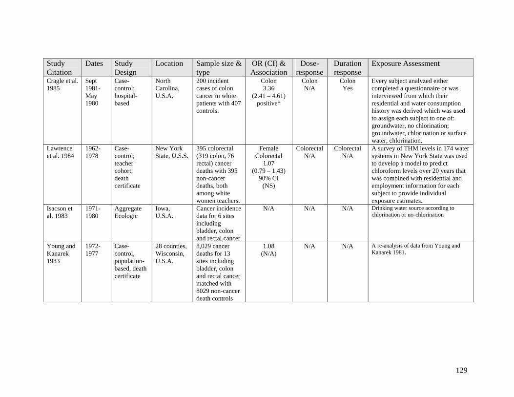
129

Study Citation

Dates Study Design

Location Sample size & type

OR (CI) & Association

Dose- response

Duration response

Exposure Assessment

Cragle et al. 1985

Sept 1981-May 1980

Case-control; hospital-based

North Carolina, U.S.A.

200 incident cases of colon cancer in white patients with 407 controls.

Colon 3.36

(2.41 – 4.61) positive*

Colon N/A

Colon Yes

Every subject analyzed either completed a questionnaire or was interviewed from which their residential and water consumption history was derived which was used to assign each subject to one of: groundwater, no chlorination; groundwater, chlorination or surface water, chlorination.

Lawrence et al. 1984

1962-1978

Case-control; teacher cohort; death certificate

New York State, U.S.S.

395 colorectal (319 colon, 76 rectal) cancer deaths with 395 non-cancer deaths, both among white women teachers.

Female Colorectal

1.07 (0.79 – 1.43)

90% CI (NS)

Colorectal N/A

Colorectal N/A

A survey of THM levels in 174 water systems in New York State was used to develop a model to predict chloroform levels over 20 years that was combined with residential and employment information for each subject to provide individual exposure estimates.

Isacson et al. 1983

1971-1980

Aggregate Ecologic

Iowa, U.S.A.

Cancer incidence data for 6 sites including bladder, colon and rectal cancer

N/A N/A N/A Drinking water source according to chlorination or no-chlorination

Young and Kanarek 1983

1972-1977

Case-control, population-based, death certificate

28 counties, Wisconsin, U.S.A.

8,029 cancer deaths for 13 sites including bladder, colon and rectal cancer matched with 8029 non-cancer death controls

1.08 (N/A)

N/A N/A A re-analysis of data from Young and Kanarek 1981.

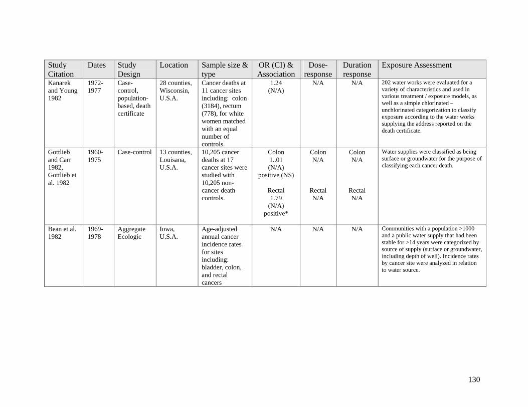
130

Study Citation

Dates Study Design

Location Sample size & type

OR (CI) & Association

Dose- response

Duration response

Exposure Assessment

Kanarek and Young 1982

1972-1977

Case-control, population-based, death certificate

28 counties, Wisconsin, U.S.A.

Cancer deaths at 11 cancer sites including: colon (3184), rectum (778), for white women matched with an equal number of controls.

1.24 (N/A)

N/A N/A 202 water works were evaluated for a variety of characteristics and used in various treatment / exposure models, as well as a simple chlorinated – unchlorinated categorization to classify exposure according to the water works supplying the address reported on the death certificate.

Gottlieb and Carr 1982, Gottlieb et al. 1982

1960-1975

Case-control 13 counties, Louisana, U.S.A.

10,205 cancer deaths at 17 cancer sites were studied with 10,205 non-cancer death controls.

Colon 1..01 (N/A)

positive (NS)

Rectal 1.79

(N/A) positive*

Colon N/A

Rectal N/A

Colon N/A

Rectal N/A

Water supplies were classified as being surface or groundwater for the purpose of classifying each cancer death.

Bean et al. 1982

1969-1978

Aggregate Ecologic

Iowa, U.S.A.

Age-adjusted annual cancer incidence rates for sites including: bladder, colon, and rectal cancers

N/A N/A N/A Communities with a population >1000 and a public water supply that had been stable for >14 years were categorized by source of supply (surface or groundwater, including depth of well). Incidence rates by cancer site were analyzed in relation to water source.

131

Study Citation

Dates Study Design

Location Sample size & type

OR (CI) & Association

Dose- response

Duration response

Exposure Assessment

Wilkins and Comstock 1981

1963- 1975

Cross-sectional mortality survey, death certificate

Washington County Maryland, U.S.A.

122 colon cancer deaths and 63 rectal cancer deaths analyzed by residence

Colon 0.89

(0.57 – 1.43) Negative (NS)

Rectal 1.42

(0.70 – 3.16) positive (NS)

Colon N/A

Rectal N/A

Colon N/A

Rectal N/A

Drinking water exposure that were analyzed for association with causes of death were classified into 2 groups: Hagerstown residents (chlorinated surface water) and deep well users (non-chlorinated. A census had determined drinking water source by address for 98% of households, thereby allowing assignment of water exposure according to residential address.

Young et al. 1981

1972-1977

Case-control, population-based, death certificate

28 counties, Wisconsin, U.S.A.

8,029 cancer deaths for 13 sites including bladder and rectal cancer matched with 8029 non-cancer death controls

Female Colon 1.51

(1.06 – 2.14) Positive*

Rectal 1.39

(0.67 – 2.86) Positive (NS)

Colon

No

Rectal yes

Colon N/A

Rectal N/A

Waterworks survey data in 1970 (based on data for 1960-1965) were used along with results from a questionnaire sent to waterworks superintendents to allow categorization of waterworks into high, medium and low chorine dosage. The residence listed on the death certificate for each case and control was used to assign a waterworks chlorine dose exposure.

Gottlieb et al. 1981

1960-1975

Case-control, population-based, death certificate

20 counties, Louisana, U.S.A.

1167 colon and 692 rectal cancer deaths were studied with an equal number of matched controls.

Male Colon 2.07

(1.49 – 2.88) Positive*

Rectal 0.96

(0.75 – 1.24) negative (NS)

Colon Yes

Rectal No

Colon N/A

Rectal N/A

Water supplies were classified as being: mostly surface, some surface, possible surface and least surface for the purpose of categorizing the cancer cases according to residence listed on the death certificate.

132

Study Citation

Dates Study Design

Location Sample size & type

OR (CI) & Association

Dose- response

Duration response

Exposure Assessment

Brenniman et al. 1980

1973-1976

Case-control, population-based, death certificates

Illinois, U.S.A.

3208 white cancer deaths for sites including: large intestine 1237, rectum 295 and bladder 284, with 43,666 control deaths.

Colon 1.11

(N/A) Positive (NS)

Rectal 1.22

(N/A) Positive (NS)

Colon N/A

Rectal N/A

Colon N/A

Rectal N/A

For a total of 542 communities using groundwater, 272 were chlorinated and 270 were non-chlorinated. Comparsions were made between these exposure categoriess.

Carlo and Mettlin 1980

1973-1976

Aggregate Ecologic

Erie County, New York, U.S.A.

4255 cases for sites including: colon, rectal, and bladder cancers were analyzed for incidence rates.

N/A N/A N/A THM4 was measured at water treatment plants in July 1978 (range 0 – 71 µg/L, mean 46 µg/L ). Correlation of the specified cancer incidence rates was determined with various demographic factors, water source type (surface – lake, river or reservoir or ground – well or spring).

Cantor et al. 1978

1968-1971

Aggregate Ecologic

923 Counties (>50% urban) U.S.A.

Average annual age-adjusted mortality rates were calculated for 22 cancer sites including bladder, colon and rectal cancer.

N/A N/A N/A Chloroform and THM4 levels for major municipal water supplies were derived by a nation-wide survey conducted by the U.S. EPA in 1975 and a survey done in U.S. EPA Region V. Correlations were calculated between cancer mortality rates and THM4, chloroform or brominated THMs (by difference) for geographic regions where the majority of the water was provided by a sampled water supply.

Alavanja et al. 1978

1968-1970

Case-control, population-based, death certificates

7 Counties, New York State, U.S.A.

3446 gastrointestinal and urinary tract cancer deaths with 3444 matched controls

Colon 1.61 (NA)

positive*

Rectal 1.93 (NA)

positive*

Colon N/A

Rectal N/A

Colon N/A

Rectal N/A

Exposures were categorized as urban or rural, as well as for chlorinated vs. non-chlorinated and surface vs. groundwater sources using detailed water distribution maps to assign these exposures to geographic location for cases and controls.

133

Study Citation

Dates Study Design

Location Sample size & type

OR (CI) & Association

Dose- response

Duration response

Exposure Assessment

Kuzma et al. 1977

1950-1969

Aggregate Ecologic

88 Counties, Ohio, U.S.A.

Age-adjusted cancer rates for 8 cancer sites including: large intestine, rectum, and bladder

N/A N/A N/A A U.S. Public Health Service inventory of water supplies in Ohio counties was used to assign exposure as being surface water or groundwater.

134

Table A2-3 Epidemiology Studies Including Bladder Cancer Study Citation

Dates Study Design

Location Sample size & type

OR (CI) & Association

Dose- response

Duration response

Exposure Assessment

Villanueva et al. 2007

1998 - 2001

Case-control: hospital-based

Spain, 18 hospitals in 5 geographic regions

1219 incident bladder cancer cases and 1271 matched controls.

2.10 (1.09 – 4.02)

positive

yes no Based on 113 tap water samples in the study area in 1999 and a questionnaire submitted to approx. 200 water companies, data on THM levels, water source history (proportion of ground / surface water over time) and the year chlorination was implemented was initiated to estimate THM levels. Interview questionnaires covered residential history from birth, water source at each residence, average daily water consumption, frequency, duration and water temperature of bathing / showering and frequency, duration and location of swimming pool attendance.

Michaud et al. 2007

1998- 2001

Case- control: hospital-based

Spain, 18 hospitals in 5 geographic regions

397 bladder cancer cases and 664 matched controls.

2.06 (0.83 – 5.08) Positive (NS)

no N/A See Villaneuva et al. (2007)

Bove et al. 2007b

1979-1985

Case-control; population- based

3 counties in western New York state, U.S.A.

182 bladder cancer cases and 385 matched controls

2.34 (1.01 – 3.66)

Positive

Stronger response found for bromoform

and for exposure to longer water

travel time

yes N/A Data provided by County Health Department involving 7 to 10 samples per year at approximately 65 sites were used to estimate average THM levels spatially. These data showed a strong impact of distribution system travel time. These THM estimates by geographic location were combined with residential histories obtained by interview of study subjects.

135

Study Citation

Dates Study Design

Location Sample size & type

OR (CI) & Association

Dose- response

Duration response

Exposure Assessment

Chang et al. 2007

1996-2005

Case-control; population- based; death certificate

Taiwan, 65 municipalities

403 bladder cancer deaths and 403 population matched controls

2.11 (1.43 – 3.11)

positive

yes N/A Quarterly THM4 samples were collected over 2 years for each of 65 municipalities and the average THM4 level over this period was assigned to each subject according to the residence listed on the death certificate for each case or control

Chevrier et al. 2004

1985-87 Case-control; hospital-based

7 French hospitals

281 cases and 272 controls

2.99 (1.1-8.5)

Yes Yes This study took advantage of the common use of ozonation in France to obtain a range of exposures to chlorination DBPs, but THM levels used were estimated by an elaborate expert Delphi procedure for construction of THM exposure histories rather than any THM monitoring data

Vinceti et al. 2004

1987- 1999

Aggregate Ecological

Guastalla, Italy

Mortality was assessed among a cohort of 5144 residents to estimate standardized motrality ratios for 15 cancer sites including bladder, colon and rectum

N/A N/A N/A The cohort were defined as residing in the Guastalia region where they were exposed to chlorinated well water from 1965 to 1987 with THM4 measured as high as 71 µg/L in 1984. The standardized mortality ratios were compared with a referent population in Reggio Emilia (approx 140,000) where THM levels in drinking water were generally at or below the detection limit.

Ranmuthugala et al. 2003

1997 Prospective cohort

3 sites, Australia

348 completed the study and 228 had slides suitable

N/A N/A N/A Three communities provided water supplies with zero exposure to THMs, medium exposure (median THM at 64 µg/L) and high exposure (median THM at 138 µg/L). Mean number of micronuclei (per 1000 normal cells) were evaluated against concentration and mass ingestion of individual THM and THM4.

136

Study Citation

Dates Study Design

Location Sample size & type

OR (CI) & Association

Dose- response

Duration response

Exposure Assessment

Cantor et al. 1998

1986-1989

Case – control, population-based

Iowa, U.S.A.

1123 incident bladder cancer cases with 1983 controls

1.5 (0.9 – 2.6)

Positive (NS)

yes yes A survey of all water utilities serving at least 1000 population engaged 280 utilities serving 280 communities with a combined population of 1.94 million. In addition to interviews and questionnaire completion 1 or 2 water samples were collected for THM analysis. The water utility characteristics and THM monitoring data were combined with personal questionnaire data on residential location and water consumption to develop THM exposure indices for each participant.

Koivusalo et al. 1998b

1991-1992

Case – control, population-based

Finland 732 incident cases of bladder cancer, 703 incident cases of kidney cancer with 914 population controls

1.22 (0.92 – 1.62) Positive (NS)

no yes Exposure to an estimate of mutagenicity of municipal drinking water based on a model that predicts a mutagenicity level (Ames salmonella assay) based on a combination of water quality parameters. Effects of age, gender, exclusion of cities with substantial proportions of chemical, pulp & paper or agricultural workers and social structure were made.

Yang et al. 1998

1982-1991

Aggregate Ecologic

Taiwan Age adjusted mortality rates for various cancers including bladder, colon and rectal cancer

N/A N/A N/A Of Taiwan’s 361 administrative units, 310 were considered for this study to determine chlorination status. 156 of these municipalities were regarded as having more than 90% of the municipality served by chlorinated water. Non-chlorinating municipalities were those with less than 5% of the population served chlorinated water and 15 qualified. From these, 14 non-chlorinating municipalities were matched, on the basis of urbanization, with 14 chlorinating municipalities to perform the ecological assessment of cancer mortality rates.

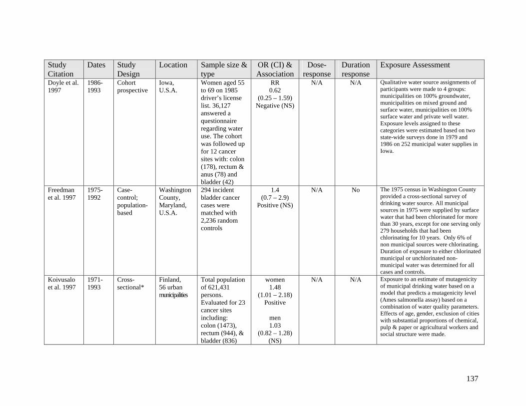
137

Study Citation

Dates Study Design

Location Sample size & type

OR (CI) & Association

Dose- response

Duration response

Exposure Assessment

Doyle et al. 1997

1986-1993

Cohort prospective

Iowa, U.S.A.

Women aged 55 to 69 on 1985 driver’s license list. 36,127 answered a questionnaire regarding water use. The cohort was followed up for 12 cancer sites with: colon (178), rectum & anus (78) and bladder (42)

RR 0.62

(0.25 – 1.59) Negative (NS)

N/A N/A Qualitative water source assignments of participants were made to 4 groups: municipalities on 100% groundwater, municipalities on mixed ground and surface water, municipalities on 100% surface water and private well water. Exposure levels assigned to these categories were estimated based on two state-wide surveys done in 1979 and 1986 on 252 municipal water supplies in Iowa.

Freedman et al. 1997

1975-1992

Case-control; population-based

Washington County, Maryland, U.S.A.

294 incident bladder cancer cases were matched with 2,236 random controls

1.4 (0.7 – 2.9)

Positive (NS)

N/A No The 1975 census in Washington County provided a cross-sectional survey of drinking water source. All municipal sources in 1975 were supplied by surface water that had been chlorinated for more than 30 years, except for one serving only 279 households that had been chlorinating for 10 years. Only 6% of non municipal sources were chlorinating. Duration of exposure to either chlorinated municipal or unchlorinated non-municipal water was determined for all cases and controls.

Koivusalo et al. 1997

1971-1993

Cross-sectional*

Finland, 56 urban municipalities

Total population of 621,431 persons. Evaluated for 23 cancer sites including: colon (1473), rectum (944), & bladder (836)

women 1.48

(1.01 – 2.18) Positive

men 1.03

(0.82 – 1.28) (NS)

N/A N/A Exposure to an estimate of mutagenicity of municipal drinking water based on a model that predicts a mutagenicity level (Ames salmonella assay) based on a combination of water quality parameters. Effects of age, gender, exclusion of cities with substantial proportions of chemical, pulp & paper or agricultural workers and social structure were made.

138

Study Citation

Dates Study Design

Location Sample size & type

OR (CI) & Association

Dose- response

Duration response

Exposure Assessment

King and Marrett 1996

Sep 1992 – May 1994

Case – control; population- based

Ontario, Canada

696 incident cases of bladder cancer with 1545 controls (matched for bladder, colon and rectal sites, the latter results reported in King et al. 2000)

1.6 (1.08 – 2.46)

Positive

yes yes A database was created for each drinking water supply including source (surface or groundwater) and chlorination status. A model was constructed to estimate THM level based on data from the Ontario Drinking Water Surveillance program (1986 – 1992) which was used to estimate THM levels from 1950 to 1990. Subjects were interviewed about water consumption 2 years prior and to provide water exposure history for at least 30 years. Exposure levels were assigned according to water source and modeled THM estimates for identified water sources.

Koivusalo et al. 1994

1967-1986

Aggregate Ecologic

56 Counties in Finland

32,551 incident cancer cases including: bladder (4144), colon (7233) and rectum (5253) used to calculate age-adjusted incident rates

N/A N/A N/A Exposure to an estimate of mutagenicity of municipal drinking water based on a model that predicts a mutagenicity level (Ames salmonella assay) based on a combination of water quality parameters. Assessments were made against water exposures classified as no mutagenicity, mutagenicity at less than 3000 revertants per L and for mutagenicity greater than 3000 revertants per L.

Suarez-Varela et al. 1994

1985-1989

Cross-sectional*; death certificates

Valencia and Valencia province, Spain

Population of 777,427 using chlorinated surface water; 1,230,500 using groundwater; bladder cancer cases based on death certificates

1.12 (0.85 – 1.49) Positive (NS)

no no Population using chlorinated surface water taken as exposed compared with population using groundwater as unexposed

139

Study Citation

Dates Study Design

Location Sample size & type

OR (CI) & Association

Dose- response

Duration response

Exposure Assessment

McGeehin et al. 1993

1988-1989

Case - control

Colorado, U.S.A.

327 incident bladder cancer cases with 261 other cancer site controls

1.8 (1.1 – 2.9) Positive

no yes 57 water utilities visited to abstract records on water source and disinfection. Data for THMs for 1989 used to determine an annual average used to represent historical water quality for systems without major changes over the period of 1926 to 1989. Residential location for each subject from age 20 were linked to water source as one of: chlorinated surface water, chloraminated surface water, chlorinated groundwater, non-chlorinated groundwater, bottled water and unknown.

Vena et al. 1993

1979-1985

Case – control; population-based

New York state, U.S.A.

351 white male incident bladder cancer cases with 855 white male population controls

2.98 (1.77 – 5.03)

Positive Males >65

yes no Fluid consumption was classified as tapwater vs. non-tapwater, but no assessment was made of the presence of disinfection byproducts in drinking water. Interviews provided various measures of fluid consumption that were linked for cases and controls.

Flaten 1992 1975-1984

Aggregate Ecologic

Norway Age adjusted cancer incidence rates were calculated for 15 cancer sites including bladder, colon and rectal cancer

N/A N/A N/A 96 municipalities (excluding Oslo) were categorized as chlorinated municipalities, non-chlorinating municipalities (no chlorinated water ever delivered) and partly chlorinating municipalities. Cancer incidence rates by municipality were compared with water supply category.

140

Study Citation

Dates Study Design

Location Sample size & type

OR (CI) & Association

Dose- response

Duration response

Exposure Assessment

Zierler et al. 1988

1978-1984

Case-control; population-based (death certificate)

Massachusetts, U.S.A.

614 bladder cases and 1074 controls for whom informants provided full responses satisfying exclusion criteria

1.4 (1.2 – 2.1) Positive

N/A yes Community water treatment systems were categorized as using chlorination or chloramination and subjects were classified according to duration of residence in chlorinated or a chloraminated water supplies with exposures classified as lifetime if residential water exposure was consistent since 1938 or “usual” if more than 50% of lifetime since 1938.

Cantor et al. 1987

Dec 1977- Dec 1978

Case – control; population-based

10 geographic regions, U.S.A.

2805 bladder cancer cases and 5258 controls provided sufficient information to classify by water source.

1.8 (NA)

Positive

NA N/A Survey of 1102 water utilities to determine water sources (surface or groundwater), treatment and distribution areas dating back to 1900. These data were geocoded in the same manner as the residential histories to allow linkage.

Zierler et al. 1986

1969-1983

Aggregate Ecologic

Massachusetts, U.S.A.

51,645 cancer deaths including: bladder (2311), colon (10,517), and rectum (2700) and 214,988 controls who died from non-cancer or lymphatic cancers.

1.05 (0.97 – 1.14)

NS

N/A N/A Community water treatment systems were categorized as using chlorination or chloramination and subjects were classified according to last residence before death as being either a chlorinated or a chloraminated water supply. Standardized incidence ratios for colon and rectum were compared by water source.

Isacson et al. 1983

1971-1980

Aggregate Ecologic

Iowa, U.S.A.

Cancer incidence data for 6 sites including bladder, colon and rectal cancer

N/A N/A N/A Drinking water source according to chlorination or no-chlorination

141

Study Citation

Dates Study Design

Location Sample size & type

OR (CI) & Association

Dose- response

Duration response

Exposure Assessment

Young and Kanarek 1983

1972-1977

Case-control, population-based, death certificate

28 counties, Wisconsin, U.S.A.

8,029 cancer deaths for 13 sites including bladder, colon and rectal cancer matched with 8029 non-cancer death controls

1.08 (N/A)

N/A N/A A reanalysis of data from Young and Kanarek 1981.

Kanarek and Young 1982

1972-1977

Case-control, population-based, death certificate

28 counties, Wisconsin, U.S.A.

Cancer deaths at 11 cancer sites including: colon (3184), rectum (778), and, bladder (458), for white women matched with an equal number of controls.

1.24 (N/A)

N/A N/A 202 water works were evaluated for a variety of characteristics and used in various treatment / exposure models, as well as a simple chlorinated – unchlorinated categorization to classify exposure according to the water works supplying the address reported on the death certificate.

Gottlieb and Carr 1982; Gottlieb et al. 1982

1960-1975

Case-control 13 counties, Louisana, U.S.A.

10,205 cancer deaths at 17 cancer sites (623 bladder cancer) were studied with 10,205 non-cancer death controls.

1.2 (N/A)

Positive (NS)

N/A yes Water supplies were classified as being surface or groundwater for the purpose of classifying each cancer death.

Bean et al. 1982

1969-1978

Aggregate Ecologic

Iowa, U.S.A.

Age-adjusted annual cancer incidence rates for sites including: bladder, colon, and rectal cancers

N/A N/A N/A Communities with a population >1000 and a public water supply that had been stable for >14 years were categorized by source of supply (surface or groundwater, including depth of well). Incidence rates by cancer site were analyzed in relation to water source.

142

Study Citation

Dates Study Design

Location Sample size & type

OR (CI) & Association

Dose- response

Duration response

Exposure Assessment

Wilkins and Comstock 1981

1963- 1975

Cohort, prospective

Washington County Maryland, U.S.A.

Cohort of 31,000 yielding 81 bladder cancer cases

Male 1.8

(0.8 -4.75) positive (NS)

Female

1.6 (0.54 – 6.32) positive (NS)

N/A N/A Drinking water exposure that were analyzed for association with causes of death were classified into 2 groups: Hagerstown residents (chlorinated surface water) and deep well users (non-chlorinated. A census had determined drinking water source by address for 98% of households, thereby allowing assignment of water exposure according to residential address.

Young et al. 1981

1972-1977

Case-control, population-based, death certificate

28 counties, Wisconsin, U.S.A.

8,029 cancer deaths for 13 sites including bladder, colon and rectal cancer) matched with 8029 non-cancer death controls

Female 1.04

(0.43 – 2.5) (NS)

no N/A Waterworks survey data in 1970 (based on data for 1960-1965) were used along with results from a questionnaire sent to waterworks superintendents to allow categorization of waterworks into high, medium and low chorine dosage. The residence listed on the death certificate for each case and control was used to assign a waterworks chlorine dose exposure.

Brenniman et al. 1980

1973-1976

Case-control, population-based, death certificates

Illinois, U.S.A.

3208 white cancer deaths for sites including: large intestine 1237, rectum 295 and bladder 284, with 43,666 control deaths.

0.98 (N/A)

negative (NS)

N/A N/A For a total of 542 communities using groundwater, 272 were chlorinated and 270 were non-chlorinated. Comparsions were made between these exposure categoriess.

Carlo and Mettlin 1980

1973-1976

Aggregate Ecologic

Erie County, New York, U.S.A.

4255 cases for sites including: colon, rectal, and bladder cancers were analyzed for incidence rates.

N/A N/A N/A THM4 was measured at water treatment plants in July 1978 (range 0 – 71 µg/L, mean 46 µg/L ). Correlation of the specified cancer incidence rates was determined with various demographic factors, water source type (surface – lake, river or reservoir or ground – well or spring).

143

Study Citation

Dates Study Design

Location Sample size & type

OR (CI) & Association

Dose- response

Duration response

Exposure Assessment

Cantor et al. 1978

1968-1971

Aggregate Ecologic

923 Counties (>50% urban) U.S.A.

Average annual age-adjusted mortality rates were calculated for 22 cancer sites including bladder, colon and rectal cancer.

N/A N/A N/A Chloroform and THM4 levels for major municipal water supplies were derived by a nation-wide survey conducted by the U.S. EPA in 1975 and a survey done in U.S. EPA Region V. Correlations were calculated between cancer mortality rates and THM4, chloroform or brominated THMs (by difference) for geographic regions where the majority of the water was provided by a sampled water supply.

Alavanja et al. 1978

1968-1970

Case-control, population-based, death certificates

7 Counties, New York State, U.S.A.

3446 gastrointestinal and urinary tract cancer deaths with 3444 matched controls

1.69 (N/A)

positive

N/A N/A Exposures were categorized as urban or rural, as well as for chlorinated vs. non-chlorinated and surface vs. groundwater sources using detailed water distribution maps to assign these exposures to geographic location for cases and controls.

Kuzma et al. 1977

1950-1969

Aggregate Ecologic

88 Counties, Ohio, U.S.A.

Age-adjusted cancer rates for 8 cancer sites including: large intestine, rectum, and bladder

N/A N/A N/A A U.S. Public Health Service inventory of water supplies in Ohio counties was used to assign exposure as being surface water or groundwater.

* exposure assessment in studies classified as cross-sectional are essentially ecological (not individual) in practice

144

Appendix A3 Reproductive Toxicology

145

Table A3-1 Reproductive Toxicology Studies on Chloroform by Ingestion or Intraperitoneal Injection Effects Species

Tested NOAEL (N)

or LOAEL (L) (for effect listed)

Dose Route, Range Tested & Duration

NOAEL or LOAEL as % of oral LD50a,b

Ratio of MAC to

NOAEL or LOAEL

Comments

Reference Citation

Fertility mouse N: 41 mg/kg-d gavage 0-41 mg/kg-d,

98 d

8.2 – 34% not applicable gavage

maternal toxicity Gulati et al. 1988

Sperm quality mouse N: 0.25 mg/kg-d IP injection 0 – 0.25 mg/kg-d

5 d

0.05 – 0.21% not applicable i.p. injection

some mortality Topham 1981

Fetotoxicity rat L: 200 mg/kg-d corn oil gavage 0 – 400 mg/kg-d

10 d

16 - 18% not applicable gavage

Fetotoxicity was ascribed to the 400 mg/kg-d dose level because the average fetus weight in this dose group was significantly depressed (19%) relative to the controls. Maternal weight gain was depressed and liver was enlarged in all exposure groups.

Ruddick et al. 1983

Embryotoxicity rat N: 126 mg/kg-d gavage 0 - 126 mg/kg-d

10d

9.8 – 12% not applicable gavage

maternal alopecia, rough appearance, reduced body weight gain

Thompson et al. 1974

Embryotoxicity rabbit L: 50 mg/kg-d gavage 0 - 50 mg/kg-d

13d

3.9 – 4.7% not applicable gavage

maternal anorexia, mild to severe diarrhea

Thompson et al. (1974)

Fetal development

rat L: 100 mg/kg-d gavage 0 – 400 mg/kg-d

10 d

7.8 – 9.4% not applicable gavage

Ruddick et al. (1983)

146

Effects Species Tested

NOAEL (N) or

LOAEL (L) (for effect listed)

Dose Route, Range Tested & Duration

NOAEL or LOAEL as % of oral LD50a,b

Ratio of MAC to

NOAEL or LOAEL

Comments

Reference Citation

Teratogenicity rat N: 126 mg/kg-d gavage 0 - 126 mg/kg-d

10d

9.8 – 12% not applicable gavage

maternal alopecia, rough appearance, reduced body weight gain

Thompson et al. (1974)

Teratogenicity rabbit N: 50 mg/kg-d gavage 0 - 50 mg/kg-d

13d

3.9 – 4.7% not applicable gavage

maternal anorexia, mild to severe diarrhea

Thompson et al. (1974)

Teratogenicity rat N: 400 mg/kg-d corn oil gavage 0 – 400 mg/kg-d

10 d

31– 38% not applicable gavage

No dose-related histopathological changes were observed in either mothers or fetuses at any level Maternal weight gain was depressed and liver was enlarged in all exposure groups. The overall conclusion was that chloroform is not teratogenic in the rat

Ruddick et al. (1983)

Teratogenicity mouse N: 855 mg/kg-d oral drinking water 0; 100; 1,000; 5,000 mg/L

56d

171-713% 50,000 No statistically significant teratologic effects in a two generation study. Ingestion at these levels produced significant decreases in body weight gain and livers showed pathology characteristic of chlorinated hydrocarbons

Borzelleca and Carchman 1982

a Oral LD50 for chloroform for female rats 1060 mg/kg-d (Thompson et al. 1974), and in corn oil 1117 (Chu et al. 1980) to 1280 mg/kg-d (Thompson et al. 1974). b Oral LD50 for chloroform for mice ranged from 120 to 500 mg/kg depending on strain (Hill et al. 1975)

147

Table A3-2 Reproductive Toxicology Studies on Chloroform by Inhalation Effects Species

Tested NOAEL (N)

or LOAEL (L)

(for effect listed)

Dose Route, Range

Tested & Duration

Ratio of NOAEL or LOAEL to

LC50a

Ratio of Equivalent MACb to

NOAEL or LOAEL

Comments

Reference Citation

Fertility rat L: 30 ppm (147 mg/m3)

inhalation 0 – 300 ppm, 6-15 d gest.

0.3% 147 for LOAEL

A conception rate of only 15% for rats exposed to 300 ppm was found

Schwetz et al. 1974

Sperm quality mouse L: 400 ppm (1960 mg/ m3)

inhalation 400 – 800 ppm

5 d

4.1% 1,960 for LOAEL

10 % mortality Land et al. 1981

Fetal toxicity rat L: 30 ppm (147 mg/m3)

inhalation 0 – 300 ppm, 6-15 d gest.

0.3% 147 for LOAEL

a high degree of fetal toxicity was observed at 100 and 300 ppm exposure that was not attributed to the observed maternal toxicity

Schwetz et al. (1974)

Fetal resorption

mice L: <100 ppm (<490 mg/m3)

inhalation 0, 100 ppm

1-7 d, 6-15 or 8-15d gestation

<1% <490 for LOAEL

maternal toxicity, significant increase in resorptions per litter during exposure days 1 to 7d of gestation

Murray et al. 1979

Embryotoxicity rat L: 30 ppm (147 mg/m3)

inhalation 0 – 300 ppm, 6-15 d gest.

0.3% 147 for LOAEL

a high degree of embryotoxicity was observed at 100 and 300 ppm exposure that was not attributed to the observed maternal toxicity

Schwetz et al. (1974)

Fetal development

mice L: <100 ppm (<490 mg/m3)

inhalation 0, 100 ppm

1-7 d, 6-15 or 8-15d gestation

<1% <490 for LOAEL

maternal toxicity, significant decrease in fetal body weight and crown-rump length for exposure 1-7d and 8-15d of gestation

Murray et al. 1979

Skeletal defects

mice L: <100 ppm (<490 mg/m3)

inhalation 0, 100 ppm

1-7 d, 6-15 or 8-15d gestation

<1% <490 for LOAEL

maternal toxicity, delayed ossification of skull bones

Murray et al. 1979

148

Effects Species Tested

NOAEL (N) or

LOAEL (L) (for effect listed)

Dose Route, Range

Tested & Duration

Ratio of NOAEL or LOAEL to

LC50a

Ratio of Equivalent MACb to

NOAEL or LOAEL

Comments

Reference Citation

Cleft palate mice L: <100 ppm (<490 mg/m3)

inhalation 0, 100 ppm

1-7 d, 6-15 or 8-15d gestation

<1% <490 for LOAEL

maternal toxicity, significantly more often for exposure at days 8-15 of gestation, but not for days 1-7 or 6-15.

Murray et al. 1979

Teratogenicity rat N: 30 ppm (147 mg/m3)

inhalation 0 – 300 ppm,

10 d

0.3% 1,470 for NOAEL

Observed a significant incidence of a number of developmental anomalies at 100 and 300 ppm. Chloroform was characterized as “not highly teratogenic”

Schwetz et al. (1974)

Teratogenicity rat N: 20,000 mg/m3

(4000 ppm)

inhalation 20,000 mg/m3

8 d

42% 4,000 for NOAEL

Abstract only. Increased fetal mortality and decreased fetal weight gain reported for sole dose tested

Dilley et al. 1977

a LC50 47,700 mg/m3 after Lundberg et al. 1986 b Shower air concentration of 1 mg/m3 estimated as equivalent to MAC of 100 µg/L based on experiments showing a median shower air to water partition ratio of 10 µg/m3 per µg/L.

149

Table A3-3 Reproductive Toxicology Studies on BDCM by Ingestion Effects Species

Tested NOAEL (N)

or LOAEL (L)

(for effect listed)

Dose Route, Range Tested & Duration

NOAEL or LOAEL as

% of oral LD50c

Ratio of NOAEL or

LOAEL conc. to MAC

Comments

Reference Citation

Reproductive rat N: 88 mg/kg-d (1300 mg/L)

oral / water 0 – 88 mg/Kg-d

9.3% 81,000 NTP 1998

Sperm quality rat F344

N: 22 mg/kg-d Oral / water 0 -39 mg/kg-d

56 weeks

2.3% not applicable gavage

Klinefelter et al. 1995

Sperm quality rat Sprague-Dawley

N: 69 mg/kg-da (450 mg/L)

oral / water 0-109 mg/kg-d

106d

7.3% 28,000 maternal mortality, reduced water consumption, reduced body weight and gains, reduced feed consumption, at 150 & 450 mg/L

Christian et al. 2002a

Fertility rat Sprague-Dawley

N: 69 mg/kg-da (450 mg/L)

oral / water 0-109 mg/kg-d

106d

7.3% 28,000 maternal mortality, reduced water consumption, reduced body weight and gains, reduced feed consumption, at 150 & 450 mg/L

Christian et al. (2002)

Fetal resorption rat F344

N: 25 mg/kg-d gavage 0-75 mg/kg-d

10d

2.7% not applicable gavage

Narotsky et al. 1997

Fetal resorption rat F344 & Sprague Dawley

N: 50 mg/kg-d gavage 0-100 mg/kg-d

5d

5.3% not applicable gavage

Found a dramatic difference in sensitivity between rat strains. F344 rats had 65% full-litter resorption at 75 mg/kg-d, SD had no effect up to 100 mg/kg-d

Bielmeier et al. 2001

Fetal resorption rat Sprague-Dawley

N: 82 mg/kg-d (900 mg/L)

oral / water 0-82 mg/kg-d 6-21 gest. d

8.7% 56,000 reduced maternal water consumption, body weight gain and feed consumption at 45 mg/kg-d

Christian et al. 2001

150

Effects Species Tested

NOAEL (N) or

LOAEL (L) (for effect listed)

Dose Route, Range Tested & Duration

NOAEL or LOAEL as

% of oral LD50c

Ratio of NOAEL or

LOAEL conc. to MAC

Comments

Reference Citation

Fetal resorption rabbit N: 55 mg/kg-d (900 mg/L)

oral / water 0-55 mg/kg-d 6-29 gest. d

≥ 5.8% 56,000 reduced maternal water consumption, body weight gain and feed consumption at 35.6 mg/kg-d (55.3 mg/kg-d for weight loss)

Christian et al. (2001)

Fetal resorption rat F344

L: 75 mg/kg-d gavage 0 - 75 mg/kg-d 6 – 10 gest. d

8% not applicable gavage

Fetal resorption at 10d was associated with marked reduction in serum progesterone and lutenizing hormone. Progesterone replacement even at BDCM dosed at 100 mg/kg-d prevented fetal resorption

Bielmeier et al. 2004

Fetal resorption rat F344

Not applicable gavage 0 - 100 mg/kg-d

6 – 9 gest. d

Not applicable not applicable gavage

Dams sacrificed at gestational day 9 after exposure to BDCM at 100 mg/kg-d showed in vitro corpus luteum secretion of progesterone >2 fold higher than controls, contrary to hypothesis of BDCM reducing progesterone secretion as mechanism for fetal resorption

Bielmeier et al. 2007

Fetotoxicity rat N: 200 mg/kg-d gavage 0-200 mg/kg-d

10d

21% not applicable gavage

Ruddick et al. (1983)

Fetotoxicity rat F344

N: 75 mg/kg-d gavage 0-75 mg/kg-d

10d

8% not applicable gavage

Narotsky et al. (1997)

151

Effects Species Tested

NOAEL (N) or

LOAEL (L) (for effect listed)

Dose Route, Range Tested & Duration

NOAEL or LOAEL as

% of oral LD50c

Ratio of NOAEL or

LOAEL conc. to MAC

Comments

Reference Citation

Fetotoxicity rat Sprague-Dawley

N: 45 mg/kg-d (450 mg/L)

oral / water 0-82 mg/kg-d 6-21 gest. d

4.8% 28,000 reduced maternal water consumption, body weight gain and feed consumption at 45 mg/kg-d

Christian et al. (2001)

Fetotoxicity rabbit N: ≥ 55 mg/kg-d (≥ 900 mg/L)

oral / water 0-55 mg/kg-d 6-29 gest. d

≥ 5.8% 56,000 reduced maternal water consumption, body weight gain and feed consumption at 35.6 mg/kg-d (55.3 mg/kg-d for weight loss)

Christian et al. (2001)

Gestation length rat F344

N: 75 mg/kg-d gavage 0-75 mg/kg-d

10d

8% not applicable gavage

Narotsky et al. (1997)

Gestation length rat Sprague-Dawley

N: 69 mg/kg-da (450 mg/L)

oral / water 0-109 mg/kg-d

106d

7.3% 28,000 maternal mortality, reduced water consumption, reduced body weight and gains, reduced feed consumption, at 150 & 450 mg/L

Christian et al. (2002)

Fetal weight rat N: 200 mg/kg-d gavage 0-200 mg/kg-d

10d

21% not applicable gavage

Ruddick et al. (1983)

Fetal weight rat F344

N: 75 mg/kg-d gavage 0-75 mg/kg-d

10d

8% not applicable gavage

Narotsky et al. (1997)

Fetal weight rat Sprague-Dawley

N: 45 mg/kg-d (450 mg/L)

oral / water 0-82 mg/kg-d 6-21 gest. d

4.8% 28,000 reduced maternal water consumption, body weight gain and feed consumption at 45 mg/kg-d

Christian et al. (2001)

Fetal weight rabbit N: ≥ 55 mg/kg-d (≥ 900 mg/L)

oral / water 0-55 mg/kg-d 6-29 gest. d

≥ 5.8% 56,000 reduced maternal water consumption, body weight gain and feed consumption at 35.6 mg/kg-d (55.3 mg/kg-d for weight loss)

Christian et al. (2001)

152

Effects Species Tested

NOAEL (N) or

LOAEL (L) (for effect listed)

Dose Route, Range Tested & Duration

NOAEL or LOAEL as

% of oral LD50c

Ratio of NOAEL or

LOAEL conc. to MAC

Comments

Reference Citation

Postnatal survival

rat F344

N: 75 mg/kg-d gavage 0-75 mg/kg-d

10d

8% not applicable gavage

Narotsky et al. (1997)

Embryotoxicity rat F344

Effects seen at only dose level

tested

gavage 75 mg/kg-d

2-10d

- not applicable gavage

Narotsky et al. (1997)

Teratogenicity rat N: 200 mg/kg-d gavage 0-200 mg/kg-d

10d

21% not applicable gavage

Ruddick et al. (1983)

Delayed sexual maturation

rat Sprague-Dawley

N: 26 mg/kg-da (150 mg/L)

oral / water 0-109 mg/kg-d

106d

7.3% 9,400 maternal mortality, reduced water consumption, reduced body weight and gains, reduced feed consumption, at 150 & 450 mg/L

Christian et al. (2002)

Reproductive organs / placenta

human placental

trophoblasts in vitro

L: 3.3 µg/L in vitro culture 0 – 330 mg/L

1 d

Not applicable because of

in vitro experiment

Not applicable because of

in vitro experiment

The lowest BDCM dose for effect on chorionic gonadotrophin secretion was approximately 35 times higher than the maximum human blood BDCM concentration measured after showering

Chen et al. 2003

Reproductive organs / placenta

human placental

trophoblasts in vitro

N: 3.3 mg/L in vitro culture 0 – 330 mg/L

1 d

Not applicable because of

in vitro experiment

Not applicable because of

in vitro experiment

The lowest BDCM dose for effect on disruption of trophoblast differentiation (33 mg/L) was approximately 350,000 times higher than the maximum human blood BDCM concentration measured after showering

Chen et al. 2004

153

Effects Species Tested

NOAEL (N) or

LOAEL (L) (for effect listed)

Dose Route, Range Tested & Duration

NOAEL or LOAEL as

% of oral LD50c

Ratio of NOAEL or

LOAEL conc. to MAC

Comments

Reference Citation

Skeletal defects rat Sprague-Dawley

N: 45 mg/kg-db (450 mg/L)

oral / water 0-82 mg/kg-d 6-21 gest. d

4.8% 28,000 reduced maternal water consumption, body weight gain and feed consumption at 45 mg/kg-d

Christian et al. (2001)

a median of consumption doses estimated for specified BDCM exposure concentrations, Christian et al. (2002) b mean of consumption doses for specified BDCM exposure concentrations, Christian et al. (2001) c rat oral LD50 median = 943 (916 – 969) mg/kg-d Chu et al. (1980)

154

Table A3-4 Reproductive Toxicology Studies on Haloacetic Acids Effects DBP Species

Tested NOAEL (N)

or LOAEL (L)

(for effect listed)

Dose Route, Range Tested & Duration

NOAEL or LOAEL as

% of oral LD50

Ratio of NOAEL or

LOAEL conc. to MAC

Comments

Reference Citation

Sperm quantity and quality

DCAA rat male

Long-Evans

L: 31.25 mg/kg-d

oral gavage 0 -125 mg/kg-d

10 weeks

0.63%a not applicable gavage

reduced epididymal sperm counts and sperm motility and impacted sperm morphology at lowest doses

Toth et al. 1992

Sperm quantity and quality

DCAA rat male

Sprague-Dawley

N: 54 mg/kg-d oral gavage 0 -1,440 mg/kg-d

14 days

0.63%a not applicable gavage

decreased epididymal sperm count and increased abnormalities at 160 mg/kg-d

Linder et al. 1997

Sperm quantity and quality

DBAA rat male

Sprague-Dawley

L: 1250 mg/kg oral gavage single dose 1250 mg/kg

28 days observation

64-89%b not applicable gavage

sperm motility reduced and morphology affected 14 and 28 days after dosing

Linder et al. 1994

Sperm quantity and quality

MBAA rat male

Sprague-Dawley

N: 25 mg/kg-d oral gavage 25 mg/kg 14 days

11-16%c not applicable gavage

no reproductive related end-points observed

Linder et al. (1994)

Fetal Resorption DCAA rat Long-Evans

N: 14 mg/kg-d oral gavage 0-2,400 mg/kg-d

0.28% not applicable gavage

significant elevation of resorbed implants at ≥900 mg/kg-d. 7 maternal deaths at doses >1,400 mg/kg-d and maternal weight loss at >14 mg/kg-d

Smith et al. 1992

155

Effects DBP Species Tested

NOAEL (N) or

LOAEL (L) (for effect listed)

Dose Route, Range Tested & Duration

NOAEL or LOAEL as

% of oral LD50

Ratio of NOAEL or

LOAEL conc. to MAC

Comments

Reference Citation

Fetal weight DCAA rat Long-Evans

N: 14 mg/kg-d oral gavage 0-2,400 mg/kg-d

0.28% not applicable gavage

Dose dependent reduction in live fetal weight for doses > 140 mg/kg-d. 7 maternal deaths at doses >1,400 mg/kg-d and maternal weight loss at >14 mg/kg-d

Smith et al. (1992)

Soft tissue malformations (mainly cardiovascular system)

DCAA rat Long-Evans

N: 14 mg/kg-d oral gavage 0-1,800 mg/kg-d

0.28% not applicable gavage

Significant increase (2.6%) at 140 mg/kg to 73% at 2,400 mg/kg-d. 7 maternal deaths at doses >1,400 mg/kg-d and maternal weight loss at >14 mg/kg-d

Smith et al. (1992)

Fetal Resorption TCAA rat Long-Evans

L: 330 mg/kg-d oral gavage 0-1,800 mg/kg-d

6.6% not applicable gavage

significant elevation of resorbed implants at ≥800 mg/kg-d.

Smith et al. 1989

Fetal weight TCAA rat Long-Evans

L: 330 mg/kg-d oral gavage 0-1,800 mg/kg-d

6.6% not applicable gavage

Dose dependent reduction in live fetal weight at all doses tested

Smith et al. (1989)

Soft tissue malformations (mainly cardiovascular system)

TCAA rat Long-Evans

L: 330 mg/kg-d oral gavage 0-1,800 mg/kg-d

6.6% not applicable gavage

Significant increase (9%) at 330 mg/kg to 97% at 1,800 mg/kg-d

Smith et al. (1989)

156

Effects DBP Species Tested

NOAEL (N) or

LOAEL (L) (for effect listed)

Dose Route, Range Tested & Duration

NOAEL or LOAEL as

% of oral LD50

Ratio of NOAEL or

LOAEL conc. to MAC

Comments

Reference Citation

Skeletal malformations

TCAA rat Long-Evans

N: 800 mg/kg-d oral gavage 0-1,800 mg/kg-d

16% not applicable gavage

mainly in the small orbit at doses ≥1200 mg/kg-d

Smith et al. (1989)

Reproductive tract malformations

DBAA rat 50 mg/L (4.5 – 11.6 mg/kg-d)

oral drinking water 50, 250, 650

mg/L (4.4-11.6, 22.4-55.6, 52.4 – 132

mg/kg-d)

0.23-0.8% >833 Authors note that the NOAEL was 45,000 to 116,000 human adult exposure levels and concluded that DBAA should not be considered as a human reproductive or developmental risk.

Christian et al. 2002b

a dichloroacetic acid (DCAA) rodent oral LD50 = 5000 mg/kg-d (Stacpoole et al. 1998) b dibromoacetic acid (DBAA) rat oral LD50 = 1737 (1411 – 1952) mg/kg (Linder et al. 1994) c monobromoacetic acid (MBAA) rat oral LD50 = 177 (156 – 226) mg/kg (Linder et al. 1994)

157

Appendix A4 Adverse Reproductive Effects Epidemiology

158

Table A4-1 Epidemiology Studies on Adverse Reproductive Outcomes Reference Dates Study

Design Location Sample size Outcomes Exposure Assessment

Nieuwenhuijsen et al. 2008

1993 - 2001

Retrospective Cohort (Cross – sectional)

England and Wales – 12 water companies serving 44 million consumers

2,605,226 live births

AbWl (2,267) ClDef (3,736) McdAn (8,809) NTDef (3,334) RsDef (1,434) UrTrDef (5,315)

A weighted average modeled quarterly THM estimate for each water zone was linked to postal code for maternal residence at time of birth for each birth record. THM4 were categorized as THM4 <30 µg/L, 30 to <60 µg/L and ≥60 µg/L, total brominated THMs <10 µg/L, 10 to <20 µg/L and ≥20 µg/L, and bromoform <2 µg/L, 2 to <4 µg/L and ≥4 µg/L,

Hwang et al. 2008

2001 - 2003

Retrospective Cohort (Cross – sectional)

Taiwan 396,049 births (325,240 births excluded because of insufficient water disinfection information)

Anen (43) Bdef (2,148) ChAb (364) DnSyn (166) Hyceph (118) Hyp 72 RenDef (76) UrTrDef (49) VSDef (59)

The Taiwanese Water Supply Corporation has 200 water treatment plants serving 21 million consumers. One or more water treatment plant serve each municipality so levels of THM4 for each water treatment plant were linked with mother’s place of residence during pregnancy to classify exposure to THM4 as high: >20 µg/L, medium: 10 – 19 µg/L, low 5 – 9 µg/L compared to lowest 0 – 4 µg/L

Chisholm et al. 2008

2000 - 2004

Retrospective Cohort (Cross – sectional)

Perth metropolitan region, Australia

20,874 live births BDef (1097) CdAn (260) CNSAn (59)

THM samples collected on 6 occasions from 47 sites that were grouped into 3 zones described as low, medium and high THM. Exposure was assigned based on postal code of maternal residence at time of birth

159

Reference Dates Study Design

Location Sample size Outcomes Exposure Assessment

Yang et al. 2007

2000-2002

Retrospective Cohort (Cross – sectional)

Taiwan 90,848 women in 65 municipalities with a first parity singleton birth for which complete information available.

term LBWt (2766) PTm (2818) SGA (8938)

THM4 was used as a marker for chlorination by-product exposure based on quarterly sampling over 2 years from each of 65 municipalities. Exposure was assigned based on average THM4 for the municipality of maternal residence at birth assuming that the mother listed on the birth certificate lived at that residence throughout the pregnancy.

Toledano et al. 2005

1992 - 1998

Retrospective Cohort (Cross – sectional)

England Northumbrian, United Utilities and Severn Trent water service areas

920,571 live and still births (including 869,314 live birth allowing birth weight analysis)

StBth (4852) LBWt (60641) VLBWt (9167)

Variable THM monitoring data (1 to 80 measurements per year depending on compliance level) were used to model THM4 levels per regional zone. Postal code of maternal residence was used to assign an exposure zone and THM4 exposure was estimated for the 3rd trimester.

Savitz et al. 2005; Savitz et al. 2006

Dec 2000 to Apr 2004

Prospective cohort

Texas, North Carolina and Tennessee, U.S.A.

3132 women recruited in early pregnancy (including 252 prior to conception), with 2,409 women retained for data analysis

SpAb (258) PTm (196) SGA (102)

Weekly distribution system samples (reduced to bi-weekly at low DBP site) for confirmed spatially homogenous systems monitored for THM4, HAA9 and TOX. Various exposure indices evaluate for enrolled women, including average of weekly DBP concentration over the duration of pregnancy. Interviews at recruitment and at 20-25 wks gestation to evaluate water uses and other risk factors.

Porter et al. 2005

1998 - 2002

Retrospective Cohort (Cross – sectional)

Maryland, U.S.A. 4 regions of one county

15,315 singleton births with race recorded

IUGR (1114) Bi-weekly averaged THM4 and HAA5 routine monitoring data were determined for each region and matched to maternal residence in a region and estimated gestational period for each pregnancy

160

Reference Dates Study Design

Location Sample size Outcomes Exposure Assessment

Hinckley et al. 2005

Jan 1998 to Mar 2003

Retrospective Cohort (Cross – sectional)

Arizona, U.S.A. 3 water treatment facilities in a community of approx. 500,000

48,119 (live births and fetal deaths)

IUGR (4,346) term LBWt (1,010) PTm (4,008) very PTm (564)

Quarterly THM and HAA (as available) from community system regulatory monitoring were assigned to maternal ZIP code and applied to corresponding exposure windows for various birth outcomes evaluated.

King et al. 2005 1999 - 2001

Retrospective Cohort (Cross – sectional)

Eastern Ontario and Nova Scotia, Canada

398 live birth controls

StBth (112) Residential water samples 1 year later to estimate at 3 – 4 month gestation for total HAA and dichloroacetic acid plus interviews to estimate work exposures and determine water use behaviours

Wright et al. 2004

1995 - 1998

Retrospective Cohort (Cross – sectional)

Massachusetts, U.S.A.

196,000 live birth certificates

PTm (11,580 ) 109 communities > 10,000 provided routine quarterly (9 had only annual) routine THM monitoring data for 1995 – 1998. 17 communities collected HAA data (weekly or quarterly) in 1997-1998. MX and mutagenicity were data collected in 88 tap water samples from 36 communities in 1997-1998. Maternal ZIP code and infant month of birth were used to assign DBP values approximating 3rd trimester exposure based on community monitoring data.

Yang 2004 1994-1996

Retrospective Cohort (Cross – sectional)

Taiwan 182,796 women with first parity singleton

LBWt (8251) PTm (80,030)

The study population was located in either 113 chlorinating municipalities (>95% served by chlorinated water) or 15 non-chlorinating municipalities (<5% served by chlorinated water) among 310 municipalities studied.

161

Reference Dates Study Design

Location Sample size Outcomes Exposure Assessment

Infante-Rivard 2004

1998 - 2000

Case control Québec, Canada 493 cases 472 normal weight controls

IUGR (493) THM levels estimated from routine regulatory monitoring data for the treatment plant serving the maternal residence and in-person interviews determined water use behaviour and consumption

Dodds et al. 2004

1999 - 2001

Retrospective Cohort (Cross – sectional)

Eastern Ontario and Nova Scotia, Canada

398 live birth controls

StBth (112) Residential water samples 1 year later to estimate at 3 – 4 month gestation plus interviews to estimate work and other THM exposures and determine water use behaviours for dermal and inhalation exposures

Aggazzotti et al. 2004

Oct 1999 – Sep 2000

Prospective cohort

Italy 9 cities

1194 live births PTm (343) SGA (239)

Water samples collected at each women’s home within a few days of delivery and analyzed for individual THMs (n=1194) and for chlorite and chlorate where chlorine dioxide was used alone or in combination with chlorine (n=893). Individual questionnaires addressed consumption and habits

Wright et al. 2003

1990 Retrospective Cohort (Cross – sectional)

Massachusetts, U.S.A. 96 communities larger than 10,000, most with quarterly THM data

56,513 live births term LBWt (1325) SGA (5310) PTm (3173)

Town average quarterly THM data for 3rd trimester matched to maternal address. Some missing THM data imputed from other years

Windham et al. 2003

1990 - 1991

Prospective cohort

California, U.S.A. 402 pre-menopausal women

Daily urine samples from each woman over and average of 5.6 menstrual cycles from a prospective study of menstrual cycle function was analyzed with estimates of THM exposure according to Waller et al. (1998) including interiews concerning water consumption

162

Reference Dates Study Design

Location Sample size Outcomes Exposure Assessment

Shaw et al. 2003

1987 - 1991

Retrospective Cohort (Cross – sectional)

California, U.S.A. Study 1: 1077 live births Study 2: 1362 live births

Study 1: NTDef (538) Study 2 NTDef (265) CdAn (207) OfC (409)

Water utility averages from quarterly THM monitoring matched to maternal address. Interviews to estimate tap water consumption

Hwang et al. 2002

1993 - 1998

Retrospective Cohort (Cross – sectional)

Norway 1317 water works with data on colour and chlorination

184,676 births BDef (5764) including: NTDef (138) MCdAn (537) RsDef (192) UrTrDef (232) 343 (OC)

Mean colour for waterworks and proportion served by chlorination calculated for each municipality and mother’s municipality at time of birth matched to waterworks using 1994 registry. Extension of Magnus et al. (1999) to add 1996 to 1998.

Cedergren et al. 2002

1982 - 1986

Retrospective Cohort (Cross – sectional)

Sweden 80 water supplies in one county

71,978 live births that allowed assignment of geocode to mother

753 CdAn Data from water suppliers on chlorination or chlorine dioxide disinfection practices along with limited THM data from one year were used to estimate exposures by GIS overlay with maternal geocode.

Waller et al. 2001b

1989 - 1991

Prospective cohort (re-analysis)

California, U.S.A. 3 regions served by 85 water utilities

4212 pregnancies SpAB (~400) Quarterly municipal water surveys to estimate average THM for 1st trimester based on maternal residence. Telephone interview to estimate tap water consumption at 8 wks gestation. Reanalysis of Waller et al. (1998) comparing two methods of THM exposure classification

Jaakkola et al. 2001

1993 - 1995

Retrospective Cohort (Cross – sectional)

Norway 1317 water works with data on colour and chlorination

137,145 live births LBWt (6249) PTm (7886)

Colour(high or low) for waterworks and chlorination (yes or no) used to determine 4 exposure categories for mother’s municipality at time of birth matched to waterworks using 1994 registry. Same population as Magnus et al. (1999), but analysis for different birth outcomes

163

Reference Dates Study Design

Location Sample size Outcomes Exposure Assessment

Dodds and King 2001

1988 - 1995

Retrospective Cohort (Cross – sectional)

Nova Scotia, Canada 49,842 live and StBth

NTDef (77) OCf (82) MCdAn (430) ChAb (96)

THM4 levels estimated with linear regression using measurements from 3 locations in distribution system sampled 4 times per yr (irregular intervals) matched to maternal address at delivery. Analysis done for chloroform and BDCM exposure not THM4

Kallen and Robert 2000

1985- 1994

Retrospective Cohort (Cross – sectional)

Sweden Compared liquid chlorine, chlorine dioxide and no disinfection

singleton deliveries 24,731 (liquid chlorine) 15,429 (chlorine dioxide) 74,324 (no disinfection)

PTm LBWt VLBWt SGA CdAn ClDef

Maternal location in area according to disinfection method (liquid chlorine, chlorine dioxide or none) for 1985, 1989 and 1994.

Yang et al. 2000

1994-1996

Retrospective Cohort (Cross – sectional)

Taiwan 14 municipalities using unchlorinated groundwater matched to 14 municipalities using chlorinated surface water

18,025 first parity, singleton live births

PTm (719) term LBWt (456)

Municipalities were either >90% or <5% of population served by chlorinated water. Used maternal address at delivery to determine municipality.

King et al. 2000a

1988-1995

Retrospective Cohort (Cross – sectional)

Nova Scotia, Canada 49,756 singleton deliveries

StBth (214) including: 72 asphyxia, 20 immaturity, 15 CAn, 2 infection, 21 other specified causes and 84 unexplained)

THM4 levels estimated with linear regression using measurements from locations in distribution system generally sampled 4 times per yr (irregular intervals) matched to maternal address at delivery.

164

Reference Dates Study Design

Location Sample size Outcomes Exposure Assessment

Magnus et al. 1999

1993-1995

Retrospective Cohort (Cross – sectional)

Norway Municipalities with data on chlorination and colour

141,077 total births

BDef (2608) including: NTDef (62) MCdAn (250) RsDef (91) UrTrDef (122) OC (143)

Mean colour for waterworks and proportion served by chlorination calculated for each municipality and mother’s municipality at time of birth matched to waterworks using 1994 registry.

Dodds et al. 1999

1988 - 1995

Retrospective Cohort (Cross – sectional)

Nova Scotia, Canada 49,842 singleton deliveries

NTDef (77) OCf, (82) MCdAn (430) ChAb (96) SmGA (4673) LBWt (2392) VLBWt (342) PTm (2689) StBth (197) ChAb (96)

THM4 levels estimated with linerar regression using measurements from 3 locations in distribution system sampled 4 times per yr (irregular intervals) matched to maternal address at delivery.

Waller et al. 1998

1989 - 1991

Prospective cohort

California, U.S.A. 3 regions served by 85 water utilities

5144 pregnancies SpAB (~500) Quarterly municipal water surveys to estimate average THM for 1st trimester based on maternal residence. Telephone interview to estimate tap water consumption at 8 wks gestation

Klotz and Pyrch 1999

1993 - 1994

Case control; population - based

New Jersey, U.S.A. drawn from total (approx. 250,000 births)

112 cases and 248 controls (full term, ≥2500 g, no other defects)

NTDef (112) Municipal water surveys for maternal address and tap water sampling 1 yr after critical effect (i.e. 4 mth age if full term delivery)

Gallagher et al. 1998

1990 - 1993

Retrospective Cohort (Cross – sectional)

Colorado, U.S.A., 2 water districts near Denver

1244 singleton, white births at 28-42 wks

LBWt (72) term LBWt, (29) PTm (68)

Municipal water samples in 3rd trimester matched to mother’ residence at time of birth. Hydraulic modeling estimate of household THM4 level for 3rd trimester

165

Reference Dates Study Design

Location Sample size Outcomes Exposure Assessment

Kanitz et al. 1996

1988 - 1989

Retrospective Cohort (Cross – sectional)

Liguria, Italy; 2 hospitals (Genoa and Chiavari)

548 LBth in Genoa and 128 in Chiavari

PTm (50), LBW (20) SmBL (288) SmCrC (370) NnJd (133)

Maternal address used to determine water source type (chlorine dioxide, liquid chlorine, or both vs. not treated)

Savitz et al. 1995

Sep 1988 – Aug 1989 or 1991

Case – control; population - based

North Carolina, U.S.A. 1 county and 6 area hospitals

548 cases 455 controls

PTm (244) LBW (178) SpAB (126)

Maternal address and pregnancy date used to assign a quarterly average THM4 level from 1 of 5 water supplies. MsCg cases and controls used date closest to 4th wk gestation. PTm and LBWt cases and controls used date closest to 28th wk gestation

Bove et al. 1995

1985 - 1988

Retrospective Cohort (Cross – sectional)

New Jersey, U.S.A.; 75 towns in northern New Jersey counties, some water supplies contaminated with solvents

81,532 total 80938 live births comparison group of 52,334 not LBW, not SmGA not PTm and no defects)

BDef (669) CNSAn(118) NTDef (56) OCf 83) CdAn (346) MCdAn (108) VSDef (87) term LBWt (1853) VLBWt (905) SGA (4082) PTm (7167) FDth (594)

Study directed at solvent contamination but maternal address and 4 or more municipal water samples per quarter were used to estimate monthly THM4. First trimester used for birth defects and fetal death; 9 month levels for other outcomes.

Aschengrau et al. 1993

Aug 1977 – Mar 1980

Case – control; hospital - based

Massachusetts, U.S.A.

2348 total 1177 controls

CAn (1039) StBth (77) NnDth (55)

Maternal address & routine municipal water sample. Treated surface water vs. untreated ground / mixed water. Chlorination vs. chloramination for surface water

Kramer et al. 1992

Jan 1989 – Jun 1990

Case – control; population - based

Iowa, U.S.A., 151 towns of 1000 to 5000 with single water source

4128 total: 688 cases

PTm (342), LBWt (159) SGA (187)

Maternal address at time of birth with THM levels of towns using special municipal water survey (drought)

166

Reference Dates Study Design

Location Sample size Outcomes Exposure Assessment

Aschengrau et al. 1989

Jul 1976 – Feb 1978

Case – control hospital - based

Massachusetts, U.S.A.

1677 total; 286 cases; 1391 controls (live born, ≥37 wk)

SpAb through 27 weeks

Maternal address & routine municipal water sample. Treated surface water vs. untreated ground / mixed water. Chlorination vs. chloramination for surface water

167