a practical method for determination of economic

Journal of Thermal Engineering, Vol. 6, No. 1, pp. 72-86, January, 2020 Yildiz Technical University Press, Istanbul, Turkey

This paper was recommended for publication in revised form by Regional Editor Mustafa Kılıc

1Department of Mechanical Engineering, Yildiz Technical University, Istanbul, TURKEY 2M.Sc. Energy Conversion and Management, Istanbul, TURKEY *E-mail address: [email protected] Orcid id: 0000-0002-0450-4818, 0000-0001-7895-4478 Manuscript Received 27 February 2018, Accepted 18 May 2018

A PRACTICAL METHOD FOR DETERMINATION OF ECONOMIC INSULATION THICKNESS OF STEEL, PLASTIC AND COPPER HOT WATER PIPES

N. Alpay Kürekci1,*, Mehmet Özcan2

ABSTRACT

Hot water systems are being extensively used in residential as well as industrial contexts. Choice of insulation material’s thickness has a significant effect on total cost. The purpose of this study was to develop a simplified but accurate empirical method that allows to determine the optimum thicknesses of the insulation materials that are applied on the hot water pipes. In the first step, a comprehensive mathematical model was constructed for the calibration and validation purposes. Then, the heat transfer between the flow inside the pipe and the external environment was thermally modeled; followed by a calculation of fuel and insulation costs. After that, the total cost analysis method was applied in order to define the optimum insulation thickness. Later an empirical method was developed based on the mathematical model. Finally, the accuracy of the empirical method was tested, using a wide range of physical conditions as well as different insulation materials, pipe and fuel types. The standard optimum insulation thickness values were founded same for the all pipe types with the identical diameters. The heat losses can be reduced around 89, 88 and 83% by application of optimum insulation thickness to steel, copper and plastic pipes respectively. Larger pipes have higher net savings and lower payback periods. Fuel-oil is the least economic heating solution; therefore the application of insulation brings higher profits than the other fuels. Prediction accuracy of the empirical method is higher for the steel and copper pipes than the plastic pipes. An average matching rate of 91.4% indicated that the new method is a valid and time-saving alternative, which can be used in pipe insulation applications. Keywords: Heat Transfer Pipes, Optimum Insulation Thickness, Energy Saving, Thermo-Economic Analysis, Mathematical Modeling, Thermal Insulation

INTRODUCTION

Various socioeconomic causes such as population growth, industrialization and increase in energy consumption per capita lead to a steady increase in global primary energy consumption. Between the years 2010 and 2014, energy supply and demand growth were accounted as 5.12% and 8.62% respectively [1]. In 2016, only 3.16% of the world's primary energy, excluding hydropower, was supplied from renewable energy sources [2]. Due to steady increase in energy prices, the prevailing share of non-renewable energy sources on total energy demand and limited energy resources, energy efficiency is becoming a topic of increasing importance. Among various energy saving measures, thermal insulation is known as one of the most cost-effective ways to improve energy efficiency [3] - as long as suitable insulation materials are used and a balance point between the cost and the energy savings is obtained [4].

Today, especially in residential buildings, heating networks are either not equipped with thermal insulation, or only cheap and thin materials are used in order to keep the initial investment cost as low as possible. Heat losses reduce energy efficiency, thus leading to increased operational costs and carbon emissions. They also cause an increase in the heating system capacity and thereby in the investment cost [5].

Various studies have been carried out in order to define the optimum thermal insulation thickness of pipes. Zhang, L. et al. [4] thermo-economically analyzed the optimum insulation thickness for buried pipes of district heating systems and investigated the impacts of various pipe diameters, fuel types and soil depths on energy savings and payback periods.

Daşdemir A. et al. [6] investigated the optimum insulation thickness of pipes used in HVAC pipe applications. They built an optimization model based on thermal equations and Life Cycle Cost (LCC) analysis via P1-P2 method, which simplifies the economic analysis by categorizing the total lifecycle savings and expenses. The model was used for determination of the annual total cost, energy saving and payback periods of various

mailto:[email protected]

Journal of Thermal Engineering, Research Article, Vol. 6, No. 1, pp. 72-86, January, 2020

73

insulation scenarios. Various diameters of steel, plastic and copper pipes, as well as three insulation materials and fuel types were used to generate different scenarios.

Öztürk I. et al. [7] presented four different thermo-economic techniques for optimum design of hot water pipe systems. Such techniques were based on optimization of pipe diameters and insulation thicknesses by taking the total cost, heat losses and exergy efficiencies into account.

Açıkkalp E. et al. [8] used a novel method, which was based on a combination of exergy and environmental analyses, to determine the optimum insulation thickness for a piping system. They investigated the net savings of the environmental impact and exergetic heat loss, as well as fuel consumption and CO2 emissions for insulation application on DN50, DN100 and DN150 stainless steel pipes.

A considerable amount of research has been conducted on examination of different scenarios of heat losses, savings and costs of pipe insulations. Highly informative and useful graphs and tables were presented in order to help readers with the determination of the optimum insulation thickness for various fuel types, insulation materials, and pipe diameters. Nevertheless, the scope of those studies has been limited to specific countries and cities. Moreover, interest and inflation rates, fuel and insulation prices have been defined according to the economic conditions of the day and the region [6-10].

The aim of this study is to present a practical but yet an accurate method for the calculation of economic insulation thickness. The following objectives are addressed: First, a comprehensive mathematical model is explained. Then the simplified empirical method is proposed. After that, the effects of various conditions on economic insulation thickness, energy saving and payback period are compared. Later, a sensitivity analysis of DN50 pipe is conducted to compare the effects of various parameters on economic insulation thickness. Finally, the accuracy of the heat loss correlations and simplified method are presented. The proposed new method has an acceptable accuracy, brings the parametric flexibility and can be quickly conducted to a wide range of physical and economic conditions. Therefore, it will constitute an important place both in the scientific and practical fields.

DESCRIPTION OF SYSTEM AND MATHEMATICAL MODEL

The analyzed system is a hot water pipe covered with thermal insulation and exposed to ambient air. The aluminum cover on the insulation material was assumed to be thin and thermally highly conductive; therefore, its conduction resistance was neglected in heat transfer calculations. Nevertheless, radiation heat transfer from the external surface was taken into account. Water and air were defined as internal and external fluid domains respectively. The thermal properties of water, air, pipe and insulation materials were determined with respect to the individual temperatures of the mediums. The model of the pipe section is shown in Figure 1.

Figure 1. Schematic representation of the pipe model

In the study, technical parameters such as dimensions and atmospheric conditions, as well as financial parameters were chosen in a wide range and with small intervals in order to be able to test a variety of different combinations. The nominal pipe sizes between DN15 and DN200 were considered to be suitable for the analysis due to their common use in hot water piping systems. Stainless steel, copper and plastic (PPR) materials were studied as piping system. Standard sizes for the pipes were determined from the manufacturer’s catalogs and are presented in Table 1, Table 2 and Table 3. Glass wool insulation thickness varies between 25 and 100mm for the selected pipe size range, therefore these sizes were considered as the standard insulation thickness range. The maximum and minimum points of the range of ambient air temperature was determined by rounding the annual average outdoor temperature data of all countries in the World. The conditions mentioned above, and the rest are summarized in Table 4.


74

Table 1. Dimensions of stainless steel pipe (SCH 40) [11]

NPS (inch) 1/2 3/4 1.00 1 1/4

1 1/2 2.00 2

1/2 3.00 4.00 5.00 6.00 8.00

DN (mm) 15 20 25 32 40 50 65 80 100 125 150 200 Wall thickness

(mm) 2.77 2.87 3.38 3.56 3.68 3.91 5.16 5.49 6.02 6.55 7.11 8.18

Internal diameter (mm)

15.76

21.16

26.94

35.28

40.94

52.48

65.78

77.92

102.26

126.6

154.08

202.74

External diameter (mm)

21.30

26.90

33.70

42.40

48.30

60.30

76.10

88.90

114.30

139.70

168.30

219.10

Table 2. Dimensions of copper pipe (Type L) [12]

NPS (inch) 1/2 3/4 1.00 1 1/4

1 1/2 2.00 2

1/2 3.00 4.00 5.00 6.00 8.00

DN (mm) 15 20 25 32 40 50 65 80 100 125 150 200 Wall thickness

(mm) 1.02 1.14 1.27 1.40 1.52 1.78 2.03 2.29 2.79 3.18 3.56 5.08


13.84

19.95

26.04

32.13

38.24

50.42

62.62

74.80

99.20

123.82

148.46

196.22


15.88

22.23

28.58

34.93

41.28

53.98

66.68

79.38

104.78

130.18

155.58

206.38

Table 3. Dimensions of plastic pipe (PPR PN25) [13-15]

NPS (inch) 1/2 3/4 1.00 1 1/4

1 1/2 2.00 2

1/2 3.00 4.00 5.00 6.00 8.00

DN (mm) 20 25 32 40 50 63 75 90 110 160 180 200 Standard

dimension ratio (SDR)

6 6 6 6 6 6 6 6 6 6 6 6


13.20

16.60

21.20

26.60

33.20

42.00

50.00

60.00

73.20

106.80

120.20

133.60


20.00

25.00

32.00

40.00

49.80

63.00

75.00

90.00

109.80

160.00

180.00

200.00

Table 4. Parameters used in the sudy

Ti (°C) Tav (°C) uwind (m/s) i (%) g (%) xins (mm) CF ($/unit) Cins ($/m³) Min 40 -10 0 -1 -1 25 0.1 50 Max 90 30 5 20 20 100 5.5 2000 Interval 10 5 1 1 1 12.5 0.5 500

The heat loss from the unit pipe length can be calculated by dividing the total heat loss by the unit pipe

length, which was determined as 1m. The total thermal resistance of the insulated pipe Rt, was calculated as the sum of the resistances of internal flow, pipe material, insulation layer and the external air. Insulation resistance was taken as zero for the uninsulated pipe. Furthermore, the temperature and pressure drops along the pipe were ignored. The convection and the radiation coefficients on the external surface of the pipe system were calculated with respect to the external surface temperature. The thermal properties of individual medium were defined as functions of temperature. The internal flow convection coefficient was calculated as dependent to the flow regime. It was noted that the flow is always turbulent for the given fluid velocity, type, pipe properties and dimensions. The external surface is assumed to be exposed to air, therefore the combined radiation and convection heat transfer was expected. The convection heat transfer coefficient was calculated by empirical equations, taking into account the pipe dimensions and environmental conditions that they were exposed to. The equations used for the calculation of heat loss from the unit pipe length can be seen in Table 5.


75

Figure 2. Flowchart of the optimization model

Table 5. The equations and their descriptions

Equation Eq. Description

𝑞𝑞 =𝑄𝑄𝐿𝐿 =

𝐴𝐴 ∙ 𝑈𝑈 ∙ ∆T𝐿𝐿 =

𝐴𝐴 ∙ 𝑈𝑈 ∙ (𝑇𝑇i − 𝑇𝑇o) 𝐿𝐿 (1) The heat loss from the unit pipe length

𝑅𝑅t =1𝑈𝑈 =

1ℎi ∙ 𝐴𝐴i

+ln �𝑟𝑟2𝑟𝑟1

�

2 ∙ π ∙ 𝐿𝐿 ∙ 𝑘𝑘1+

ln �𝑟𝑟3𝑟𝑟2�

2 ∙ π ∙ 𝐿𝐿 ∙ 𝑘𝑘2

+1

ℎo ∙ 𝐴𝐴o

(2) The total thermal resistance of the insulated pipe

𝑇𝑇s = 𝑇𝑇o +𝑞𝑞

ℎo ∙ 2 ∙ π ∙ 𝑟𝑟3 (3) The insulation material’s surface

temperature

ℎi =𝑘𝑘i𝐷𝐷i∙

�𝑓𝑓8� ∙ (Re − 1000) ∙ 𝑃𝑃𝑟𝑟

1 + 12.7 �𝑓𝑓8�0.5∙ (𝑃𝑃𝑟𝑟2 3⁄ − 1)

(4) The internal surface heat transfer coefficient [16]

ℎo = ℎconv + ℎrad (5) The external surface heat transfer coefficient [16]

ℎconv = 𝑘𝑘o𝐷𝐷o

∙ �0.6 +0.378 ∙ 𝑅𝑅𝑅𝑅1 6⁄

[1 + (0.559 𝑃𝑃𝑟𝑟⁄ )9 16⁄ ]8 27⁄ �2

(6) The natural convection heat transfer

coefficient of the horizontal circular cylinder [17]

ℎconv = 𝑘𝑘o𝐷𝐷o

∙ �0.3

+0.62 ∙ 𝑅𝑅𝑅𝑅𝐷𝐷

1 2⁄ ∙ 𝑃𝑃𝑟𝑟1 3⁄

[1 + (0.4 𝑃𝑃𝑟𝑟⁄ )2 3⁄ ]1 4⁄ �1

+ �𝑅𝑅𝑅𝑅𝐷𝐷

282000�5 8⁄

�4 5⁄

�

(7) The forced convection heat transfer

coefficient over the horizontal circular cylinder surface [18]

ℎrad = 𝜀𝜀 ∙ 𝜎𝜎 ∙ (𝑇𝑇s2 + 𝑇𝑇o2) ∙ (𝑇𝑇s + 𝑇𝑇o) (8) The radiation heat transfer coefficient between the cylinder surface and the

external medium [16]


76

Using Equation 1, Equation 2 and Equation 3, the inner and outer surface temperatures of the pipe and insulation, as well as the total amount of heat loss were calculated. Since the number of unknown variables is greater than the number of equations, the unknowns were solved by an iterative procedure. The thermo-physical properties used in the iterations were calculated by taking 𝑇𝑇f film temperature, which is the average of 𝑇𝑇s surface and 𝑇𝑇o exterior air temperature, into account. The external and internal surface convection coefficients found through the iterations, were used in Equation 1 and Equation 2 in order to calculate the amount of heat loss from the unit pipe length. Whereas thermal conductivities of pipe (except PPR) and insulation materials were defined temperature dependent, emissivity coefficients of the pipe and insulation surfaces assumed constant. Selected insulation materials were assumed to be covered with a thin aluminum layer, therefore surface emissivity coefficients of insulated pipes were assumed to be equal. The constants and temperature dependent correlations for the material properties are shown in Table 6. These correlations present the temperature range between -10°C and 100°C, which covers the temperature limits of this study.

Table 6. Thermal properties of the insulation and pipe materials [19-22]

Material type Thermal conductivity [W/m K] Emissivity

coefficient Price [$/m³] Correlation k in

T=70°C Glass wool 𝑘𝑘 = 0.0002 ∙ 𝑇𝑇 + 0.027 0.041 0.05 341

Elastomeric rubber foam 𝑘𝑘 = 0.0001 ∙ 𝑇𝑇 + 0.036 0.043 0.05 416

Polyethylene foam 𝑘𝑘 = 0.00003 ∙ 𝑇𝑇 + 0.0304 0.033 0.05 431 Stainless steel 𝑘𝑘 = 0.0172 ∙ 𝑇𝑇 + 14.9029 16.137 0.59 -

Copper 𝑘𝑘 = −0.0624 ∙ 𝑇𝑇 + 398.4271 394.011 0.65 -

PPR 𝑘𝑘 = 0.24 0.240 0.97 -

The amount of annual heat losses can be calculated either through the annual average or the sum of the monthly average [10] heat losses as follows:

𝑞𝑞a = HD ∙ 24 ∙ 3600 ∙ �∑ 𝐴𝐴∙𝑈𝑈∙(𝑇𝑇i−𝑇𝑇o) 𝐿𝐿

d=12d=1 � (9)

𝑞𝑞a = HD ∙ 24 ∙ 3600 ∙ 𝐴𝐴∙𝑈𝑈∙(𝑇𝑇i−𝑇𝑇av) 𝐿𝐿

(10)

𝑇𝑇av = ∑ 𝑇𝑇od=12d=112

(11)

Where 𝑇𝑇av is the monthly average exterior air temperature and HD is the total number of days in a year, in which the heating system is active. Since the equation is linearly correlated to the exterior air temperature, Equation 10 was used as a simple alternative to calculate the annual heat losses. In order to prove this statement, Equation 9 vs. Equation 10 and Equation 11 were tested for various parameters such as temperature and diameter. In our study, the average difference between the results from the both approaches was determined to be less than 0.14%.

Heat losses cause fuel consumption. Using the annual heat loss value, the amount of annual fuel consumption (m³/a) was calculated by Equation 12. Where 𝐻𝐻𝑢𝑢 is the lower calorific value of the fuel and 𝜂𝜂 is the efficiency of the heating system. Efficiency of the heating system as well as the fuel price have a direct impact to the fuel cost. To see the difference, the effect of three fuel sources (Table 7) to optimum insulation thickness was investigated. Price data present the actual average market prices in Turkey.

𝑚𝑚a = 𝑞𝑞a𝐻𝐻𝑢𝑢∙ 𝜂𝜂

(12)


77

Table 7. Properties of fuels and related heating system [23]

Fuel Types Low Calorific Value, Hu Heating System Efficiency, 𝜼𝜼 Unit Price N. Gas 34541 [kJ/m³] 93 [%] 0.2926 [$/m³] Coal 29308 [kJ/m³] 65 [%] 0.3099 [$/kg]

Fuel-oil 41345 [kJ/m³] 80 [%] 0.8073 [$/kg] Multiplying Equation 18 with the unit fuel price yields only the annual energy cost. Due to the frequent

change of economic parameters, the value of initial investment, as well as periodic costs over the years of investment life won’t stay stable. Therefore, it is important to predict the time value of the money, so the future return of the project can be analyzed by the present value. The Life Cycle Cost Analysis is a common method used by engineers for the determination of the total cost of an energy conservation measure over the life of the project. In this study, the annual cost of energy was calculated by the multiplication of fuel consumption and Present Worth Factor (PWF) [24].

Ca = CF ∙ 𝑚𝑚a ∙ PWF (13)

where CF is the unit fuel price and 𝑚𝑚𝑎𝑎 is the amount of annual fuel consumption. PWF depends on the interest and inflation rates as well as the life of the project and was calculated as follows:

PWF = �1−(1+𝑟𝑟)−N

𝑟𝑟, 𝑖𝑖 ≠ 𝑔𝑔

(1 + 𝑖𝑖)−1 , 𝑖𝑖 = 𝑔𝑔 (14)

𝑟𝑟 = �𝑖𝑖−𝑔𝑔1+𝑔𝑔

, 𝑖𝑖 > 𝑔𝑔𝑔𝑔−𝑖𝑖1+𝑖𝑖

, 𝑖𝑖 < 𝑔𝑔 (15)

where 𝑁𝑁 is the lifetime in years, 𝑔𝑔, 𝑖𝑖 and 𝑟𝑟 are the inflation, interest and interest adjusted inflation rates respectively. As an initial investment, only the insulation material cost was considered. The insulation material cost was roughly calculated by multiplying the average unit price and the volume of the insulation material [10]:

Cinv = Cins ∙ [π ∙ (𝑟𝑟32 − 𝑟𝑟22)] (16)

where Cins is the unit price of the insulation material. The total cost of the pipe insulation measure was calculated by the sum of investment and fuel costs.

Ct = Ca + Cinv (17)

The optimization procedure starts by the initial guess of insulation thickness and continues until the lowest total cost, Ct is reached. The thickness that ensures the lowest total cost is assigned as the optimum insulation thickness. Flowchart of the calculation process is shown in Figure 2.

The Payback Period, PP, is a performance measure parameter that indicates the time required to reach the break-even point of the total investment cost by the periodic gains of the investment. By the following equation, the PP was calculated in years:

PP = CinvCa,unins−Ca,ins

(18)

By using the equations and assumptions that were presented in this study, the optimum thickness of

different insulation materials can be calculated for various pipes, environmental and financial conditions. The disadvantage of this method is the requirement of a complex mathematical model. In order to spare the reader from time-consuming models and ensure the sustainability of the work with up-to-date parameters, a new, simpler empirical method was developed. First, the heat loss equation was simplified, then the derivative of the total cost


78

equation was taken with respect to the insulation thickness and set to zero. Finally, a set of empirical correlations was developed in order to solve the thickness value in the equation.

The simplified heat loss correlation was derived from the equation of heat loss from cylindrical surfaces. The resistances of internal flow, pipe wall, and external environment were neglected, but the rest of the equation was multiplied by a Wind Speed Factor (WSF). The WSF, presented in this study, was calculated for the insulated DN15 to DN200 pipes, those were subjected to windless and windy environments. For the different insulation and pipe materials as well as internal and external flow mediums, WSF values might change. The following equation presents the simplified heat loss correlation.

𝑞𝑞a = HD ∙ 24 ∙ 3600 ∙ 2π ∙ (𝑇𝑇i−𝑇𝑇o) ∙ 𝑘𝑘2 ln�𝑟𝑟3𝑟𝑟2

� ∙ 1000∙ WSF (19)

In the equation above, 𝑇𝑇i is the internal flow temperature, 𝑇𝑇o is the external environmental temperature,

k2 is the thermal conductivity of the insulation material, 𝑟𝑟3 and 𝑟𝑟2 are the external and internal diameters of the insulation layer respectively. The WSF should be selected from Table 11 with respect to the corresponding wind speed and pipe type.

After obtaining the annual heat loss; fuel, insulation and total costs can be calculated according to the order of previously given equations. Using up-to-date economic parameters and prices in the calculations is extremely important in terms of accuracy of the results. The total cost, which is the sum of fuel and insulation costs, should be calculated with respect to the Present Worth Factor. The insulation thickness value, which makes the total cost minimum should be obtained as thermo-economic optimum thickness. One way to find the optimum thickness value is the trial and error procedure, which might be time-consuming. In this study, 262440 different conditions for each pipe type were derived by combining various financial and physical data with regard to the stated parameter limits. Moreover, the optimum insulation thickness values corresponding to these conditions were calculated by the quadratic estimation method. The problem at this point was that the presentation of these data through the tables is not applicable. In order to overcome the disadvantages of the trial and error procedure as well as the table presentation method, a new correlation, which helps to calculate the optimum insulation thickness, was derived.

For the new correlation, the total cost equation was modified with the simplified heat loss correlation; the derivative of the modified equation was taken with respect to the insulation thickness parameter and set to zero. Since the analytical solution of the new modified equation was impractical, the following method was suggested: Using the economic and the physical parameters, a Cost Coefficient (CC) should be calculated as follows:

CC = CF ∙ HD ∙ 24 ∙ 3600 ∙ (𝑇𝑇i−𝑇𝑇o) ∙ 𝑘𝑘2 ∙ WSF ∙ PWFCins ∙ η ∙ 𝐻𝐻𝑢𝑢

(20)

The variable PWF can either be calculated by Equation 14, or can be selected from Table 12, if the interest and inflation rates are in between -1% and 20% range. The ranges of these limits were determined by taking the average annual inflation and interest rates of G20 countries from 2010 to 2016 [25].

After the determination of the Cost Coefficient, the optimum insulation thickness should be selected from Table 13, by using the corresponding CC parameter and the pipe diameter. As an example, if CC was calculated as 10 for DN50 steel pipe, the suggested optimum thickness is 61mm. The existing pipe insulation products on the market have standard thicknesses. Therefore, the thickness of the insulation material should be selected with respect to the closest 𝑥𝑥opt value that was obtained from the table.

RESULTS AND DISCUSSION

In the present study, thermal and economic impacts of pipe insulation were investigated. First, the effect of insulation thickness on the lifetime costs is discussed. Then, the lifetime costs of using the different pipe, insulation, and fuel types are compared. Finally, a simplified empirical method is proposed. In the sample analysis, internal water flow velocity, flow temperature, external air speed, and air temperature were taken as 2m/s, 70°C, 0 m/s and 10°C respectively. The values presented in the tables were used for fuel and insulation material prices. Inflation rate, interest rate and annual heating days were assumed to be 12.98%, 8.00% and 365 days respectively.

Increasing the insulation thickness reduces the heat loss and therefore the fuel cost; while increases the insulation cost. In Figure 3, the effect of the change of insulation thickness on heat loss, fuel, insulation and the total costs for different pipe types are examined. Glass wool is assumed to be the insulation material used. While the costs are shown on the left axis, the heat loss is shown by dashes on the right axis.


79

As can be seen, the fuel cost decreases dramatically in every graph, if insulation is applied. Increasing insulation thickness increases the insulation cost, but decreases the fuel cost due to the reduction in heat loss. The total cost reduces down to a certain point, then increases back. Even though the heat loss continues to fall, its rate of reduction decreases too. An application of 65 mm insulation on uninsulated stainless steel pipe reduces the fuel cost by 87.4%. Increasing the insulation thickness from 65 to 100mm however reduces the fuel cost by only 2.2%. As the rate of reduction in fuel cost decreases, the insulation cost continues to increase steadily and the net savings cannot compensate the investment for the stated lifetime; therefore, the total cost increases after this point. The point, where the total cost is minimum, is determined as thermo-economic, which indicates the optimum insulation thickness. In this example, the theoretical optimum glass wool insulation thickness for steel, copper and PPR pipes were calculated as 65, 64 and 63 mm respectively. While the optimum insulation values are close to each other, heat losses as well as the fuel costs in uninsulated pipes differ. Figure 4 compares the heat losses from different pipe types for uninsulated and glass wool insulated conditions.

(a) (b)

(c)

Figure 3. Effect of glass wool insulation thickness on costs and heat loss for pipes a) DN50 Steel, b) DN50 Copper, c) DN63 Plastic

Figure 4. Comparison of the heat loss characteristics of pipe materials for insulated and uninsulated conditions

0,00

20,00

40,00

60,00

80,00

100,00

120,00

140,00

1

4

16

64

256

0 0,05 0,1 0,15 0,2

Hea

t Los

s (W

/m)

Cos

t (U

SD/m

-10

year

s)

Insulation Thickness (m)

Costs for Steel Pipe

Total Cost (USD)Fuel Cost (USD)Insulation Cost (USD)Q_loss (W/m)

0,00

20,00

40,00

60,00

80,00

100,00

120,00

1

4

16

64

256

0 0,05 0,1 0,15 0,2

Hea

t Los

s (W

/m)

Cos

t (U

SD/m

-10

year

s)


Costs for Copper Pipe


0,00

20,00

40,00

60,00

80,00

100,00

1

2

4

8

16

32

64

128

256

0 0,05 0,1 0,15 0,2

Hea

t Los

s (W

/m)

Cos

t (U

SD/m

-10

year

s)


Costs for Plastic Pipe


1

2

4

8

16

32

64

128

256

512

15 40 65 90 115 140 165 190 215

Hea

t Los

s, q

(W/m

)

Nominal Pipe Size (mm)

Heat Loss from Insulated and Uninsulated Pipes

Steel Q_ins (W/m) Copper Q_ins (W/m) Plastic Q_ins (W/m)

Steel Q_non-ins (W/m) Copper Q_non-ins (W/m) Plastic Q_non-ins (W/m)


80

As it would be expected, the total heat losses from uninsulated PPR pipes are less than the metal ones due to the low thermal conductivity of Polypropylene. Considering the uninsulated PPR and steel pipes, the total heat losses from PPR pipes are 11.8% less for DN15 and 64.8% for DN200. Variation of the percentage based difference of heat loss for the pipe sizes comes from the heat transfer area. Even though the copper has higher thermal conductivity than the steel, the total heat loss from uninsulated copper pipe was calculated for DN15 and DN200 pipes are 18.9% and 0.8% less respectively. The reason for that is, copper and steel pipes with same pipe size, have different actual diameters and copper pipes have smaller heat transfer area. The average reduction of total heat losses by application of thermo-economic optimum insulation for steel, copper and plastic pipes were calculated as 88.8, 87.9 and 83.4% respectively.

Figure 5. Comparison of net savings and payback periods for the application of different insulation materials

In Figure 5, application of different insulation materials on steel pipes are compared. While the left axis shows the payback period of the insulation application corresponding to the pipe size, the right axis shows the net savings. Based on the stated thermal conductivity and the insulation price, polyethylene provides the most cost-effective and efficient solution. In addition to their higher net savings, large pipes have lower payback periods, thus application of insulation on bigger nominal pipe size is more profitable.

Figure 6. Comparison of total costs and payback periods for different fuel types

Using different fuel types has no effect on energy saving; but it has a direct impact on fuel cost. In this study, it is assumed that each fuel type is used by the corresponding heating system, which is operated with specific constant efficiency. Figure 6 compares the total costs as well as the payback periods of optimal glass wool insulation applications on copper pipes, with respect to the different fuel types. As seen from the left axis, fuel oil is the least economic solution. Therefore the application of insulation brings the fastest payback for this fuel type. While natural gas is the most cost-effective fuel type, application of insulation on the pipes is still beneficial due to the short payback periods, as seen on the right axis.

0

20

40

60

80

100

120

0,2

0,22

0,24

0,26

0,28

0,3

0,32

0,34

0,36

0,38

0,4

15 35 55 75 95 115 135 155 175 195 215

Net

Sav

ings

(USD

/m-1

0 ye

ars)

Pay

back

Per

iod

(yea

rs)


Net Savings from Steel Pipe

Glass Wool PP Elastomeric Rubber PP Polyethylene PP

G.Wool Saving E.Rubber Saving Polyethylene Saving

0,1

0,15

0,2

0,25

0,3

0,35

0,4

0

20

40

60

80

100

120

140

160

15 35 55 75 95 115 135 155 175 195 215

Pay

back

Per

iod

(yea

rs)

Tota

l Cos

t (U

SD/m

-10

year

s)


Payback Period for Copper Pipe

N.Gas Total_cost Coal Total_cost F.Oil Total_cost

N.Gas PP Coal PP F.Oil PP


81

It was explained that the fuel and pipe types as well as the insulation materials have direct impact to optimum insulation thickness. Figure 7 shows the optimum insulation thickness for the copper pipes with respect to the different fuel and insulation scenarios. As natural gas is the most cost-effective fuel and the polyethylene has the lowest thermal conductivity, the piping system covered with polyethylene insulation and heated by natural gas requires the thinnest insulation. Contrary to this, the fuel oil is the least cost-effective fuel and glass wool is the cheapest insulation material, thus the glass wool insulation and the fuel oil scenario requires the thickest insulation layer.

Figure 7. Comparison of the different scenarios on optimum insulation thickness for copper pipes

Due to the existence of many input parameters in the model, a sensitivity analysis was essential to see the influence of major variables on optimum thickness. DN50 stainless steel pipe, glass wool insulation material, natural gas fuel was considered for the analysis. The parameters and their ranges are shown in Table 8. Base values were obtained from the Turkish market.

Table 8. Maximum and minimum limits of parameters used in the sensitivity analysis

CF

($/unit)

Cins

($/m³) i (%) g

(%) N

(years) HD

(days) Ti

(°C) u

(m/s) uwind

(m/s) Tav

(°C) Min 0.28 170.55 -1.00 -1.00 10 90 40 1 0 -10 Max 1.45 511.65 20.00 20.00 50 365 90 10 5 30 Base 0.29 341.10 8.00 12.98 10 365 70 2 0 10

Figure 8. Sensitivity analysis for the optimum insulation thickness of DN50 steel pipe

Figure 8 shows the influence of each parameter on optimum insulation thickness of DN50 steel pipe. Each bar presents the optimum thickness value coming from the minimum and maximum points of the corresponding parameter. The red triangles shown on the bars describe the direction of the influence. If the red triangle is at the top of the bar, it means the corresponding parameter has a positive relationship with the optimum thickness value,

20

40

60

80

100

120

140

15 35 55 75 95 115 135 155 175 195 215

Opt

imum

Ins

ulat

ion

Thic

knes

s (m

m)


Optimum Insulation Thickness for Copper Pipe

G.Wool, N.Gas R.Foam, N.Gas Polyethylene, N.Gas

G.Wool, Coal R.Foam, Coal Polyethylene, Coal

G.Wool, F.Oil R.Foam, F.Oil Polyethylene, F.Oil

30

40

50

60

70

80

90

100

110

120

130

Fuel price Insulationprice

Interest rate Inflation rate Lifetime Heating days Flowtemperature

Flow velocity Wind velocity Outdoortemperature

Opt

imum

Ins

ulat

ion

Thic

knes

s (m

m)

DN50 Steel Pipe


82

while the triangle is on the bottom means the negative relationship. It is observed that insulation price, inflation rate and outdoor temperature are negatively correlated with the optimum thickness. Based on the given limits, fuel price performs the greatest influence on the optimum thickness, followed by heating days and flow temperature respectively. The effect of flow velocity is less than 0.02%, therefore should be ignored.

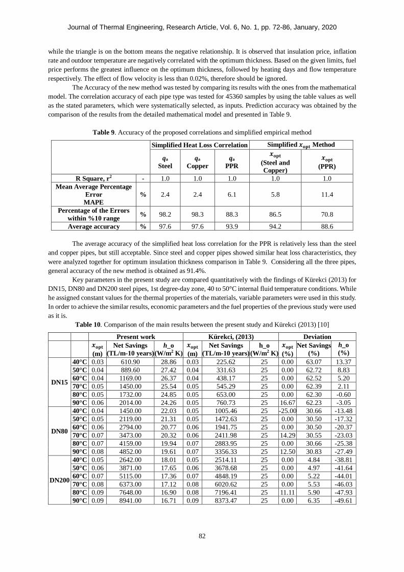
The Accuracy of the new method was tested by comparing its results with the ones from the mathematical model. The correlation accuracy of each pipe type was tested for 45360 samples by using the table values as well as the stated parameters, which were systematically selected, as inputs. Prediction accuracy was obtained by the comparison of the results from the detailed mathematical model and presented in Table 9.

Table 9. Accuracy of the proposed correlations and simplified empirical method

Simplified Heat Loss Correlation Simplified 𝒙𝒙𝐨𝐨𝐨𝐨𝐨𝐨 Method

qa Steel

qa Copper

qa PPR

𝒙𝒙𝐨𝐨𝐨𝐨𝐨𝐨 (Steel and Copper)

𝒙𝒙𝐨𝐨𝐨𝐨𝐨𝐨 (PPR)

R Square, r2 - 1.0 1.0 1.0 1.0 1.0 Mean Average Percentage

Error MAPE

% 2.4 2.4 6.1 5.8 11.4

Percentage of the Errors within %10 range % 98.2 98.3 88.3 86.5 70.8

Average accuracy % 97.6 97.6 93.9 94.2 88.6 The average accuracy of the simplified heat loss correlation for the PPR is relatively less than the steel

and copper pipes, but still acceptable. Since steel and copper pipes showed similar heat loss characteristics, they were analyzed together for optimum insulation thickness comparison in Table 9. Considering all the three pipes, general accuracy of the new method is obtained as 91.4%.

Key parameters in the present study are compared quantitatively with the findings of Kürekci (2013) for DN15, DN80 and DN200 steel pipes, 1st degree-day zone, 40 to 50°C internal fluid temperature conditions. While he assigned constant values for the thermal properties of the materials, variable parameters were used in this study. In order to achieve the similar results, economic parameters and the fuel properties of the previous study were used as it is.

Table 10. Comparison of the main results between the present study and Kürekci (2013) [10]

Present work Kürekci, (2013) Deviation 𝒙𝒙𝐨𝐨𝐨𝐨𝐨𝐨

(m) Net Savings

(TL/m-10 years) h_o

(W/m2 K) 𝒙𝒙𝐨𝐨𝐨𝐨𝐨𝐨 (m)

Net Savings (TL/m-10 years)

h_o (W/m2 K)

𝒙𝒙𝐨𝐨𝐨𝐨𝐨𝐨 (%)

Net Savings (%)

h_o (%)

DN15

40°C 0.03 610.90 28.86 0.03 225.62 25 0.00 63.07 13.37 50°C 0.04 889.60 27.42 0.04 331.63 25 0.00 62.72 8.83 60°C 0.04 1169.00 26.37 0.04 438.17 25 0.00 62.52 5.20 70°C 0.05 1450.00 25.54 0.05 545.29 25 0.00 62.39 2.11 80°C 0.05 1732.00 24.85 0.05 653.00 25 0.00 62.30 -0.60 90°C 0.06 2014.00 24.26 0.05 760.73 25 16.67 62.23 -3.05

DN80

40°C 0.04 1450.00 22.03 0.05 1005.46 25 -25.00 30.66 -13.48 50°C 0.05 2119.00 21.31 0.05 1472.63 25 0.00 30.50 -17.32 60°C 0.06 2794.00 20.77 0.06 1941.75 25 0.00 30.50 -20.37 70°C 0.07 3473.00 20.32 0.06 2411.98 25 14.29 30.55 -23.03 80°C 0.07 4159.00 19.94 0.07 2883.95 25 0.00 30.66 -25.38 90°C 0.08 4852.00 19.61 0.07 3356.33 25 12.50 30.83 -27.49

DN200

40°C 0.05 2642.00 18.01 0.05 2514.11 25 0.00 4.84 -38.81 50°C 0.06 3871.00 17.65 0.06 3678.68 25 0.00 4.97 -41.64 60°C 0.07 5115.00 17.36 0.07 4848.19 25 0.00 5.22 -44.01 70°C 0.08 6373.00 17.12 0.08 6020.62 25 0.00 5.53 -46.03 80°C 0.09 7648.00 16.90 0.08 7196.41 25 11.11 5.90 -47.93 90°C 0.09 8941.00 16.71 0.09 8373.47 25 0.00 6.35 -49.61


83

Table 10 shows the deviations between Kürekci (2013) and the present study. While the deviations for optimum insulation thickness (x_opt ) are in an acceptable range, larger deviations exist for net savings. The reason for the deviations is the difference between the parameters used in two studies. External surface heat transfer coefficient (ho) has an important influence on heat loss and that changes both net savings and x_opt values. Although Kürekci (2013) assigned a constant value to ho for the simplicity, in this study the same parameter was calculated with respect to the pipes exposed to 17.74°C and 5m/s windy environmental conditions. CONCLUSION

Reducing the heat losses to a minimum in hot water piping systems is important in order to reduce the environmental impact and costs, as well as ensuring the energy security. With mathematical modeling techniques, the most suitable solution can be found with high accuracy. In this study, a mathematical model was developed to calculate the optimum insulation thickness for insulated hot water piping systems in ambient air. Then, the results of the mathematical model and the empirical method were compared with regard to the derived combinations. A similar study can be conducted for larger pipes, wet steam and superheated steam flows. The following conclusions were drawn from this study:

• The standard optimum insulation thickness for the tested conditions was determined between 2.5 and 10cm. The unit price per cubic meter was used for calculation of insulation cost. Insulation material prices in the market vary considerably depending on the diameter and thickness of the insulation layer. Including the variable unit price of insulation material in the calculations can improve the accuracy of similar studies.

• Application of insulation with optimum thickness to steel, copper and PPR pipes reduces the heat losses by 89, 88 and 83% respectively. Considering a DN200 steel pipe with an internal flow temperature of 90°C, in a windless -10°C environment, which is operated whole year, the heat losses can be reduced by 86% and 95% after the application of 2.5cm and 10cm glass wool insulation respectively.

• Due to their relatively higher thermal conductivity, steel and copper pipes showed similar heat loss characteristics, therefore the optimum insulation thickness values were calculated close to each other. While the thermal conductivity of the PPR pipe is 98% less than the steel pipe, the average heat loss from uninsulated PPR was calculated only 38% less.

• Fuel type has a direct impact on costs, through the fuel prices and heating system efficiency. Based on the current market conditions in Turkey, using fuel-oil, instead of natural gas, increases the optimum insulation thickness requirement of steel pipes, on average, by 53%.

• The prediction accuracy of the proposed empirical method was verified by the mathematical model. The results from the simple empirical method and the complex mathematical model showed a good agreement. Consequently, the proposed empirical method can be used a universal and practical guide for readers in the determination of thermo-economic thickness of pipe insulation.

NOMENCLATURE A Heat transfer area (m2) C Cost (USD/a) CC Cost Coefficient Ca Annual fuel cost (USD/a) CF Unit cost of fuel (USD/m3), (USD/kg) Cinv Investment cost (USD) Cins Unit cost of insulation (USD/m3) C𝑡𝑡 Total cost (USD) D Hydraulic diameter (m) f Darcy friction factor ΔT Temperature difference (K) 𝑔𝑔 Inflation rate (%) 𝑔𝑔∗ Gravitational acceleration (m/s2) Gr Grasshof number h Convection heat transfer coefficient (W/m2 K) HD Heating days [day] Hu Lower heating value of the fuel (kJ/m3)


84

𝑖𝑖 Interest rate (%) k Thermal conductivity (W/m K) k1 Thermal conductivity of the pipe material (W/m K) k2 Thermal conductivity of the insulation material (W/m K) L Length of pipe (m) 𝑚𝑚𝑎𝑎 Annual fuel consumption (m³/a) N Lifetime (years) Nu Nusselt number Pr Prandtl number PWF Present Worth Factor q Heat loss per unit length (W/m) Q Heat loss (W) 𝑟𝑟 Interest adjusted inflation rate (%) r1 Pipe internal radius (m) r2 Pipe external radius (m) r3 Insulation external radius (m) Ra Rayleigh number R Thermal resistance (m2K/W) Re Reynolds number PP Payback period T Temperature (K) U Total heat transfer coefficient (W/m2K) u Flow velocity (m/s) uwind Wind velocity (m/s) WSF Wind Speed Factor xopt Optimum insulation thickness (m) 𝜀𝜀p Effective roughness of the pipe (m) ε Surface emissivity η Efficiency of the heating system (%) 𝜇𝜇 Fluid dynamic viscosity (kg/ms) 𝜌𝜌 Fluid density (kg/m3) 𝛽𝛽 Thermal expansion coefficient (1/K) 𝜎𝜎 Stefan–Boltzmann constant (𝜎𝜎 = 5.67. 10−8 𝑊𝑊/𝑚𝑚²) a Annual amb Ambient air av Average conv Convection F Fuel inv Investment ins Insulation i Inside o Outside opt Optimum p Pipe rad Radiation s Surface t Total unins Uninsulated REFERENCES [1] World energy statistics, IEA World Energy Statistics and Balances, 2016; doi:10.1787/03a28cba-en. [2] Kaygusuz K., Avci A. C., Potential and utilization of solar energy policies in Turkey, Journal of Engineering Research and Applied Science, 2019; 8(1), 1087-1098. [3] Energy Saver: Tips on Saving Money & Energy at Home (Book), U.S. Department of Energy, 2014; pp. 7–11., doi:10.2172/1134089. [4] Masatin, V., Volkova, A., Hlebnikov, A., Latosov, E., Improvement of district heating network energy efficiency by pipe insulation renovation with PUR foam shells, Energy Procedia, 2017; 113, 265-269. [5] Zhang, L., Wang, Z., Yang, X., Jin, L., Zhang, Q., Hu, W., Thermo-economic analysis for directly-buried pipes insulation of district heating piping systems, Energy Procedia, 2017; 105, 3369-3376.


85

[6] Daşdemir, A., Ural, T., Ertürk, M., Keçebaş, A., Optimal economic thickness of pipe insulation considering different pipe materials for HVAC pipe applications. Applied Thermal Engineering, 2017; 121, 242-254. [7] Öztürk, İ. T., Karabay, H., Bilgen, E., Thermo-economic optimization of hot water piping systems: A comparison study, Energy, 2006; 31(12), 2094-2107. [8] Özel, G., Açıkkalp, E., Görgün, B., Yamık, H., Caner, N., Optimum insulation thickness for piping system using exergy and environmental methods, International Journal of Global Warming, 2017; 11(1), 107-123. [9] Keçebaş, A., Alkan, M. A., Bayhan, M., Thermo-economic analysis of pipe insulation for district heating piping systems, Applied Thermal Engineering, 2011; 31(17-18), 3929-3937. [10] Kürekci N.A., Türkiye’nin Dört Derece Gün Bölgesinde Borular İçin Optimum Yalıtım Kalınlığı, TMMOB Tesisat Mühendisliği Dergisi, 2013; vol. 136, pp. 25-40. [11] Stainless Steel Pipes Measures and Features, Stainless Steel Pipes, www.steellines.com/stainless_steel_pipes-s106.html. [12] Çakmanus, İ., İman H.,Mekanik Tesisat Sistemlerinde Kullanılan Borular, Türk Tesisat Mühendisleri Dernegi, Vol. 33, Issue 10. [13] PPR-C Pipes and Fittings, Plastherm, www.plastherm.com/pprc-pipes-and-fittings/. [14]PPRC Pipe – Pipes - Fırat Plastic, www.firat.com/en-us/indoor-piping-system/cold-hot-water-pipe-systems/pprc-product-range/pprc-pipe?section=374. [15]HDPE-Pipe-for-Water-Supply-Dimension, PPR Pipe Fittings, C&N Aquatherm, www.pprpipefittings.com/wp-content/uploads/2015/07/HDPE-Pipe-for-water-supply-dimension.jpg. [16] Cengel, Y. A., Klein, S., Beckman, W., Heat transfer: a practical approach, 1998; Vol. 141, New York: McGraw-Hill. [17] Churchill, Stuart W., Humbert H.s. Chu., Correlating equations for laminar and turbulent free convection from a horizontal cylinder, International Journal of Heat and Mass Transfer, 1975; Vol. 18, Issue 9, 1975, pp. 1049–1053. [18] Churchill, S. W., M. Bernstein., A Correlating Equation for Forced Convection from Gases and Liquids to a Circular Cylinder in Crossflow, Journal of Heat Transfer,1977; Vol. 99, Issue 2, pp. 300. doi:10.1115/1.3450685. [19] Emissivity Table, ThermoWorks, 2018; www.thermoworks.com/emissivity_table. [20] PPR Piping System, Mechanical Properties and Application Information for Niron PPR, PPR Supply, 2016; pprsupply.com/content/mechanical properties and application information for niron ppr 2016.pdf. [21]Specification - Insulation of Pipe & Duct Work XPE/IXPE, Proflex Thermal Insulation, proflexinsulation.com/specifications/. [22]Polietilen Boru İzoleleri, KAR-EL Klimaflexler Güncel Fiyat Listesi, 2018;www.kar-el.com.tr/fliste2.aspx?id=244. [23] Yakıt Fiyatları Karşılaştırması, Igdas, 2017; www.igdas.istanbul/yakit-fiyatlari-karsilastirmasi/index.html/. [24] Ashouri, M., Astaraei, F. R., Ghasempour, R., Ahmadi, M. H., Feidt, M. Optimum insulation thickness determination of a building wall using exergetic life cycle assessment, Applied Thermal Engineering, 2016; 106, pp. 307-315. [25] OECD Long-Term interest rates, Main Economic Indicators, 2007; Vol. 2017, Issue 7, doi:10.1787/mei-v2017-7-en.


86

APPENDIX Table 11. Wind speed factor

Wind Speed [m/s] 0 1 2 3 4 5 WSF, stainless steel pipe 0.8626 0.9356 0.9555 0.9646 0.9701 0.9739

WSF, copper pipe 0.8661 0.9389 0.9577 0.9664 0.9717 0.9753 WSF, PPR pipe 0.7905 0.8566 0.8727 0.8804 0.8847 0.8877

Table 122. Present worth factor

Inflation Rate, g (%)

Inte

rest

Rat

e, i

(%)

% -1 0 2 4 6 8 10 12 14 16 18 20 -1 1.01 9.47 8.52 7.70 7.00 6.12 5.86 5.40 4.99 4.63 4.31 4.03 0 9.47 1.00 8.98 8.11 7.36 6.42 6.15 5.65 5.22 4.83 4.49 4.19 2 8.52 8.98 0.98 9.00 8.14 7.07 6.76 6.20 5.71 5.27 4.89 4.55 4 7.70 8.11 9.00 0.96 9.02 7.79 7.44 6.80 6.25 5.76 5.33 4.95 6 7.00 7.36 8.14 9.02 0.94 8.61 8.20 7.48 6.85 6.30 5.81 5.38 8 6.39 6.71 7.40 8.17 9.04 9.51 9.05 8.23 7.52 6.89 6.35 5.86 10 5.86 6.15 6.76 7.44 8.20 9.51 0.91 9.07 8.26 7.55 6.94 6.39 12 5.40 5.65 6.20 6.80 7.48 8.64 9.07 0.89 9.08 8.29 7.59 6.98 14 4.99 5.22 5.71 6.25 6.85 7.88 8.26 9.08 0.88 9.10 8.31 7.62 16 4.63 4.83 5.27 5.76 6.30 7.22 7.55 8.29 9.10 0.86 9.11 8.34 18 4.31 4.49 4.89 5.33 5.81 6.63 6.94 7.59 8.31 9.11 0.85 9.13 20 4.03 4.19 4.55 4.95 5.38 6.12 6.39 6.98 7.62 8.34 9.13 0.83

Table 13. Optimum insulation thickness (𝑥𝑥opt) of the pipe [mm], corresponding to the Cost Coefficient

Nominal Pipe Size DN15 DN20 DN25 DN32 DN40 DN50 DN65 DN80 DN100 DN125 DN150 DN200

Cos

t Coe

ffici

ent,

CC

0.05 6 6 6 6 6 6 7 7 7 7 7 7 0.10 8 8 8 8 9 9 9 9 9 9 9 10 0.15 9 9 10 10 10 11 11 11 11 11 12 12 0.50 15 16 16 17 17 18 18 19 19 20 20 21

1 20 21 22 23 23 24 25 25 26 27 28 28 5 37 39 41 43 44 46 48 50 52 54 55 58 10 48 51 53 56 58 61 64 66 69 72 74 77 15 56 59 62 66 68 71 75 77 81 85 88 92 20 63 66 70 73 76 79 84 86 91 95 98 103 25 68 72 76 80 82 87 91 94 100 104 108 113 30 73 77 81 86 88 93 98 101 107 112 116 122 35 78 82 86 91 94 99 104 108 114 119 123 130 40 82 86 91 96 99 104 110 113 120 125 130 137 45 86 90 95 100 103 109 115 119 126 131 136 144 50 89 94 99 105 108 113 119 124 131 137 142 150 55 93 98 103 108 112 118 124 128 136 142 148 156 60 96 101 106 112 115 122 128 133 140 147 153 161 65 99 104 110 116 119 125 132 137 145 151 158 166 70 102 107 113 119 123 129 136 141 149 156 162 171 75 104 110 116 122 126 132 140 145 153 160 166 176 80 107 113 119 125 129 136 143 148 157 164 171 181 85 110 115 121 128 132 139 146 152 161 168 175 185 90 112 118 124 131 135 142 150 155 164 172 179 189 95 114 121 127 134 138 145 153 158 168 175 183 193 100 117 123 129 136 140 148 156 161 171 179 186 197 105 119 125 132 139 143 151 159 165 174 182 190 201 110 121 128 134 142 146 153 162 168 178 186 194 205 115 123 130 136 144 148 156 164 170 180 189 197 208 120 124 130 137 145 149 157 165 171 181 190 198 209

a practical method for determination of economic

Documents