A Practical Implementation of ParallelOrdered Maps and Sets with just Join

Bachelor Thesis of

Daniel Ferizovic

At the Department of InformaticsInstitute for Theoretical Computer Science

Reviewer: Prof. Dr.rer.nat. Peter SandersSecond reviewer: Prof. Dr. Dorothea WagnerAdvisor: Prof. Dr.rer.nat. Peter SandersSecond advisor: Prof. Guy Blelloch

Duration: December 15th, 2015 – March 10th, 2016

KIT – University of the State of Baden-Wuerttemberg and National Research Center of the Helmholtz Association www.kit.edu

I declare that I have developed and written the enclosed thesis completely by myself, andhave not used sources or means without declaration in the text.

Karlsruhe, March 14, 2016

. . . . . . . . . . . . . . . . . . . . . . . . . . . . . . . . . . . . . . . . .(Daniel Ferizovic)

Contents

1. Introduction 3

2. Acknowledgements 5

3. Preliminaries 73.1. Binary Search Tree . . . . . . . . . . . . . . . . . . . . . . . . . . . . . . . . 7

3.2. Balanced Binary Search Trees . . . . . . . . . . . . . . . . . . . . . . . . . . 8

3.2.1. AVL Tree . . . . . . . . . . . . . . . . . . . . . . . . . . . . . . . . . 8

3.2.2. Weight-Balanced Tree . . . . . . . . . . . . . . . . . . . . . . . . . . 8

3.2.3. Red-Black Tree . . . . . . . . . . . . . . . . . . . . . . . . . . . . . . 8

3.2.4. Treap . . . . . . . . . . . . . . . . . . . . . . . . . . . . . . . . . . . 9

3.3. Basic Operations on BSTs . . . . . . . . . . . . . . . . . . . . . . . . . . . . 9

3.3.1. Tree rotations . . . . . . . . . . . . . . . . . . . . . . . . . . . . . . . 9

3.4. Ordered Set . . . . . . . . . . . . . . . . . . . . . . . . . . . . . . . . . . . . 10

3.5. Ordered Map . . . . . . . . . . . . . . . . . . . . . . . . . . . . . . . . . . . 10

3.6. Lockfree Data Structures . . . . . . . . . . . . . . . . . . . . . . . . . . . . 10

3.7. Persistence . . . . . . . . . . . . . . . . . . . . . . . . . . . . . . . . . . . . 11

3.8. Garbage Collection . . . . . . . . . . . . . . . . . . . . . . . . . . . . . . . . 11

3.9. Parallel Computation Model . . . . . . . . . . . . . . . . . . . . . . . . . . . 11

4. Related Work 13

5. The Join Operation 155.1. AVL Trees . . . . . . . . . . . . . . . . . . . . . . . . . . . . . . . . . . . . . 16

5.2. Red-Black Tree . . . . . . . . . . . . . . . . . . . . . . . . . . . . . . . . . . 16

5.3. Weight-Balanced Tree . . . . . . . . . . . . . . . . . . . . . . . . . . . . . . 17

5.4. Treap . . . . . . . . . . . . . . . . . . . . . . . . . . . . . . . . . . . . . . . 18

5.5. Operations using Join . . . . . . . . . . . . . . . . . . . . . . . . . . . . . . 19

5.5.1. Split . . . . . . . . . . . . . . . . . . . . . . . . . . . . . . . . . . . . 19

5.5.2. Union . . . . . . . . . . . . . . . . . . . . . . . . . . . . . . . . . . . 20

5.5.3. Intersect . . . . . . . . . . . . . . . . . . . . . . . . . . . . . . . . . . 20

5.5.4. Difference . . . . . . . . . . . . . . . . . . . . . . . . . . . . . . . . . 21

5.5.5. Insert . . . . . . . . . . . . . . . . . . . . . . . . . . . . . . . . . . . 22

5.5.6. Delete . . . . . . . . . . . . . . . . . . . . . . . . . . . . . . . . . . . 22

5.5.7. Range . . . . . . . . . . . . . . . . . . . . . . . . . . . . . . . . . . . 22

5.5.8. Filter . . . . . . . . . . . . . . . . . . . . . . . . . . . . . . . . . . . 22

5.5.9. Build . . . . . . . . . . . . . . . . . . . . . . . . . . . . . . . . . . . 23

6. Implementation Details 256.1. Our library . . . . . . . . . . . . . . . . . . . . . . . . . . . . . . . . . . . . 25

6.2. Persistence . . . . . . . . . . . . . . . . . . . . . . . . . . . . . . . . . . . . 26

v

vi Contents

6.3. Memory management . . . . . . . . . . . . . . . . . . . . . . . . . . . . . . 276.3.1. Reference count collection . . . . . . . . . . . . . . . . . . . . . . . . 27

7. Library Interface 297.1. Method Summary . . . . . . . . . . . . . . . . . . . . . . . . . . . . . . . . 30

8. Evaluation 338.1. Setting . . . . . . . . . . . . . . . . . . . . . . . . . . . . . . . . . . . . . . . 338.2. Comparing different trees . . . . . . . . . . . . . . . . . . . . . . . . . . . . 338.3. Comparing functions . . . . . . . . . . . . . . . . . . . . . . . . . . . . . . . 348.4. Comparing to STL . . . . . . . . . . . . . . . . . . . . . . . . . . . . . . . . 368.5. Comparing to parallel implementations . . . . . . . . . . . . . . . . . . . . . 38

9. Conclusion 41

Bibliography 43

Appendix 45A. Examples . . . . . . . . . . . . . . . . . . . . . . . . . . . . . . . . . . . . . 45

vi

Contents 1

1

1. Introduction

Modern programming languages nowdays offer support for a variety of data types. Maps,also refered as dictionaries or associative arrays are one of them. Some languages havethem built in as part of the language, while other offer support through libraries. Alongwith maps, libraries often provide implementations of the set data type. Since sets canbe viewed as a special kind of an associative container (with unit value associated witheach key), they are often implemented as maps. For this reason, from now on we willdirect our focus on maps, but note that most things we say also apply for sets. The mapdata type usually comes in two distinct flavours, it can be either ordered or unordered.An ordered map has a total ordering imposed on the key set of its entries. This can bevery useful in practice, since it allows various types of queries based on the key ordering.For example functions like range, rank, select, next/previous-key are usually supported byordered maps. They are often implemented using some kind of balanced binary search treeas their underlying data structure. This makes most of the operations offered by orderedmaps take O(log n) time. Unordered maps on the other hand have no ordering imposedon their key set. They are usually implemented using hash tables, such that operationslike insert and remove take expected O(1) time. The faster time for insertion and removalis favourable for unordered maps, but it often pays off only for a large number of suchoperations.

In this paper we describe and implement a parallel library for ordered maps and sets.We compare four different balanced binary search trees (BBST) to see which achievesthe best performance. This includes AVL trees, weight-balanced trees, red-black trees andtreaps. All core library functions are implemented around a single function called join3. Ittakes two balanced binary search trees T1 and T2, and an additional key k as arguments,and returns a balanced binary search tree T such that K(T ) = K(T1) ∪ k ∪ K(T2),where K() stands for the key set of a tree. For each BBST we only have to provide animplementation of join3 in order to gain support for all other library functions. Themain reason to implement the interface around join3 wasn’t solely the minimal effortfor supporting multiple BBSTs. Aggregate set functions, such as union, intersect anddifference can be highly paralellized for ordered trees if implemented using join3. Thealgorithms we use for union, intersect and difference achieve a work of O(n log(mn + 1))and a depth of O(logm log n), where m is the size of the larger tree. We note that thiswork is optimal in the comparsion model. These set operations are usually implementedby finger tracing through two sorted sequences simultaneously. This approach is fast inpractice and takes O(n + m) time. However, this complexity is worse than ours when it

3

4 1. Introduction

comes to merging smaller with larger trees. Our experiments (see Chapter 8) also confirmthat. Another issue with this approach is that it returns a sorted sequence and not a tree.We note that those issues only occur in the naive sequential implementation. A lot of workhas been done in parallelizing bulk operations for certain search trees. Bulk insertions,for example, can be viewed as the union of one tree with another, since it achieves thesame effect. To see which of these approaches is more efficient we also compare ourselfto state of the art parallel search trees (see Chapter 4). Among other functions that weparallelized are build, filter and forall. In order for our library to be useful in practicewe made all operations persistent. That is, taking the union of two maps does not sideeffect the input maps. Persistence can be useful in many applications. For example, if wehave two tables in our database, we probably don’t want them to be completly destroyedafter taking a single intersection or union of them.

In Chapter 4 we talk more about related research and the work which has been done inthis area. Chapter 5 describes the join3 operation and how it can be realized for thedifferent types of balanced search trees. We also talk about how other operations can beimplemented by using only join3. Chapter 6 describes the implementation details of ourlibrary. We talk about the memory management and how exactly we achieved persistancefor the data structures. An overview of our library interface can be found in Chapter 7.and at last, in Chapter 8 we show the experimental results we have performed with ourlibrary.

4

2. Acknowledgements

I would like to thank Prof. Guy Blelloch from the Carnegie Mellon University for givingme useful advice and guidance during my work on this thesis. Thanks also goes to YihanSun for providing proofs for the running times of several algorithms.

5

3. Preliminaries

3.1. Binary Search Tree

A binary search tree (BST) is a rooted tree in which every node has at most two children,refered as left and right child. A node without a left and right child is called leaf node.We refer with the left (right) subtree of a node to the rooted tree starting at its left (right)child. Each node of a binary search tree has an unique key k ∈ Ω associated with it. Werequire Ω to be a totally ordered set. Additionaly, each node is able to store some extrainformation, refered as value.

From now, if not otherwise stated, we will use the large capital letter T to denote a BSTand lowercase letters u, v ∈ T , to refer to nodes. Let v ∈ T be a node of T. We introducethe following notation:

• v.left represents the left child (or subtree) of v.

• v.right represents the right child (or subtree) of v.

• v.key represents the key associated with v.

In general, if we intruduce a property prop to nodes we will refer to it as v.prop.

Every binary search tree has to satisfy the so called BST-property. It states that for everynode v ∈ T the following holds:

∀u ∈ v.left : v.key ≥ u.key ∧ ∀u ∈ v.right : v.key ≤ u.key

The height of a binary search tree is defined as the length of the longest path from theroot to any other node in T. Similary, the height of a node v ∈ T is defined to be equalto the height of the tree rooted at v. For convinience we introduce the following notationfor a BST:

• T.root represents the root of T.

• T.height represents the height of T.

• T.prop will be used as a short form for T.root.prop.

• K(T) is the set of all keys present in T .

• V(T) is the set of all values present in T .

7

8 3. Preliminaries

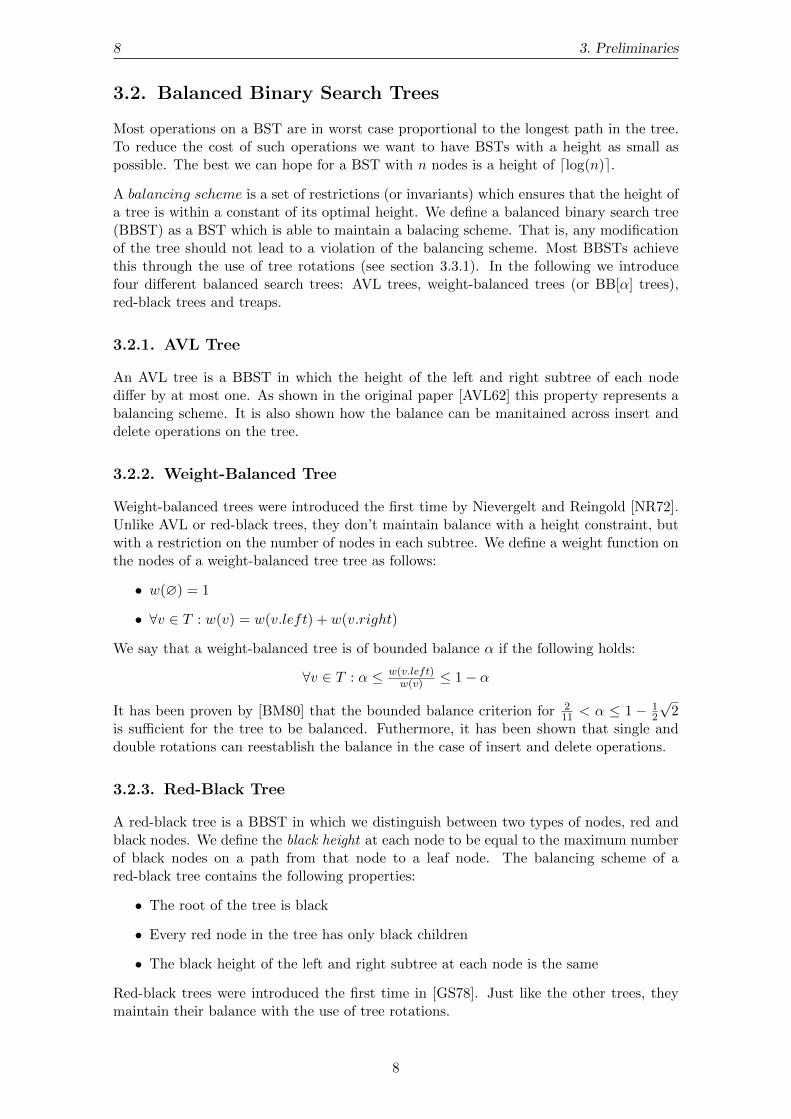
3.2. Balanced Binary Search Trees

Most operations on a BST are in worst case proportional to the longest path in the tree.To reduce the cost of such operations we want to have BSTs with a height as small aspossible. The best we can hope for a BST with n nodes is a height of dlog(n)e.

A balancing scheme is a set of restrictions (or invariants) which ensures that the height ofa tree is within a constant of its optimal height. We define a balanced binary search tree(BBST) as a BST which is able to maintain a balacing scheme. That is, any modificationof the tree should not lead to a violation of the balancing scheme. Most BBSTs achievethis through the use of tree rotations (see section 3.3.1). In the following we introducefour different balanced search trees: AVL trees, weight-balanced trees (or BB[α] trees),red-black trees and treaps.

3.2.1. AVL Tree

An AVL tree is a BBST in which the height of the left and right subtree of each nodediffer by at most one. As shown in the original paper [AVL62] this property represents abalancing scheme. It is also shown how the balance can be manitained across insert anddelete operations on the tree.

3.2.2. Weight-Balanced Tree

Weight-balanced trees were introduced the first time by Nievergelt and Reingold [NR72].Unlike AVL or red-black trees, they don’t maintain balance with a height constraint, butwith a restriction on the number of nodes in each subtree. We define a weight function onthe nodes of a weight-balanced tree tree as follows:

• w(∅) = 1

• ∀v ∈ T : w(v) = w(v.left) + w(v.right)

We say that a weight-balanced tree is of bounded balance α if the following holds:

∀v ∈ T : α ≤ w(v.left)w(v) ≤ 1− α

It has been proven by [BM80] that the bounded balance criterion for 211 < α ≤ 1 − 1

2

√2

is sufficient for the tree to be balanced. Futhermore, it has been shown that single anddouble rotations can reestablish the balance in the case of insert and delete operations.

3.2.3. Red-Black Tree

A red-black tree is a BBST in which we distinguish between two types of nodes, red andblack nodes. We define the black height at each node to be equal to the maximum numberof black nodes on a path from that node to a leaf node. The balancing scheme of ared-black tree contains the following properties:

• The root of the tree is black

• Every red node in the tree has only black children

• The black height of the left and right subtree at each node is the same

Red-black trees were introduced the first time in [GS78]. Just like the other trees, theymaintain their balance with the use of tree rotations.

8

3.3. Basic Operations on BSTs 9

3.2.4. Treap

Treaps are randomized binary search trees [SA96]. Each node has an number assigned toit, which we call priority. The nodes of a treap must statisfy the heap property:

∀v ∈ T : v.priority ≥ v.left.priority ∧ v.priority ≥ v.right.priority

If the priorities are assigned uniformly at random, it can be shown that such a tree hasan expected height of O(log n).

3.3. Basic Operations on BSTs

There are three basic operations that a BST is required to support: find, insert anddelete. They are are implemented using a tree traversal on the key order. We describethe algorithm for find below:

1 Procedure find (key)2 return search(root, key)3

4 Procedure search(curr, key)5 if curr ==⊥: then False;6 else if curr.key < key: then search(curr.right, key)7 else if curr.key > key: then search(curr.left, key)8 else True ;

Algorithm 3.1: Finding a key in a BST

Insert is implemented by finding the proper position in the tree where the key needs to beplaced, similar to the find algorithm. If the key is already present we do nothing, otherwisewe create a new node.

Delete is a bit more complicated, since we can’t just remove a node from the middle of atree. The problem is that we don’t have a place to reattach the subtrees from the deletednode. We observe the following cases:

• The node has no childrern. The node can be immediately removed.

• The node has one child. We delete the node and assign the child to the parent ofthe removed node.

• The node has two childrern. We find the in-order successor of the node which shouldbe removed and swap the keys of the two nodes. We then procceed by deleting thesuccessor node at the lower level until we reach one of the first two base cases.

We note that insert and delete as described above are quite general. Applying them toany of the mentioned BBSTs will most likely lead to a violation of the defining properties.For example, the height of the subtree in which the node is inserted might increase by one.This could violate the balancing scheme of AVL trees. Similary, the key inserted into atreap following only the key order might violate the heap property. This is usually solvedby applying one or more tree rotations.

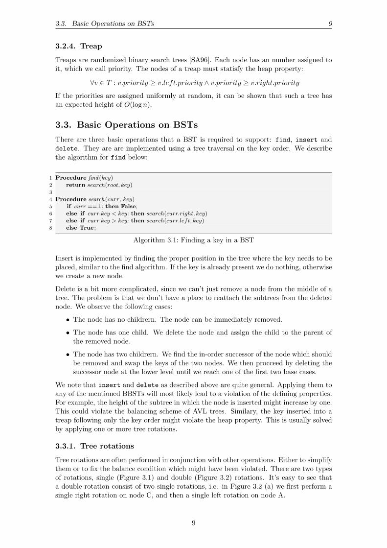
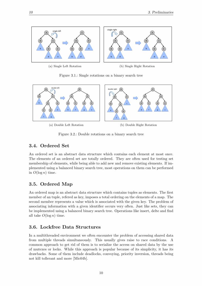
3.3.1. Tree rotations

Tree rotations are often performed in conjunction with other operations. Either to simplifythem or to fix the balance condition which might have been violated. There are two typesof rotations, single (Figure 3.1) and double (Figure 3.2) rotations. It’s easy to see thata double rotation consist of two single rotations, i.e. in Figure 3.2 (a) we first perform asingle right rotation on node C, and then a single left rotation on node A.

9

10 3. Preliminaries

C

A E

B D

b d

e

A

B C

D E

d e

b

single left

(a) Single Left Rotation

C

A E

B D

single right

b d

e

A

B C

D E

d e

b

(b) Single Right Rotation

Figure 3.1.: Single rotations on a binary search tree

A

B C

D E

e

b

double left

F G

f g

D

A C

G E

e b

F

f g

B

(a) Double Left Rotation

A

B

E D

d F G

f g

E

B A

G C

c d

F

f g

D

C

c

double right

(b) Double Right Rotation

Figure 3.2.: Double rotations on a binary search tree

3.4. Ordered Set

An ordered set is an abstract data structure which contains each element at most once.The elements of an ordered set are totally ordered. They are often used for testing setmembership of elements, while being able to add new and remove existing elements. If im-plemented using a balanced binary search tree, most operations on them can be performedin O(log n) time.

3.5. Ordered Map

An ordered map is an abstract data structure which contains tuples as elements. The firstmember of an tuple, refered as key, imposes a total ordering on the elements of a map. Thesecond member represents a value which is associated with the given key. The problem ofassociating information with a given identifier occurs very often. Just like sets, they canbe implemented using a balanced binary search tree. Operations like insert, delte and findall take O(log n) time.

3.6. Lockfree Data Structures

In a multithreaded environment we often encounter the problem of accessing shared datafrom multiple threads simultaneously. This usually gives raise to race conditions. Acommon approach to get rid of them is to serialize the access on shared data by the useof mutexes or locks. While this approach is popular because of its simplicity, it has itsdrawbacks. Some of them include deadlocks, convoying, priority inversion, threads beingnot kill tollerant and more [Mic04b].

10

3.7. Persistence 11

Lockfree data structures don’t suffer from any of the mentioned drawbacks. They providethread-safe access without making use of synchronization primitives like mutexes. A lock-free data structure guarantees that at any time at least one thread accessing it is makingprogress. Lock-based data structures fail to satisfy this requirement. Making a data struc-ture lockfree is however more difficult. The reason for this is that we are restricted to asmall set of atomic hardware instructions in order to make the structure thread safe. Oneof the weidely used atomic instruction for this purpose is the compare-and-swap (CAS)primitive. It compares the contents of a memory location to a given value and, only ifthey are the same, modifies the contents of that memory location. Most hardware nowa-days supports a double word compare-and-swap. Lockfree algorithms based on the CASprimitive have been developed for many common data structures, including linked lists,queues, deques and stacks.

3.7. Persistence

When we modify a data structure we usually get a new modified version of it, withoutbeing able to reflect on its previous state. Such data structures are called ephemeral. Allmodifications on an ephemeral data structure apply to the latest and only version of it.Persistence allows us to keep track of old versions of a data structure. It allows us tolookup older versions, and in some cases to even modify them. Depending on what kind ofupdates are supported by the different versions of a data structure, we distinguish betweenthree types of persistence:

Partial persistence allows updates only on the latest version of the data structure (Linearversioning).

Full persistence allows updates on any version of the data structure (Tree versioning).

Confluent persistence allows updates on any version. Additionally it allows melding dif-ferent versions together. (DAG versioning)

3.8. Garbage Collection

A garbage collector (GC) is usually implemented as part of automatic memory manage-ment. It is responsible for reclaiming the memory of objects which are not used by aprogram anymore. We distinguish between two different types of garbage collectors:

• Reference count GC – keeps a reference count to each object in the program. Whenthe reference count to an object becomes zero, the GC immediately reclaims theobject’s memory.

• Tracing GC – maintains a set of root objects, which includes all objects referencedby the call stack and global variables. The GC reclaims memory by periodicallytracing all objects which are reachable from the root set. Everything that was notreached from the root set is considered garbage.

3.9. Parallel Computation Model

The computation model we use is the parallel random access machine (PRAM). It consistof a collection of processors operating on a shared memory. All comunication between theprocessors is done via the shared memory. Our PRAM model is concurrent-read/exclusive-write (CREW) PRAM, which means that multiple threads are allowed to read simultane-ously from the same memory location, but only one thread is allowed to write a memory

11

12 3. Preliminaries

location at the same time. This can be achieved using various synchronisation mecha-nisms. We avoid the use of locks as much as possible and rely on atomic instructions likecompare-and-swap and test-and-set.

We use the work/depth model to express the running times of our algorithms. Work isthe total number of operations performed by an algorithm, while depth represents thelongest strongly sequential chain of operations that an algorithm needs to perform. In thissense, work is equivalent to the sequential time of an algorithm, and depth is equal to therunning time of an algorithm on a machine with an unlimited number of processors.

12

4. Related Work

Implementing a join operation for balanced binary search trees has been studied before.Blelloch and Miller [BRM98] describe how join can be implemented for treaps. Theyintroduce parallel algorithms for union, intersect and difference based on the join operation.All of them take O(n log(mn +1) time, which is optimal in the comparsion model. Similary,in his work [Tar82], Tarjan gives an efficient join-algorithm for red black trees.

A lot of reasearch has been done in the field of concurrent and parallel operations onbinary search trees. Kung and Lehman gave in their work [KL80] a generic approach onhow to implement concurrent safe binary search trees. They study in great detail howto build a concurrent safe system which would support the basic BST operations. Inorder to achieve this, they make use of locks, node copying and back pointers. Some ofthe later research on concurrent search trees includes the work of [BCCO10] and [BE13].Bronson et al. describe a concurrent safe AVL tree which uses hand-over-hand optimisticvalidation along with a relaxed balancing criteria, which reduces the contention on the treeby postponing rebalancing operations. Among other balanced binary search trees whichhave been studied for concurency are red-black trees. Some of the later research in thisarea has been done by Besa [BE13]. He describes a fast implementation of a concurrentred-black tree, which outperforms the previously introduced AVL tree by Bronson.

Besides providing concurrent access, attention has also been given to the parallelization ofcertain operations. Park and Park [PP01] give a highly theoretical description of parallelred-black trees for the PRAM model, including bulk insertion/removal and tree contruc-tion. However, they do not consider implementation related issues, nor they provide anactual implementation of the trees. Later on, Frias and Singler [FS07] have described andimplemented a parallel version of red-black trees. They included their implementation aspart of the MCSTL (Multi Core Standard Template Library), which is to our knowledgeone of the only libraries providing parallel sets and maps for C++. They parallelize bulkupdates by initialy splitting the tree by the update sequence, and then in parallel insert theremaining sequences into the right subtrees. Another interesting library available for C++is the HPC++ which includes the PSTL (Parallel Standard Template Library) [JGB97].The PSTL supports maps and sets, however, it is designed for the distributed setting asopposed to shared memory.

Parallelizing certain operations has not only been limited to binary search trees. Erb etal. introduce in their work [EKS14] a parallelized weight-balanced B-tree. They makeuse of the property that partial reconstruction of weight-balanced B-trees can be done

13

14 4. Related Work

in constant amortized time. This way they avoid the overhead of frequent rebalancingoperations during bulk insertions. Similar work has been done by Akhremtsev et al.[AS15], who studied parallel bulk operations on (a, b)-trees. They parallelize bulk updatesby splitting the input tree into p distinct trees, where p denotes the number of processors.Then they insert the corresponding sequence parts into the individual trees, after whichall of the trees are joined back together. Based on our experimental results, and those ofAkhremtsev, the (a, b)-tree implementaion is the fastest among the parallel search treeswe tested.

When it comes to persistence, groundbreaking work has been done by Driscoll, Sarnak,Sleator and Tarjan [DSST89]. They describe general transformations on how to make anypointer based structure fully persistent. They achieve persistence using O(1) additionalspace per operation with only a constant slowdown. This is however only true for fulland partial persistence. Confluent persistence turned out to be more difficult. Based onthe prior work of DSST, Fiat and Kaplan [FK01] describe the first general transformationfor making any pointer based strcuture confluently persistent. The bounds they achieveare not as good as those of DSST. It is still open if better methods exist in achievingconfluent persistence for specific data strucutres, i.e. BSTs. Due to the lack of efficient(and practical) transformations for confluent persistence, a common and simple way toachieve it is by path copying [ST86]. There are several benefits in this approach: the datastructures are by default safe for concurrency, there is only a constant overhead per accessand it is simple to realize in practice. However, it is not the most space efficient solution.Our maps and sets make use of this approach, as we describe in more detail in Chapter 6.

14

5. The Join Operation

As stated earlier, common operations such as insert, delete and lookup are usually im-plemented using a tree traversal on the key order. In this chapter we introduce the joinoperation and argue that it is sufficient to implement all other set operations. This makesit possible to provide a variety of generic operations on many different balanced searchtrees by implementing just join for each tree. One big advantage of using join is that oper-ations such as union, intersect and difference can be efficiently parallelized if implementedwith join.

We desribe two variations of the join primitive, join2 and join3.

• join3(TL, k, TR) takes two BBSTs and one key as an argument, such that K(TL) <k < K(TR). It returns a BBST T , such that K(T ) = K(TL) ∪ k ∪K(TR). If wewouldn’t care about working with balanced trees, join3 could simply create a newnode with key k and attach TL and TR to the left and right of it. This obivously,will not work in the case of BBSTs. We will show how join3 can be implementedfor AVL trees, red-black trees, treaps and weight-balanced trees.

• join2(TL, TR) is similar to join3 except that it does not take a middle key asan argument. It accepts two BBSTs and returns a BBST T such that K(T ) =K(TL) ∪K(TR). join2 can be implemented using join3 as described below.

1 Procedure join2 (TL, TR)2 if TL ==⊥ return TR;3 if TR ==⊥ return TL;4

5 return join3(join2(TR.left, TL), TR.key, TR.right)

Algorithm 5.1: join2

Theorem 5.0.1 The work of join2 is O(TL.height+TR.height) for all of the below men-tioned implementations of join3.

Proof See [SFB16].

15

16 5. The Join Operation

5.1. AVL Trees

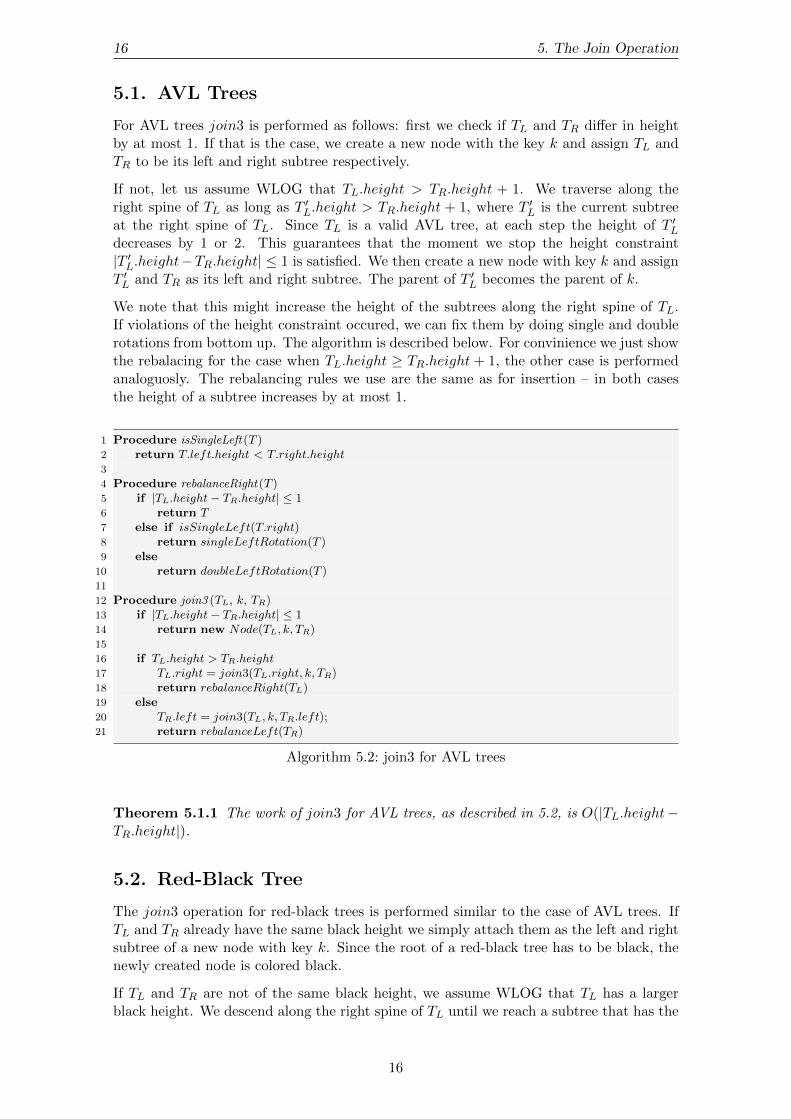
For AVL trees join3 is performed as follows: first we check if TL and TR differ in heightby at most 1. If that is the case, we create a new node with the key k and assign TL andTR to be its left and right subtree respectively.

If not, let us assume WLOG that TL.height > TR.height + 1. We traverse along theright spine of TL as long as T ′

L.height > TR.height + 1, where T ′L is the current subtree

at the right spine of TL. Since TL is a valid AVL tree, at each step the height of T ′L

decreases by 1 or 2. This guarantees that the moment we stop the height constraint|T ′L.height−TR.height| ≤ 1 is satisfied. We then create a new node with key k and assign

T ′L and TR as its left and right subtree. The parent of T ′

L becomes the parent of k.

We note that this might increase the height of the subtrees along the right spine of TL.If violations of the height constraint occured, we can fix them by doing single and doublerotations from bottom up. The algorithm is described below. For convinience we just showthe rebalacing for the case when TL.height ≥ TR.height + 1, the other case is performedanaloguosly. The rebalancing rules we use are the same as for insertion – in both casesthe height of a subtree increases by at most 1.

1 Procedure isSingleLeft (T )2 return T.left.height < T.right.height3

4 Procedure rebalanceRight (T )5 if |TL.height− TR.height| ≤ 16 return T7 else if isSingleLeft(T.right)8 return singleLeftRotation(T )9 else

10 return doubleLeftRotation(T )11

12 Procedure join3 (TL, k, TR)13 if |TL.height− TR.height| ≤ 114 return new Node(TL, k, TR)15

16 if TL.height > TR.height17 TL.right = join3(TL.right, k, TR)18 return rebalanceRight(TL)19 else20 TR.left = join3(TL, k, TR.left);21 return rebalanceLeft(TR)

Algorithm 5.2: join3 for AVL trees

Theorem 5.1.1 The work of join3 for AVL trees, as described in 5.2, is O(|TL.height−TR.height|).

5.2. Red-Black Tree

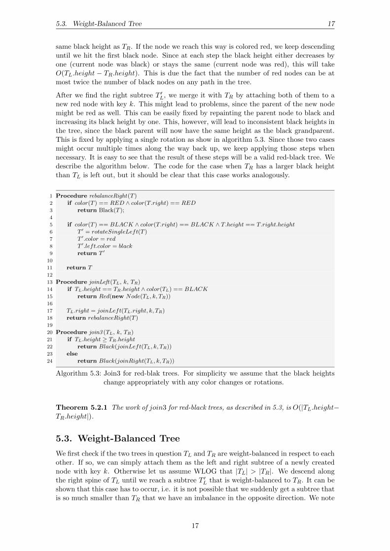
The join3 operation for red-black trees is performed similar to the case of AVL trees. IfTL and TR already have the same black height we simply attach them as the left and rightsubtree of a new node with key k. Since the root of a red-black tree has to be black, thenewly created node is colored black.

If TL and TR are not of the same black height, we assume WLOG that TL has a largerblack height. We descend along the right spine of TL until we reach a subtree that has the

16

5.3. Weight-Balanced Tree 17

same black height as TR. If the node we reach this way is colored red, we keep descendinguntil we hit the first black node. Since at each step the black height either decreases byone (current node was black) or stays the same (current node was red), this will takeO(TL.height − TR.height). This is due the fact that the number of red nodes can be atmost twice the number of black nodes on any path in the tree.

After we find the right subtree T ′L, we merge it with TR by attaching both of them to a

new red node with key k. This might lead to problems, since the parent of the new nodemight be red as well. This can be easily fixed by repainting the parent node to black andincreasing its black height by one. This, however, will lead to inconsistent black heights inthe tree, since the black parent will now have the same height as the black grandparent.This is fixed by applying a single rotation as show in algorithm 5.3. Since those two casesmight occur multiple times along the way back up, we keep applying those steps whennecessary. It is easy to see that the result of these steps will be a valid red-black tree. Wedescribe the algorithm below. The code for the case when TR has a larger black heightthan TL is left out, but it should be clear that this case works analogously.

1 Procedure rebalanceRight (T )2 if color(T ) == RED ∧ color(T.right) == RED3 return Black(T );4

5 if color(T ) == BLACK ∧ color(T.right) == BLACK ∧ T.height == T.right.height6 T ′ = rotateSingleLeft(T )7 T ′.color = red8 T ′.left.color = black9 return T ′

10

11 return T12

13 Procedure joinLeft (TL, k, TR)14 if TL.height == TR.height ∧ color(TL) == BLACK15 return Red(new Node(TL, k, TR))16

17 TL.right = joinLeft(TL.right, k, TR)18 return rebalanceRight(T )19

20 Procedure join3 (TL, k, TR)21 if TL.height ≥ TR.height22 return Black(joinLeft(TL, k, TR))23 else24 return Black(joinRight(TL, k, TR))

Algorithm 5.3: Join3 for red-blak trees. For simplicity we assume that the black heightschange appropriately with any color changes or rotations.

Theorem 5.2.1 The work of join3 for red-black trees, as described in 5.3, is O(|TL.height−TR.height|).

5.3. Weight-Balanced Tree

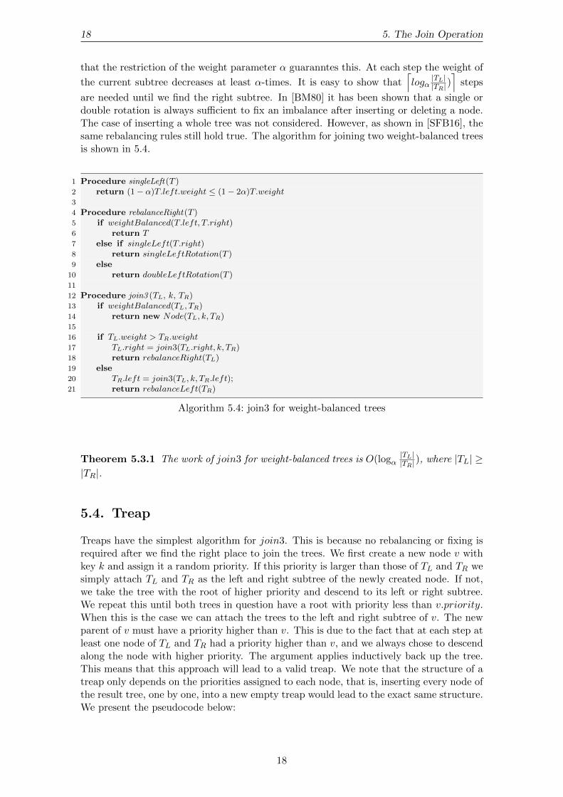
We first check if the two trees in question TL and TR are weight-balanced in respect to eachother. If so, we can simply attach them as the left and right subtree of a newly creatednode with key k. Otherwise let us assume WLOG that |TL| > |TR|. We descend alongthe right spine of TL until we reach a subtree T ′

L that is weight-balanced to TR. It can beshown that this case has to occur, i.e. it is not possible that we suddenly get a subtree thatis so much smaller than TR that we have an imbalance in the opposite direction. We note

17

18 5. The Join Operation

that the restriction of the weight parameter α guaranntes this. At each step the weight of

the current subtree decreases at least α-times. It is easy to show that⌈logα

|TL||TR|)

⌉steps

are needed until we find the right subtree. In [BM80] it has been shown that a single ordouble rotation is always sufficient to fix an imbalance after inserting or deleting a node.The case of inserting a whole tree was not considered. However, as shown in [SFB16], thesame rebalancing rules still hold true. The algorithm for joining two weight-balanced treesis shown in 5.4.

1 Procedure singleLeft (T )2 return (1− α)T.left.weight ≤ (1− 2α)T.weight3

4 Procedure rebalanceRight (T )5 if weightBalanced(T.left, T.right)6 return T7 else if singleLeft(T.right)8 return singleLeftRotation(T )9 else

10 return doubleLeftRotation(T )11

12 Procedure join3 (TL, k, TR)13 if weightBalanced(TL, TR)14 return new Node(TL, k, TR)15

16 if TL.weight > TR.weight17 TL.right = join3(TL.right, k, TR)18 return rebalanceRight(TL)19 else20 TR.left = join3(TL, k, TR.left);21 return rebalanceLeft(TR)

Algorithm 5.4: join3 for weight-balanced trees

Theorem 5.3.1 The work of join3 for weight-balanced trees is O(logα|TL||TR|), where |TL| ≥

|TR|.

5.4. Treap

Treaps have the simplest algorithm for join3. This is because no rebalancing or fixing isrequired after we find the right place to join the trees. We first create a new node v withkey k and assign it a random priority. If this priority is larger than those of TL and TR wesimply attach TL and TR as the left and right subtree of the newly created node. If not,we take the tree with the root of higher priority and descend to its left or right subtree.We repeat this until both trees in question have a root with priority less than v.priority.When this is the case we can attach the trees to the left and right subtree of v. The newparent of v must have a priority higher than v. This is due to the fact that at each step atleast one node of TL and TR had a priority higher than v, and we always chose to descendalong the node with higher priority. The argument applies inductively back up the tree.This means that this approach will lead to a valid treap. We note that the structure of atreap only depends on the priorities assigned to each node, that is, inserting every node ofthe result tree, one by one, into a new empty treap would lead to the exact same structure.We present the pseudocode below:

18

5.5. Operations using Join 19

1 Procedure nodeJoin(TL, u, TR)2 if v.priority > TL.priority ∧ v.priority > TR.priority3 v.left = TL

4 v.right = TR

5 return v6 else if TL.priority > TR.priority7 TL.right = nodeJoin(TL.right, v, TR)8 return TL

9 else10 TR.left = nodeJoin(TL, v, TR.left)11 return TR

12

13 Procedure join3 (TL, k, TR)14 v = new Node(k)15 u.priority = random()16 return nodeJoin(TL, u, TR)

Algorithm 5.5: join3 for treaps

Theorem 5.4.1 The work of join3 for treaps, as described in 5.5, is O(TL.height +TR.height).

5.5. Operations using Join

In this section we will show how to implement other set operations using only the join3primitive. This means that all operations we are going to describe can be generically usedfor all BBSTs we have mentioned. Split is probably the most important operation of them,since it is used as a subroutine in many other set operations.

5.5.1. Split

Split is a function which takes a BST T and a key k as arguments and returns twoBSTs, one containing all nodes with keys less than k, and one containing all nodes withkeys greater than k. Fromally speaking, split(T, k) is a function which returns a triple(TL, f lag, TR), such that K(TL) < k < K(TR). The trees TL and TR contain all nodesfrom T except the node with key k, if it was present at all. The return value of flagis a boolean value indicating whether a node with key k was present in the tree or not.split works recursively by making usage of join3. We do a search for the key on the tree.Lets assume the key is in the left subtree of T , and (TL, f lag, TR) is the result of splittingthe left subtree of T . A split of the whole tree according to the key k would simply be(TL, f lag, join3(TR, T.key, T.right). We give an example of the pseudocode below.

1 Procedure split (T , k)2 if T.key == k3 return (T.left, true, T.right)4 else if T.key > k5 (TL, r, TR) = split(T.left, k)6 return (TL, r, join3(TR, T.key, T.right)7 else8 (TL, r, TR) = split(T.right, k)9 return (join3(T.left, T.key, TL), r, TR)

Algorithm 5.6: split

Theorem 5.5.1 The work of split as described in 5.6 is O(T.height) for all mentionedBBSTs.

Proof See [SFB16].

19

20 5. The Join Operation

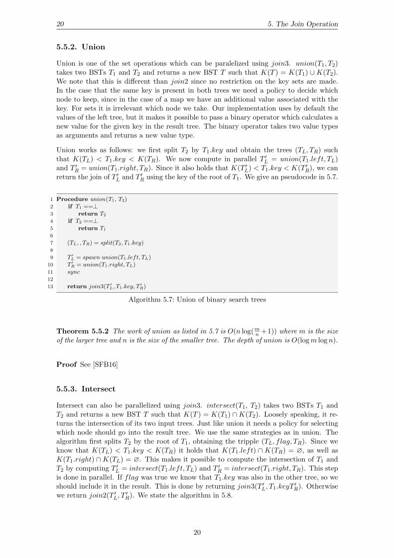
5.5.2. Union

Union is one of the set operations which can be paralelized using join3. union(T1, T2)takes two BSTs T1 and T2 and returns a new BST T such that K(T ) = K(T1) ∪K(T2).We note that this is different than join2 since no restriction on the key sets are made.In the case that the same key is present in both trees we need a policy to decide whichnode to keep, since in the case of a map we have an additional value associated with thekey. For sets it is irrelevant which node we take. Our implementation uses by default thevalues of the left tree, but it makes it possible to pass a binary operator which calculates anew value for the given key in the result tree. The binary operator takes two value typesas arguments and returns a new value type.

Union works as follows: we first split T2 by T1.key and obtain the trees (TL, TR) suchthat K(TL) < T1.key < K(TR). We now compute in parallel T ′

L = union(T1.left, TL)and T ′

R = union(T1.right, TR). Since it also holds that K(T ′L) < T1.key < K(T ′

R), we canreturn the join of T ′

L and T ′R using the key of the root of T1. We give an pseudocode in 5.7.

1 Procedure union(T1, T2)2 if T1 ==⊥3 return T2

4 if T2 ==⊥5 return T1

6

7 (TL, , TR) = split(T2, T1.key)8

9 T ′L = spawn union(T1.left, TL)10 T ′R = union(T1.right, TL)11 sync12

13 return join3(T ′L, T1.key, T′R)

Algorithm 5.7: Union of binary search trees

Theorem 5.5.2 The work of union as listed in 5.7 is O(n log(mn +1)) where m is the sizeof the larger tree and n is the size of the smaller tree. The depth of union is O(logm log n).

Proof See [SFB16]

5.5.3. Intersect

Intersect can also be parallelized using join3. intersect(T1, T2) takes two BSTs T1 andT2 and returns a new BST T such that K(T ) = K(T1) ∩K(T2). Loosely speaking, it re-turns the intersection of its two input trees. Just like union it needs a policy for selectingwhich node should go into the result tree. We use the same strategies as in union. Thealgorithm first splits T2 by the root of T1, obtaining the tripple (TL, f lag, TR). Since weknow that K(TL) < T1.key < K(TR) it holds that K(T1.left) ∩ K(TR) = ∅, as well asK(T1.right) ∩K(TL) = ∅. This makes it possible to compute the intersection of T1 andT2 by computing T ′

L = intersect(T1.left, TL) and T ′R = intersect(T1.right, TR). This step

is done in parallel. If flag was true we know that T1.key was also in the other tree, so weshould include it in the result. This is done by returning join3(T ′

L, T1.keyT′R). Otherwise

we return join2(T ′L, T

′R). We state the algorithm in 5.8.

20

5.5. Operations using Join 21

1 Procedure intersect (T1, T2)2 if T1 ==⊥3 return ⊥4 if T2 ==⊥5 return ⊥6

7 (TL, r, TR) = split(T2, T1.key)8

9 T ′L = spawn intersect(T1.left, TL)10 T ′R = intersect(T1.right, TL)11 sync12

13 if r == true14 return join3(T ′L, T1.key, T

′R)

15 else16 return join2(T ′L, T

′R)

Algorithm 5.8: Intersection of binary search trees

Theorem 5.5.3 The work of intersect as listed in 5.8 is O(n log(mn + 1)) where m isthe size of the larger tree and n is the size of the smaller tree. The depth of intersect isO(logm log n).

Proof See [SFB16].

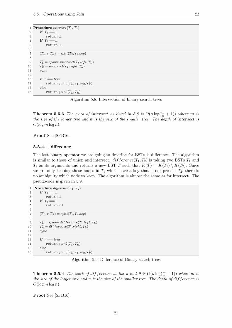
5.5.4. Difference

The last binary operator we are going to describe for BSTs is difference. The algorithmis similar to those of union and intersect. difference(T1, T2) is taking two BSTs T1 andT2 as its arguments and returns a new BST T such that K(T ) = K(T1) \K(T2). Sincewe are only keeping those nodes in T1 which have a key that is not present T2, there isno ambiguity which node to keep. The algorithm is almost the same as for intersect. Thepseudocode is given in 5.9.

1 Procedure difference(T1, T2)2 if T1 ==⊥3 return ⊥4 if T2 ==⊥5 return T16

7 (TL, r, TR) = split(T2, T1.key)8

9 T ′L = spawn difference(T1.left, TL)10 T ′R = difference(T1.right, TL)11 sync12

13 if r == true14 return join2(T ′L, T

′R)

15 else16 return join3(T ′L, T1.key, T

′R)

Algorithm 5.9: Difference of Binary search trees

Theorem 5.5.4 The work of difference as listed in 5.9 is O(n log(mn + 1)) where m isthe size of the larger tree and n is the size of the smaller tree. The depth of difference isO(logm log n).

Proof See [SFB16].

21

22 5. The Join Operation

5.5.5. Insert

Insertion can also be realized with the use of join3. If we want to insert a new key k intoT we first split T into TL and TR by k, and then join them back using k as the middlekey. The pseudocode is given in 5.10.

1 Procedure insert (T , k)2 (TL, f lag, TR) = split(T, k).3 return join3(TL, k, TR).

Algorithm 5.10: Insertion into Binary search trees

5.5.6. Delete

Removing an entry with a given key k from a BST is done similary to inserting. We firstsplit the tree T into TL and TR by k, but instead of calling join3 we call join2 in orderto merge the trees back.

1 Procedure delete(T , k)2 (TL, f lag, TR) = split(T, k).3 return join2(TL, TR).

Algorithm 5.11: Deletion from binary search trees

5.5.7. Range

Range accepts two keys as its arguments klow and khigh and returns a new tree containingall nodes with keys between klow and khigh. Depending on the implementation klow andkhigh can be included or not. For clearity, the pseudo code we describe in 5.12 does notinclude the boundary keys.

1 Procedure range(T , klow, khigh)2 (TL, f lag, TR) = split(T, klow).3 (T ′L, f lag

′, T ′R) = split(TR, khigh)4

5 return T ′L

Algorithm 5.12: Range on Binary search trees

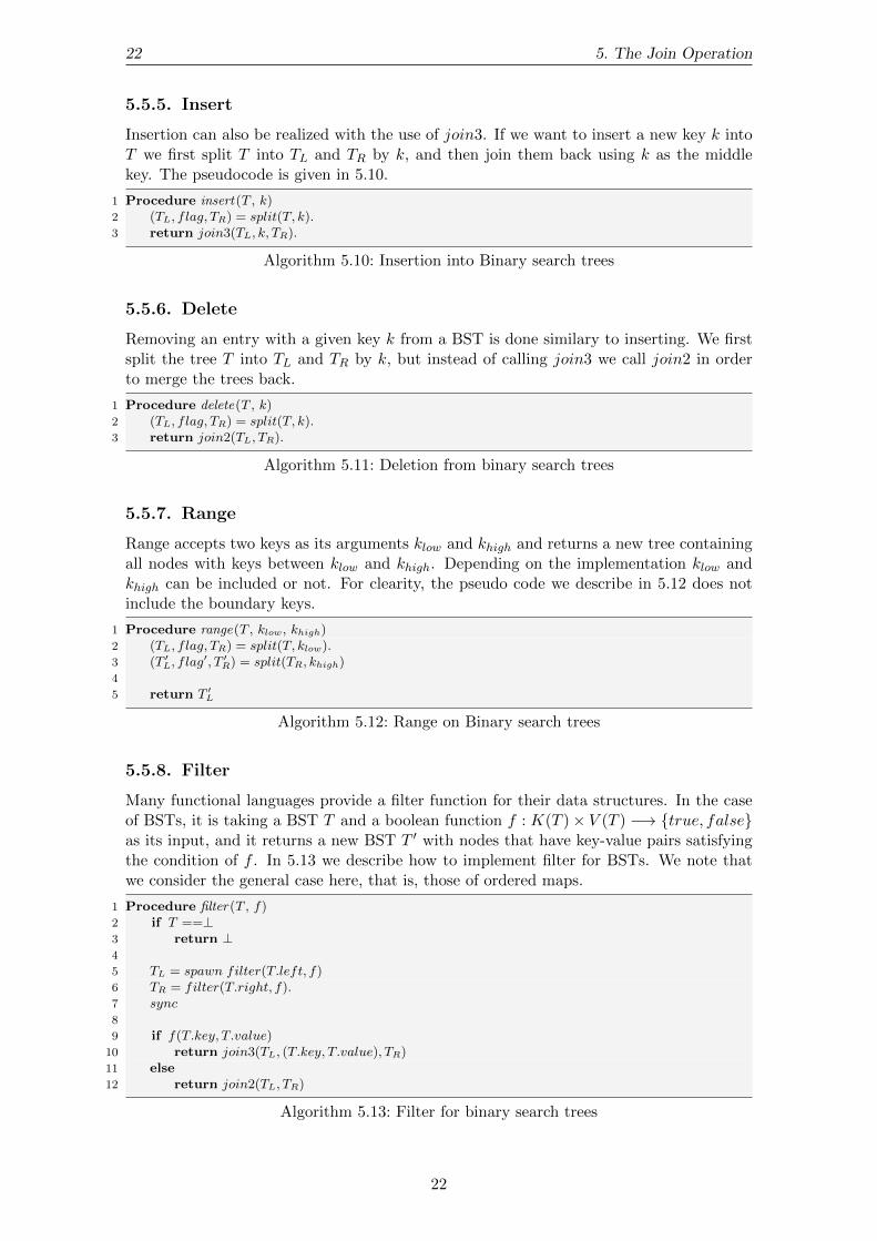
5.5.8. Filter

Many functional languages provide a filter function for their data structures. In the caseof BSTs, it is taking a BST T and a boolean function f : K(T )× V (T ) −→ true, falseas its input, and it returns a new BST T ′ with nodes that have key-value pairs satisfyingthe condition of f . In 5.13 we describe how to implement filter for BSTs. We note thatwe consider the general case here, that is, those of ordered maps.

1 Procedure filter (T , f)2 if T ==⊥3 return ⊥4

5 TL = spawn filter(T.left, f)6 TR = filter(T.right, f).7 sync8

9 if f(T.key, T.value)10 return join3(TL, (T.key, T.value), TR)11 else12 return join2(TL, TR)

Algorithm 5.13: Filter for binary search trees

22

5.5. Operations using Join 23

Theorem 5.5.5 The work of filter as listed in 5.13 is O(n) where n is the number ofnodes in the tree. The depth of filter is O((log n)2).

5.5.9. Build

Building a BST from an array of keys can be achieved in different ways. One way to builda BST is to insert each key one by one into the tree, yielding a complexity of O(n log n).Another way to build a BST is to make use of union, as described in 5.14. We note thatthis recursive algorithm even works if the array of keys is not sorted. In the general casethe running time of 5.14 is also O(n log n), but if the array of keys is already sorted therunning time becomes O(n). If we assume that the input array is already sorted, we canreplace the union call with a join3, by always taking the middle key of the current arrayas the middle key for join3. This also leads to a complexity of O(n), however with a lowerconstant. We give an exaple of the build variant for presorted keys in 5.15.

1 Procedure build (k1, ..., kn)2 if n == 03 return ⊥4 if n == 15 return new Node(k)6

7 TL = spawn build(k1, ..., kbn2 c)8 TR = build(kbn2 c+1, ..., kn)9 sync

10

11 return union(TL, TR)

Algorithm 5.14: Building binary search trees

Theorem 5.5.6 The work of build as listed in 5.14 is O(n log n) where n is the numberof keys to build a tree from. The depth of build is O((log n)3).

1 Procedure buildSorted (k1, ..., kn)2 if n == 03 return ⊥4 if n == 15 return new Node(k)6

7 m =⌊n2

⌋8 TL = spawn buildSorted(k1, ..., km−19 TR = buildSorted(km+1, ..., kn)

10 sync11

12 return join3(TL, km, TR)

Algorithm 5.15: Building binary search trees from a presorted sequence

Theorem 5.5.7 The work of buildSorted as listed in 5.15 is O(n) where n is the numberof keys to build a tree from. The depth of buildSorted is O(log n).

23

6. Implementation Details

6.1. Our library

We designed and implemented a library for ordered sets and maps around the join opera-tion. The implementation was done in C++. For each BBST we only had to implementthe join3 primitive in order to support the other operations mentioned in Chapter 5. Inour experiments we compared the performance of the different trees with each other. TheAVL tree turned out to be the best choice, but only by a small amount. We decided tofix the AVL tree for our containers, since allowing the user to provide a tree as additionaltemplate argument would lead to less readable code. A more complete overview of thelibrary interface is described in Chapter 7, while in the following we talk more about imple-mentation relevant details. Some features worth noting are that our library is persistent,parallel and concurrent.

The concurrency of our library is a side effect of the persistence and differs from concur-rent access in the traditional sense. Inserting n elements concurrently into an empty mapproduces in our case n distinct maps, each with one element. As opposed to common con-currenct search trees, where all elements are inserted into the same map. For parallelismwe use Intel’s Cilk-Plus extension for C++, which makes it possible to express dynamicnested parallelism for shared memory. To achieve confluently persistent data structureswe use a path copying approach, which is also used in many functional languages. Wenote that having full persistence is not enough in our case, since set operations like unioneffectively meld different data structure versions together. In conjunction with path copy-ing we use a referene counting scheme. Each node stores a reference count which denotesto how many objects it belongs to. This can be useful in multiple ways as we will seelater. A problem which arises is that of allocating new nodes and deleting nodes which donot belong to a tree anymore. This is because our aggregate set operations allocate andfree memory from multiple threads simultaneously. The conventional memory allocationmechanisms of C++ (new and delete) were not designed for this setting and scale verypoorly. The reason for this is that they lock the heap on each call. We tested severalscalable memory allocators (hoard and Intel’s tbb) which were available, but did notget too good results either. For this reason we implemented our own shared memory al-locator with garbage collection. In the next section we will describe how we made ourdata structures persistent. Following that, in section 6.3, we talk more about the memorymanagement of our library.

25

26 6. Implementation Details

6.2. Persistence

What we want from persistence is to retain BSTs across various operations on them. Thatis, inserting elements into an existing tree T should produce a new tree T ′ but withoutdestroying the old tree T . Similary, taking the union of two trees should produce a newtree without having any visible effect on the input trees. One way to achieve persistence isto copy the entire input trees before an operation and apply the operation on the copies.This however can be more costly than the operation being performed. Inserting into atree wouldn not take O(log n) time but O(n).

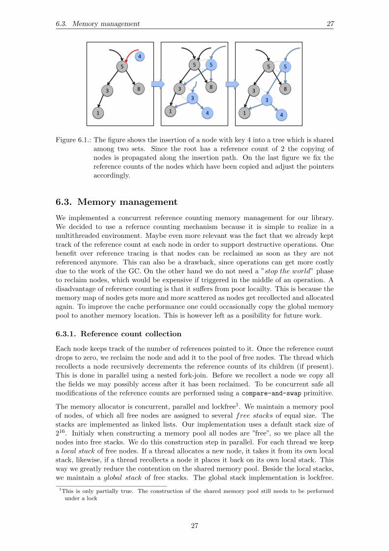
One way to improve the idea of copying the whole input is to only create copies alongthe modification path(s) of an operation. This approach is usually called path copying.By doing so we only copy those nodes which would have otherwise been modified by anoperation. Nodes which are adjacent to the modification path will be pointed to by theirold parent nodes as well as the newly created copy. This leads to the fact that largeparts of the input tree(s) are going to be shared with the created result tree. Figure 6.1illustrates an example of path copying in the case of insert. Since nodes can be sharedacross multiple trees, we keep track of a reference count at each node. This is necessary,since our garbage collection needs to know when it is safe to reclaim a node. This is notthe only benefit, however. Depending on the reference count of a node we distinguishbetween 3 actions:

• Reference count = 0 – node does not belong to any tree; it is safe to reclaim it bythe garbage collection. As the node is recollected, the reference counts of its childrenare decreased recursively.

• Reference count = 1 – node belongs to only one tree. If we detect this during anoperation we can safely use in-place updates instead of creating copies – destructiveoperations.

• Reference count ≥ 2 – node belongs to more than one tree. If we detect such anode during an operation we have to create a copy of it, otherwise we would be alsomodifying a tree which was not meant to be part of the operation. The copy initialyhas a reference count of 1 (it belongs to the result tree). The reference counts of itschildren are increased accordingly. This way we ensure that once we detect a sharednode, the whole subtree must also be shared.

Making any tree operation persistent becomes very simple. The only thing we have todo before we start modifying a tree is to increase the reference count of its root. Thiswill trigger the path copying right from the root of the tree and copy all nodes which areaffected by the operation. The reference counts also give us the freedom to actively choosewhether we want to use persistence or in-place (destructive) updates. Not increasingthe reference count before an operation would modify the tree destructively as much aspossible. That is, until it detects a node which is shared with another tree. From thatpoint on a path copying would be performed. Being able to perform both persistent anddestructive operations is useful, since the later one are more performant. To see how costlythe path copying really is, we performed an experiment with both versions. The resultscan be found in Chapter 8. Our library makes it possibe to choose between persistanceand destructive updates. It provides an final wrapper for this case, which we describe inChapter 7.

26

6.3. Memory management 27

5

3 8

1

5

3

5

3 8

1 4

5

3 8

1

5

3

4

4

Figure 6.1.: The figure shows the insertion of a node with key 4 into a tree which is sharedamong two sets. Since the root has a reference count of 2 the copying ofnodes is propagated along the insertion path. On the last figure we fix thereference counts of the nodes which have been copied and adjust the pointersaccordingly.

6.3. Memory management

We implemented a concurrent reference counting memory management for our library.We decided to use a refernce counting mechanism because it is simple to realize in amultithreaded environment. Maybe even more relevant was the fact that we already kepttrack of the reference count at each node in order to support destructive operations. Onebenefit over reference tracing is that nodes can be reclaimed as soon as they are notreferenced anymore. This can also be a drawback, since operations can get more costlydue to the work of the GC. On the other hand we do not need a ”stop the world” phaseto reclaim nodes, which would be expensive if triggered in the middle of an operation. Adisadvantage of reference counting is that it suffers from poor locailty. This is because thememory map of nodes gets more and more scattered as nodes get recollected and allocatedagain. To improve the cache performance one could occasionally copy the global memorypool to another memory location. This is however left as a posibility for future work.

6.3.1. Reference count collection

Each node keeps track of the number of references pointed to it. Once the reference countdrops to zero, we reclaim the node and add it to the pool of free nodes. The thread whichrecollects a node recursively decrements the reference counts of its children (if present).This is done in parallel using a nested fork-join. Before we recollect a node we copy allthe fields we may possibly access after it has been reclaimed. To be concurrent safe allmodifications of the reference counts are performed using a compare-and-swap primitive.

The memory allocator is concurrent, parallel and lockfree1. We maintain a memory poolof nodes, of which all free nodes are assigned to several free stacks of equal size. Thestacks are implemented as linked lists. Our implementation uses a default stack size of216. Initialy when constructing a memory pool all nodes are ”free”, so we place all thenodes into free stacks. We do this construction step in parallel. For each thread we keepa local stack of free nodes. If a thread allocates a new node, it takes it from its own localstack, likewise, if a thread recollects a node it places it back on its own local stack. Thisway we greatly reduce the contention on the shared memory pool. Beside the local stacks,we maintain a global stack of free stacks. The global stack implementation is lockfree.

1This is only partially true. The construction of the shared memory pool still needs to be performedunder a lock

27

28 6. Implementation Details

We use a double-word-compare-and-swap (16B) primitive on the head-pointer and itsversion number in order to avoid common concurrency pitfalls such as the ABA problemand memory corrucption. We also tested a version with hazard pointers, as described in[Mic04a]. Both of them compared equaly good.

Let s denote the maximum size of a free stack. If the local stack of a thread gets emptyit pulls a new stack of nodes from the global stack. However, if the local stack reachesthe size of 2s, we cut the stack in two and place one half back into the global stack. Thisway we ensure that after we acess the global stack by a thread, at least s allocations orrecollections need to be done till the next access. If the global stack runs out of memory,the first thread detecting it will initiate the construction of a new memory pool. New freestacks will be constructed in parallel and placed into the global stack. This is the only timea thread can actually block during an operation. However, as other threads repeatedlypull for new stacks while the global stack is being refilled, the allocator provides reasonablescalability even in this scenario.

28

7. Library Interface

Our library offers two kinds of ordered maps and one ordered set, all of which are persistentand safe for concurency:

• tree_map<K, V>

• tree_set<K>

• augmented_map<K, V, Op>

where K denotes the key type, V the value type for maps, and Op a binary operator takingtwo value types, and returning a value type. The generic types were expressed using C++’stemplates. The augmented map differs from the common ordered map by accepting anadditional binary operator. Each node of an augmented map stores the application of thebinary operator on the values of the tree rooted at itself. This can be an useful feature inmany applications. In table 7.1 we list the core functions supported by all of our containersalong with their cost.

Function Work, Depth

insert, delete, find log n

union, intersect, difference n log(mn + 1), log2 n

forall* n, log n

acumulate* log n

filter n, log2 n

build n log n, log3 n

split, range log n

next, previous, first, last log n

rank, select log n

Table 7.1.: The core functions in our map and set library and their asymptotic costs in big-O notation. acumulate is only supported by augmented maps, while forall

only by tree maps.

29

30 7. Library Interface

7.1. Method Summary

We will not go in much detail explaining each function in table 7.1. Most of them werealready introduced in Chapter 5 in the setting of BSTs. All functions except union,intersect and difference (and final) are member functions. Functions always returntheir result, however for the different containers some of the functions return a differentresult type. For example, map insertion returns a new map, but the set insertion returns anew set. In the the following we describe some of the functions from table 7.1, along withfunctions we did not mention. For clarity the descripton will refer to the map variants offunctions.

assigment operator (m1 = m2) – is performed in O(1) time. The reference count of theroot of m2 is increased by one. A new pointer to it is passed to m1, but prior tothat we invoke clear (see below) on m1.

m.content(out_iterator) – accepts an output iterator and appends all map entries toit. The resulting sequence is sorted in an ascending key order.

m.forall(f) – takes a function f : V → Vnew, and returns a new map where each valuev of the old map is replaced by f(v). We note that Vnew can also be a different datatype from V . Since sets do not have values stored in their nodes, we do not provide aforall method for sets. We also choose not to add it to the interface of augmentedmaps. The reason for this is the additional binary operator of augmented maps.Changing the value type of a map by forall would make the old binary operatormeaningles.

m.acumulate(k) – only supported by augmented maps. Takes a key k and returns theapplication of the map specific binary operator on all values whose entries have akey less or equal than k.

m.filter(f) – takes a boolean function f : K×V → true, false and returns a new mapwith all entries satisfying f . The key-value pairs are expressed using the std::pairtype.

m.split(k) – takes a key k and returns a pair of maps. The first map contains all entrieswith keys comparing less than k, while the second map contains all entries with keysgreater than k. The result is returned as a std::pair of maps.

m.range(l, r) – takes two keys l and r and returns a new map containing all entrieswith keys in the interval [l, r].

final(m) – can be used as a wrapper for maps. Functions accepting a map wrapped withfinal will operate destructively on the map.

map_union(m1, m2), map_intersect(m1, m2), map_difference(m1, m2) – take two mapsas arguments and return a new map which represents the union, intersection and dif-ference respectively. Can be used in conjuction with the final wrapper. Wrapping amap argument with final tells the function to perform the operation destructively.We achieve this by not increasing the reference count before the operation starts. Forexample, m = map_union(final(a), b) will destroy the first map, but the secondmap will remain unaffected by the operation.

m.clear() – empties the map. All nodes owned solely by the map are recollected bygarbage collecting threads. The collection is done in parallel using a nested fork-join.

tree_map<K, V>::init() – used to initialize the memory allocator. Needs to be calledonce at the program start before any other operation has been performed.

30

7.1. Method Summary 31

tree_map<K, V>::reserve(n) – accepts a number n and allocates space for n additionalnodes. The allocation is concurrenct safe and done in parallel. The function call isalso non-blocking – the allocation is performed asynchronously to the program flow.Unlike init, calling this function can also be ommited. If the memory allocator runsout of memory it will allocate a predefined amount of space automatically.

tree_map<K, V>::finish() – counterpart of init. Destroys the memory allocator andreturns all the reserved memory to the operating system.

One thing worth noting is that the memory allocator is not bound to individual objects,as it’s commonly implemented. It’s bound to a whole class instance. This is due to thefact that nodes are shared among multiple maps and sets. For this reason init, reserveand finish are implemented as static methods.

The maybe<T> type

Some of our functions may or may not return a valid result. In the case of maps, findaccepts a key k and only if k is present in the map it returns the value associated withit. But what should find return if no such key was present? For this reason we imple-mented a generic maybe type which wraps its result. The maybe object is convertible toa boolean, and as such it indicates whether it contains a valid value or not. To access avalue wrapped inside a maybe we use the star operator (*).

31

8. Evaluation

To test our library we performed several experiments, both sequential and parallel. Thisincludes comparing various functions and the join based BBST implementations with eachother. We also compare our library to the STL implemenations of ordered sets and maps,as well as their generic implementation of set_union. Since the STL only offers sequentialimplementations, we could not use it for any parallel experiments. To see how well ourlibrary performs against other parallelized search trees, we compared it against severalavailable implementations, including: MCSTL’s red black trees [FS07], weight-balancedB-trees [EKS14] and (a, b)-trees [AS15].

8.1. Setting

For our experiments we use a 64-core machine with 4 x AMD Opteron(tm) Processor 6278(16 cores, 2.4GHz, 1600MHz bus and 16MB L3 cache). The library was compiled using theg++ 4.8 version with the Cilk-Plus extension for nested paralleism. The only compilationflag we used was the -O2 flag. For testing purposes we choose our tree_map, but we notethat our tree_set and augmented_map would lead to similar results. To construct themaps in our experiments we generate multiple sets of key-value pairs varying in size from104 to 108. All keys and values are 32-bit unsigned integers choosen uniformly at random.In a single data set the keys are required to be unique, whereas the same value may occurmultiple times. In all of our experiments, for union, intersect and difference, n willdenote the size of the larger tree, while m will denote the size of the smaller tree.

8.2. Comparing different trees

To compare the various BBSTs we choose union as the representative operation. Otheroperations would lead to similar results since all operations except join3 are generic acrossthe trees. The experiments we performed showed that the trees are competitive with eachother. This may be due to the fact that the cost of cache misses dominates over theother operations we perform. Despite the similarities, the AVL tree gave the overall bestresults. It is about 15% better than the red black tree, which had the slowest times in ourexperiments. Table 8.1 shows the timings of all our BBSTs across different thread countsfor n = m = 108, while table 8.2 shows the results for n = 108 and m = 107. It is evidentthat our union algorithm performs work proportional to the smaller input tree.

33

34 8. Evaluation

TreeNumber of Threads

1 2 4 8 16 32 64

AVL 34.69 17.75 8.86 4.51 2.29 1.17 0.80

WB 35.37 18.30 9.40 4.79 2.41 1.23 0.87

Treap 37.35 19.40 10.03 5.08 2.57 1.30 0.86

RB 40.91 21.02 10.85 5.54 2.79 1.41 0.97

Table 8.1.: Timings for union across different trees (n = m = 108).

TreeNumber of Threads

1 2 4 8 16 32 64

AVL 3.37 1.75 0.91 0.46 0.23 0.12 0.085

WB 3.60 1.85 0.94 0.49 0.24 0.12 0.089

Treap 3.71 1.95 1.01 0.50 0.25 0.13 0.088

RB 4.46 2.19 1.14 0.55 0.28 0.14 0.1

Table 8.2.: Timings for union across different trees (n = 108,m = 107).

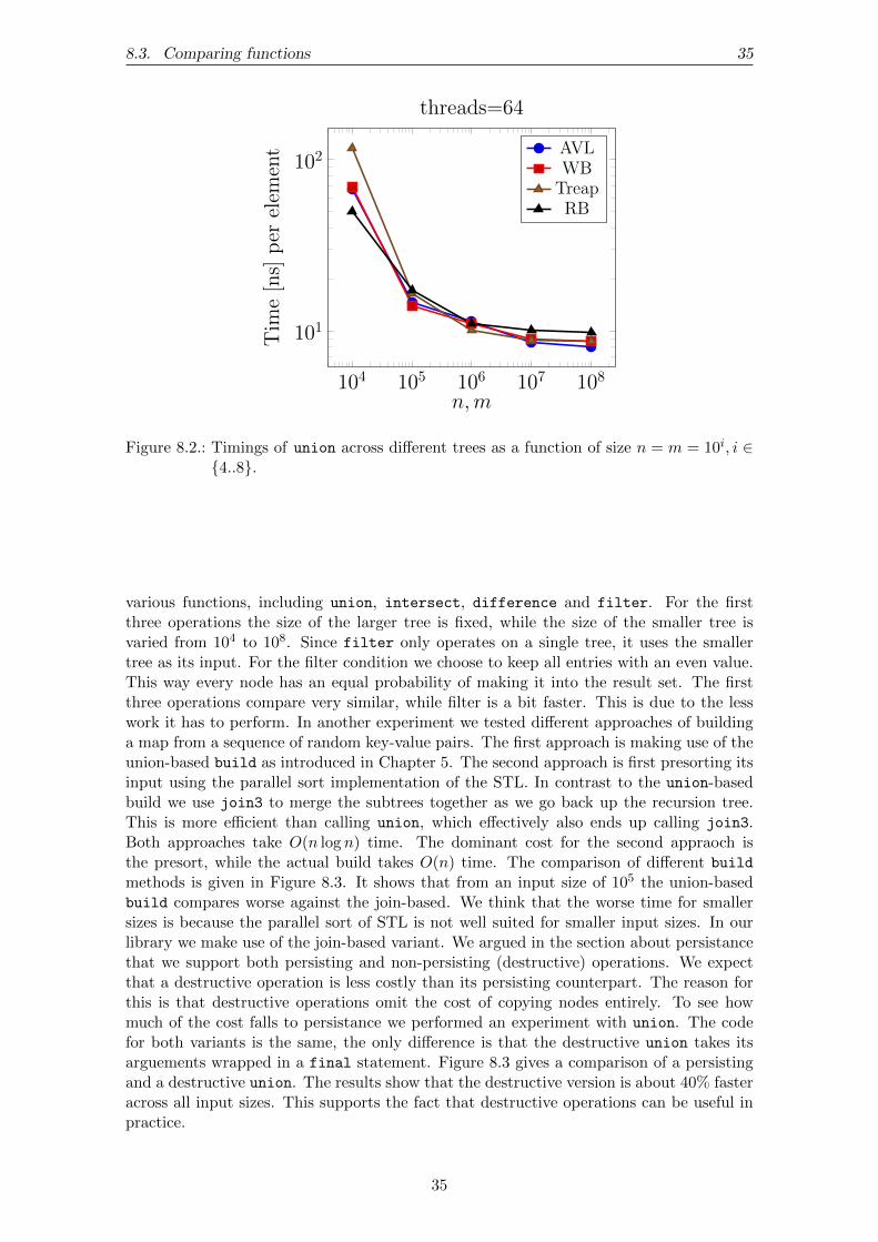
In Figure 8.1 we show the speedup of union across different trees for n = m = 108. Weget a 40-fold speedup on our machine. For smaller input trees we get less speed up, whichis due to the lack of paralelism. In the case of n = m = 105 we get a speedup of 25. Figure8.2 illustrates the timings of union as a function of size where n = m = 10i.

0 20 40 60

0

20

40

60

Threads

Speedup

Union, n = m = 108

AVLRB

TreapWB

Figure 8.1.: Speed up for union across different trees (n = m = 108).

8.3. Comparing functions

We use the AVL tree as the representative tree to compare different functions with eachother. As one can see from the previous experiments, choosing any other tree wouldnot have a significant impact on our timings. In Figure 8.3 we give a comparison of

34

8.3. Comparing functions 35

104 105 106 107 108

101

102

n,m

Tim

e[ns]per

elem

ent

threads=64

AVLWBTreapRB

Figure 8.2.: Timings of union across different trees as a function of size n = m = 10i, i ∈4..8.

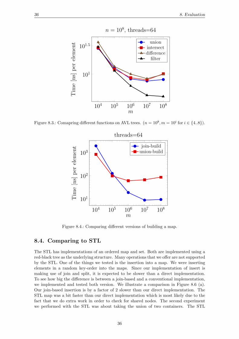
various functions, including union, intersect, difference and filter. For the firstthree operations the size of the larger tree is fixed, while the size of the smaller tree isvaried from 104 to 108. Since filter only operates on a single tree, it uses the smallertree as its input. For the filter condition we choose to keep all entries with an even value.This way every node has an equal probability of making it into the result set. The firstthree operations compare very similar, while filter is a bit faster. This is due to the lesswork it has to perform. In another experiment we tested different approaches of buildinga map from a sequence of random key-value pairs. The first approach is making use of theunion-based build as introduced in Chapter 5. The second approach is first presorting itsinput using the parallel sort implementation of the STL. In contrast to the union-basedbuild we use join3 to merge the subtrees together as we go back up the recursion tree.This is more efficient than calling union, which effectively also ends up calling join3.Both approaches take O(n log n) time. The dominant cost for the second appraoch isthe presort, while the actual build takes O(n) time. The comparison of different build

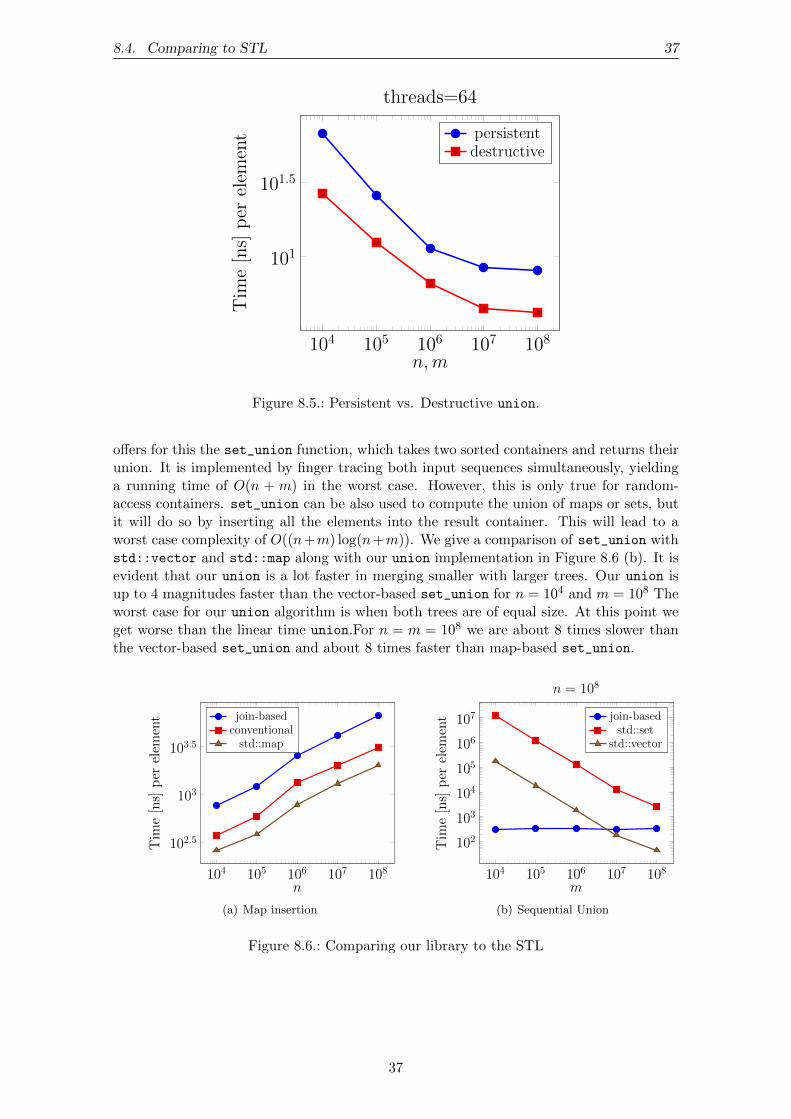
methods is given in Figure 8.3. It shows that from an input size of 105 the union-basedbuild compares worse against the join-based. We think that the worse time for smallersizes is because the parallel sort of STL is not well suited for smaller input sizes. In ourlibrary we make use of the join-based variant. We argued in the section about persistancethat we support both persisting and non-persisting (destructive) operations. We expectthat a destructive operation is less costly than its persisting counterpart. The reason forthis is that destructive operations omit the cost of copying nodes entirely. To see howmuch of the cost falls to persistance we performed an experiment with union. The codefor both variants is the same, the only difference is that the destructive union takes itsarguements wrapped in a final statement. Figure 8.3 gives a comparison of a persistingand a destructive union. The results show that the destructive version is about 40% fasteracross all input sizes. This supports the fact that destructive operations can be useful inpractice.

35

36 8. Evaluation

104 105 106 107 108

101

101.5

m

Tim

e[ns]per

elem

ent

n = 108, threads=64

unionintersectdifference

filter

Figure 8.3.: Comapring different functions on AVL trees. (n = 108,m = 10i for i ∈ 4..8).

104 105 106 107 108

101

102

103

m

Tim

e[ns]per

elem

ent

threads=64

join-buildunion-build

Figure 8.4.: Comparing different versions of building a map.

8.4. Comparing to STL

The STL has implementations of an ordered map and set. Both are implemented using ared-black tree as the underlying structure. Many operations that we offer are not supportedby the STL. One of the things we tested is the insertion into a map. We were insertingelements in a random key-order into the maps. Since our implementation of insert ismaking use of join and split, it is expected to be slower than a direct implementation.To see how big the difference is between a join-based and a conventional implementation,we implemented and tested both version. We illustrate a comparison in Figure 8.6 (a).Our join-based insertion is by a factor of 2 slower than our direct implementation. TheSTL map was a bit faster than our direct implementation which is most likely due to thefact that we do extra work in order to check for shared nodes. The second experimentwe performed with the STL was about taking the union of two containers. The STL

36

8.4. Comparing to STL 37

104 105 106 107 108

101

101.5

n,m

Tim

e[ns]per

elem

ent

threads=64

persistentdestructive

Figure 8.5.: Persistent vs. Destructive union.

offers for this the set_union function, which takes two sorted containers and returns theirunion. It is implemented by finger tracing both input sequences simultaneously, yieldinga running time of O(n + m) in the worst case. However, this is only true for random-access containers. set_union can be also used to compute the union of maps or sets, butit will do so by inserting all the elements into the result container. This will lead to aworst case complexity of O((n+m) log(n+m)). We give a comparison of set_union withstd::vector and std::map along with our union implementation in Figure 8.6 (b). It isevident that our union is a lot faster in merging smaller with larger trees. Our union isup to 4 magnitudes faster than the vector-based set_union for n = 104 and m = 108 Theworst case for our union algorithm is when both trees are of equal size. At this point weget worse than the linear time union.For n = m = 108 we are about 8 times slower thanthe vector-based set_union and about 8 times faster than map-based set_union.

104 105 106 107 108

102.5

103

103.5

n

Tim

e[ns]per

elem

ent join-based

conventionalstd::map

(a) Map insertion

104 105 106 107 108

102

103

104

105

106

107

m

Tim

e[ns]per

elem

ent

n = 108

join-basedstd::set

std::vector

(b) Sequential Union

Figure 8.6.: Comparing our library to the STL

37

38 8. Evaluation

8.5. Comparing to parallel implementations

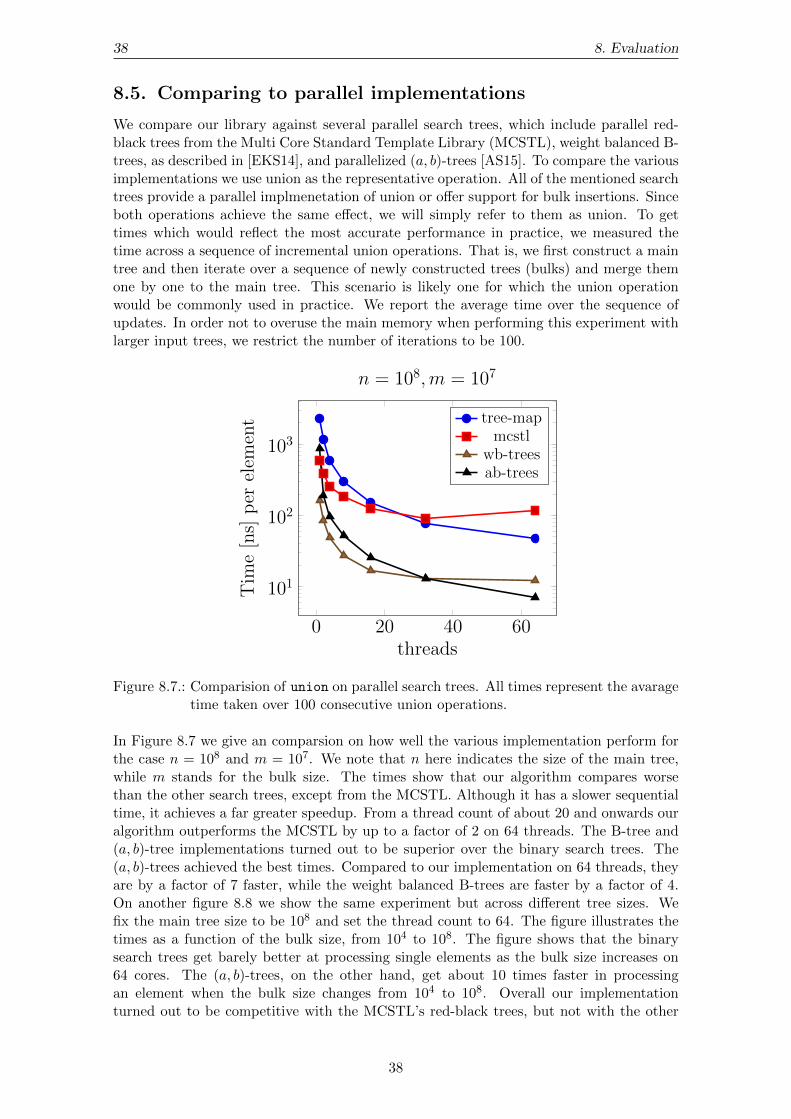
We compare our library against several parallel search trees, which include parallel red-black trees from the Multi Core Standard Template Library (MCSTL), weight balanced B-trees, as described in [EKS14], and parallelized (a, b)-trees [AS15]. To compare the variousimplementations we use union as the representative operation. All of the mentioned searchtrees provide a parallel implmenetation of union or offer support for bulk insertions. Sinceboth operations achieve the same effect, we will simply refer to them as union. To gettimes which would reflect the most accurate performance in practice, we measured thetime across a sequence of incremental union operations. That is, we first construct a maintree and then iterate over a sequence of newly constructed trees (bulks) and merge themone by one to the main tree. This scenario is likely one for which the union operationwould be commonly used in practice. We report the average time over the sequence ofupdates. In order not to overuse the main memory when performing this experiment withlarger input trees, we restrict the number of iterations to be 100.

0 20 40 60

101

102

103

threads

Tim

e[ns]per

elem

ent

n = 108,m = 107

tree-mapmcstl

wb-treesab-trees

Figure 8.7.: Comparision of union on parallel search trees. All times represent the avaragetime taken over 100 consecutive union operations.

In Figure 8.7 we give an comparsion on how well the various implementation perform forthe case n = 108 and m = 107. We note that n here indicates the size of the main tree,while m stands for the bulk size. The times show that our algorithm compares worsethan the other search trees, except from the MCSTL. Although it has a slower sequentialtime, it achieves a far greater speedup. From a thread count of about 20 and onwards ouralgorithm outperforms the MCSTL by up to a factor of 2 on 64 threads. The B-tree and(a, b)-tree implementations turned out to be superior over the binary search trees. The(a, b)-trees achieved the best times. Compared to our implementation on 64 threads, theyare by a factor of 7 faster, while the weight balanced B-trees are faster by a factor of 4.On another figure 8.8 we show the same experiment but across different tree sizes. Wefix the main tree size to be 108 and set the thread count to 64. The figure illustrates thetimes as a function of the bulk size, from 104 to 108. The figure shows that the binarysearch trees get barely better at processing single elements as the bulk size increases on64 cores. The (a, b)-trees, on the other hand, get about 10 times faster in processingan element when the bulk size changes from 104 to 108. Overall our implementationturned out to be competitive with the MCSTL’s red-black trees, but not with the other

38

8.5. Comparing to parallel implementations 39

104 105 106 107 108

101

102

m

Tim

e[ns]per

elem

ent

n = 108, threads=64

tree-map

mcstl

wb-trees

ab-trees

Figure 8.8.: Comparision of union on parallel search trees. All times represent the averagetime taken over 100 consecutive union operations.

implementations. Some reasons might include their high cache efficency, but also overalllower height compared to the binary search trees.

39

9. Conclusion

We implemented a parallel and persistent C++ library for ordered maps and sets. Forthe underlying structure we compared the performance of four different balanced binarysearch trees, including AVL trees, red-black trees, weight-balanced trees and treaps. Theimplementation of a single tree is fully captured by the join operation. We describe efficientjoin algorithms for all of our trees. They are work efficient and construct a balanced resulttree. With the use of only join we show how to implement many other tree operations.

Based on the experiments we performed our library achieves its best results with theAVL tree. Some reasons for this might be the stricter balacing condition and the simplerimplemenation. We demonstrated that the join-based algorithms for union, intersect anddifference can be up to several magnitudes faster (on a single core) in merging smaller withlarger trees, compared to a naive sequential implementation. However, our implementationdid not turn out to be the best option when it comes to the parallel setting. Despite beingcomparable to the MCSTL, our implementation was outperformed by weight-balancedB-trees and (a, b)-trees. Our parallel algorihms achieve a speedup of up to 44 on 64cores. On larger input files the speedup is almost linear when using less than 32 threads,beyond we achieve a parallel slowdown. We do not think that the reason for this is thelack of parallelism. It is more likely due to the memory communication, which seemsto be a bottleneck. Our implementation was designed to be persistent and concurrentsafe. Despite the additional work we do to achieve this, our implementation comparedreasonably well to the STL implementation of ordered sets and maps. Persistence can beuseful in many applications. We use a version of path copying which makes it possible touse to use persistence at will. We have shown that it can be useful in practice to supportdestructive operations as well. It would be interesting to see how our implementation wouldperform with other persistence techniques, which are more memory efficient. Anotherthing we left as a possibility for future work was the implementation of a tracing garbagecollector. It would improve the cache locality and reduce the time overhead of recollectingnodes immediately.

41

Bibliography

[AS15] Y. Akhremtsev and P. Sanders, “Fast parallel operations on search trees,” 2015.

[AVL62] G. M. Adelson-Velsky and E. M. Landis, “An algorithm for the organizationof informaiton,” Soviet Mathematics Doklady, 1962.

[BCCO10] N. Bronson, J. Casper, H. Chafi, and K. Olukotun, “A practical concurrentbinary search tree,”PPoPP ’10 Proceedings of the 15th ACM SIGPLAN Sym-posium on Principles and Practice of Parallel Programming, 2010.

[BE13] J. Besa and Y. Eterovic, “A concurrent red-black tree,” Journal of Parallel andDistributed Computing, 2013.

[BM80] N. Blum and K. Mehlhorn, “On the avarage number of rebalacing operationsin weight-balanced trees,” Theoretical Computer Science 11, 1980.

[BRM98] G. Blelloch and M. Reid-Miller, “Fast set operations using treaps,”10th AnnualACM Symposium on Parallel Algorithms and Architectures (SPAA’98), 1998.

[DSST89] J. R. Driscoll, N. Sarnak, D. D. Sleator, and R. E. Tarjan, “Making datastructures persistent,” Journal of Computer and System Sciences, 1989.

[EKS14] S. Erb, M. Kobitzsch, and P. Sanders, “Parallel bi-objective shortest pathsusing weight-balanced b-trees with bulk updates,” Proceedings of the 13th In-ternational Symposium on Experimental Algorithms, 2014.

[FK01] A. Fiat and H. Kaplan, “Making data structures confluently persistent,” Pro-ceedings of the 12th Annual Symposium on Discrete Algorithms, 2001.

[FS07] L. Frias and J. Singler, “Parallelization of bulk operations for stl dictionar-ies,” Proceeding Euro-Par’07 Proceedings of the 2007 conference on Parallelprocessing, 2007.

[GS78] L. Guibas and R. Sedgeweick, “A dichromatic framework for balanced trees,”Proceedings of the 19th Annual Conference on Foundations of Computer Sci-ence, 1978.

[JGB97] E. Johnson, D. Gannon, and P. Beckman, “Hpc++: Experiments with the par-allel standard template library*,” ICS ’97 Proceedings of the 11th internationalconference on Supercomputing, 1997.

[KL80] H. T. Kung and P. L. Lehman, “Concurrent manipulation of binary searchtrees,” ACM Transactions on Database Systems (TODS), 1980.

[Mic04a] M. M. Michael, “Hazard pointers: Safe memory reclamation for lock-free ob-jects,” IEEE Transactions on Parallel and Distributed Systems, 2004.

[Mic04b] ——, “Scalable lock-free dynamic memory allocation,” ACM SIGPLAN 2004,Conference on Programming Language Design and Implementation (PLDI),2004.

43

44 Bibliography

[NR72] J. Nievergelt and E. M. Reingold, “Binary search trees of bounded balance,”STOC ’72 Proceedings of the fourth annual ACM symposium on Theory ofcomputing, 1972.

[PP01] H. Park and K. Park, “Parallel algorithms for red–black trees,” TheoreticalComputer Science, 2001.

[SA96] R. Seidel and C. R. Aragon, “Randomized search trees,” Algorithmica, 1996.

[SFB16] Y. Sun, D. Ferizovic, and G. Blelloch, “Just join for parallel ordered sets andmaps,” 2016.

[ST86] N. Sarnak and R. E. Tarjan, “Planar point location using persistent searchtrees,” Communications of the ACM, 1986.

[Tar82] R. E. Tarjan, “Data structures and network algorithms,” SIAM, 1982.

44

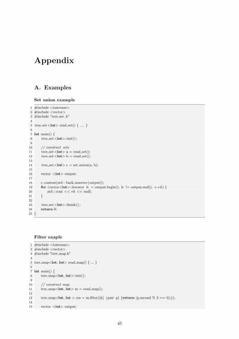
Appendix

A. Examples

Set union example

1 #include <iostream>2 #include <vector>3 #include ”tree set .h”4

5 tree set<int> read set() ... 6

7 int main() 8 tree set<int>::init() ;9

10 // construct sets11 tree set<int> a = read set();12 tree set<int> b = read set();13

14 tree set<int> c = set union(a, b);15

16 vector <int> output;17

18 c.content(std :: back inserter(output));19 for (vector<int>::iterator it = output.begin(); it != output.end(); ++it) 20 std :: cout << ∗it << endl;21 22

23 tree set<int>::finish() ;24 return 0;25

Filter exaple

1 #include <iostream>2 #include <vector>3 #include ”tree map.h”4

5 tree map<int, int> read map() ... 6

7 int main() 8 tree map<int, int>::init();9

10 // construct map11 tree map<int, int> m = read map();12

13 tree map<int, int > res = m.filter([&] (pair p) return (p.second % 2 == 0););14

15 vector <int> output;

45

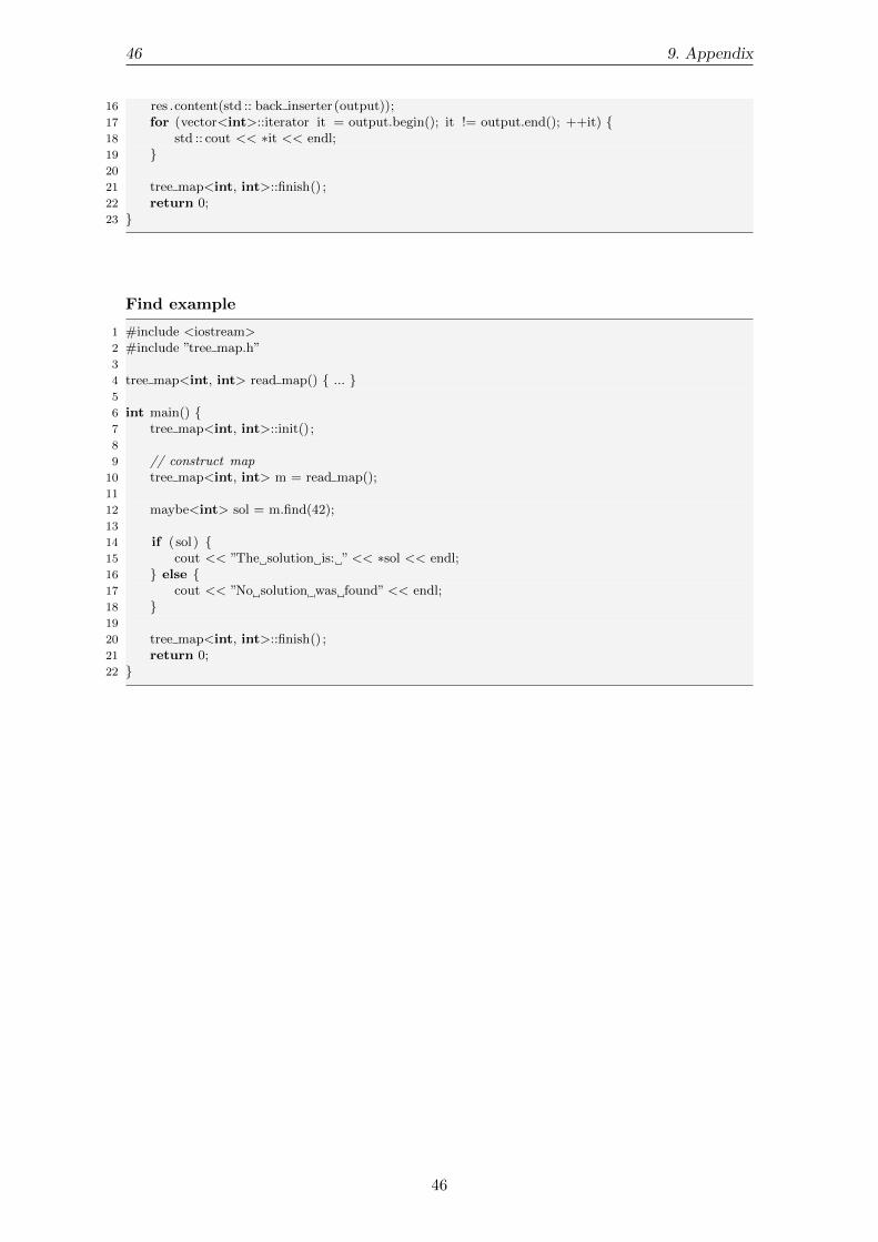
46 9. Appendix

16 res .content(std :: back inserter(output));17 for (vector<int>::iterator it = output.begin(); it != output.end(); ++it) 18 std :: cout << ∗it << endl;19 20

21 tree map<int, int>::finish() ;22 return 0;23

Find example

1 #include <iostream>2 #include ”tree map.h”3

4 tree map<int, int> read map() ... 5

6 int main() 7 tree map<int, int>::init();8

9 // construct map10 tree map<int, int> m = read map();11

12 maybe<int> sol = m.find(42);13

14 if ( sol ) 15 cout << ”The solution is: ”<< ∗sol << endl;16 else 17 cout << ”No solution was found”<< endl;18 19

20 tree map<int, int>::finish() ;21 return 0;22

46