a practical course in graphical bayesian modeling; class 1 eric-jan wagenmakers

A Practical Course in Graphical Bayesian Modeling; Class 1

Eric-Jan

Wagenmakers

Outline

A bit of probability theory Bayesian foundations Parameter estimation: A simple example WinBUGS and R2WinBUGS

Probability Theory (Wasserman, 2004)

The sample space Ω is the set of possible outcomes of an experiment.

If we toss a coin twice then Ω = {HH, HT, TH, TT}.

The event that the first toss is heads isA = {HH, HT}.


A B denotes intersection: “A and B”

denotes union: “A or B” A B


0P A

1P

1 1

i ii i

P A P A

P is a probability measure when the following axiomsare satisfied:

2. Probabilities add to 1.

1. Probabilities are never negative:

2. The probability of the union of non-overlapping (disjoint) events is its sum:


For any events A and B:

,P A B P A P B P A B

Ω

A B

Conditional Probability

The conditional probability of A given B is

,|

P A BP A B

P B

Ω

A B


You will often encounter this as

Ω

A B

| ,P A B P B P A B


, |P A B P A B P B

From

, |P A B P B A P A

and

follows Bayes’ rule.

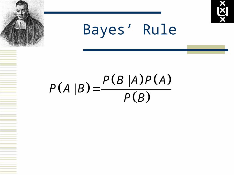
Bayes’ Rule

||

P B A P AP A B

P B

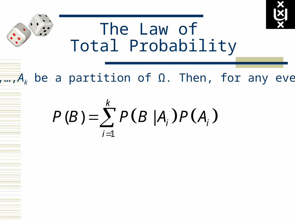
The Law of Total Probability

1

( ) |k

i ii

P B P B A P A

Let A1,…,Ak be a partition of Ω. Then, for any event B:

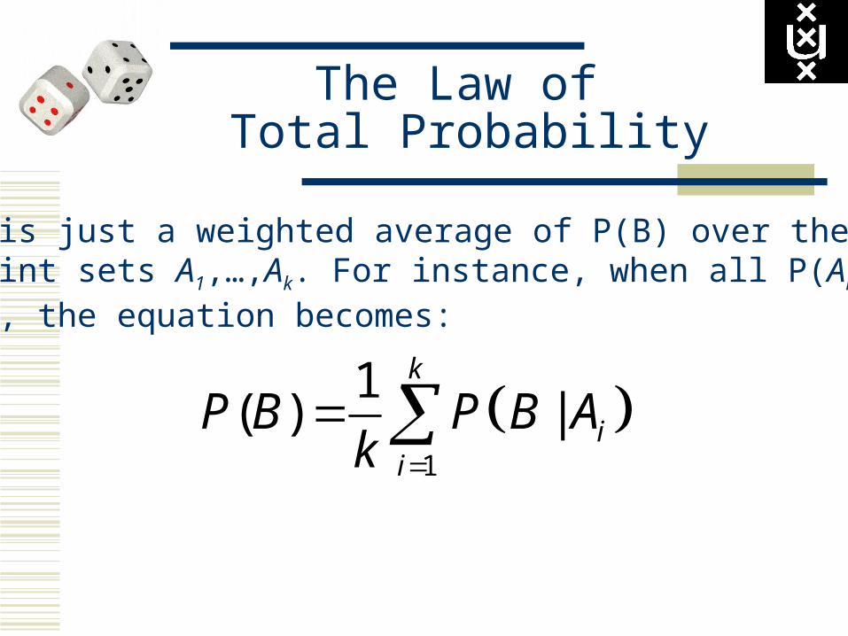
The Law of Total Probability

This is just a weighted average of P(B) over thedisjoint sets A1,…,Ak. For instance, when all P(Ai) areequal, the equation becomes:

1

1( ) |

k

ii

P B P B Ak

Bayes’ Rule Revisited

1

||

|

i ii k

i ii

P B A P AP A B

P B A P A

Example (Wasserman, 2004)

I divide my Email into three categories: “spam”, “low priority”, and “high priority”.

Previous experience suggests that the a priori probabilities of a random Email belonging to these categories are .7, .2, and .1, respectively.

Example (Wasserman, 2004)

The probabilities of the word “free” occurring in the three categories is .9, .01, .01, respectively.

I receive an Email with the word “free”. What is the probability that it is spam?

Outline


The Bayesian Agenda

Bayesians use probability to quantify uncertainty or “degree of belief” about parameters and hypotheses.

Prior knowledge for a parameter θ is updated through the data to yield the posterior knowledge.

The Bayesian Agenda

|

| |P D P

P D P D PP D

Also note that this equation allows one to learn, from the probability of what is observed, something about what isnot observed.

The Bayesian Agenda

But why would one measure “degree of belief” by means of probability? Couldn’t we choose something else that makes sense?

Yes, perhaps we can, but the choice of probability is anything but ad-hoc.

The Bayesian Agenda

Assume “degree of belief” can be measured by a single number.

Assume you are rational, that is, not self-contradictory or “obviously silly”.

Then degree of belief can be shown to follow the same rules as the probability calculus.

The Bayesian Agenda

For instance, a rational agent would not hold intransitive beliefs, such as:

Bel A Bel B

Bel B Bel C

Bel C Bel A

The Bayesian Agenda

When you use a single number to measure uncertainty or quantify evidence, and these numbers do not follow the rules of probability calculus, you can (almost certainly?) be shown to be silly or incoherent.

One of the theoretical attractions of the Bayesian paradigm is that it ensures coherence right from the start.

Coherence Examplea la De Finetti

There exists a ticket that says “If the French national soccer team wins the 2010 World Cup, this ticket pays $1.”

You must determine the fair price for this ticket. After you set the price, I can choose to either sell the

ticket to you, or to buy the ticket from you. This is similar to how you would divide a pie according to the rule “you cut, I choose”.

Please write this number down, you are not allowed to change it later!


There exists another ticket that says “If the Spanish national soccer team wins the 2010 World Cup, this ticket pays $1.”

You must again determine the fair price for this ticket.


There exists a third ticket that says “If either the French or the Spanish national soccer team wins the 2010 World Cup, this ticket pays $1.”

What is the fair price for this ticket?

Bayesian Foundations

Bayesians use probability to quantify uncertainty or “degree of belief” about parameters and hypotheses.

Prior knowledge for a parameter θ is updated through the data to yield posterior knowledge.

This happens through the use of probability calculus.

Bayes’ Rule

||

P D PP D

P D

Posterior Distribution

PriorDistribution

Likelihood

Marginal Probabilityof the Data

Bayesian Foundations

|

| |P D P

P D P D PP D

This equation allows one to learn, from the probability of what is observed, something about what isnot observed. Bayesian statistics was long known as “inverse probability”.

Nuisance Variables

Suppose θ is the mean of a normal distribution, and α is the standard deviation.

You are interested in θ, but not in α. Using the Bayesian paradigm, how can you go

from P(θ, α | x) to P(θ | x)? That is, how can you get rid of the nuisance parameter α? Show how this involves P(α).

Nuisance Variables

| ( , | )P x P x d ( | , ) |P x P x d ( | , ) |P x P x P d

Predictions

Suppose you observe data x, and you use a model with parameter θ.

What is your prediction for new data y, given that you’ve observed x? In other words, show how you can obtain P(y|x).

Predictions

| ( | , ) |P y x P y x P x d

Want to Know More?

Outline


Bayesian Parameter Estimation: Example

We prepare for you a series of 10 factual true/false questions of equal difficulty.

You answer 9 out of 10 questions correctly. What is your latent probability θ of

answering any one question correctly?


We start with a prior distribution for θ. This reflect all we know about θ prior to the experiment. Here we make a standard choice and assume that all values of θ are equally likely a priori.


We then update the prior distribution by means of the data (technically, the likelihood) to arrive at a posterior distribution.

The Likelihood

We use the binomial model, in which P(D|θ) is given by

where n =10 is the number of trials, and s=9 is the number of successes.

| 1n ssn

P Ds


The posterior distribution is a compromise between what we knew before the experiment (i.e., the prior) and what we have learned from the experiment (i.e., the likelihood). The posterior distribution reflects all that we know about θ.

Mode = 0.9

95% confidence interval: (0.59, 0.98)


Sometimes it is difficult or impossible to obtain the posterior distribution analytically.

In this case, we can use Markov chain Monte Carlo algorithms to sample from the posterior. As the number of samples increases, the approximation to the analytical posterior becomes arbitrarily small.

Mode = 0.89

95% confidence interval: (0.59, 0.98)

With 9000 samples, almost identical toanalytical result.

Outline


WinBUGS

Bayesian inference Using

Gibbs Sampling

You want to have thisinstalled (plus the registration key)

WinBUGS

Knows many probability distributions (likelihoods);

Allows you to specify a model; Allows you to specify priors; Will then automatically run the MCMC

sampling routines and produce output.

Want to Know MoreAbout MCMC?

Models in WinBUGS

The models you can specify in WinBUGS are directed acyclical graphs (DAGs).

Models in WinBUGS(Spiegelhalter, 1998)

A

B D

C E

Below, E depends only on C


A

B D

C E

If the nodes are stochastic, the jointdistribution factorizes…


A

B D

C E

P(A,B,C,D,E) = P(A) P(B) P(C|A,B) P(D|A,B) P(E|C)


A

B D

C E

This means we can sometimes perform“local” computations to get what we want


A

B D

C E

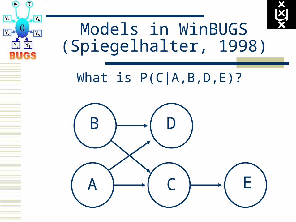
What is P(C|A,B,D,E)?


A

B D

C E

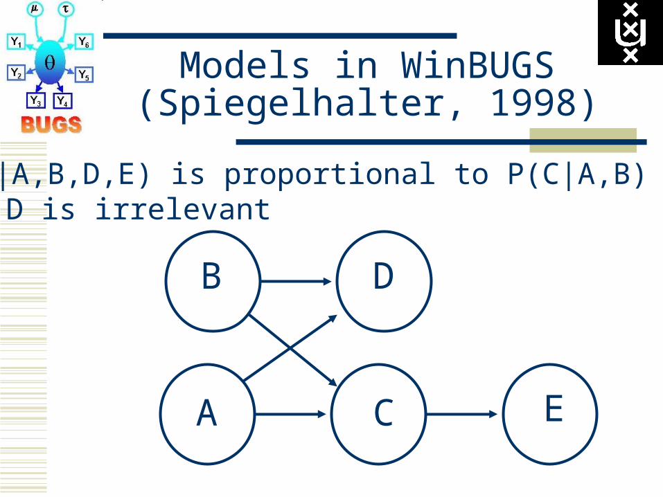
P(C|A,B,D,E) is proportional to P(C|A,B) P(E|C) D is irrelevant

WinBUGS & R

WinBUGS produces MCMC samples. We want to analyze the output in a nice

program, such as R. This can be accomplished using the R

package “R2WinBUGS”

End of Class 1

a practical course in graphical bayesian modeling; class 1 eric-jan wagenmakers

Documents