a practical and comparative study of call graph

IOSR Journal of Computer Engineering (IOSRJCE)

ISSN: 2278-0661 Volume 1, Issue 4 (May-June 2012), PP 14-26 www.iosrjournals.org

www.iosrjournals.org 14 | Page

A Practical and Comparative Study of Call Graph Construction

Algorithms

Sajad Ahmad Bhat, Dr. Jatender Singh

(Deptt. of computer science Manav harti Universiety Solan H.P)

(Principal/ Golden college of Engg. And Tech.)

ABSTRACT: A number of Call Graph construction algorithms have been designed for construction of Call

Graphs for object-oriented languages. Each of the Call Graph contraction algorithms were proposed to keep in

mind the improvements over previous Call Graphs in terms of precision, cost and accuracy. In object oriented

languages the Call Graphs are generally contracted to represent the calling relationship between the program’s

methods. The Call Graph forms the bases for deducing the information about the classes and the methods that are actually invoked, this information can be used to find call sites were virtual function calls can be replaced

by direct calls and inline-expansions can be put into work where ever possible. In this paper we present an

empirical comparison of various well known Call Graph construction algorithms. Here we used Scoot bytecode

reader as front-end to implement various Call Graph construction algorisms. In the processes Scoot bytecode

reader is used to read the bytecode of a specific java program then the reachable methods are found for each

invoked method. For storing information about the classes, methods, fields and statements we created our own

set of data structures.

Finally we tested and evaluated the developed algorithms with a variety of java benchmark programs

to gather the information for the comparison of various Call Graph algorithms which is the goal of this work.

We have included most of the Call Graph algorithms of popularity in this work. The main aim of the work is to

consider all the dimensions of the Call Graph construction algorithms like cost, precision, memory and time requirements for its construction. The previous works has either not included all the algorithms of fame or have

left some of their construction constraints untouched. This work will bring an effective empirical comparison to

the front and will help to reveal that which Call Graph construction algorithm is best and when. The results in

the work are mainly considered valid for java and other statically typed object-oriented languages.

I. INTRODUCTION The Call Graphs are the basic data structures to analyze the calling relationships between program

methods [1]. A Call Graph is generally a set of directed edges that connects the call sites to their corresponding

target methods. A Call Graph is a very powerful tool that can be used in a number ways like it can help in planning testing strategies, reducing the program size by eliminating the methods that are not invoked, helps

programmers to understand the nature of larger programs and dubbing etc. depending up on the static or

dynamic behavior of the program the Call Graphs can be static or dynamic. The dynamic Call Graphs are

constructed in one run of a program by recording all the target methods. On the other hand a static Call Graph

represents every possible of a program. Since in a Call Graph a single call site can have multiple target methods

because the method that is invoked by a specific call site can mainly be determined during run time based on in

which context the call is made. This is clearly evident in object-oriented languages where the feature like

inheritance and polymorphism makes the method calls to be very highly dependent on the execution context.

For getting a set of target methods we can observe a number of executions of a program and a note of all method

invocations of a call site can be made or we can make a note of such invocations in a single run of a program.

The dynamic construction of Call Graph tends to under-estimate the number of method invocations by a call site

and in contrast the static generation of a Call Graph tends to over-estimate it. Theoretically the dynamic Call Graphs are not safe and the static Call Graphs are expensive to construct.

II. MOTIVATION AND OBJECTIVES OF THE WORK In programming world, the Object-Oriented paradigm has gained a wide popularity. Some its

excited features such dynamic binding, polymorphism and garbage collection are have really made wonders in

facilitating the programming, but at the same time these features may put adverse effects on program

performance. In Object-Oriented languages the method call are used very frequently without any concern to

whether compiler optimization techniques exist or not, and there is a possibility of presence of polymorphic

A Practical and Comparative Study of Call Graph Construction Algorithms


method calls. Therefore developers must consider the preciseness of code. Program analysis helps developers to

get these problems and movies towards programming languages optimization.

Whole program analysis also called as Interprocedural Analysis is the analysis of the program source

code. It is one of the method to enable an optimizing compiler to more precisely model the effects of noninied

calls, thus enabling it to make less pessimistic assumptions about program behavior and reduce the performance

impact of noninlined call sites [3]. Interprocedural Analysis produces the summary of the effect if each called method at each call site and the summary of effect of each caller at each procedure entry [2]. The

Interprocedural Analysis not only produces the summary of effects of individual methods but also influence of

interactions between methods. In general, for Whole Program Analysis Call Graph is one of the important

prerequisite. A Call Graph acts an information transporter between methods, it can be helpful in eliminating

virtual method calls, deducing the classes and methods which are never called in program, aliases, strangers and

singletons as well. Call Graphs also applicable to Software Engineering tools like Eclipse to resolve program

source code references or as an input to some point-to analysis applications for further analyzing. Call Graphs

are also used for better understanding of program control flow that in turn increases the human comprehension

of the program [4]. Call Graphs can also be used for program testing by determining the order of procedures and

method calls. To conclude we can say that the main application of Call Graph construction is to eliminate the

dead code by identifying the classes that are never loaded or whose objects are not created methods that are not

called or the branches that are never used in any program run. It also helps in elimination of polymorphism, detection of aliases and strangers and detection of singletons etc.

In this work we will implement the most well known and recent Call Graph construction algorithms

like CHA, RTA, CTA, and XTA by using Soot byte code reader for java. We are using soot as a standalone tool

to implement and test the said algorithms with various Java Benchmark Programs and not as a plug-in to

Eclipse.

The main tasks need to be accomplished as the primary objective of this work:

To implement different Call Graph construction algorithms.

Using some combination of small and large Java benchmark programs as input to the Call Graph

Construction algorithms.

Generate Call Graph for Java benchmark programs. Evaluating general results for different Call Graph construction algorithms.

Comparing the Call Graphs generated by different algorithms in terms of preciseness, cost of

construction, time required and other related parameters.

III. INTRODUCTION TO SOOT FRAMEWORK Soot has been developed by the Sable research group of McGill University, who are mainly engaged

with developing the tools for better understanding and faster execution of Java programs [5]. One of the best

advantages of Soot is that it provides four levels of Intermediate Representation (IR) for analysis. All the IR

levels have different levels of abstractions to offer different benefits at analysis. These for IR levels are Jimple, Shimple, Baf and Grimp. Soot can be used as a Plug-in to Eclipse or it can be used as a standalone tool as well.

Different levels of IR have different uses like Baf is Bytecode representation and is somewhat similar to Java

bytecode, similarly the jimple is stackless 3-address code useful for most of the analysis tasks. We have used

jimple for our experimental setup. Jimple is prime Intermediate representations of Soot. Jimple is basically a

typed 3-address statement based representation. Jimple can be created directly in Soot or it can be created by on

Java source code or Java bytecode/java class files. To translate the bytecode into jimple new local variables

need to be introduced for the implicitly stack locations and using subroutine elimination to remove jsr

instructions. Linearization and naming of expression is of core considerations during the translation because the

statements can refer only 3 local variables or constants. This represents the more convenient representation for

optimization. In jimple an analysis has to handle only 15 statements in Jimple representation compared to more

than 200 possible instructions in Java bytecode. Jimple is a hybrid between Java sourece code and Java

bytecode. Jimple is the best foundation for most of the analysis works that do not require explicit control flow and Static Single Assignment (SSA) form of Shimple. In Soot Jimple Intermediate Representation can be found

in the Packages like Soot.Jimple, Soot.Jimple.toolkit.* particularly in Soot.Jimple.toolkits.scalar and

Soot.Jimple.toolkits.annotations.*.

IV. THE BASICS OF VARIOUS CALL GRAPH ALGORITHMS A Call Graph forms the foundation for various analysis works. A call graph in general represents the

calling relationship among the methods. A Call Graph is a finite rooted directed graph G (V, E) where V is a set

of nodes and each node representing a method and E is a set of edges and each directed edge e (v, u) represents

a method call from method v to method u. consider the example1 code and its corresponding Call Graph in fig

1. It clear from the above figure that each caller method can have set of possible callees in the Call Graph and if



there are no invocations in the method body then this set could have a size 0. Call Graph construction algorithms

differ in complexity, cost, and accuracy. The more complex Call Graph algorithms give more accurate and

precise Call Graphs.

The following sub-section gives the brief overview and formal definition of various Call Graph

Construction algorithms which are in consideration of work of Call Graph comparison.

1. Reachabilty Analysis (RA) Reachability Analysis is one the simples Call Graph construction algorithms, in fact it was the first

algorithm for Call Graph construction. It gives associated with giving a Name-based resolution i.e. it considers

only the method names and has nothing to do with method signatures. This algorithm suffers from the problem

of generating largest set of reachable methods in comparison to its counterpart algorithms. The only aim of the

RA is to compute a set Reachables of all the reachable methods. For formal definition of the algorithm we are using the nations somewhat similar to the notation in some previous works for the ease of understanding and

retaining the tradition of notations. Lets us use s.n() notation for a call site that happens to occur in method boy

M.m(), and the notation Edges for a set of calling relationships among methods.

The RA algorithms can be expressed as:

1. Start analysis and consider the main method and other entry points as Reachables.

2. For all M.m( ) in Reachables and for each call site s.n( ) such that s.n( ) is an expression of type S inside

the method body M.m( )

If any C declares n() such that name (S.n( )= name (C.n( ))

Reachables = C.n( ) Edges = (M.m( ), C.n( ) )

3. Repeat steps 2 until it reaches the stage were no changes can be made to Reachables.

Reachability Analysis finds all the reachable methods in a program and then adds them to the set of

reachable methods. The RA does not take into account the method’s parameters and return types, only the

methods names are used to find the set of reachable methods. In spite of the fact that RA is less precise and very

conservative algorithm it is still used in some applications like removing unreachable methods in link-time.

Consider the Example code of Example 1, for this code on applying RA the set Reachable will be as:

Reachable = { Z.main ( ), X.foo ( ) , Y.foo ( ), Z.foo ( )}

The RA is based on fixed-point approach i.e. it keeps of adding the reachable method to the set Reachables until there are no previously added methods in Reachables set to be processed and more changes

take place in Reachables.

2. Class Hierarchy analysis (CHA) CHA is an extended version of RA; it takes Class Hierarchy information into account and gives more

precise results than simple RA algorithm. Since CHA implementation requires Class hierarchy information

hence class hierarchy of whole programe must be available before running the CHA algorithm. Like RA the

result of the CHA is also a set of Reachable method, since CHA is more precise than RA so the set of

Reachables in CHA is smaller than that generated by RA and for each call site in the program, this set of

reachable methods decrease. Notations that we require to describe the CHA in addition to that of RA are: type

(b) as static type of B, subtypes(type (b)) as the set of sub-types(subclasses) of type(b) including B itself .Like

RA CHA also follows the fixed-point approach and can be described as follows:

1. Start analysis

2. For each method M.m( ) in the set Reachables and for each call site S.n() where S.n ( ) is an expression

of type B inside method body M.m( );

For each class C belongs to subyptes( types(b))

If any class C decleares n ( ) such that Signature ( B.n ( )=signature (C.n( ) )

a. Reachables= C. ( );



b. Edges= (M.m (), C.n());

3. Repeat the step 2 until it reaches to the point where no more changes occur to the set Reachables.

The example 2 will shows an example code fragment and the corresponding set Reachables:

Example 2:

Class X {

foo(…){………}

foo_circle(……..){…..}

}

Class Y extends A{

foo(…) {…………..}

foo_tringle(……){……….}

}

Class Z { Z z= new Z();

foo(….) {………}

}

Class XYZ{

Void main(……….){

X x=new X( );

x.foo();

}}

Reachables = {XYZ.main( ),X.foo(),Y.foo()}

Here the set Reachables clearly smaller than the one we see in case of RA.

3. Rapid Type Analysis (RTA) This algorithm was an improvement over the CHA. It takes the class-instantiation information into

account for computation of Reachable methods a compared to that of only method names in simple RA and

method names and method signatures in CHA. In addition to that of Class Hierarchy Information the RTA also

considers the whole program’s class-instantiation details as well. To limit the set of Reachable methods another

set instantiated classes are used. For RTA algorithm we will use the notation IC for the set of cases that were

instantiated in the program. The RTA too based on the fixed-point approach.

The RTA can be defined as follows:

1. Start analysis

2. For each method M.m() is set of Reachables and for each constructor Call site new C( ) inside method body M.m( )

If M.m() is in Reachables

C is in IC//IC is for instantiated classes

3. For each methods M.m ( ) in Reachabels and for each call site S.n( ) inside method body M.M ( )

For each class C belongs subtypes (type(b))

If any C declares n( )such that signature (B.())= signature (C. n()) and C belongs to IC

a. add C.n ( ) to Reachables;

b. add (M.m ( ), C.n () ) to Edges;

4. Repeat the step 2 and 3 until it reaches to a fixed-point stage.

For the code of example 2 after applying the RTA the Reachables and IC set will be as:

Reachables= { XYZ.main( ), X.foo()},

IC= {X, Z};

4. Class Type Analysis (CTA):

Since the preciseness call graph generated by any algorithm depends upon the number of sets it

compute. Basically the results generated by any Call Graph construction algorithm is approximated by the



number of sets it generate for the program that is why each part of the program like classes methods and other

entities of the program are associated with a set. The more number of sets an algorithm use the more precise call

graph will it generate. As we has seen in above section that RA and CHA does not use any sets to compute their

results, RTA uses one set instantiated classes to restrict the number of reachable methods and compute more

precise call graphs. However the additional overhead that an algorithm must incorporate in order to compute

these sets can be neglected. CTA algorithm connects each class X with a set called Contain (X) to impose a restriction on set of

possible call targets. This set is supposed to contain the object types that can be found inside the class X.

basically it contains the Class X itself, all its supertypes, types that are carried by method calls such as return

types and types which are created inside. For the formal definition of CTA the notations required are

Contains(X) a set that keeps track of the contained classes of class X, Supertypes(X) as set of all subtypes

(superclasses) of X. F as the static type of field of f, subtypes(F) as the set of all subtypes(subclasses) of F,

ParamererTypes( X.m( )) for the set of static types of parameters of method X.m ( ) and ReturnType (St.n()) as

the set of static return type of method St.n ( ).

Formally the CTA can be written as:

1. Start analysis

2. For each method X.m() in Reachables

M belongs to Contains (X)

Supertypes(X) belongs to Contains (X)

for each constructor call site new B( ) inside method body X.m();

B belongs to Contain(X)

For each X.m( ) inside Class X targeting St.n();

Subtypes ( ReturnType (St.n())) belongs to Contain (X)

For each externally called method X.m() in Class X;

Subtypes (ParamaterType(X.m( ))) belongs to Contain (X)

For each field f that declared in Class X Subtypes (F) belongs to Contain (X)

3. for each method X.m( ) in Reachables and for each call site S.n( ) inside method body X.m( );

for each Class C belongs to subtypes (types (b))

if any C declares n( ) such that signature( B.n())= signature ( C.n() )and

C belongs to Contain (X)

Add C.n ( ) to Reachables;

Add (X.m ( ), C.n( ) to Edges;

4. Repeat the step 2 and 3 until it reaches a point where no more changes can occur to the set Reachables.

It can be observed from the above formal definition that CTA is basically a bi-phased procedure. The

first phase is called the Data flow phase and the second phase is called the Class Graph construction phase. In Data flow phase a set Contains (X) is constructed for each class X. this set includes the Class X, all its subtypes

and all classes allocated within Class X. in second phase, CTA constructs the Call Graph as per the Data flow

phase that puts a sort of restriction on the set of reachable methods and generation of more accurate Call Graph.

5. Separate Type Analysis XTA: XTA is a new comer and one of most focused Call Graph construction algorithms. As mentioned

above the preciseness of call graph generated by any call graph algorithm depends upon the number of sets it

uses for construction of the call graph. There is a cost penalty for maintaining more sets by a Call Graph

construction algorithm, but at the same time the preciseness of the Call graph generated is high. XTA is based

on somewhat similar concept. XTA uses a separate set for each method M.m and for field X. this gives it the

freedom of putting more restriction of the reachable methods. XTA has following constrains: a. The main method is always Reachable.

b. For any method C.m() add C to M.m();

c. For any reachable method, for all the constructors of the new “C( )” that happens to occur inside the method

body M.m ( ) add C to set of reachable methods.

d. For all reachable methods, for all fields X that can are read, add set of fields to set of methods.

e. For a reachable method, for its all fields X that are written, add ∩ of set of reachable methods and all

subtypes (Type(X)) to the set of fields.



Since XTA uses distinct sets for all reachable methods and fields we can define the XTA in formal terms as

follows:

1. Start analysis while considering main method and all entry points in the set of Reachables.

2. M.m () is in Reachables;

3. For all class static methods St, class (St) is in S(M.m())

New N is a constructor call site in the method M.m()

N ∈ S(M.m) and N.New( ) ∈ Reachables AND (M.m(), N.New) ∈ Edges;

e.n() is a filed access | call site in M.am( )

4. for each N ∈ subtypes ( type(e)) AND N ∈ S(M.M()) : N.n()∈ Reachables AND subtypes (param(N.n())

∩S(M.m()) is a ⊆S(N.n() AND

Subtype( result( N.n()) ∩ S(N.n()) ⊆ S(M.m()) AND (M.m(),N.n())∈ Edges.

When applying XTA to the sample code of Example 2 the following sets are expected to be used:

For each method the following sets will be there:

Similarly for each field:

triangle :{Z} foo : {X,Y}

V. IMPLEMENTATION OF ALGORITHMS AND IMPLEMENTATION ISSUES We are using soot (Jimple) frame work for our purpose in order to be in line with other related works.

In Soot when a Call Graph is available it can be accessed through the environment Class “Scene” by using

method getCallGraph. The Call Graph call and other related constructs are can be found in the pakage

Soot.Jimple.toolkits.callgraph. In Soot, a Call Graph as a collection of edges representing all method

invocations. The method invocations include explicit method invocations, implicit invocations of static

initializers, implicit calls of thread.run(), implicit call of finalizers, implicit calls by AccessControllers and many more. In Soot each edge in a Call Graph has four elements: source method, source statement, target method and

the kind of edge (e.g. static invocation, virtual invocation, and interface invocation). To quarry the Call Graph in

more detailed way Soot provides two constructs namely ReachableMethods and TransitiveTargets. To keep tract

of which methods are reachable form the entry point the ReachableMethods object is used. Contains(method)

checks whether any specific method is reachable, and the listener() method returns the iterator over the

reachable method, where as the TransitiveTargets is very important for iterating over all methods possibly called

from a certain method or any other method it calls.

We adopted the worklist approach as used in previous works for implementation of various Call Graph

construction algorithms to make implementation simpler and more understandable. As mentioned in above

algorithms the entry points are considered be reachable at the start of analysis. So the worklist also starts with

nodes for all entry points like main, start, run etc. as each node for a method is added to the Call Graph, the edges from the call site in the node is also added. For every target node of an edge that is not already in call

graph, it is added to the call graph and to the worklist as well. For CTA algorithm we started with initializing

worklist with main( ) method and a set of methods which are almost called in every program such as

java.lang.Object.client() and java.lang.System.initilizeSystemClass(). Once the worklist is initialized we

proceed with removing the first method in worklist and supposed it as a source node of the Call Graph. Then all

of its statements are searched for each call site that is found, it corresponding methods are obtained. Then the

edges are added from every source node to all reachable methods and they are added to worklist as well for



further processing. These steps are repeated for all the worklist members until there is not any previously added

member and the worklist is empty. For implementation of other algorithms we used the results of previous

algorithms as input to them with and added some additional features to them we got some significant

performance improvements. For example while implementing RTA we used the resultant Call Graph as

generated using CHA as input to it, as we know that all the classes are visited during CTA construction, by

using additional feature like instantiated classes we get RTA. Every time a new feature is added a new set is used for that feature like the one we used for instantiated classes. The similar sort strategy of adding various

new features as per the requirement of the algorithm is used for the other algorithms as well.

An important thing to note is what work list consists of.

While comparing call graphs both qualitative and quantities measures need to be consider. If call

graphs are produced using the same tool the quantities comparison can be done easily and is a straight forward

process, however qualitative differences are hard to get. For instance we can easily get the total number of edges

of the number of reachable methods the graph form program starting point, but due to the large nature of

programs getting the qualitative measures is really a hard job. There may be programs which contain the call

sites that are never executed, like we have unused portion in the library, or there may be a function that if

executed would a large module of program, but no actual execution reaches to the function in a call graph a

single spurious edge to a function leads the entire the unused module to be included in the method is modeled as

a lake, and each call edge as a connecting river [6].

VI. EXPERIMENTAL SETUP AND NATURE OF BANCHMARKS

Following table1 gives the brief description about the benchmarks used. All the experiments were run

on Intel(R) Atom (TM) CPU 270 1.60GHz processor, 2 GB memory PC with Linux and Sun JVM 1.4.1.07 and

off course running Soot and Eclipse frameworks, even though we have used only Soot for implementation and

analysis purposes.

We have used the experiments on eight SPEC javm98 suite[7] as is done in most of the previous

related works in addition we used some new benchmarks to make our results more authentic and applicable to

the program size of any kind. The bytecode reader used in the implementation process is the Soot, and the Intermediate

Representation used is Jimple the prime intermediate representation of Soot. Soot is a Java optimization

framework for analyzing and transformation of Java bytecode. Soot can be used as standalone tool to optimize

or inspect class files, as well as framework to develop optimizations or transformations on Java bytecode [7]. To

evaluate the implementations using Soot we used twelve benchmarks cited in table 1 along with their

descriptions. To access the performance of Soot we can measure the Elapsed time and memory requirements of

the benchmark programs and later can be used as performance metrics. Since the best way of comparing call

graphs generated during interprocedural static analysis is to compare them with dynamic call graphs. The

dynamic call graphs are constructed by recording the call sites that are executed and all the target functions that

are called from each of them[6] more precisely static call graphs approximates the dynamic call graphs, and is

defined by the abstract equivalent [5].we have tried a little to include the dynamic version of XTA in our work so that static and dynamic nature of call graphs can be compared, however the main the main metrics that are

used in this work are the number of nodes were each node represents a reachable method, Number of Edges

where each edge represents a calling relationship between methods, time elapsed that is the time taken from the

initiation and the completion of Call Graph construction, Used memory, this is done by using Java garbage

collection, we tried to free that memory occupied by various objects that are no longer in use, and measure the

consumed memory for each Call Graph construction algorithm.

VII. EXPERIMENTAL COMPARISONS AND OUTCOMES. Using Soot we tested the Call Graph algorithms with the benchmarks listed in table 1 multiple times,

and then we compare the average resultant Call Graphs computed using CHA, RTA, CTA and XTA as per the

set metrics defined in section VI.

a) Number of Call Graph Nodes

Different studies have revealed different results when comparing different Call Graph algorithms. The results

we were able to produce are briefly shown in the Table 2. The Table 2 vital statistics that we were able to collect

during various runs of the benchmarks on different Call Graph algorithms as presented in the table 2. From table

2 we can simply infer the following facts:

1. On comparing the RTA with CHA the average number of reachable methods that are reduced by RTA is

approximately 4.065%, provided that minimum numbers of reduced reachable methods are 0.959% and the

maximum are 12.584%.



2. On comparing the CTA with CHA the average number of reachable methods that are reduced by CTA is

6.551%, provided that the minimum numbers of reachable methods reduced are 2.001% and the maximum

numbers of reachable methods reduced are 13.971%.

3. On comparing the XTA with CHA the average number of reachable methods reduced by XTA are

approximately 20.526%, provided the minimum number of reachable methods reduced are13.429% and

maximum number of reachable methods reduced are 30.294%.

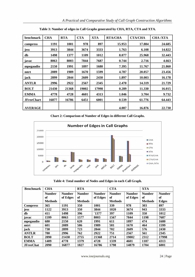
b) Number of Edges in Call Graph On comparing the number of edges in Call Graphs computed using different algorithms are shown in Table

3.The Major summary for the number of edges generated using different algorithm are as:

1. In contrast to the CHA the RTA reduces the number of edges approximately at the average of 4.087%,

provide the minimum numbers of edges reduced are about0.289% and the maximum number of edges

reduced are about 15.953%.

2. In contrast the CHA the number of edges reduced by the CTA are approximately 16.876%, provided that

the minimum number of reduced edges by CTA are 2.716% and the maximum number of edges reduced are

about 25.968%.

3. XTA when compared with the CHA comes with more precise results, it reduces the number of edges

approximately with an average of 22.730%, when the minimum number of edges reduced is about4.663%

and the maximum number of edges reduced is about 64.44%.

c) Time Elapsed

Time consumed by an algorithm depends on the how fast the worklist can be constructed and depends

on Soot framework and the nature of benchmark and the Call Graph algorithm used. The time requirement for

each algorithm with corresponding benchmark that we are able to estimate is shown in Table 5.When comparing

the time requirements for each algorithm in Soot we were able to collect following statistics:

1. The time requirements for RTA are little more than that of CHA, when computed RTA needs

approximately 1.297 more time than CHA, this may because of additional overhead of construction of extra

sets for Call Graph construction.

2. On comparing the CTA with CHA, we can observe that CTA is slower than the CHA, and more precisely

we can say that CTA 3.629 times faster than CHA.

3. When comparing the XTA with the CHA there is a significant time variation, we was able to found that XTA is on average 12.453 slower than that of CHA. This is because of its more struggles towards

preciseness and extra overhead of maintaining more sets for construction of Call Graph.

d) Memory Utilized by Call Graph algorithms Soot uses a very different memory management scheme than other bytecode readers. Depends on

memory requirements for various data structures and for how longs they need to be kept in the memory for

further use the memory requirements of benchmarks can be made. In Soot garbage collectors can remove certain

data structures for example class hierarchy information in Soot is kept in memory after Soot configuration.

Table 6 shows some of the facts about memory requirements of various Call Graph construction algorithms in

Soot.

VIII. CONCLUSION In this work we have seen how various Call Graph algorithms differ from each other in various

respects. We have analyzed that how Soot behaves with these algorithms. We can say that Soot is a Java

optimization framework which is analyzed with a lot of functions [9].the Table 7 shows the overall results

obtained from various Call Graph algorithms. According to the Table 7 we can see that compared to CHA the

RTA has better results in terms of reduction of number of edges. That average percentage number of Nodes

(reachable methods) reduced by RTA compared to CHA is 4.065%. similarly when CTA is put in front of CHA

and the number of reduced Nodes( reachable methods) is 6.551% and in compared to CHA XTA shows

significant results and reduces the number of Nodes (reachable methods) with average percentage of 20.526%.

there are cases with many benchmarks when the performance of RTA is not good as per the expectations for

example for Jack program the percentage of reduced reachable nods in just 0.959% and in Javac it is only about

1.376% but in the same time RTA has more significant performance like in programs JFreeChart and mpegaudio it reduces the number of reachable methods with a percentage of 12.584% and 8.824%. CTA as per

the Table 7 goes far behind in reducing the number of reachable methods both in individual benchmark and on

average as well for example in JFreeChart benchmark it can reduce the number of Nodes up to 13.971%. XTA

goes an extra mile in reduction process it can recdce the number of Nodes in Call Graph up to 20.526% on

average, and individually we can see for Javac program it reduced the Nodes up to 30.294 on average. The

Table 7 shows the time penalty for each of the algorithms as we move towards the higher preciseness we can see



the time requirements of algorithms also increase. RTA is 1.297 times slower than CHA and CTA is around

3.6929% slower than CHA and comparatively the CHA is 12.453 faster than XTA.

The number of edges that is present in the Call Graph computed by each algorithm brought some

interesting results to the front. When we see the number of edges reduced by RTA as compared to CHA, the

RTA reduces the number of edges with percentage about 4.087% similarly CTA reduces the number of edges a

percentage of about 16.876% and XTA comes again with good results and the number of reduction percentage is about 22.526% as compared to that of CHA. However the for this improvement the memory penalty is there.

The algorithm that reduces more number of nodes and the edges elapses more time and consumes huge amount

of memory. The details of which are present in the Table 7.

IX. FUTURE WORKS It is better to compare the static Call Graphs to their dynamic counter parts. This work can be extended

to some more Call Graph algorithms like VTA, and K-CFA [119]. Furthermore we can compare the framework

used for implementation with other available alternatives to get even more accurate and precise results. We have

the option of using Soot and ASM for construction of Call graphs and then better comparisons. In addition testing and comparing Call Graphs on different frame works will make results more general so that they can be

applied on any optimization framework. Some new dimensions in terms of metrics like line number, number of

variable, number of successors can be added for each Call Graph node and these metrics can be added to get a

new Call Graph whose every node correspond to a different kinds of metrics.

X. REFRENCES [1] Jeffrey Dean, David Grove, and Craig Chambers, Optimization of Object-oriented Programs Using Static Class Hierarchy

Analysis ECOOP 95.

[2] David Grove and Craig Chambers. A Framework for Call Graph Construction Algorithms. ACM Transactions on Programming

Languages and Systems (TOPLAS), November 2001.

[3] David Grove, Greg DeFouw, Jeffrey Dean and Craig Chambers. Call Graph Construction in Object-Oriented Languages. OOPSLA

'97: Proceedings of the 12th ACM SIGPLAN conference on Object-oriented programming, systems, Languages, and applications,

October 1997..

[4] Gail C. Murphy, David Notkin, William G. Griswold, and Erica S. lan. An Empirical Study of Static Call Graph Extractors.

Transactions on Software Engineering and Methodology (TOSEM), April 1998.

[5] Damien Sereni.Termination Analysis and Call Graph Construction for Higher- Order Functional Programs. ICFP '07: Proceedings

of the 12th ACM SIGPLAN International conference on Functional programming, October 2007.

[6] Ondrej Lhotak and David R. Cheriton. Comparing Call Graphs, Proceedings of the 7th ACM SIGPLAN-SIGSOFT workshop on

Program analysis for Software tools and engineering, June 2007.

[7] Soot: A Java Optimization Framework,March2010,http://www.sable.mcgill.ca/soot/

[8] James Gosling, Bill Joy, Guy Steele and Gilad Bracha. The Java™ Language Specification Third Edition. Addison-Wesley May

2005.

[9] Raja Vallée-Rai, Phong Co, Etienne Gagnon, Laurie Hendren, Patrick Lam and Vijay Sundaresan. Soot-a Java Bytecode

Optimization Framework. CASCON '99: Proceeding of the 1999 conference of the Centre for Advanced Studies on Collaborative

research, November 1999.

[10] F. Tip and J. Palsberg. Scalable propagation-based call graph construction algorithms. In Proceedings of the Conference on

Object-oriented Programming, Languages, Systems and Applications, pages 281–293, Oct.2000.

[11] R. Vall_ee-Rai, P. Co, E. Gagnon, L. Hendren, P. Lam, and V. Sundaresan. Soot - A Java bytecode optimization framework. In

Proc. Of CASCON,1999.

[12] D. Demange, T. Jensen, and D. Pichardie. A provably correct stackless intermediate Representation for Java bytecode. Research

Report 7021, INRIA, 2009. http://www.irisa.fr/celtique/ext/bir/rr7021.pdf.

[13] V. Benjamin Livshits, John Whaley, and Monica S. Lam. Reection analysis for Java. In Proc. of APLAS, pages 139{160. Springer,

2005.

[14] L. Hubert. A Non-Null annotation inferencer for Java bytecode. In Proc. of PASTE'08, pages 36{42. ACM, November 2008.

[15] D. R. Morrison. PATRICIA | Practical algorithm to retrieve information coded in alphanumeric. J. ACM, 15(4), 1968.

[16] Jonas Lundberg and Welf Löwe. Architecture Recovery by Semi-Automatic Component Identification. Software Technology

Group, MSI, Växjö University September 2004.

[17] Usman Ismail and David R. Cheriton. Incremental Call Graph Construction for the Eclipse IDE. School of Computer Science

University of Waterloo, 2009.

[18] Sundaresan, V., Hendren, L., Razafimahefa, C.,Vall_ee-Rai, R., Lam, P., Gagnon, E., and Godin, C.Practical virtual method call

resolution for Java. In Proceedings of the Fifteenth Annual Conference onObject-Oriented Programming Systems, Languages, and

Applications (OOPSLA'00).

[19] R. Stata and M. Abadi. A type system for Java bytecode subroutines. In Proc of POPL, 98,pages 149 60. ACM Press, 1998.

[20] Palsberg, J., and Schwartzbach, M. I. Object-orientedtype inference. In Proceedings of OOPSLA’91, ACM SIGPLAN Sixth Annual

Conference on Object-Oriented Programming Systems, Languages and Applications(Phoenix, Arizona, October 1991),

http://www.sable.mcgill.ca/soot/

http://www.irisa.fr/celtique/ext/bir/rr7021.pdf



XI. LIST OF TABLES AND GRAPHS

Table 1: Benchmark Descriptions

S.No. Benchmark Description

1. compress A high-performance application to compress or uncompress large files;

based on the Lempel-Zev method

Web reference:

www. Specbench.org.Javaclient/serverbenchmarks

2. jess A Java Expert shall systembased on NASA’s CLIP system.

Web reference: www.Specbench.org.Javaclient/serverbenchmarks

3. db Perform database functions on a memory-resident database


4. javac JDK 1.0.2 JAVA compiler Web reference:

www.Specbench.org.Javaclient/serverbenchmarks

5. mpegaudio MPEG-audio file compression application. Web reference: www.Specbench.org.Javaclient/serverbenchmarks

6. mtrt Dual-threaded version of raytrace.


7. jack A java presser generator with Lexical analyzers (now JavaCC).


8. ANTLR A language tool that provides a framework for construction of

recognizers, interpreters, compilers, and translators.

9. BLOAT It is a Java bytecode optimizer and analysis tool.

10. EMMA It is an open-source toolkit for measuring and reporting Java code.

11. JFreeChart It is an open-source java chart library, supporting a wide range of chart

types.

Table 2: number of Reachable Methods (Nodes) in CHA, RTA, CTA and XTA Call Graphs.

Benchmark CHA RTA CTA XTA RTA/CHA CTA/CHA XTA/CHA

compress 365 350 339 303 4.110 7.123 13.429

jess 1122 1104 1020 943 1.604 9.091 15.954

db 411 396 379 350 3.650 7.786 14.842

javac 1599 1577 1567 1198 1.376 2.001 25.078

mpegaudio 680 620 611 474 8.824 10.147 30.294

mtrt 601 586 581 464 2.496 3.328 22.795

jack 730 723 702 576 0.959 3.836 21.096

ANTLR 780 762 751 561 2.308 3.718 28.077

BOLT 2890 2755 2714 2312 4.671 6.090 20.000

EMMA 1409 1379 1339 1187 2.129 4.968 15.756

JFreeChart 2090 1827 1798 1704 12.584 13.971 18.469

AVERAGE 4.065 6.551 20.526

Chart 1: Comparison of Number of nodes in different Call Graphs.



Table 3: Number of edges in Call Graphs generated by CHA, RTA, CTA and XTA.

benchmark CHA RTA CTA XTA RTA/CHA CTA/CHA CHA /XTA

compress 1191 1001 978 897 15.953 17.884 24.685

jess 3913 3844 3674 3333 1.763 6.108 14.822

db 1498 1377 1109 1012 8.077 25.968 32.443

javac 8063 8003 7844 7687 0.744 2.716 4.663

mpegaudio 2150 1991 1897 1680 7.395 11.767 21.860

mtrt 2089 1989 1670 1599 4.787 20.057 23.456

jack 2899 2844 2609 2430 1.897 10.003 16.178

ANTLR 2996 2922 2567 2345 2.470 14.319 21.729

BOLT 21430 21368 19002 17998 0.289 11.330 16.015

EMMA 4778 4728 4601 4313 1.046 3.704 9.732

JFreeChart 16877 16786 6451 6001 0.539 61.776 64.443

AVERAGE 4.087 16.876 22.730

Chart 2: Comparison of Number of Edges in different Call Graphs.

Table 4: Total number of Nodes and Edges in each Call Graph.

Benchmark

CHA RTA CTA XTA

Number

of

Methods

Number

of Edges

Number

of

Methods

Number

of Edges

Number

of

Methods

Number

of Edges

Number

of

Methods

Number

of

Edges

Compress 365 1191 350 1001 339 978 303 897

jess 1122 3913 350 3844 1020 3674 943 3333

db 411 1498 396 `1377 397 1109 350 1012

javac 1599 8063 1577 8003 1567 7844 1198 7687

mpegaudio 680 2150 620 1991 611 1897 474 1680

mtrt 601 2089 586 1989 581 1670 464 1599

jack 730 2899 723 2844 702 2609 576 2430

ANTLR 780 2996 762 2922 751 2567 561 2345

BOLT 2890 21430 2755 21368 2714 19002 2312 17998

EMMA 1409 4778 1379 4728 1339 4601 1187 4313

JFreeChat 2090 16877 1827 16786 1798 14879 1704 6001



Table 5: Comparison of time elapsed by CHA, RTA, CTA, and XTA.

benchmark CHA RTA CTA XTA RTA Vs

CHA

CTA Vs

CHA

XTA Vs

CHA

compress 0.051 0.067 0.475 0.985 1.314 7.090 19.314

jess 0.122 0.14 0.259 0.847 1.148 1.850 6.943

db 0.062 0.08 0.349 2.02 1.290 4.363 32.581

javac 0.172 0.352 0.562 1.948 2.047 1.597 11.326

mpegaudio 0.081 0.097 0.317 1.302 1.198 3.268 16.074

mtrt 0.61 0.86 1.969 2.663 1.410 2.290 4.366

jack 0.091 0.121 0.624 0.955 1.330 5.157 10.495

ANTLR 0.094 0.112 0.413 1.065 1.191 3.688 11.330

BOLT 0.857 0.967 2.567 5.013 1.128 2.655 5.849

EMMA 0.192 0.211 0.832 2.528 1.099 3.943 13.167

JFreeChart 0.657 0.732 2.947 3.641 1.114 4.026 5.542

AVERAGE 1.297 3.629 12.453

Chart 3: comparison of Time Elapsed by various algorithms for construction of call Graph

Table 6: Memory used in( MB) by various Call Graph algorithms.

benchmark CHA RTA CTA XTA

compress 48 50 53 184

Jess 69 70 71 266

Db 53 54 58 192

Javac 69 70 73 296

mpegaudio 57 60 60 202

Mtrt 55 59 59 195

Jack 59 63 63 299

ANTLR 60 65 65 204

BOLT 88 91 91 452

EMMA 78 83 83 420

JFreeChart 165 172 178 552

AVERAGE 72.81818 76.09091 77.63636 296.5455



Chart 4: The amount of memory used in MB’s by various Call Graph algorithms.

Table 7: overall comparison of various algorithms

benchma

rk

RTA/C

HA

%age of

Nodes

reduced

RTA/C

HA

%age of

Edges

reduced

CHA/R

TA

average

Time

Elapsed

CTA/C

HA

%age of

Nodes

reduced

CTA/C

HA

%age of

Edges

reduced

CHA/C

TA

average

Time

Elapsed

XTA/C

HA

%age of

Nodes

reduced

XTA/C

HA

%age of

Edges

reduced

CHA/X

TA

average

Time

Elapsed

compress 4.110 15.953 1.314 7.123 17.884 7.090 13.429 24.685 19.314

jess 1.604 1.763 1.148 9.091 6.108 1.850 15.954 14.822 6.943

db 3.650 8.077 1.290 7.786 25.968 4.363 14.842 32.443 32.581

javac 1.376 0.744 2.047 2.001 2.716 1.597 25.078 4.663 11.326

mpegaud

io 8.824 7.395 1.198 10.147 11.767 3.268 30.294 21.860 16.074

mtrt 2.496 4.787 1.410 3.328 20.057 2.290 22.795 23.456 4.366

jack 0.959 1.897 1.330 3.836 10.003 5.157 21.096 16.178 10.495

ANTLR 2.308 2.470 1.191 3.718 14.319 3.688 28.077 21.729 11.330

BOLT 4.671 0.289 1.128 6.090 11.330 2.655 20.000 16.015 5.849

EMMA 2.129 1.046 1.099 4.968 3.704 3.943 15.756 9.732 13.167

JFreeCh

art 12.584 0.539 1.114 13.971 61.776 4.026 18.469 64.443 5.542

AVERA

GE 4.065 4.087 1.297 6.551 16.876 3.629 20.526 22.730 12.453

Chart 5: the overall comparison chart.

a practical and comparative study of call graph

Documents