a post-keynesian model for a
TRANSCRIPT

1
A POST-KEYNESIAN MODEL FOR ANALYZING THE
RELATIONSHIP BETWEEN DISTRIBUTION AND GROWTH
Engelbert Stockhammer* Özlem Onaran**
prepared for the
Conference on "Old and New Growth Theories: An Assessment"
October 5-7, 2001. Pisa, Italy
* Corresponding authorDept. of Economics, VWL 1Vienna University of Economics and Business AdministrationAugasse 2-61090 ViennaAustria
** Department of EconomicsIstanbul Technical UniversityITU Macka 80680 IstanbulTurkey

2
Abstract
This paper analyses of the impact of distribution on accumulation, capacity utilization andemployment, and presents a Post-Keynesian model in order to answer the question whetheraccumulation and employment are wage-led or profit-led.
The impact of distribution on growth, accumulation and employment continues to be thefocus of an ongoing debate within the discipline of macroeconomics. Does a pro-capitalredistribution of income stimulate growth, accumulation and consequently employment? Post-Keynesian macroeconomics answers this question by pointing out the dual function of wagesas a component of aggregate demand, as well as a cost item. Depending on the relativemagnitude of these dual effects, Marglin and Bhaduri (1990) distinguish between profit-ledand wage-led regimes, where the latter leads to a low rate of accumulation accompanied by ahigh profit share. This is a more general formulation of earlier neo-Kaleckian modelsanalyzing the impact of distribution on growth by Rowthorn (1982), Dutt (1984), Taylor(1985) and Blecker (1989). However, the theoretical debate in the post-Keynesian traditionstill needs to be improved in order to capture the dynamics within the system and has to besupplemented by empirical research. The lack of empirical research about the relationshipbetween distribution and growth is even more pronounced in the case of developing countries,where the pro-capital incomes policies of structural adjustment programs implemented in thelast two decades are still far from fulfilling their promises in many cases.
The model presented here is a post-Keynesian open economy model. It consists of behavioralfunctions for investments, savings, and international trade defining the goods market; theproducer's equilibrium curve, which relates capacity utilization and labor market pressures tothe distribution of income; and an employment equation. The two important contributions ofthe model presented here, compared with previous work, are employment and its effect onincome distribution. Firstly, producer's equilibrium, i.e. income distribution, is determined notonly by the pricing behavior of firms, but also by a bargaining relationship. Secondly,employment is explicitly modeled by a version of Okun's Law. These two extensionsincorporates the labor market to the analysis, allowing an interaction between distribution,accumulation, capacity utilization and employment, rather than implicitly defining labordemand as a passive outcome of the system.
The second motivation behind this study is to model the dynamic relationship betweendistribution, accumulation, capacity utilization and employment considering both lagged andcontemporaneous interactions within a systems approach, that goes beyond the limitedframework of comparative statics. Consequently we present a structural vector autoregression(SVAR) method to estimate the analytical model for selected advanced capitalist countries.This estimation, which is a novel application within the post-Keynesian literature, is,implicitly, the second aim of the paper in order to point out the driving force behindaccumulation and employment.
JEL classification: E 1, E 12, E 2, E 3
Keywords: Keynesian economics, Macroeconomics, Accumulation, Distribution, StructuralVectorautoregression

3
1. Introduction
Over the past two decades post-Keynesian macroeconomics has made significant progress.
On the one hand, reformulations of Kaleckian growth models have allowed for flexible
modelling of the goods market, while maintaining the central claim of the paramount
importance of capital accumulation and income distribution in the growth process. In
particular the Marglin-Bhaduri model (Marglin and Bhaduri 1990, Bhaduri and Marglin 1990)
has generalized earlier formulations (Rowthorn 1982, Dutt 1984, Taylor 1985) allowing for
profit-led as well as wage-led growth regimes. This shifts the actual relation between
distribution and growth to the empirical terrain such that the aggregate effect of the profit
share on accumulation depends on the relative magnitude of demand and profitability effects.
On the other hand, post-Keynesians have, theoretically as well as empirically, pointed to the
crucial role of accumulation in the determination of the level of unemployment (Rowthorn
1995, Davidson 1998, Glyn 1998, Dumenil and Levy 1999).
However, so far there is lack of empirical research. In particular those two streams of debate
are hardly combined. Moreover, the existing works fail to address the issue of simultaneity.
Bowles and Boyer (1995) as well as Gordon (1995) employ essentially single equation
approaches; Rowthorn (1995) and Glyn (1998) focus exclusively on the link between
employment and accumulation without an explicit treatment of the goods market.
The present paper is an attempt to fill this gap. The aim is to test a post-Keynesian macro
model of an open economy by means of a structural VAR model based on evidence from
major advanced capitalist countries, i.e. France, Germany, UK and USA. We wish to explore
the following features: Does accumulation play a critical role in determining capacity

4
utilization? Is employment determined by the cost of labor or by demand conditions? Are
accumulation, capacity utilization and employment wage-led or profit led?
The paper is structured as follows. Section two presents the model to be estimated and section
three reviews the previous empirical work. Section four discusses the econometric method.
Section five presents the econometric results for the tests performed. Section six discusses the
results and questions for further research, and section seven concludes.
2. The model
The model is a neo-Kaleckian model for an open private economy that allows for profit-led as
well as wage led growth regimes. The goods market part is the linearized Marglin-Bhaduri
(1990) model, which is complemented by an unemployment function that allows for
hysteresis and a distribution function that exhibits a negative effect of unemployment on real
wages, as well as a pro-cyclical mark-up pricing behavior. A somewhat simpler version of
this model is discussed analytically by Stockhammer (1999 and 2000a).
Equation (1) is the investment function (gI), proposed in Marglin and Bhaduri (1990) that
reacts positively on capacity utilization (z) and on profit share (π). a1 is known as the
accelerator effect. a2 is the positive effect of profits on accumulation. By combining these two
effects, the dual role of wages as costs and as a source of demand is integrated into the
investment function. Higher wage share will lead to higher capacity utilization, but to a lower
profit share. The net effect of an increase in the wage share on investment is thus ambiguous.
12110 −− ++= ttI
t azaag π (1)
Note that we have already imposed a certain time structure in the accumulation function:
investment is supposed to react to changes in capacity utilization and profitability only with a

5
time lag. We consider this to be the appropriate specification according to Keynesian theory.
In the short run, investment is given, because today’s investment is yesterday’s investment
decisions1. This specification introduces the time dimension to the timeless theoretical model
of Marglin and Bhaduri.
Equation (2) is a linearized form of the savings function (gS) where capacity utilization and
the profit share determine the rate of savings. b1 indicates the responsiveness of savings to
capacity utilization, i.e. the marginal propensity to consume for a given income distribution.
b2 is a positive function of the differences in savings propensity between wage incomes and
profit incomes.
ttS
t bzbg π21 += (2)
Equation (3) is a profit share function where profits depend on capacity utilization and on
unemployment (u). d1 indicates the pro-cyclicality of the mark up. d2 is the reserve army
effect, i.e. higher unemployment weakens labor’s bargaining position and therefore leads to
higher profits.
ttt udzdd 210 ++=π (3)
The profit equation deviates from earlier formulations by separating the capacity effect and
the unemployment effect. E.g. Marglin and Bhaduri (1990) and Rowthorn (1979) assumed
that unemployment and capacity move in parallel, and Bowles and Boyer (1995) take the
unemployment rate as an indicator for capacity utilization. If unemployment exhibits a high
1 Sims (1986), who was interested in money supply and demand, also chooses to have
investment contemporaneously exogenous.

6
degree of persistence, as is the case in most European countries, then it is analytically
important to distinguish between the two effects. 2
Equation (4) is an employment function that includes Okun’s law as a special case.
Accumulation and the change in capacity utilization enter separately, capacity utilization is
captured by capital productivity so that output is equal to capacity utilization times capital
stock ( zKy ≡ ). e1 is the effect of accumulation on unemployment. e2 the effect of capacity
utilization on unemployment. e3 is unemployment persistence. If e3=1 than (4) reduces to
Okun’s law.
1321 −+∆−−= tttt uezegenu (4)
Equations (3), and (4) can be combined to the analogue of Marglin and Bhaduri’s “producers’
equilibrium curve”.
Net exports (NX) are assumed to vary counter-cyclically and to be a positive function of the
profit share, which is taken as a proxy for unit labor costs and thus an indicator of
international competitiveness (Bowles and Boyer, 1995).
ttt hzhnx π21 +−= (5)
With the assumption that investment is determined by lagged variables only, i.e. that
accumulation is given in the current period we can reformulate the goods market equilibrium
condition (Equation 6) to get the following expression for capacity utilization, which we will
also refer to as effective demand function (Equation 6’).
SI gnxg =+ (6)
2 Analytically this distinction allows to identify a second equilibrium condition (equation 6) as a long run

7
( )[ ]ttt bhghb
z π2211
1 −++
= (6’)
We are now in a position to clarify the notion of profit-led vs. wage-led demand regime.
Substituting Equation (6') in (1) we get the following equilibrium growth curve as a function
of income distribution.
111
22121
11
10 −−
+−++
++= tt
It hb
bhaag
hb
aag π (7)
Depending on the sign of
+−+
11
2212 hb
bhaa the total derivative
1−t
It
d
dg
π is either positive or
negative, i.e. accumulation is either profit-led or wage-led. The sign depends on the relative
magnitudes of the direct positive effect of the profit share on accumulation (the partial
21
ag
t
It =
∂∂
−π), the positive international demand effect (
11
21
1
1
1
1
1 hb
hanx
nx
z
z
g
t
t
t
t
t
It
+=
∂∂
∂∂
∂∂
−
−
−
−
− π) and the
negative domestic consumption effect (11
21
1
1
1 hb
baz
z
g
t
t
t
It
+−=
∂∂
∂∂
−
−
− π). If the profit effect on
accumulation and net exports is high enough to offset the decline in consumption, then
accumulation is profit-led, otherwise it is wage-led.
The contemporaneous relationship between capacity utilization and profit share is also
ambiguous depending on the relative magnitudes of the domestic and international demand
effects of a higher profit share, i.e. depending on the relative magnitudes of h2 and b2. If
equilibrium (note that equilibrium here refers to a point of rest rather than to market clearing).

8
h2>b2, growth regime is exhilirationist, and is stagnationist otherwise. The lagged response of
capacity utilization to profit share also depends on both the regime of accumulation and the
relative magnitude of international and domestic demand effects3.
After experimentation, it was assumed that net exports effect capacity utilization only with a
time lag and so does the profit share in the net exports equation. Net exports very often had a
negative sign in the demand equation; similarly the profit share often had a negative sign in
the net exports equation. Thus, these effects were dropped from the contemporaneous
interactions, but will still show up in the impulse responses.
3. Review of previous empirical work
The major reference point of empirical work in this area is Bowles and Boyer (1995). Bowles
and Boyer (1995) have estimated a similar model by means of a single equation approach.
The main differences between their approach and the one taken here is in the econometric
method, but there also exist differences in the model.
Bowles and Boyer (1995) use unemployment as the indicator for capacity utilization. This is
inappropriate, especially when analyzing European unemployment, because the capacity
utilization-unemployment curve has shifted for European countries in the 1980s (Bean 1994),
which was the inspiration for capital shortage literature (Bean and Dreze 1990, Rowthorn
1995, Stockhammer, 2000b). Bowles and Boyer (1995) do extend the model to include the
state and net export.
3 See also Bhaduri and Marglin, 1990; Bowles and Boyer, 1995; Blecker, 1989 and 1999 for analyticaldiscussions about the consequences of openness on the regime of accumulation and growth, decreasing thelikelihood of a wage-led regime.

9
Bowles and Boyer (1995) estimate each of the equations separately and address the problem
of simultaneity by using lagged values for the independent variables. They do not discuss time
series properties of the variables or lag structure in any detail. But it is the problem of
simultaneity that has motivated the present study. By their approach, Bowles and Boyer
(1995) eschew the issue of simultaneity completely. Since the underlying model is an
equilibrium model, at least as far as the goods market is concerned, the appropriate way to
estimate the model is a systems approach.
In another empirical work, Gordon (1995) controls for financial variables, and cost of capital,
as well as variables that affect the relative bargaining power of labor and capital. Hein and
Krämer (1997) also adress the issue of distribution, accumulation and growth but present no
rigorous test, and are unprecise about identification issues.
4. Econometric method: Structural VAR
VAR methodology has become popular among economists since the early 1980s. Originally it
had been developed as an alternative to theory-based structural estimation. Sims (1980)
presented VAR analysis as atheoretical because it had no restrictions on the explanatory
variables and did not rely on strict exogenous-endogenous distinction. However, few
economists and econometricians hold on to such far-reaching claims. The importance of
ordering for impulse response functions has demystified the atheoretical nature of the
approach and the development of structural VAR (SVAR) has reconciled theory guided
modeling with the VAR approach.
The VAR approach is employed here for several reasons: It is a systems approach. Thus
simultaneous effects are modeled explicitly.It contains an unrestricted structural form
estimation. E.g. the Bowles and Boyer (1995) estimates are a special case of the VAR
10
estimation.Finally, it is has desirable time series properties. In particular it performs well even
in the presence of unit roots.
However, it also has shortcomings.First, the number of variables that can be integrated is
limited because VAR is an unrestricted auto-regressive distributed lag (ADL) model that
quickly runs out of degrees of freedom. Second, because it is a systems approach we do not
control for variables other than the ones in the system (this is a major difference compared to
the specifications used by Gordon 1995). Finally, the impulse response consists of short-term
reactions that cannot be readily interpreted as derivatives that we know from comparative
statics. However, they have the advantage of incorporating the joint effects of distributional
changes on accumulation and growth, which makes it possible to define whether the regime is
wage-led or profit-led.
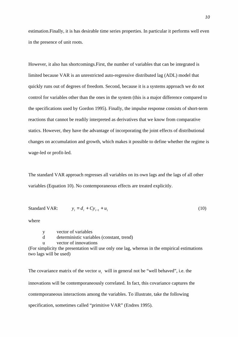
The standard VAR approach regresses all variables on its own lags and the lags of all other
variables (Equation 10). No contemporaneous effects are treated explicitly.
Standard VAR: tttt uCydy ++= −1 (10)
where
y vector of variablesd deterministic variables (constant, trend)u vector of innovations
(For simplicity the presentation will use only one lag, whereas in the empirical estimationstwo lags will be used)
The covariance matrix of the vector tu will in general not be “well behaved”, i.e. the
innovations will be contemporaneously correlated. In fact, this covariance captures the
contemporaneous interactions among the variables. To illustrate, take the following
specification, sometimes called “primitive VAR” (Endres 1995).

11
Primitive VAR : tttt AydBy ε++= −1 (11)
In this system of equations contemporaneous interactions are represented explicitly in the
matrix B. Contrary to tu in (10), tε in (11) will not be cross-correlated. Note that ABC 1−=
and tt Bu ε1−= , the latter explains the nature of cross-correlation among the errors in u.
The standard Choleski decomposition (“orthogonalization of the error covariance matrix”)
imposes a triangular structure on B that is convenient to solve, but does implicitly impose a
certain structure of contemporaneous interactions. Structural VAR makes these interactions
explicit. A necessary condition for identification is that the number of non-zero elements in
the B matrix has to be equal to or less than (n2-n)/24. However, in practice it turns out that
computational problems quickly arise if the number of the simultaneous contemporaneous
interactions increases. 5
In our case the vector y and the matrix B for the open economy case are:
=
nx
u
z
g
y π and
=
5552
444241
343332
232221
11
000
00
00
00
0000
aa
aaa
aaa
aaa
a
B , with the expected signs being
0
0
0
0
0
0
0
55
42
41
34
32
23
21
<<<>><>
a
a
a
a
a
a
a
.
and all the diagonal elements are positive by definition.
4 See Sims 1986, Bernanke 1986; Endres 1995 as an accessible textbook presentation.5 The econometrics software used, EasyReg by Bierens, frequently crashed when more than 4 variables and more
than 2 simultaneous contemporaneous interactions were being modeled.

12
The structural VAR approach proceeds in three steps. First the VAR as it is formulated in
Equation (10) is estimated. This gives coefficient estimates on lagged values and estimated
errors. In the second step these estimated errors are used to obtain estimates of the B matrix
by FIML (full information maximum likelihood) estimation. Third, impulse responses (IR),
i.e. reactions of the system to simulated exogenous shocks to each of the endogenous
variables, are calculated that combine information from both steps.
The SVAR will thus provide us with three types of information: First, the results of the VAR
itself, i.e. an unrestricted structural form in lags6. Second, the results of the contemporaneous
interactions of the error terms, which we will refer to as SVAR. Third, impulse response
functions.
The data are from the OECD Economic Outlook database. Accumulation (ACCU) is the
growth rate of the business gross capital stock, the profit share (PS) the profit share of the
business sector; unemployment (U) the national unemployment rate; net exports (NX) the
current account normalized by the capital stock of the business sector.
The measure for capacity utilization (Z) as suggested by the model is capital productivity in
the business sector. Since this is a somewhat unconventional measure of capacity utilization,
two other measures were also tried: the growth of output in the business sector (Growth) and
the output gap (GAP) as estimated by the OECD. Data Appendix presents a detailed
definition of the variables.
6 Because every variable will enter twice, with one and with two lags, multicollinearity problems will almostinevitably arise here (Bowles and Boyer (1995) specification will be a special case of the VAR).

13
The VAR consists of the five variables. A (linear) trend was added for pragmatic reasons.7
VAR analysis is appropriate for short-term analysis and the trend was statistically significant
when added. The trend captures long terms effects that are not appropriately captured in the
variables. However, the trend, though itself statistically significant, has little impact on the
parameter estimates for the other variables. It does increase some standard errors.
5. Empirical results
This section summarizes the econometric results. First, we have, as a preliminary test,
estimated the closed economy model, excluding the trade block with annual data and present
the SVAR results thereof. Second, the model is estimated for the open economy model with
semi-annual data. This will be discussed in some depth, including some tests for robustness
and impulse responses for the model with semi-annual data will be presented.
In a first step the closed economy model was estimated with yearly data for Germany, France,
UK and USA. This was done to get a simple benchmark. Results of the SVAR estimations are
summarized in Table 1.
7 Similarly Blanchard 1989 adds a trend because he cannot otherwise explain the rise in unemployment, withoutfurther theoretical justification.

14
Table 1: Structural VAR estimation for the closed private economy model (with trend)USA France Germany UK
ACCUInnovation 0.0041 *** 0.0022 *** 0.0026 *** 0.0022 ***
(4.3352) (5.8944) (5.5529) 4.8858
ZACCU 2.2712 *** 1.7972 *** 1.5422 *** 0.6024
(4.1949) (3.7791) (2.1612) (0.7855)
PS 0.0012 -0.0002 0.0001 -0.0002
(0.2002) (-0.0728) (0.0107) (-0.0140)
Innovation 0.0099 *** 0.0023 ** 0.0038 *** 0.0058
(3.1763) (2.0067) (4.8450) (0.9314)
PSZ 70.3829 *** 175.8407 * 38.6621 78.3122
(3.5460) (1.7544) (0.8332) (0.6645)
U 0.9607 *** 1.0064 0.4112 -0.0174
(3.5460) (1.1750) (1.2077) (-0.0542)
Innovation 0.3986 *** 0.5660 *** 0.4488 *** +0.5493 ***
(4.7526) (5.0267) (4.0058) (5.7073)
UGK -29.0152 -128.0210 * 49.4500 -108.7824 *
(-1.5804) (-1.6992) (1.1527) (-1.8105)
Z -37.4880 *** -0.2999 -63.9175 *** -53.0003 ***
(-4.6227) (-0.0079) (-2.4923) (-2.4157)
Innovation 0.2407 *** 0.2153 *** +0.3059 *** +0.3668 ***
(3.1763) (4.9003) (5.0632) (5.8192)
Period: 1960-98Estimations by Easyreg, Bierens (2000). t-values in parenthesis
Accumulation has a strong positive and statistically significant impact on capacity utilization.
In three of the four countries it is significant at the 1% level. The profit share has very little
impact on capacity utilization. t-values are close to zero; twice the sign is negative and twice
it is positive.
The profit share moves pro-cyclically, but at moderate significance levels (once at the 1%
once at the 10% level, but the signs are consistently positive). Unemployment has a positive
effect on the profit share, but only in the USA is the effect statistically significant.

15
Capacity utilization has a strong negative effect on unemployment that is statistically
significant at the 1% level in three countries. Accumulation has a negative effect on
unemployment, but at much lower levels of statistical significance (close to the 10% level in
three countries, insignificant “wrong sign” once).
It turns out that the results are similar to those that we get with the open economy model using
semi-annual data. The open economy model is estimated with semi-annual data for France,
UK, and USA. Germany is dropped because the combination of the structural break of
unification and the lack of availability of current account data before 1973 diminished the
number of observations.
Again a time trend was added in the VAR. Seasonal dummies were not significant and
excluded. Two lags were used in the VAR after some experimentation with lag length. Some
of the longer lags were statistically significant, but first the OLS residuals seemed well
behaved already with two lags and secondly the correlation matrices of the OLS residuals are
very similar in the 2 lags and the 4-lag case.
Due to either the complexities of the model or the software package used, the number of
simultaneous contemporaneous interactions, (such as Z depending on PS and PS depending
on Z) had to be small. This led us to drop NX from the demand function. NX therein was
insignificant and often had a negative sign, which makes no sense theoretically, but rather
indicates the negative effect of demand on net exports is captured in the demand function. For
the same reasons (low levels of significance and wrong signs) PS was not included in the NX
function. However, both the effect of NX on Z and the effect of PS on NX are visible in the
IR’s in a way consistent with theory.

16
Originally budget deficit (as a percentage of GDP) was added to test for robustness but it had
little impact on significance levels as well as IR’s of other variables and also the other
endogenous variables in the system weren't able to explain budget deficit, so it was dropped
again.
Testing for structural breaks in the SVAR was not possible. But minor experimentation with
sub-periods (especially 1960-1975 and 1980-1999) did not indicate a change in parameters.
Since capital productivity is an unconventional measure for capacity utilization, we tested the
model also with the rate of growth of real GDP and with the output gap (as calculated by the
OECD). Neither of the latter two variables is satisfying theoretically. GDP growth conflates
the theoretically important distinction between growth and capacity utilization. The output
gap has an implicit NAIRU assumption that does not go well with a Keynesian model.
However, empirically, the measure of capacity utilization makes no big difference.
Table 2 summarizes the SVAR results for France. CAPUT refers to the three different
variables that measure capacity utilization in general. ACCU has a strong impact on CAPUT
that is statistically significant at the 1% level in all three specifications. PS has no statistically
significant effect on CAPUT, but consistently has a negative sign. PS reacts positively to
CAPUT (twice at the 1% level, once at the 10% level). U has a positive effect on PS twice,
but not at conventional levels of statistical significance. ACCU has a negative strong effect on
U (twice at the 1% level). CAPUT has no statistically significant effect on U.

17
Table 2: Structural VAR estimation for the open private economy model for France
Z gap growth
ACCUInnovation 0.0006 *** 0.0006 *** 0.0005 ***
(13.7876) (12.54) (15.6399)
CAPUTACCU 2.6189 *** 849.1297 *** 6.7882 ***
(5.8736) (4.8562) (5.1234)PS -0.0001 -0.4319 -0.0002
(-0.1703) (-1.0621) (-0.0740)Innovation 0.0019 *** 0.6317 *** 0.0051 ***
(6.3275) (2.7399) (6.054)
PSCAPUT 92.1946 * 0.7049 *** 42.1536 **
(1.7354) (3.4694) (2.3544)U -0.0364 0.6766 0.5635
(-0.0596) (0.9806) (1.0594)Innovation 0.5012 *** 0.5116 *** 0.4706 ***
(12.7924 (5.9288) (13.9234)
UACCU -184.4679 *** -231.2397 ***
(-5.0278) (-5.0502)CAPUT 0.0075 0.0585 0.9956
(0.0007) (0.8628) (0.2584)Innovation 0.1478 *** 0.1746 *** 0.1745 ***
(12.2135) (8.1676) (11.3821)
NXCAPUT 50.8216 -0.1377 21.6249
(1.3316) (-1.0687) (1.2785)Innovation 0.6102 *** 0.5598 *** 0.6383 ***
(9.315) (10.0983) (8.9667)
Period: 1960-98Estimations by Easyreg, Bierens (2000). t-values in parenthesis

18
The results for the UK are summarized in Table 3. ACCU has positive impact on CAPUT
(twice at 1%, once at 10%). PS has no statistically significant effect on CAPUT. PS reacts
positively to CAPUT, but not at conventional levels of statistical significance. U has no
statistically significant effect on PS, but consistently a negative sign. CAPUT has a
statistically significant impact on U at 1% an all three specification. ACCU also has
statistically significant effect on U.
Table 3: Structural VAR estimation for the open private economy model for UK
Z growth gap
ACCUInnovation 0.0007 *** 0.0008 *** 0.0007 ***
(7.7738) (6.9954) (6.714)
CAPUTACCU 1.832 * 6.4343 *** 664.91 ***
(1.718) (2.6451) (2.9894)PS 0.0001 0.0005 0.1739
(0.0317) (0.0696) (0.3206)Innovation 0.0034 *** 0.0093 *** 0.8498 ***
(3.0369) (3.6989) (5.9171)
PSCAPUT 46.632 27.2594 0.0713
(0.4903) (1.0712) (0.2518)U -0.4798 -0.1296 -0.4575
(-0.7832) (-0.2914) (-0.7588)Innovation 0.5444 *** 0.521 *** 0.5508 ***
(7.1131) (7.8178) (7.714)
UACCU 18.4381 20.0557
(0.4687) (0.398)CAPUT -55.9417 *** -19.8928 *** -0.2094 ***
(-4.4714) (-4.4935) (-3.9271)Innovation 0.2238 *** 0.2557 *** 0.2318 ***
(7.7605) (6.4535) (7.0669)
NXCAPUT 50.0959 0.0772 -0.1711
(1.0035) (0.0055) (-1.4074)Innovation 0.7282 *** 0.6865 *** 0.7085 ***
(6.8214) 8.8794) 8.8271)
Period: 1960-98Estimations by Easyreg, Bierens (2000). t-values in parenthesis

19
The results for the USA are summarized in Table 4. ACCU has strong and statistically
significant effect on CAPUT. PS has no statistically significant effect on CAPUT. It is once
positive, once negative. PS is pro-cyclical (at 1% significance). Higher U translates into
higher PS (at 1%significance).ACCU as well as CAPUT have statistically significant negative
impact on unemployment (at 1% significance).
Table 4: Structural VAR estimation for the open private economy model for USA
z growth
ACCUInnovation 0.0012 *** 0.001 ***
(11.6274) (14.8563)
CAPUTACCU 4.7187 *** 5.6676 ***
(6.7156) (5.3642)PS -0.0003 0.0018
(-0.0872) (0.4705)Innovation 0.0061 *** 0.0073 ***
(5.3806) (6.1456)
PSCAPUT 65.2592 *** 53.7578 ***
(6.098) (7.833)U 0.8452 *** 0.7491 ***
(4.718) (4.4706)Innovation 0.3065 *** 0.3287 ***
(11.6832) (12.8218)
UACCU -87.1911 ***
(-2.3399)CAPUT -25.6033 *** -24.6797 ***
(-3.9084) (-5.7435)Innovation 0.214 *** 0.2593 ***
(12.1422) (11.4057)
NXCAPUT -9.5422 -14.3674 ***
(-1.1609) (-3.0512)Innovation 0.402 *** 0.3781 ***
(15.5987) (17.3825)
Period: 1960-98Estimations by Easyreg, Bierens (2000). t-values in parenthesis

20
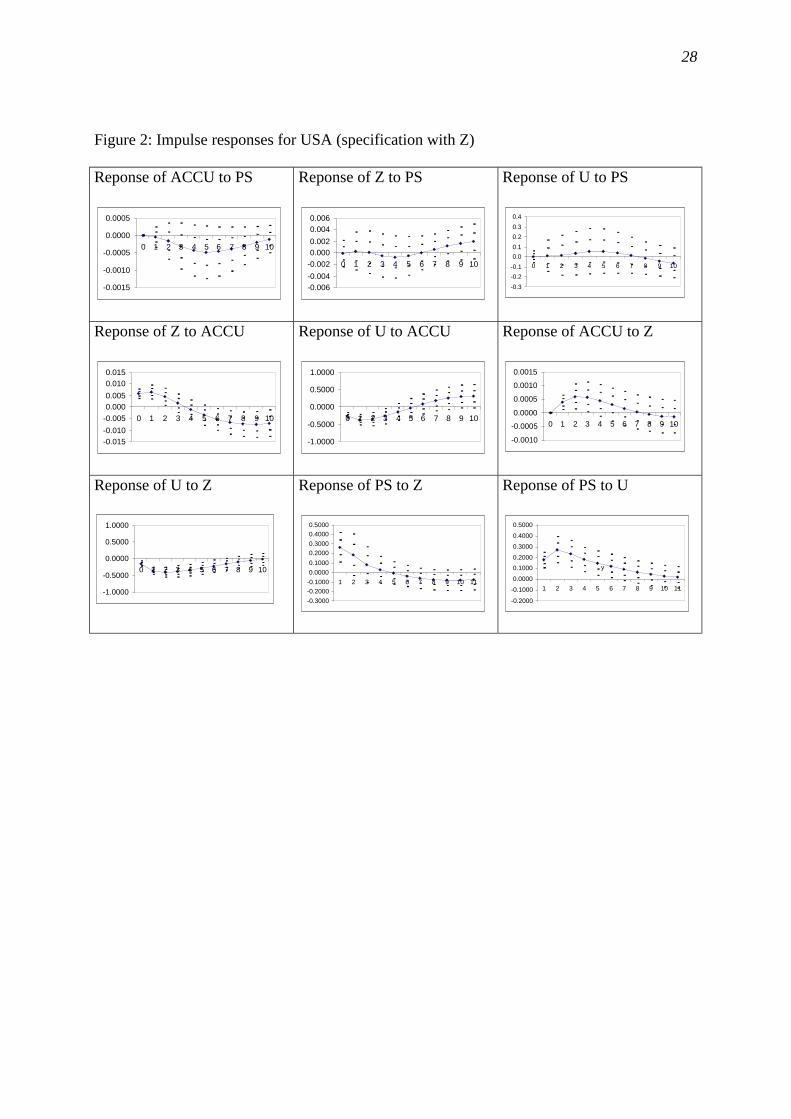
Next we turn to the impulse responses (IR). Since we have five variables, three specification
and three countries, it is impractical to give a complete presentation of the IR's. Instead, the
main results are summarized and, thereafter some IR's are presented for France and the USA
in Figure 1 and 2.
Insert Figure 1 and 2
Table 5: Summary of impulse responses
France UK USA
Accumulation
Accelerator
dACCU/dZ
yes yes yes
Accumulation regime
dACCU/dPS
wage-led (4 periods),
then profit-led
zero
(weakly wage-led)
zero
(weakly wage-led)
Demand
Effect of ACCU on
CAPUT
dZ/dACCU
yes yes yes, but short
Demand regime
dZ/dPS
stagnationist zero zero
Distribution
Reserve army effect
dPS/dU
no in SR
(yes in LR)
no in SR
(yes in LR)
yes
Procyclical profits
dPS/dZ
yes yes yes
Employment
Effect of PS on U
(dU/dPS)
yes, significant
positive
wage-led
zero zero
Effect ofdemand on U
dU/dZ and
dU/dACCU
yes yes yes
Note. Table refers to periods 0-4, i.e. 2.5 years.“zero” is used if 0 is within the 1 standard error confidence interval in all specifications.SR= short run; LR= long run

21
In compiling the table, the "short run" was, somewhat arbitrarily defined as up to the 4th
period after the shock, i.e. 2.5 years. In the later periods indirect effects will be very strong
and the system may tend to return to equilibrium. Confidence intervals are generally
disappointingly large, i.e. the estimates are not very precise. However, most patterns are
remarkably clear.
On the goods market a standard Keynesian analysis is confirmed: CAPUT has strong impact
on ACCU (unambiguously in all countries); and ACCU is an important determinant of
CAPUT (in all countries, with US only displaying a short effect). Overall, investment drives
the system, though the length of the effect varies by country and by specification.
On the labor market, too, the impulse responses correspond to a Keynesian story. CAPUT and
ACCU in all countries have a strong and long lasting effect on U in all countries. In many
cases a one-time shock to capacity utilization will have an employment effect for 5 years. The
profit share, on the other hand, has no effect (UK and USA) or even a positive effect on U in
the case of France. In other words, wage moderation does not decrease unemployment. One-
time shocks, however, do not have a permanent effect, i.e. we find no support for full
hysteresis. For practical analysis, however, this is of secondary matter.
Looking at the results for the effects of income distribution on accumulation and capacity
utilization, the results are less clear,. Neither for accumulation nor for capacity utilization are
the results significant. In most cases the one standard deviation confidence interval includes
zero. There is practically no effect of income distribution on either accumulation or capacity
utilization in the USA and the UK. For France we find some indication of a wage-led regime,
but only at modest levels of statistical significance. In other words, the model estimated failed

22
to provide us with a clear answer to whether growth is wage-led or profit-led. Potential
reasons for this failure will be discussed below.
There are, however, some interesting aspects to this failure. First, and, most surprising, is the
fact that we failed to provide evidence of the savings differential between wage income and
profit income. This should have appeared as a negative short run effect of PS on CAPUT. It
would have been unsurprising if the effect had not lasted for long. The higher PS should have
raised ACCU and NX. But in either case one had expected that these changes take more time
than the consumption effect. Moreover, the estimates for the contemporaneous effects are
positive, even if close to zero for the UK and USA. Second, the profit effect does not show up
in the IR of ACCU at all in UK and USA, and with a lag of 4 periods in France. The fact that
we get insignificant results about the causes of investment is perhaps less surprising, given the
long-standing problems in explaining investment. If the negative demand effect of high profits
were found to be significant, there would be stronger evidence to explain the mechanism
behind the irresponsiveness of investments to an increase in the profit share. This point will
be further discussed below.
A companion study (Onaran and Stockhammer 2001), which applied a similar model to the
Turkish case, did yield similar results. Together with the robustness of our results this suggest
that the results are not coincidental.
6. Open questions
There certainly are limitations of the VAR for estimating a model like the Marglin-Bhaduri
model. First, VAR methodology restricts the number of variables. Furthermore it is
impractical to add control variables, because the strength of VAR analysis is to break with a

23
clear endogenous-exogenous dichotomy, which would be resurrected by adding control
variables. Note that Gordon (1995) adds an abundance of control variables, whereas Bowles
and Boyer (1995) work with specification very similar to ours (but do use a single equation
approach).
Second, we did not test systematically for changes in the parameters, by estimating the system
for sub-periods. There is nothing in the Marglin and Bhaduri model that assumes that there is
no regime switch, and indeed Marglin and Bhaduri (1990) make the argument that the
slowdown of growth since the mid 1970s may be due to such a regime shift8. However, we
have casually estimated the system for sub periods, which gave no indication of strong
changes in parameter values or level of statistical significance. In particular, there was no
indication that the estimates of PS would improve.
Third, we have not modeled the financial sector at all. For example, if interest rates were
correlated with some of the variables employed here, which is what one would expect, the
estimates may be biased. However it is not obvious, why such a misspecification should affect
coefficients relating to income distribution more than others.
Fourth, we expected that the savings differential would become visible in the SVAR (and
early on in the IR’s), because we assumed that consumption would adjust faster than net
exports and accumulation to changes in PS. This assumption may be flawed. It is conceivable
that both consumption and, say, net exports respond with the same lags and have the same
magnitude, thus cancel out.
8 Again note that Bowles and Boyer (1995) roughly use the same time period as we do.

24
Fifth, technological change is not modeled explicitly, it will thus be hidden in some other
innovations. If the technical change is Harrod neutral, it may effect the innovation to income
distribution and also innovations to employment. This might be part of the reason, why the
profit share variable performs unsatisfactorily.
Sixth, the distribution variable, PS, may be imprecise. This is possible, especially since it is
basically the residuum of value added after wages. It thus includes financial income and
imputations for self-employment. Financial income has been rising strongly since the 1960s.
But still, the profit share is a fairly reliable indicator of the wage share and thus, assuming that
rentiers and capitalists have similar savings propensities, it should affect savings propensities.
Thus qualifications are necessary when interpreting the results with respect to the Marglin and
Bhaduri model. Overall the results hardly confirm the central role that Marglin and Bhaduri
assign income distribution, whereas they do confirm the crucial role of accumulation. Thus
our results confirm the finding by Bowles and Boyer (1995) that changes in income
distribution are unlikely to have a big effect on employment and growthay. While we get
insignificant results, Bowles and Boyer (1995) get point estimates that roughly cancel out in
the open economy case.
7. Conclusion
The aim of the paper was to test a post-Keynesian macro model of a real economy by means
of SVAR method. This method was chosen, because it is a systems approach that allows
addressing the issue of simultaneity, and simulating shocks to the system. Particular points of
interest were the role of accumulation and the role of income distribution.

25
The model employed is based on the one proposed by Marglin and Bhaduri (1990), but was
developed further by explicitly modelling the labor market and allowing for a richer
determination of income distribution. At the core of the model is the distinction between
profit-led and wage-led growth.
The results of the estimation confirmed general Keynesian assertions. Accumulation is a
crucial determinant of demand (capacity utilization) and the accelerator is key determinant of
accumulation. The level of unemployment strongly reacts to the goods market, but hardly to
changes in factor costs (here proxied by income distribution). Thus the mainstream notion that
wage moderation by itself would increase employment was clearly rejected.
However, the results fail to confirm the crucial role that Marglin and Bhaduri attribute to
functional income distribution. Neither savings differentials turned out to be statistically
significant, nor the effect of profits on accumulation. Future research needs to clarify, whether
these findings are due to the specificities of the present model or to measurement problems in
the profit share variable—or whether, indeed, income distribution has little economic effects
due to international and domestic demand effects canceling out each other.
Bibliography
Amisano, G, Giannini, C, 1997. Topics in Structural VAR Econometrics. 2nd Edition. Berlin: SpringerVerlag
Bean, Charles, 1994. European Unemployment: A Survey. JEL XXXII: 573-619Bernanke, B, 1986. Alternative Explanation of the Money Income Correlations. Carnegie Rochester
Conference Series on Public Policy 25Bhaduri, Amit, Marglin, Stephen, 1990. Unemployment and the Real Wage: The Economic Basis for
Contesting Political Ideologies. CJE, 14: 375-93Bhaskar, V, Glyn, A, 1995. Investment and profitability: the evidence from the advanced countries. In:
G Epstein and H Gintis (eds): Macroeconomic policy after the conservative era. Studies ininvestment, saving and finance. Cambridge: University Press
Bowles, S, Boyer, R, 1995. Wages, aggregate demand, and employment in an open economy: anempirical investigation. In: G Epstein and H Gintis (eds): Macroeconomic policy after theconservative era. Studies in investment, saving and finance. Cambridge: University Press

26
Charemza, W, Deadman, D, 1997. New Directions in Econometric Practice. General to SpecificModelling, Cointegration and Vector Autoregression. Aldershot: Edward Elgar
Cooley, T, LeRoy, S, 1986. Atheoretical Macroeconometrics. A critique. Journal of MonetaryEconomics 16: 283-308
Dreze, J, Bean, C, 1991. Europe's Unemployment Problem. Cambridge, Mass: MIT-PressDutt, Amitava, 1984. Stagnation, income distribution and monopoly power. CJE 8: 25-40Endres, Walter, 1995. Applied Econometric Time Series.Gordon, David, 1993. Putting Heterodox Macro to the Test: Comparing Post-Keynesian, Marxian and
Social Structuralist Macroeconometric Models for the Postwar US Economy. Working PaperNo. 43 New School for Social Research; published in Glick and Hunt (eds) 1994: Competition,Technology and Money
Gordon, David, 1995. Growth distribution, and the rules of the game: social structuralist macrofoundations for a democratic economic policy. In: G Epstein and H Gintis (eds):Macroeconomic policy after the conservative era. Studies in investment, saving and finance.Cambridge: University Press
Gordon, David, 1995. Putting the horse (back) before the cart: disentangeling the macro relationshipbetween investment and saving. In: G Epstein and H Gintis (eds): Macroeconomic policy afterthe conservative era. Studies in investment, saving and finance. Cambridge: University Press
Hein, E, Krämer, H, 1997. Income shares and capital formation: patterns of recent developments.Journcal of Income Distribution 7, 1: 5-28
Marglin, S, Bhaduri, A, 1990. Profit Squeeze and Keynesian Theory. In: S. Marglin and J. Schor (eds):The Golden Age of Capitalism. Reinterpreting the Postwar Experience. Oxford: Clarendon
Marglin, Stephen, 1984. Growth, Distribution, and Prices. Cambridge, MA: Harvard University PressOnaran, Ö, Stockhammer, E, 2001. The effect of distribution on accumulation, capacity utilization and
employment: testing the wage-led hypothesis for Turkey. Discussion Papers of the IstanbulTechnical University 01/1
Rowthorn, Bob, 1980. Capitalism, Conflict and Inflation. London: Lawrence and WishartRowthorn, R, 1981. Demand, real wages and economic growth. Thames Papers in Political Economy.
Autumn 1-39, reprinted in Studi Economici 1982, vol. 18 3-54 and also in Sawyer (ed): Post-Keynesian Economics
Rowthorn, Robert, 1995. Capital Formation and Unemployment. Oxford Review of Economic Policy11, 1: 26-39
Sims, C, Stock, J, Watson, 1990. Inference in linear time series models with some unit roots.Econometrica 58: 113-144
Sims, Christopher, 1980. Macroeconomics and reality. Econometrica 48, 1:1-48Sims, Christopher, 1986. Are Forecasting Models Usable for Policy Analysis?, Federal Reserve Bankof Minneapolis Quarterly Review, 1-16Stockhammer, Engelbert, 1999. Robinsonian and Kaleckian growth. An update on post-Keynesian
growth theories. Working paper of the Department of Economics of the University ofEconomics and Business Administration No. 67
Stockhammer, Engelbert, 2000a. Is there an equilibrium rate of unemployment in the long run?,Vienna University of Economics & B.A. Working Papers in Growth and Employment inEurope: Sustainability and Competitiveness, No. 10, February 2000
Stockhammer, Engelbert, 2000b. Explaining European Unemployment: Testing the NAIRU Theoryand a Keynesian Approach. Vienna University of Economics and Business AdministrationWorking Papers, No. 68, February 2000
Taylor, Lance, 1985. A stagnationist model of economic growth. CJE 9: 383-403

27
Figure 1: Impulse responses for France (specification with Z)
Reponse of ACCU to PS
-0.0006
-0.0004
-0.0002
0.0000
0.0002
0.0004
0.0006
0 1 2 3 4 5 6 7 8 9 10
Reponse of Z to PS
-0.0030
-0.0020
-0.0010
0.0000
0.0010
0.0020
0 1 2 3 4 5 6 7 8 9 10
Reponse of U to PS
-0.3000
-0.2000
-0.1000
0.0000
0.1000
0.2000
0.3000
0.4000
0 1 2 3 4 5 6 7 8 9 10
Reponse of Z to ACCU
-0.002
-0.001
0.000
0.001
0.002
0.003
0.004
0 1 2 3 4 5 6 7 8 9 10
Reponse of U to ACCU
-0.4000
-0.3000
-0.2000
-0.1000
0.0000
0.1000
0.2000
0 1 2 3 4 5 6 7 8 9 10
Reponse of ACCU to Z
-0.0006
-0.0004
-0.0002
0.0000
0.0002
0.0004
0.0006
0.0008
0 1 2 3 4 5 6 7 8 9 10
Reponse of U to Z
-0.4
-0.3
-0.2
-0.1
0.0
0.1
0.2
0.3
0 1 2 3 4 5 6 7 8 9 10
Reponse of PS to Z
-0.8
-0.6
-0.4
-0.2
0.0
0.2
0.4
0.6
1 2 3 4 5 6 7 8 9 10 11
Reponse of PS to U
-0.3000
-0.2000
-0.1000
0.0000
0.1000
0.2000
0.3000
0.4000
0.5000
1 2 3 4 5 6 7 8 9 10 11
28
Figure 2: Impulse responses for USA (specification with Z)
Reponse of ACCU to PS
-0.0015
-0.0010
-0.0005
0.0000
0.0005
0 1 2 3 4 5 6 7 8 9 10
Reponse of Z to PS
-0.006
-0.004
-0.002
0.000
0.002
0.004
0.006
0 1 2 3 4 5 6 7 8 9 10
Reponse of U to PS
-0.3
-0.2
-0.1
0.0
0.1
0.2
0.3
0.4
0 1 2 3 4 5 6 7 8 9 10
Reponse of Z to ACCU
-0.015
-0.010
-0.005
0.000
0.005
0.010
0.015
0 1 2 3 4 5 6 7 8 9 10
Reponse of U to ACCU
-1.0000
-0.5000
0.0000
0.5000
1.0000
0 1 2 3 4 5 6 7 8 9 10
Reponse of ACCU to Z
-0.0010
-0.0005
0.0000
0.0005
0.0010
0.0015
0 1 2 3 4 5 6 7 8 9 10
Reponse of U to Z
-1.0000
-0.5000
0.0000
0.5000
1.0000
0 1 2 3 4 5 6 7 8 9 10
Reponse of PS to Z
-0.3000
-0.2000
-0.1000
0.0000
0.1000
0.2000
0.3000
0.4000
0.5000
1 2 3 4 5 6 7 8 9 10 11
Reponse of PS to U
-0.2000
-0.1000
0.0000
0.1000
0.2000
0.3000
0.4000
0.5000
1 2 3 4 5 6 7 8 9 10 11
y

29
Data Appendix: Definition of variables
ACCU: rate of growth of business sector real gross capital stock (excludes residential capital
stock)
Z: capital productivity in the business sector
Growth: real GDP
GAP: OECD output gap
PS: profit share of the business sector
U: unemployment rate (national defintion)
NX: current account as percentage of GDP (highly correlated with current account normalized
by capital stock; correlation coefficient >.95)
Source: OECD