a post-combustion carbon capture process by amines...
TRANSCRIPT

A post-combustion carbon capture process by
amines supported on solid pellets - with estimation
of kinetic parameters
Luigi Bisone,† Sergio Bittanti,‡ Silvia Canevese,∗,† Antonio De Marco,† Simone
Garatti,‡ Maurizio Notaro,†,¶ and Valter Prandoni†
RSE S.p.A. (Ricerca sul Sistema Energetico), 20134, Milan,Italy, Dipartimento di Elettronica,
Informazione e Bioingegneria, Politecnico di Milano, Piazza Leonardo da Vinci 32, 20133,
Milan, Italy, and “Processes and catalytic materials" Laboratory, RSE S.p.A., 20134, Milan, Italy
E-mail: [email protected]
Phone: +39 02 39925696. Fax: +39 02 39925626
Abstract
A recently proposed technique for post-combustion CO2 capture in fixed-bed reactors is
based on an absorption procedure carried out by amine supported on pelleted solid substrates.
This procedure technology is less energy intensive than absorption by amines in aqueous so-
lutions. With reference to a laboratory diabatic tubular reactor, a partial differential equation
model is worked out, and, from this, an ordinary differential equation model. The description
takes into consideration the phenomenon of gas diffusion inside the porous material. In the
model there are two fundamental parameters which are uncertain: the CO2 absorption and
∗To whom correspondence should be addressed†RSE S.p.A.‡Politecnico di Milano¶RSE Laboratory
1

desorption reaction kinetic coefficients. A campaign of experiments has been performed in
the laboratory plant to collect data for estimating them. First, by means of steady-state data
we identify their ratio; subsequently, by resorting to transient data, the two parameters can be
separately estimated. The obtained model has been validated with fairly satisfactory results. A
problem in the industrial use and control of the reactor for CO2 absorption/desorption is that
constant wear during its life may cause the identified model parameters to become obsolete in
the long run. We then propose a method to automatically update their estimate.
1 Introduction
Chemical absorption by aqueous alkanolamine solvents1,2 is a viable near-term technology for
post-combustion CO2 capture from power plants flue gases.3 However, it has a number of draw-
backs, such as corrosion,4,5 foam formation6 and amine degradation due to oxidation mecha-
nisms.7 Moreover, it is highly energy intensive, especially in the sorbent regeneration stage: typical
energy penalties with monoethanolamine (MEA) or diethanolamine (DEA) processes range from
15 to 37% of the plant net power output.2,8 Therefore, many research efforts have been devoted
to conceive different kinds of technologies.9,10 Severalsolid sorbents, in particular, with or with-
out amines, have been tested.11–15Solid sorbents can achieve both higher gas absorption rate and
larger absorption capacity. Moreover, they have both lowerheat capacity and lower regeneration
temperature and thus allow an energy consumption reduction.
In this work, we focus on an innovative process16 based on chemical absorption by DEA sup-
ported on highly porous solid alumina pellets.17–19 The proposed absorbent is low cost, has high
CO2 selectivity, high absorption capacity and low specific heat,20 with, of course, good amine
stability with respect to oxidative degradation and corrosion.
The configuration of the considered CO2 capture process21 is based on a fixed-bed absorp-
tion/desorption diabatic unit operating in a TSA (Temperature Swing Absorption) mode or in a
combined TSA/PSA (Pressure Swing Absorption) mode. This unit is a finned tube heat exchanger
operating alternatively as absorber or desorber (cooled inabsorption and heated in desorption) with
2

Figure 1: RSE laboratory-scale plant and a detail of the reactor for CO2 absorption/desorption
the sorbent loaded into the free space between the fins. The fixed-bed application needs a small
pressure drop (5000Pa); hence the size of the pellets has to be wisely chosen. The best prepared
sorbents (DEA on 3 mm alumina spheres) showed a “net CO2 capture" of 50 mg CO2/g of sorbent
(5% wt) and a “useful time" of 40 minutes at 40◦C with a sorbent load of 650 g and a gas flow
rate of 300 Nl/h (gas composition: 10% CO2, 3% O2, 10% H2O in N2). The sorbent is completely
regenerated by heating the absorption unit up to 85◦C, while depressurizing it and stripping it with
a low steam flow. As compared to a conventional CO2 capture process based on a 30 wt% MEA
aqueous solution, the proposed process allows to save 35% ofthe heat required for the sorbent
regeneration, so it could be applied on a coal thermal power plant with a 3% energy saving with
respect to the MEA aqueous solution process (and with 90% efficiency).
The specific plant we deal with is the experimental equipment, shown in Figures 1 and 2 and
described in Section 2, available at the “RSE Processes and catalytic materials" laboratory located
in Piacenza (Italy). For a tutorial movie showing the preparation of the sorbent and the assem-
bling of the reactor, the reader is referred to the video available in the RSE website at the address
http://www.rse-web.it/video/Impianto-pilota-per-la-cattura-della-CO2.page.
In order to design and study a CO2 capture plant based on this technology, a reliable dynamical
model of the capture process and of the subsequent sorbent regeneration is needed. Note that the
whole process requires several batch absorption/desorption units (at least four). The model is also
3

Figure 2: RSE laboratory-scale plant flow chart
4

useful to design the automation of the coordination of theseunits.
Our model (Section 2), based on partial differential equations (PDEs), includes the description
of gas diffusion inside the porous pellets. By segmenting the reactor into a number of strips and
partitioning each pellet into a number of shells, we eventually obtain an Ordinary Differential
Equation (ODE) model (Section 3). If,e.g., one considers twenty strips and three shells for each
strip, then the final ODE model includes 160 state variables.This model suffers of the uncertainty
of the absorption and desorption reaction kinetic parameters. In Section 4, we study the problem
of estimating such parameters. The data used for this purpose have been collected in a campaign
of experiments performed in the laboratory plant. By means of steady-state data we identify first
the ratio of the two parameters; then, by analyzing the transient data, the two parameters can be
separately estimated. The obtained model has been validated with fairly satisfactory results. One
of the main problems in the industrial use and control of the reactor for CO2 absorption/desorption
is the constant wear of the reactor during its life, which maycause the identified model parameters
to become obsolete in the long run. We propose then a method toautomatically update the estimate
of the kinetic parameters.
2 Process description
The reference fixed-bed reactor of Figure 117 is constituted by a heat exchanger composed of an
inner extruded aluminium finned tube, with outer fins extending radially all along its length, and
an outer 316 stainless steel tube shell, as schematically outlined in Figure 3. The main geometric
and physical characteristics of the reactor are reported inTable 1. The sorbent is made up of
highly porous approximately spherical pellets with 36% wt.DEA contents. The sorbent fills the
space between the tube and the shell; a porous metallic disk at the bottom of the reactor supports
the pellets. A thermal fluid (diathermal oil), supplied by anexternal refrigerating and heating
circulator (see Figure 2), flows into a coil inside the tube, to avoid direct contact with the sorbent,
and it heats, or cools, by conduction the sorbent in the cavities between fins. The conductive heat
5

Table 1: Geometric and physical parameters of the considered reactor
Symbol = Value DescriptionPMDEA = 105kg/kmol DEA molecular weightA = 0.9695·10−3m2 Reactor cross section area∆ptot = 5000Pa Overall pressure drop
at nominal flow rateL = 1m Reactor lengthMs = 0.647kg Sorbent overall masspre f = p0 = 101000Pa Reference pressureRin = 0.012m Reactor inner radiusRex = 0.0225m Reactor outer radiusR0 = 1.5 ·10−3m Sorbent sphere radiusSr = [2π(Rin+Rex)+16· Metal-sorbent heat exchange·(Rex−Rin)]L = 0.385m2 surface (there are 8 fins)Tre f = T0 = 298K Reference temperatureγ = 43.3 ·106m2/m3 Active surface per unit
volume in sorbentεs = 0.4 Pellet void fractionεb = 0.4 Bulk void fractionµ = 0.15·10−4Pa·s Gas dynamic viscosityρs = 680kg/m3 Pellet mass densityϕ = 2.4145·10−8kmol/m2 Active sites per unit sorbent
surface(kmol/m2
)
wf = 287Nl/h Nominal feedgas flow rateSV= wf /Ms = 0.45Nl/(h ·g) Space velocity
exchange with the sorbent is improved by an external jacket where the thermal fluid flow rate from
the finned tube outlet can be conveyed (i.e. in an ideally series configuration).
The temperature of the fixed-bed sorbent is measured by threetype K thermocouples placed
respectively at the beginning (point A), at the end (point B)and in the middle (point C) of the
sorbent bed. The inlet and the outlet reactor gas composition are measured by continuous analyzers
specifically designed for CO2 and recorded by a data logger with 1 Hz sample rate. A vacuum
pump depressurizes the reactor during the regeneration carried out as a combination of TSA and
PSA modes.
The reactor is schematically represented in Figure 3; the bulk gas flows along the axial coordi-
6

Figure 3: Left: schematic structure of the absorption/desorption reactor; right: reference structurefor the reactor model
natez. The pellets are represented as spheres of radiusR0. Absorption and desorption occur inside
each sphere, as depicted in Figure 4. The overall reaction onthe sorbent surface is
2R2NH︸ ︷︷ ︸DEA
+CO2
abs
⇄
des
R2NH+2 +R2NCO−2︸ ︷︷ ︸
DEA∗
. (1)
In the absorption phase, the feedgas mixture reaches the sphere outer surface crossing its limit
layer (step 1); then, it flows inside the sphere, into its pores (step 2); once it reaches the surface
with the anchored DEA, the exothermal CO2 absorption reaction occurs (step 3); in the desorption
phase, the reverse reaction occurs, CO2 is released (step 4) and leaves the pellet (step 5) to reach
the bulk flow.
In order to describe the reactor dynamic behaviour, it is necessary to take into account not
7

Figure 4: The main steps of the absorption/desorption process inside pellets
only mass and energy exchanges along the gas bulk flow, but also the ones which are due to
the absorption/desorption steps and those between gas in the spheres and gas in the bulk region;
besides, additional thermal fluxes have to be considered dueto the fact that the reactor is a finned
tube and that there is the heating/cooling bath to control the sorbent temperature. All these issues
are now considered one by one and then described in mathematical form:
• fluid-dynamic and chemical phenomena:
– mass transport along the reactor bulk, in the gas motion direction (i.e. along coordinate
z): this is essentially due to convection and diffusion alongthe reactor axial coordinate;
diffusion is neglected in the radial directionr;
– mass exchange between the bulk gas and gas inside the pellets, which is due both to
convection and to diffusion (in the absorption phase,e.g., CO2 diffuses from the bulk
into the pellets, while N2 diffuses towards the bulk);
– gas motion inside each average spherical pellet, due to diffusion and to convection
(along coordinateR);
– momentum transport and friction losses along the bulk gas flow, in the reactor axial
8

direction;
– momentum transport and friction losses related to gas flow inside the spherical pellets
(along the radial directionR in each sphere);
– CO2 absorption/desorption mechanisms on the sorbent active surface, inside each sphere;
these are strictly related to the reaction chemical kinetics;
• thermal phenomena:
– heat generation/consumption due to the CO2 absorption/desorption reaction inside the
pellets, on their porous surface where the amine is anchored;
– diffusive heat flux, both in the gas and in the solid sorbent material, along the reactor
radial directionr;
– diffusive heat flux in the sorbent material along the reactorlongitudinal directionz;
– thermal convective exchange between pellets and bulk gas;
– thermal convective exchange between pellets and metal (i.e. the inner and outer pipes
surface and the fins surface);
– convective energy transport in the bulk gas along the feedgas mixture main motion
directionz.
To capture all these phenomena, we have developed a two-foldPartial Differential Equation
(PDE) model, relating the description of the overall reactor dynamics to a microscopic description
of reaction dynamics on the porous pellets inner surface. More precisely, two-dimensional (2-D)
conservation equations, with partial derivatives with respect to the reactor longitudinal coordinate
zand the reactor radial coordinater, are adopted for the reactor temperature dynamics,22 as a result
of the interaction between the feedgas flow and the absorption/desorption reaction in the porous
pellets; this description is complemented with one-dimensional (1-D) conservation equations, with
partial derivatives with respect to the pellet radial coordinateR, for temperature inside pellets. The
dynamics of the chemical variables (molar concentrations and active sites, see Section 2.2.2 and
9

Santacesaria et al.23) and of fluid-dynamic variables (molar flow rates and pressures) are described
by 1-D conservation equations (alongz) for the bulk flow, interacting with 1-D conservation equa-
tions (alongR) inside the pellet particles.
A preliminary congress presentation on our research activity can be found in Bisone et al..24
Various models are available in the literature; in some of them, e.g. Santacesaria et al.23),
the bulk flow dynamics are integrated with analgebraicdescription of chemical kinetics inside
the pellets, for which different absorption mechanisms (compare Foo and Hameed25) have been
successfully proposed. In Ruthven’s books Ruthven,26 Ruthven et al.,27 chemical kinetics as well
are treated in adynamicway. In the model proposed herewith, chemical kineticsdynamicsare
described, by making particular reference to the pellet porous surface and taking care of diffusion
inside the porous pellets as well; this leads to writing all mass conservation equations inside the
pellet spherical volume as distributed-parameter equations.
To properly introduce the equations, we are well advised to make a reference to Table 2, where
the adopted list of symbols is displayed. For convenience ofnotation, for some variables (such
as molar densities and molar concentrations) the same symbol will be employed inside the bulk
gas and inside the pellet gas, since the reference volume will be specified when introducing each
equation.
Table 2: PDE model nomenclature
Symbol Description Unit
A reactor cross section area m2
Ag cross section area in the gas phase m2
CCO2 CO2 molar concentration (in the bulk gas kmol/m3
or in the pellet gas)
Cre f reference molar concentration value kmol/m3
cpg gas molar specific heat at constant pressure kJ/kmol
cvg gas molar specific heat at constant volume kJ/kmol
Table 2: continues in the next page
10

Table 2: continues from previous page
Symbol Description Unit
cs solid phase mass specific heat kJ/kg
D0 pellet diameter m
DCO2 CO2 axial mass diffusion coefficient m2/s
DCO2,R CO2 mass radial diffusion coefficient m2/s
(along the pellet radius)
Hs reaction heat J/kmol
kabs absorption reaction kinetic parameter m/s
kdes desorption reaction kinetic parameter m/s
kf r friction coefficient in the bulk volume kmol/(m3s)
L reactor length m
n′′′ number of pellets per unit volume of the reactor m−3
PM average molar weight of the bulk gas mixture kg/kmol
p pressure Pa
pre f reference pressure value Pa
R pellet radial coordinate m
R0 pellet radius m
Rg universal gas constant J/(K ·mol)
r reactor radius coordinate m
Tg temperature in the bulk volume gas phase K
Tre f reference temperature value K
Ts temperature in the bulk volume solid phase K
ug bulk gas velocity m/s
uR radial gas velocity inside the pellets m/s
w gas axial molar flow rate along the bulk kmol/s
Table 2: continues in the next page
11

Table 2: continues from previous page
Symbol Description Unit
w′conv,s gas convective molar flow rate per unit length kmol/(sm)
from the bulk towards the pellets outer surface
w′CO2,dCO2 diffusive molar flow rate per unit length kmol/(sm)
from the bulk towards the pellets outer surface
w′′′sup CO2 local molar flow rate, per unit volume, kmol/(m3s)
from the gas phase inside the pellet towards
the pellet surface
xCO2 CO2 molar fraction (in the bulk gas or in the pellet gas)−
xCO2,s CO2 molar fraction on the pellets outer surface −
z reactor axial coordinate m
γ active surface of a pellet per unit pellet volume m2/m3
γsg heat transfer coefficient between the pellet W/(m2K)
external surface and the gas in the bulk
λs,r thermal conductivity for the thermal radial diffusive W/(m2K)
flux in the solid phase
λs,z thermal conductivity for the thermal axial diffusive W/(m2K)
flux in the solid phase
εg reactor void fraction −
εp pellet void fraction −
θ activated site area fraction −
ρ gas molar density (in the bulk volume or inside kmol/m3
the pellet volume)
ρs solid phase mass density kg/m3
ϕ thekmolof DEA sites which can be occupied kmol/m2
Table 2: continues in the next page
12

Table 2: continues from previous page
Symbol Description Unit
by CO2 in 1 m2 of active surface
Table 2: end
2.1 Bulk equations
2.1.1 1-D Mass Conservation Equations
In the reactor bulk volume, two main mass conservation equations are considered: the overall
mass conservation equation and CO2 mass conservation equation. Both of them are written in
molar form, for convenience.
The overall mass conservation equation,i.e. for all gaseous species, can be written as
∂ ρAg
∂ t+
∂ w∂z
=−w′conv,s, (2)
whereAg is the effective cross section area in the gas phase, namelyAg = Aεg; in turn, εg is the
reactor void fraction,i.e. εg = (reactor total volume - total solid volume in the reactor)/reactor total
volume;w= ρAgug is the gas axial molar flow rate andρ = p/(RgTg) is the bulk gas molar density.
The two terms on the left-hand side are the accumulation and the transport terms along the axial
directionz (the bulk flow direction). The term on the right-hand side accounts for the convective
mass exchange, in terms of molar flow rate per unit length, between the bulk and the pellets outer
surface.
The mass conservation equation for CO2 only reads as
∂CCO2Ag
∂ t+
∂ wxCO2
∂z−
∂∂z
(AgDCO2
∂CCO2
∂z
)=−w′conv,sxCO2,s− w′CO2,d, (3)
whereCCO2 andxCO2 are CO2 molar concentration and molar fraction respectively, in the bulk gas;
of course,CCO2 = ρxCO2. w′conv,s is the gas convective molar flow rate, per unit length, towards
13

the pellets outer surface, while ˜w′CO2,dis CO2 diffusive molar flow rate, per unit length, towards
the pellets outer surface (see Section 2.2.1). The three terms on the left-hand side are the usual
CO2 accumulation, transport and diffusion term, respectively, along the axial directionz, while the
two terms on the right-hand side account for CO2 convective and diffusion motion, in terms of
molar flow rate per unit length, between the bulk and the pellets outer surface. As for the diffusion
coefficientDCO2, we have assumed the classical binary diffusion of CO2 in N2.
2.1.2 Linear Momentum Conservation Equation
Momentum conservation equation in the bulk volume can be written as
∂ w∂ t
+∂Agρu2
∂z+Ag
∂ p∂z
+kf rwρ= 0, (4)
where, from left to right, the usual accumulation, transport, pressure and friction terms appear. The
friction coefficientkf r can be expressed as the combination of a “laminar” and a “turbulent” term
(see the Ergun correlation in Bird et al.28 and in Froment and Bischoff29)
kf r = kl +ks|w|, (5)
with
kl = 150(1− εg)
2
ε2g
µD2
0
ks= 1.751− εg
ε2g
PM
D20A
where, we remind,εg is the bulk void fraction andD0 the pellet diameter, whilePM is the average
molar weight of the gas mixture.
2.1.3 Energy Conservation Equations
In the bulk volume, again, two main energy conservation equations are taken into account, for the
gas phase and for the solid phase respectively.
14

Energy conservation for the gas phase can be written as
∂2πrρ cvgTg
∂ t+ w′′g2πrcpg
∂Tg
∂z= 2πrn′′′4πR2
0γsg(Ts−Tg) , (6)
whereTg is the gas phase temperature,cvg andcpg the gas molar specific heat at constant volume
and at constant pressure respectively, ˜w′′g = w/Ag andγsg is the heat transfer coefficient between
the pellet external surface and the gas in the bulk. The termson left-hand side describe energy
accumulation and convective transport along the axial direction z, while the term on the right-
hand side accounts for heat exchange between the gas phase and the solid phase. Indeed,Ts is
the solid phase temperature, whilen′′′ is the number of pellets per unit volume of the reactor (we
remind that the ideal average pellet is assumed as a sphere ofradiusR0). Diffusion along the
reactor axial directionz has not been included, since it is negligible with respect tothe convective
transport term. Diffusion along the reactor radial direction r has not been included explicitly in
this equation, because it is accounted for by the thermal conductivity and heat exchange coefficient
in the solid phase energy conservation equation (see Froment and Bischoff29 and parameterλs in
(7)).
Energy conservation equation of the solid phase (2-D) can bewritten as
∂2πrρscsTs
∂ t+
∂∂ r
(2πrλs,r
∂Ts
∂ r
)+
∂∂z
(2πrλs,z
∂Ts
∂z
)= Es2πr−2πrn′′′4πR2
0γsg(Ts−Tg) , (7)
whereTs is the solid phase temperature, whileρs andcs the solid phase mass density and spe-
cific heat respectively. The terms on left-hand side describe energy accumulation (in the solid
phase), diffusion along the reactor radial directionr and along the reactor axial directionz, while
the terms on the right-hand side account for the absorption/desorption reaction energy genera-
tion/consumption and, as in the previous equation, for heatexchange between the solid phase and
the gas phase. The heat transfer coefficientγsg, between the pellet surface and the gas phase, has
been evaluated here by a Colburn formula30 where the Nusselt number of the particles is related
to the Reynolds number of the particles and the Prandtl number of the fluid. The radial diffusive
15

thermal flux has been considered for the solid phase only, as already remarked; obviously, the cor-
relation (Froment and Bischoff,29 Section 11.7, and Balakrishnan and Pei30) adopted for thermal
conductivityλs,r in the radial direction accounts for the presence not only ofthe solid phase but
also of the gas phase. The axial diffusive thermal flux, instead, regards the solid phase only, with
its thermal conductivityλs,z, which has been computed in a simple way as the product of alumina
conductivity and the factor(1− εg).
Es2πr is the power flux (W/m2) released/absorbed by the CO2 absorption/desorption reaction
on the pellet porous inner surface,i.e. the product of the reaction heatHs and of the reacting moles:
Es=∫ R0
04πR2γHsn
′′′[kabs(1−θ)CCO2−kdesθCre f
]dR, (8)
whereR0 is the pellet radius,γ the active surface of a pellet per unit pellet volume, andθ the inner
area fraction occupied by absorbed CO2 molecules;kabs andkdes are absorption and desorption
coefficients describing the reaction kinetics (see Section2.2.2).
2.2 Conservation equations in the pellet volume
2.2.1 1-D Mass Conservation Equations
In the pellet volume, two main mass conservation equations are considered: the overall mass
conservation equation and CO2 mass conservation equation, as in the bulk volume. Again, both of
them are written in molar form, for convenience.
Mass conservation equation for all species in the gas phase inside pellets can be written as
∂∂ t
(4πR2εpρ
)+
∂∂R
(4πR2εpρuR
)=−4πR2w′′′sup, (9)
whereεp is the pellet void fraction,uR the gas velocity inside pellets and ˜w′′′sup the molar flow
rate, per unit volume, between the gas phase inside the pellet and the pellet surface (due to CO2
absorption/desorption, see Section 2.2.2). The terms on the left-hand side account for accumulation
16

and for radial transport respectively. Notice thatρ , namely gas molar density inside pellets, is
computed at temperatureTs.
Mass conservation equation for CO2 inside the pellets reads as
∂∂ t
(4πR2εpCCO2
)+
∂∂R
(4πR2εpρuRxCO2
)−
∂∂R
(4πR2
DCO2,Rεp∂CCO2
∂R
)=−4πR2w′′′sup, (10)
with the accumulation term, the radial transport term and the radial diffusion term on the left-hand
side; notice thatCCO2 ≡ CCO2(R,z, t) andxCO2 ≡ xCO2(R,z, t) are CO2 molar concentration and
molar fraction, respectively, in the gas phase inside pellets.
As for parameterDCO2,R, i.e. CO2 mass radial diffusion coefficient, describing diffusion inside
the porous pellet, a simple correlation based on the “dusty-gas” model has been adopted,31 taking
into account inner porosity (the ratio of the pores volume and the particle volume), inner surface
per unit mass, Knudsen diffusivity (which is related to tortuosity for instance) and binary diffusion.
Subtracting (10) from (9) side by side and assuming that∂CCO2 = ρ∂xCO2 (based on the further
assumption that pressure and temperature are uniform in thegas phase inside the pellet) yields
∂∂ t
[4πR2εpρ (1−xCO2)
]+
∂∂R
[4πR2εpρuR(1−xCO2)
]+
∂∂R
(4πR2
DCO2,Rεpρ∂xCO2
∂R
)= 0.
(11)
Thus, integrating both sides, with respect toR, between 0 andR, one obtains
∂∂ t
∫ R
0
[4πξ 2εpρ (1−xCO2)
]dξ +4πR2εpρ
[uR(1−xCO2)+DCO2,R
∂xCO2
∂R
]= 0. (12)
Therefore,
uR =−1
1−xCO2
[DCO2,R
∂xCO2
∂R+
14πR2εpρ
∂∂ t
∫ R
0
[4πξ 2εpρ (1−xCO2)
]dξ
]. (13)
17

Now, replacing this expression in (10) gives
∂∂ t
(4πR2εpρxCO2
)−
∂∂R
(4πR2εpρ
DCO2,R
1−xCO2
∂xCO2
∂R
)+
−∂
∂R
(xCO2
1−xCO2
∂∂ t
∫ R
0
[4πξ 2εpρ (1−xCO2)
]dξ
)=−4πR2w′′′sup. (14)
The related boundary condition accounts for CO2 mass transfer between the bulk and the pellet
gas, due to CO2 convective and diffusive flux on the pellet surface,i.e. for R= R0. Remind that
xCO2,s (see (3), in Section 2.1.1) is the CO2 molar fraction on the pellet surface, namelyxCO2|R=R0.
The CO2 convective molar flow rate on the pellet surface can be written as
wconv,sxCO2,s= 4πR20εp(ρuRxCO2) |R=R0 =−4πR2
0εpDCO2,Rρ(
xCO2
1−xCO2
∂xCO2
∂R
)∣∣∣∣∣R=R0
=
=−4πR20εpDCO2,Rρ
xCO2,s
1−xCO2,s
(∂xCO2
∂R
)∣∣∣∣∣R=R0
(15)
and CO2 diffusive molar flow rate as
wCO2,d = 4πR20εpDCO2,Rρ
(∂xCO2
∂R
)∣∣∣∣∣R0
; (16)
therefore, the boundary condition reads
4πR20hCO2
(xCO2,bulk−xCO2,s
)= 4πR2
0DCO2,Rρ1
1−xCO2,s
(∂xCO2
∂R
)∣∣∣∣∣R=R0
, (17)
wherehCO2 is a suitable CO2 mass (molar) transfer coefficient.
Of course, CO2 convective and diffusive molar flow rates per unit length on the right-hand
side of (3), namely ˜w′conv,sxCO2,s andw′CO2,d, are related to the just computed CO2 convective and
diffusive molar flow rates on the pellet surface by the pelletdensity per unit lengthNp/L, where
18
Np is the number of pellets in the reactor andL is the reactor length:
w′conv,sxCO2,s= wconv,sxCO2,sNp
L(18)
w′CO2,d = wCO2,dNp
L(19)
Finally, we remark that, in casexCO2→ 1, i.e. in case there is CO2 only in the gas mixture (as it
happens in the desorbing stage of the overall process), thenthere is no CO2 diffusion, so equation
(10) disappears from the model, while equation (9) still holds.
2.2.2 Chemical kinetics
The Langmuir theory29 (compare also Serna-Guerrero and Sayari,32 for a discussion of different
approaches to kinetic dynamics) can be employed to describeCO2 absorption and desorption into
the sorbent. Letθ be the area fraction occupied by CO2 molecules tied to the DEA on the porous
medium surface,CCO2 CO2 molar concentration, in the gas phase, in the porous medium,Ts the
sorbent temperature (assumed as uniform alongR), ϕ thekmolof DEA sites which can be occupied
by CO2 in 1 m2 of active surface. Then, reaction kinetics can be describedby the conservation
equation
ϕ∂θ(z, r,R, t)
∂ t= kabs(Ts(z, r, t)) ·CCO2(z, r,R, t) · (1−θ(z, r,R, t))+
−kdes(Ts(z, r, t))Cre fθ(z, r,R, t). (20)
where the reference molar concentration isCre f = pre f/(RgTre f ) (the reference pressure and tem-
perature, here, are assumed as the standard conditions values, i.e. pre f = 101000Pa andTre f =
298K). kabs and kdes are, respectively, the absorption and desorption kinetic parameters in the
reaction between CO2 and DEA sites.
The CO2 molar flow rate per unit volume ˜w′′′sup in (9) and (10) is, of course, directly related to
19

the reaction kinetic equation (20):
w′′′sup= γ[kabs(Ts(z, r, t))CCO2(z, r,R, t)(1−θ(z, r,R, t))−kdes(Ts(z, r, t))Cre fθ(z, r,R, t)
], (21)
whereγ is defined as the ratio of the total surface, inside pellets, where there are active sites and
the volume of the pellets.
kabsandkdesare the main uncertain parameters in the model. The problem of their identification
will be addressed in Section 4.
2.2.3 Momentum Conservation Equation Inside the Pellet
In principle, the model would require a momentum conservation equation in the pellet as well:
∂∂ t
(4πR2ρuR
)+
∂∂R
(4πR2ρu2
R
)+4πR2 ∂ p
∂R−4πR2kf r,pρuR = 0, (22)
where, from left to right, the usual accumulation, transport (along the radial coordinateR inside
the pellets), pressure and friction terms appear.
However, for simplicity, here we have assumed that the pressure is uniform inside the pellet
and equal to the bulk pressure. Further inquiries on this approximation are currently underway.
3 Finite-dimensional model
By means of a finite-volume approach, we have derived an Ordinary Differential Equation (ODE)
model (Table 3) from the PDE model of the previous section.
In few words, the reactor lengthL is divided intoNc strips (see Figure 3), in each of which the
bulk gas behaviour is described by ordinary differential mass, energy and momentum conservation
equations, obtained by integrating the PDEs just describedalong the spatial coordinatez first,
along the bulk gas flow direction, and then along the radial coordinater. The process variables in
the generick-th strip, ∆zk long, betweenzk andzk+1, are defined by their average value alongz
20

betweenzk andzk+1. For convective fluxes of energy and mass an upstream formulation has been
adopted. Momentum conservation equations have been integrated in staggered cells with respect
to the mass and energy conservation equations, so they are employed to define the molar flow rates
at the junctions between adjacent strips. For simplicity, all strips are assumed as identical width:
∆zk = ∆z= L/Nc, ∀k= 0, . . . ,Nc−1.
Similarly, an average equivalent spherical pellet, of radiusR0, is divided intoNr spherical shell
volumes and ordinary differential mass conservation equations and chemical kinetics equations are
considered in eachi-th shell, i = 0, . . . ,Nr−1. Here, all shells are assumed as the same volume
Vg = 4πR03/(3Nr). In the conservation equations for the bulk region, the “effect" of a single pellet
is multiplied by the average number of pellets in a strip, i.e. Np∆z/L, with Np the total number of
pellets in the reactor.
Integration along the reactor radial coordinater allows to write energy conservation equations
in the sorbent with reference to a sorbent average temperatureTk in each stripk.
One can verify that the momentum and mass accumulation termsin the bulk gas volume,
namely the terms related to pressure and flow rate wave propagation, have very small time-scale
dynamics, so they give rise to stiff equations; therefore, the quasi-steady state assumption has been
made. The same assumption is valid for the momentum conservation equations in the porous pellet
volume; moreover, radial convective flow in the pellets is very small, indeed it is zero at steady
state, so pressure inside the pellet has been assumed to coincide with the fluid pressure in the bulk
region adjacent to the pellet (in other words, the friction term in the radial momentum conservation
equations has been neglected).
Hydrodynamic boundary conditions for the reactor inlet and/or outlet have been set as (see the
two black boxes at the top and bottom of the reactor, in Figure3)
σAwb(0, t) = αA(pA(t)− p0(t))+σAwA(t) (23)
σBwb(Nc, t) = αB(p1(t)− pB(t))−σBwB(t), (24)
21

wherewb(0, t) andwb(Nc, t) are the reactor inlet and outlet molar flow rates,p0 andp1 are the inlet
and outlet pressures,σA, σB, αA andαB are suitable coefficients. For instance,
• for {σA = 1,αA = 0,σB = 0,αB = 1}, the reactor outlet pressure is set asp1(t) = pB(t)
and the injected inlet flow rate iswb(0, t) = wA(t), wherepB(t) andwA(t) are an assigned
pressure and flow rate, respectively;
• for {σA = 1,αA = 0,wA = 0,σB = 0,αB = 1}, one hasp1(t) = pB(t) andwb(0, t) = 0, as in
the heating phase while CO2 exits through terminal B.
Boundary conditions for bulk energy conservation equations are expressed by means of tem-
peraturesTA and TB and of CO2 molar fractionsxA and xB. For instance, ifwb(0, t)≥ 0, at
point A there are an entering CO2 molar flow ratewb(0, t)xA(t) and entering convective power
wb(0, t)Cp(TA)TA(t); if wb(0, t)< 0, instead,xA andTA, and therefore the exiting molar flow rate
and the exiting convective power are computed by the model. Similar considerations can be drawn
at point B for flow ratewb(Nc, t): if wb(Nc, t) < 0, for instance, there are molar flow rate and
convective power flow entering B, and their values are determined byxB andTB.
The obtained overall model includesN = 2Nc(Nr +1) state equations (with our choiceNc = 20
andNr = 3, 160 state equations). It also includes a number of algebraic equations. The model
has been implemented by a stand-alone C codex, which can be easily connected industrial plant
simulators; besides, it is useful for identification purposes, as described in the subsequent sections.
4 Kinetic parameters identification via bench experiments
The ODE version of the kinetics equation (20) is
ϕθk,i(t) = kabs(Ts,k(t)
)·(1−θk,i(t)
)·Ck,i(t)−kdes
(Ts,k(t)
)·Cre f ·θk,i(t), (25)
wherei is the shell index andk the strip index. The main uncertain parameters are the absorption
and desorption kinetic coefficientskabs and kdes, which strongly depend on temperature in the
22

Table 3: ODE model synopsis (CE = Conservation Equation)
Chemical kineticsActive site CE, for i= 1, . . . ,Nr , k= 0, . . . ,Nc−1:- CO2 absorption and desorption into the pellet (see (25)).
Hydrodynamic equationsGlobal mass CE in the pellet, for i= 1, . . . ,Nr , k= 0, . . . ,Nc−1 :- quasi-steady state conditions;- no convective flow rate at the sphere centre;- bulk-sorbent boundary flow rate due to absorption from all shells;Global mass CE along the bulk flow, for k= 0, . . . ,Nc−1 :- no accumulation (quasi-stationary assumption forp andT).Momentum CE in the bulk region, for k= 0, . . . ,Nc :- quasi-steady state conditions;- laminar friction only.
Mass conservation equationsCO2 mass CE in the pellet volume, for i= 0, . . . ,Nr −1, k= 0, . . . ,Nc−1 :- CO2 accumulation;- CO2 absorption/desorption;- CO2 radial diffusion, to/from the adjacent shells;- CO2 radial convection, to/from the adjacent shells.CO2 mass CE in the bulk volume, for k= 0, . . . ,Nc−1 :- CO2 accumulation;- CO2 convective and diffusive mass exchange with the pellet surface;- CO2 bulk axial diffusion, to/from the adjacent strips;- CO2 bulk axial convection, to/from the adjacent strips.
Energy conservation equationsEnergy CE in the sorbent volume, for k= 0, . . . ,Nc−1 :- energy accumulation;- conduction in the reactor axial direction, to/from the adjacent strips;- absorption/desorption reaction heat;- heat exchange between the pellets and the bulk gas;- heat exchange between the pellets and the exchanger metal surface.Energy CEs in the bulk volume, for k= 0, . . . ,Nc−1 :- accumulation is neglected in the bulk gas;- heat exchange between the pellets and the bulk gas;- energy axial transport to/from the adjacent strips, by bulk flow rate;- energy axial conduction, to/from the adjacent strips.
porous medium.
The identification procedure is based on data collected in twelvead hocdynamic experiments
23

carried out on the test rig. Each experiment started from completely regenerated sorbent. Ab-
sorption was carried out by feeding the reactor with N2, steam (10% molar fraction) and CO2
mixtures with fixed CO2 concentrations, setting the inlet gas flow rates by means of the mass-flow
controllers (wf = 219 Nl/h was the total feedgas flow rate), and keeping the reactor temperature
constant and uniform by using the external circulator. Three different inlet mixtures (with CO2
molar fraction equal to 0.05, 0.10 and 0.25) and four temperatures (25◦C, 40 ◦C, 60 ◦C and 85
◦C) have been considered: this way, we have collected twelve sequences of data, each one cor-
responding to a pair (molar fraction, temperature), with sample rate 1 Hz. In each test, the CO2
molar fraction at the reactor outletxCO2out was measured, up to the final steady state of complete
sorbent saturation (θ = 1 in (25)). As for the temperatureTs,k, we have used the values provided
by our model; notice in passing that, in the reactor sectionswhere the three thermocouples are
placed (beginning, middle, end), the temperature suppliedby the model is in fair agreement with
the measured temperature.
The adopted estimation procedure can be summarized as follows:
1. identification of the ratioη := kabs/kdesvia steady-state data.
By means of the measurements ofxCO2out, it has been possible to evaluate the steady-state
value of the amount of adsorbed CO2 in each test, namelyΓ (kmol). The corresponding
twelve points are depicted in Figure 5. The obtained values for Γ have been employed to
evaluate (pointwise) the twelve values of the ratioη := kabs/kdes. They have also allowed
the evaluation of the standard enthalpy variation of reaction (1), which, in turn, has allowed
the determination ofη as a function of the temperature.
2. Identification of kabs and kdesvia transient data.
The values ofη identified as indicated in the previous point, together withtransientdata
gathered from the experiments have been used to identifykabs andkdesseparately (as func-
tions of the temperature). In this phase, we have used three of the twelve experiments only,
precisely those carried out with inlet CO2 molar fraction equal to 0.1 and at 40◦C, 60 ◦C
and 85◦C temperature.
24

Figure 5: AmountΓ of absorbed CO2 (kmol) at steady state: experimental results as functions oftemperature, for different CO2 inlet molar fractions
This way, the identification procedure has been completed and a fully specified model has
been tuned (including the dependence of parameterskabs andkdesupon the sorbent temper-
ature).
3. Validation of the identified model via transient data.
The remaining sequences of experimental data have been usedfor validation purposes,
namely the simulations provided by our model have been compared to such data, with satis-
factory agreement. �
In the sequel, each of these steps is elaborated in detail.
Note that in the equations the temperature is assumed to be expressed in Kelvin, whereas in the
drawings it is expressed in Celsius.
4.1 Step 1: identification from steady-state data
We now address the issue of estimatingη := kabs/kdes. To this purpose we rely on the amountΓ
of absorbed CO2 in steady state obtained in each of the twelve experimental tests described above
and reported in Figure 5. In each test, of course, the outlet CO2 molar fraction equals the inlet one,
at steady state. As one can notice from the figure, keeping theinlet concentration constant yields
an increasingΓ as temperature decreases.
25

4.1.1 Pointwise estimation ofη
Recall kinetic equation (25). Here, three basic unknowns appear:ϕ, kabs andkdes. Parameterϕ is
considered as an unknown constant; on the contrary, the dependence ofkabsandkdesupon the tem-
perature cannot be neglected. In this respect, observe that, in steady-state conditions, temperature
is uniform in the porous medium, soTs,k = const= T.
At steady state (saturation condition), the CO2 molar fraction in each surface element in all
pellets has to equal the inlet CO2 molar fractionxCO2in; therefore, lettingθ∞ be the uniform steady-
state area fraction occupied by DEA tied to CO2, one has, from (25), that
θ∞ =ηxCO2in
ηxCO2in+T/T0, (26)
where the gas pressure is assumed as uniform and equal to the standard conditions pressure.
Now, in thei-th experiment, the absorbed CO2 amount is
(Γ)i = ϕ · (Msγ/ρs) · (θ∞)i ; (27)
therefore, since (26) yields, at least formally, thatθ∞ → 1 for T → 0, from (27) one can deduce
thatΓ tends to a limit value
Γlimit = ϕ · (Msγ/ρs) (28)
so that
(Γ)i/Γlimit = (θ∞)i . (29)
Therefore, ifΓlimit is assigned and the number of occupied kmols(Γ)i in eachi-th experiment is
measured, then (29) gives the occupied site fraction(θ∞)i and (26) the corresponding value of(η)i :
(η)i =(θ∞)i
1− (θ∞)i
1(xCO2in)i
(T)i
T0(30)
For the twelve performed experiments, the(η)i values obtained forΓlimit = 1.1, for instance, are
26

collected in Table 4, together with their mean valuesη with respect to the CO2 inlet molar fraction,
obtained for each of the four considered temperatures. Obviously, η is temperature-dependent:
η = η(T)). Parameterϕ, in turn, can be identified from (28).
In order to best identifyΓlimit , the following iterative optimization procedure is proposed:
1. set a tentative value forΓlimit ;
2. thanks to the available tests, determineη(T) andϕ from Γlimit ;
3. for each experimenti, compute(θ∞)i from (26) and therefore(Γmodel)i from (27);
4. compute the mean square error MSE, or the standard deviation SD, between the experimental
values(Γexper)i and the computed values(Γmodel)i ;
5. find the value forΓlimit minimizing MSE or SD.
A simple way to accomplish step 5 is to explore a sufficiently wide interval of discrete values for
Γlimit . For the set of tests under study, Table 5 reports the computed values of MSE and SD for
different choices ofΓlimit . MSE appears to be minimized byΓlimit = 1.09: the related values of
η(T) are reported in Table 6, while (28) yieldsϕ = Γlimit/(γMs/ρs) = 2.4145·10−8 kmol/m2.
Comparison between Table 4 and Table 6 highlights the influence ofΓlimit on η(T). Finally,
one can remark that the assumption of a uniqueΓlimit for T→ 0, which is not straightforward from
(26), is justified by the fact that, ifΓlimit depended onxCO2, thenη should be a function ofxCO2,
which is not plausible from the definition ofη.
The next section highlights the relation between parameterθ , or η(T), and the equilibrium
constantKeq(T) of the reaction between DEA and CO2, thus enabling the evaluation of the standard
enthalpy of that reaction.
27

Table 4: Values ofη at experimental temperatures and concentrations, and meanvaluesη, forΓlimit = 1.1
x1 = 0.05 x2 = 0.10 x3 = 0.25 ηT0 = 25 ◦C 75.648 74.602 105.890 85.380T1 = 40 ◦C 61.520 47.265 53.567 54.117T2 = 60 ◦C 22.349 18.092 13.090 17.844T3 = 85 ◦C 5.339 4.301 4.004 4.548
Table 5: MSE and SD for some values ofΓlimit
Γlimit Mean Square Error Standard Deviation1.15 0.232 0.02111.10 0.208 0.01901.09 0.207 0.01881.08 0.218 0.01981.05 0.690 0.0627
Table 6: Experimental values ofη and computedη for Γlimit = 1.09
x1 = 0.05 x2 = 0.10 x3 = 0.25 ηT0 = 25 ◦C 79.091 80.833 141.333 100.419T1 = 40 ◦C 63.798 49.753 61.220 58.257T2 = 60 ◦C 22.763 18.533 13.575 18.290T3 = 85 ◦C 5.399 4.355 4.072 4.609
4.1.2 Estimation ofη as a function of the temperature via enthalpy evaluation
Let us consider the REDOX reaction (1). At equilibrium, the Gibbs free energy balance for the
reaction as a function of temperature33 reads as
GDEA∗− (GCO2 +GDEA) = 0, (31)
where the molar free energies involved can be written as
GCO2 = (GCO2)0+RT ln(pxCO2/p0) (32)
28

GDEA = (GDEA)0+RT ln(1−θ) (33)
GDEA∗ = (GDEA∗)0+RT lnθ . (34)
Notice that in equations 33 and 34, we have introducedθ and(1−θ) as proportional to DEA* and
DEA concentration respectively. Now, defining
(∆Gr)0 := (GDEA∗)0− (GDEA)0− (GCO2)0 (35)
and keeping (32)-(34) in mind, the equilibrium condition (31) gives
ln
(θ
1−θp0
pxCO2
)=−
(∆Gr)0
RT. (36)
Hence
θeq= θ∞ =e−
(∆Gr )0RT pxCO2
e−(∆Gr )0
RT pxCO2 + p0
. (37)
Comparing (37) to (26) and assumingp= p0 yields
Keq(T) := e−(∆Gr )0
RT = η T0/T. (38)
Therefore, estimates ofKeq(T) can be obtained from the estimates of the ratiokabs/kdesobtained
in the previous section. For instance, the values ofη(T) in Table 6 yield the values ofln(Keq(T)
)
given in Table 7. Since the temperature range is not wide, Van’t Hoff’s theory34,35holds: if (∆H)0
is the standard enthalpy variation of reaction (1), then
(∆Gr)0
RT=
(∆Hr)0
RT. (39)
Therefore, the diagram ofln(Keq(T)) againstT0/T has to be a straight line, with slope− (∆H)0RT0
.
Indeed, the points associated to the three temperaturesT1 = 40 ◦C, T2 = 60 ◦C andT3 = 85 ◦C in
29

Table 7:ln(Keq(T)
)Versus the ratioT0/T
Temperature T0/T (K/K) Keq ln(Keq
)
T0 = 25 ◦C 1 100.419 4.6094T1 = 40 ◦C 0.95 55.4665 4.0158T2 = 60 ◦C 0.89 16.3685 2.7954T3 = 85 ◦C 0.83 3.8369 1.3447
Table 7 lie within a good approximation on the straight line
ln(Keq
)= 22.335T0/T−17.229, (40)
with a correlation coefficientRcor = 0.9994; therefore,
|∆Hr |0 = 22.335·T0R= 55.4 ·103kJ/kmol, (41)
so, for 1 kgCO2, |∆Hr |mass= |∆Hr |/44= 1300kJ/kg. Of course, one can add the point associated
to temperatureT0 =25 ◦C in such computation; the corresponding points are still aligned on a
straight line, with a slightly lower correlation coefficient (Rcor = 0.9862); this seems to be due to
the fact that at about 27◦C the DEA modifies its crystalline structure.
Finally, one can deriveη(T) as a function of the temperature, we recall34 that, at constant
pressure, the relation
T
∂(
∆GrT
)
∂T
p
=−∆Hr
T(42)
holds. Integrating (36) and taking care of (39) and (42), theexpression ofη(T) can be found:
η (T) = (T/T1) ·η (T1)e(∆Hr )0
RT1
(1−
T1T
)
, (43)
whereη(T1) = 58.257 and(∆Hr)0 =−55.4 ·106 J/kmol.
30

Figure 6: The identifiedkabs andkdesas functions of temperature
4.2 Step 2: kinetic parameters evaluation from transient tests
In order to determinekabs(T) andkdes(T) separately, three dynamic tests have been carried out,
with inlet CO2 molar fraction equal to 0.1 and at 40◦C, 60◦C and 85◦C temperature respectively.
As in the steady-state tests, both the CO2 molar fraction at the reactor outlet and the sorbent
temperature at the reactor centre are the available measures.
An optimization procedure has been adopted, in order to findkabs(and thereforekdesaskabs/η)
so as to minimize the error, in terms of CO2 outlet molar fraction, between simulation results and
process data in each of the three tests, while fulfilling the following monotonicity constraints on
functionskabs(T) andkdes(T): kabs(T) has to decrease with increasing temperature, whilekdes(T)
has to increase with increasing temperature. Figure 6 reports the plots of the thus identified func-
tionskabs(T) andkdes(T).
4.3 Step 3: model validation
The identified model has been validated by comparing transient simulation results to experimental
transient data; of course such comparison is performed by considering experiments different from
those used in the identification procedure of Section 4.1.2.To be precise, we have performed the
following tests associated to step responses against CO2 inlet molar fraction variations:
• test 1: 5% inlet CO2 molar fraction, 40◦C temperature in the absorption phase;
• test 2: 25% inlet CO2 molar fraction, 60◦C temperature in the absorption phase;
31

• test 3: 25% inlet CO2 molar fraction, 85◦C temperature in the absorption phase.
The experimental CO2 outlet molar fraction transients are compared with the corresponding tran-
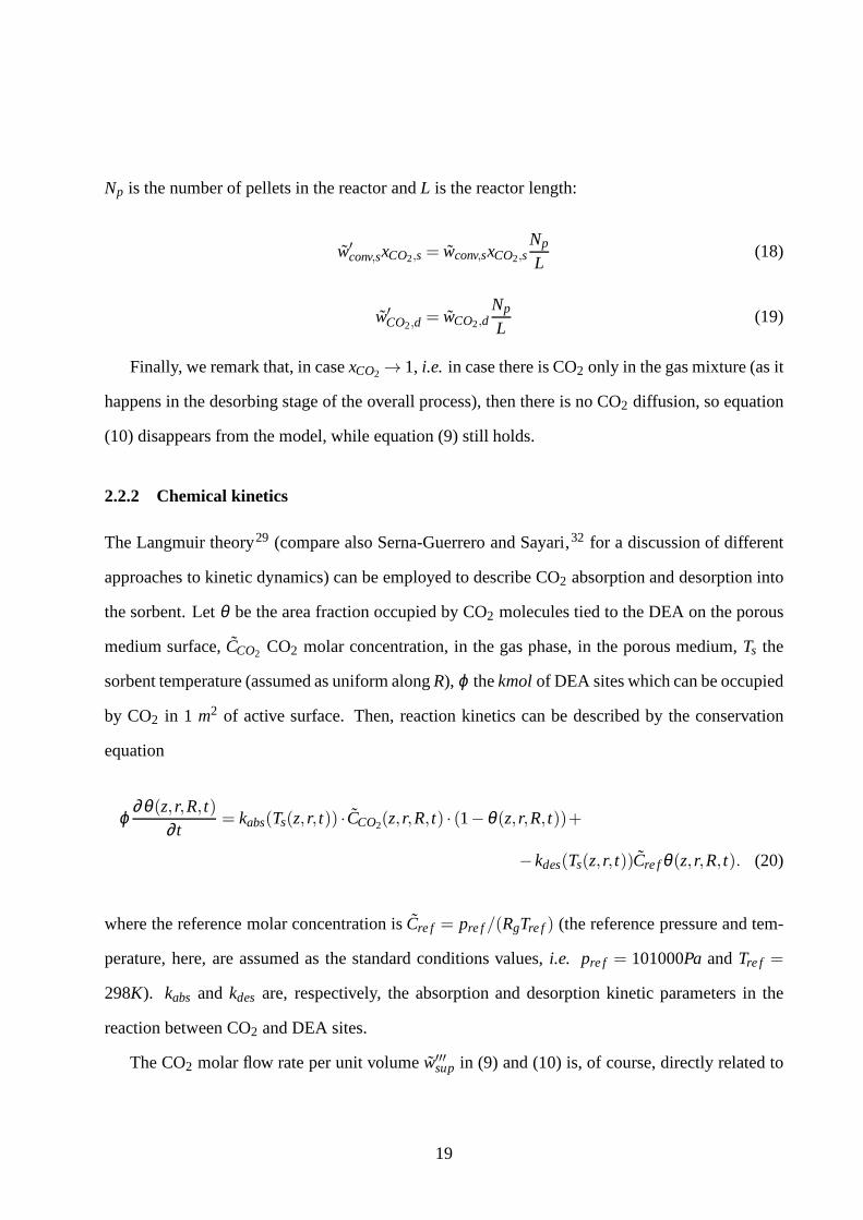
sients provided by our model in 7. As can be seen, the model is able to reproduce the real transients
in all working conditions with satisfactory matching. Model adherence to the system behaviour
could be increased by further improving parameter tuning. Several parameters in the model, in
fact, such as the bulk and the pellet void fraction values, the active surface per sorbent unit volume
and the heat exchange coefficients, have been taken from literature data so far, and thus they are
subject to non-negligible uncertainty.
Remark 1 (Model parameters updating) One of the main problems in the industrial use and
control of the reactor for CO2 absorption/desorption is the constant wear of the reactor during
its life, which may cause the identified model parameters to become obsolete in the long run. In
other words, the model returned by designers when the reactor is built may be no longer valid
after the reactor has been used for a certain period of time. Hence, in principle, the procedure
for parameter estimation should be repeated from time to time when the operating conditions have
been subject to change. The procedure described in this Section, however, has the drawback that
requires specific experiments on the plant and the intervention of qualified personnel to properly
interpret the data. Thus, altogether, this makes the use of this procedure not feasible for the end
user.
In recent years, a new parameter estimation technique, which is called the Two-Stage (TS)
method, has been proposed in the specialized literature with the purpose of facing proper the
issue of model parameters updating.36 Specifically, the TS method is highly automated, so as
to not require the intervention of qualified personnel, and can be easily reused by the end user
whenever the model parameters need to be re-estimated. To betuned for the specific problem
at hand, the TS method requires a reliable physical model of the reactor along with a range of
possible values for the uncertain parameters. Hence, tuning relies on the modeling and parameter
identification previously discussed. Once tuned, from the end user perspective, the TS method
accepts as input the data collected from a simple experimenton the plant in normal operating
32
Figure 7: Experimental data (blue) Versus model output (red): CO2 outlet molar fraction in thethree validation tests
conditions, and returns as output the new estimated values for the uncertain parameters, without
any kind of human intervention. Moreover, the parameter estimates are obtained at very low
computational cost, making the use of TS simple and effective.
The interested reader is referred to A, where more details onthe TS method are given, along
with an example of application to the reactor for CO2 absorption/desorption.
33

5 Conclusions
The dynamics of a CO2 capture process based on amines supported on solid pellets have been
studied, leading to a PDE and an ODE descriptions. The two main uncertain parameters in the
model are the CO2-amine reaction kinetic parameters. We have provided an identification method
based on physical reasoning and a technique for the automatic update of their estimates, which
have proven a good estimation capability with respect to lab-scale experimental data.
The model developed in this work will be employed to study theoperating procedures and
to design controllers of pilot-scale plants where the solidsorbent-anchored amine process is de-
voted to CO2 capture not only from coal combustion flue gases, but also in biogas upgrading to
biomethane.
A The Two-Stage(TS) method for model parameters updating
In this Appendix we briefly describe the Two-Stage (TS) method,36 a new parameter estimation
technique which is specifically tailored to model parameters updating, as discussed in Remark 1.
The method is based on an intensive offline simulation procedure, which analyzes the behaviour
of the physical model we have developed in Section 2 while spanning across a range of parameters
defined from the values estimated by the procedure describedin Section 4. Hence, the TS method
synergically builds up on the findings of this paper.
The method is outlined in A.1, while numerical results for the CO2 absorption/desorption reactor
are reported in A.2.
A.1 Problem setting and description of the TS method
To introduce the TS method, we need rethinking to the model identification problem in a new
perspective. We rely on the physical model introduced in theprevious sections. The uncertainty
can be restricted to the kinetic parameters. Since the ratiokabs/kdescan be considered as a reliable
identified value, we can take thekabs(T) as the unique uncertain parameter. As seen in Section 4
34

(Figure 7), this parameter depends upon the temperature in aquadratic way. Therefore, we can set
kabs(T) = aT2+bT+c (44)
from the beginning. In conclusion, once the parameter vector p = [a b c]′ is determined, then the
plant behaviour is completely described by the model introduced in Section 2. The parameter
estimation problem, then, is that of retrieving the value ofp based on measurements of properly
chosen input/output signals.
The solution of an estimation problem is an estimation algorithm, also called estimator, which is
nothing but a suitable functionf : R2N→ R
3 which maps the measured observations
DN = {y(1), u(1), y(2), u(2), . . . , y(N), u(N)}
into an estimate for the uncertain parameter:
p := f (y(1), u(1), . . . , y(N), u(N)).
In standard approaches, like those based on Kalman filteringor Prediction Error Methods (PEM)
in system identification,37,38 the mapf is implicitly defined by means of some estimation crite-
rion. This, however, poses some difficulties in using these approaches repeatedly (see Garatti and
Bittanti36 for the details).
The TS approach develops along completely different ideas:it resorts to off-line intensive simula-
tion runs in order to explicitly reconstruct a functionf :R2N→R3 mapping measured input/output
data into a parameter estimatep.
To be precise, we use thesimulatorof the reactor to generate input/output data for a number of dif-
ferent values of the unknown parameterp chosen so as to densely cover a certain range of interest.
35

That is, we collectN simulated measurements
DN1 = {y1(1),u1(1), . . . ,y1(N),u1(N)}
for p= p1; N simulated measurements
DN2 = {y2(1),u2(1), . . . ,y2(N),u2(N)}
for p= p2; and so forth and so on, so as to work out a set of, saym, pairs{pi ,DNi } as summarized
Table 8: The simulated data chart as the starting point of thetwo-stage method.
p1 DN1 = {y1(1),u1(1), . . . ,y1(N),u1(N)}
p2 DN2 = {y2(1),u2(1), . . . ,y2(N),u2(N)}
......
pm DNm = {ym(1),um(1), . . . ,ym(N),um(N)}
in Table 8. Such set of data is referred to as thesimulated data chart.
From the simulated data chart, the functionf is reconstructed as that map minimizing the estima-
tion error over simulated data, i.e.
f ← minf∈F
1m
m
∑i=1
∥∥∥pi − f (yi(1),ui(1), . . . ,yi(N),ui(N))∥∥∥
2, (45)
whereF is a class of fitting functions. Shouldf be found, then the true parameter vector cor-
responding to the actual measurements, sayDN = {y(1), u(1), . . . , y(N), u(N)}, can be estimated
as
p= f (y(1), u(1), . . . , y(N), u(N)).
Solving (45) is of course very critical, because of the high dimensionality of the problem:f de-
pends upon 2N variables, normally a very large number if compared to the numberm of experi-
ments. In the TS approach, the resolution of (45) is split into two stages. This splitting is the key
to obtain a good estimatorf .
36

We now describe the two stages. The interested reader is referred to Garatti and Bittanti36 for the
full details.
First stage. The first step consists of a compression of the information conveyed by input/output
sequencesDNi , in order to obtain new data sequencesDn
i of reduced dimensionality. While in the
dataDNi the information on the unknown parameterpi is scattered in a long sequence ofN sam-
ples, in the new compressed artificial dataDni such information is contained in a short sequence
of n samples (n≪ N). This leads to a new compressed artificial data chart composed of the pairs
Table 9: The compressed artificial data chart.
p1 Dn1 = {α
11, . . . ,α
1n}
p2 Dn2 = {α
21, . . . ,α2
n}...
...pm Dn
m = {αm1 , . . . ,α
mn }
{pi , Dni }, i = 1, . . . ,m, see Table 9.
Each compressed artificial data sequenceDni is obtained by fitting asimple black-boxmodel to
each sequenceDNi = {yi(1),ui(1), . . . ,yi(N),ui(N)}, and, then, by taking the parameters of this
identified model, sayα i1,α
i2, . . . ,α
in, as compressed artificial data, i.e.Dn
i = {αi1, . . . ,α
in}.
It is worth noticing that the simple model used to fit the artificial data plays a purely instrumental
and intermediary role. Hence, it is not required to have any physical meaning, nor it does matter if
it does not tightly fit the data sequencesDNi , as long as theα i
1,αi2, . . . ,α
in reflect the variability of
the pi .
Summarizing, in the first stage a functiong : R2N→Rn is found, transforming each simulated data
sequenceDNi into a new sequence of compressed artificial dataDn
i still conveying the information
on pi . The functiong is defined by the chosen class of simple models used to fit simulated data
along with the corresponding identification algorithm.
Second stage.Once the compressed artificial data chart in Table 9 has been worked out, prob-
37

lem (45) becomes that of finding a maph : Rn→ Rq which fits them compressed artificial obser-
vations into the corresponding parameter vectors, i.e.
h← minh∈H
1m
m
∑i=1
∥∥∥pi−h(α i1, . . . ,α
in)∥∥∥
2, (46)
whereH is a suitable function class.
Problem (46) is reminiscent of the original minimization problem in (45). However, beingn small
thanks to the compression of the information in the first stage, the resolution of (46) is not prob-
lematic anymore. One can e.g. resort to Neural Networks and solve (46) by means of the standard
algorithms developed for fitting this class of nonlinear functions to the data.
Use of the two-stage method.After h has been computed, the final estimatorf mapping in-
put/output data into the parameter estimatep is obtained as
f = h◦ g= h(g(·)),
i.e. as the composition ofg andh.
Note that f is constructed off-line, by means of simulation experiments only. However, when a
real input/output sequenceDN = {y(1), u(1), . . . , y(N), u(N)} is collected, the unknown parameter
vector can be estimated asp= h(g(DN)), that is, by evaluatingf in correspondence of the actually
seen data sequence. This evaluation can be easily performedby an automatic device, which can
be used to generate estimatesp whenever it is needed, at very low computational cost and without
any intervention of specialized personnel.
A.2 Application to the reactor model: results
As we have seen, the TS method is based on the execution of intensive simulation trials of the
physical model. This simulation phase is performed offline and need not to be repeated along
the plant life. When data from a new experiments are available, the algorithms builds the new
38

parameter estimates very fast.
We now describe the offline procedure for the tuning of the TS algorithm to the CO2 absorp-
tion/desorption reactor. We also give some simulation results demonstrating the effectiveness of
the approach.
In 4 we estimated the kinetic absorption parameter for the temperaturesT1 = 40◦C, T2 = 60◦C,
T3 = 85◦C:
kabs(T1) = 5.8257×10⁻⁸m/s,
kabs(T2) = 4.6707×10⁻⁸m/s,
kabs(T3) = 4.6105×10⁻⁸m/s.
Starting from valueskabs(Ti), i = 1,2,3, we construct a range of possible values around them as
follows:
0.5kabs(Ti)≤ kabs(Ti)≤ 2kabs(Ti), i = 1,2,3,
In view of expression (44), these bounds onkabsdefine feasible regions for the triple of parameters
p= [a b c]′.
At this point we are in a position to define the simulation experiments we have performed. To be
precise, we have extractedm=2500 random values forp= [a b c]′, ensuring that the corresponding
kabs meet the above bounds.
Correspondingly, we ran 2500 simulations of the reactor, each time injecting a CO2 molar
fraction step of 10% as the input, starting from steady-state conditions at an initial temperature
T = 60 ◦C. As the output signal we have considered temperature at thebeginning of the reactor
(point A in 3). Typical temperature outputs for three valuesof the parameter vectorp are depicted
in Figure 8. By sampling at 0.025Hz the input and output signals, we obtained 2500 input/output
sequences eachN = 150 samples long:
ui(1),yi(1),ui(2),yi(2), . . . ,ui(150),yi(150),
39

0 100 200 300 400 500 600 70058
60
62
64
66
68
70
72
T
t
Figure 8: Typical temperature diagrams at point A (reactor inlet) while injecting an inlet CO2molar fraction step.
i = 1,2, . . . ,2500. These sequences together with the 2500 extracted values for p formed the
simulated data chart.
As for the generation of the compressed artificial data chart, we noticed that, in our experiments,
the output looks like an impulse response, because of the zero in the origin introduced by the
external refrigerator, which forces the temperature to return to the initial value. Hence, by letting
∆ui(t)= ui(t)−ui(t−1) be the impulse corresponding to the given step, we fitted to each generated
data sequence a low-order state-space model
x(t +1) = Fx(t)+G∆ui(t)
yi(t) = Hx(t),
by using the Ho-Kalman algorithm.39 To be precise we have considered a third order system, so
that the total number of entries in the triple(F,G,H) is 15. These entries are the parameters we
have used as compressed artificial dataα i1,α
i2, . . . ,α
i15, i = 1,2, . . . ,2500.
The final estimatorh(α i1,α
i2, . . . ,α
i15) was instead derived by resorting to a feed-forward 3-layers
40
neural network, with 20 neurons in each hidden layer.40 The network weights were trained by the
usual back-propagation algorithm. The order of the state-space model as well as that of the neural
network were eventually chosen by means of cross-validation.
In order to test the TS estimator, we picked 500 new random values for the uncertain vector pa-
rameterp, and correspondingly we ran new 500 simulations of the reactor model in the same
experimental conditions as in the training phase. The 500 data sequences obtained by sampling
input and output signals at 0.025Hz were made available to the TS estimator so as to generate
500 estimates of the parameter vectorp. These estimates were eventually compared to the true
values of the parameter vector so as to evaluate the performance of the obtained estimator (cross-
validation).
In Figure 9, the estimates ˆa, b, and c, respectively, as returned by the TS estimator, are plotted
against the true parameter valuesa, b, andc. That is, with reference, e.g., to the first box at the top,
thex-axis of each plotted point is the extracted value for the parametera, while they-axis is the
corresponding estimate supplied by the TS estimator. The same interpretation holds for the other
figures. Clearly, the closer the points to the graph bisector, the better the estimator.
As it appears, the figures reveal a great estimation capability of the TS estimator, especially as for
parametersb andc, while parametera is less identifiable. Overall, the estimation results are quite
good, and the TS approach was able to produce an explicit estimator mapf (·) = h(g(·)), defined
as the composition of the Ho-Kalman algorithm and the trained neural network, which can be used
over and over to generate suitable estimates ofp whenever a tuning of the reactor model is needed.
Acknowledgement
This work has been financed by the Research Fund for the Italian Electrical System under the
Contract Agreement between RSE S.p.A. and the Ministry of Economic Development - General
Directorate for Nuclear Energy, Renewable Energy and Energy Efficiency in compliance with the
Decree of March 8, 2006. The support by the MIUR national project “Identification and adaptive
41

0.2 0.3 0.4 0.5 0.6 0.7 0.8 0.9 1 1.1 1.20.2
0.3
0.4
0.5
0.6
0.7
0.8
0.9
1
1.1
1.2
0.3 0.4 0.5 0.6 0.7 0.8 0.9 1
0.3
0.4
0.5
0.6
0.7
0.8
0.9
1
0.2 0.3 0.4 0.5 0.6 0.7 0.8 0.90.2
0.3
0.4
0.5
0.6
0.7
0.8
0.9
Figure 9: Estimation results for parametersa, b, andc.
control of industrial systems” and by CNR - IEIIT is also gratefully acknowledged.
References
1. Ciferno, J. P.; Ramezan, M.; Skone, J.; ya Nsakala, N.; Liljedahl, G. N.; Gearhart, L. E.; Hes-
termann, R.; Rederstorff, B.Carbon Dioxide Capture from Existing Coal-Fired Power Plants
[Online]; DOE/NETL-401/110907; DOE/NETL Report, 2007. http://www.netl.doe.gov/File
Library/Research/Energy Analysis/Publications/CO2-Retrofit-From-Existing-Plants-Revised-
November-2007.pdf (accessed September 4, 2014).
42

2. Herzog, H.An Introduction to CO2 Separation and Capture Technologies; MIT Energy Labo-
ratory, 1999.
3. Spigarelli, B. P.; Kawatra, S. K. Opportunities and challenges in carbon dioxide capture.J.
CO2 Util. 2013, 1, 69–87.
4. Veawab, A.; Tontiwachwuthikul, P.; Chakma, A. Corrosionbehaviour of carbon steel in the
CO2 absorption process using acqueous amine solutions.Ind. Eng. Chem. Res.1999, 38,
3917–3924.
5. Serna-Guerrero, R.; Da’na, E.; Sayari, A. New insights into the interactions of CO2 with
amine-functionalized silica.Ind. Eng. Chem. Res.2008, 47, 9406–9412.
6. Knudsen, J. N.; Jensen, J. N.; Vilhelmsen, P. J.; Biede, O.Experience with CO2 capture from
coal flue gas in pilot-scale: Testing of different amine solvents.Energy Procedia2009, 1,
783–790.
7. Goff, G. S.; Rochelle, G. T. Monoethanolamine degradation: O2 mass transfer effects under
CO2 capture conditions.Ind. Eng. Chem. Res.2004, 43, 6400–6408.
8. Herzog, H.J.; Drake, E. M.Long-Term Advanced CO2 Capture Options; IEA/93/OE6; IEA
Greenhouse Gas R&D Programme: Cheltenham, UK, 1993.
9. Zhao, L.; Riensche, E.; Blum, L.; Stolten, D. How gas separation membrane competes with
chemical absorption in postcombustion capture.Energy Procedia2011, 4, 629–636.
10. Favre, E.; Bounaceur, R.; Roizard, D. A hybrid process combining oxygen enriched air com-
bustion and membrane separation for post-combustion carbon dioxide capture.Sep. Purif.
Technol.2009, 68, 30–36.
11. Sjostrom, S.; Krutka, H. Evaluation of solid sorbents asa retrofit technology for CO2 capture.
Fuel 2010, 89, 1298–1306.
43

12. Krutka, H.; Sjostrom, S.Evaluation of Solid sorbents as a Retrofit Technology for CO2
Capture from Coal-Fired Power Plants[Online]; Final technical report; DOE Award
Number DE-NT0005649; Report Number 05649FR01; 2011. http://www.netl.doe.gov/File
Library/Research/Coal/ewr/co2/evaluation-of-solid-sorbents-nov2011.pdf (accessed Septem-
ber 4, 2014).
13. Zhao, W.; Zhang, Z.; Li, Z.; Cai, N. Investigation of thermal stability and continuous CO2
capture from flue gases with supported amine sorbent.Ind. Eng. Chem. Res.2013, 52, 2084–
2093.
14. Samanta, A.; Zhao, A.; Shimizu, G. K. H.; Sakar, P.; Gupta, R. Post-Combustion CO2 Capture
Using Solid Sorbents: a Review.Ind. Eng. Chem. Res.2012, 51, 1438–1463.
15. Gray, M. L.; Hoffman, J. S.; Hreha, D. C.; Fauth, D. J.; Hedges, S. W.; Champagne, K. J.;
Pennline, H. W. Parametric Study of Solid Amine Sorbents forthe Capture of Carbon Dioxide.
Energy Fuels2009, 23, 4840–4844.
16. Mazzocchi, L.; Notaro, M.; Alvarez, M.; Ballesteros, J.C.; Burgos, S.; Pardos-Gotor, J. M.
Preparation and laboratory tests of low cost solid sorbentsfor post-combustion CO2 capture.
Proceedings of the International conference on Sustainable Fossil Fuels for Future Energy -
S4FE2009, Rome, Italy, Jul 6-10, 2009.
17. Notaro, M.; Savoldelli, P.; Valli, C.Tests on Solid Sorbents for Post-Combustion CO2 Cap-
ture and Feasability of a Pilot Application[Online]; Technical report; 2008; in Italian.
http://www.ricercadisistema.it (accessed September 4, 2014).
18. Notaro, M.; Pinacci, P.Carbon dioxide capture from flue gas by solid regenerable sorbents.
Proceedings of the 3rd International Conference on Clean Coal Technologies for our Future,
Cagliari, Italy, May 15-17, 2007.
19. Notaro, M.; Pardos Gotor, J. M.; Savoldelli, P. Method for capturing CO2. 2012; WO Patent
44

App. PCT/ES2012/070,137. http://www.google.com/ patents/WO2012120173A1?cl=en (ac-
cessed September 4, 2014).
20. Notaro, M.Post-combustion CO2 capture by solid sorbents.In Convegno nazionale AEIT
2011, Milan, Italy, Jun 27-29, 2011; in Italian.
21. Bittanti, S.; Calloni, L.; De Marco, A.; Notaro, M.; Prandoni, V.; Valsecchi, A.A process
for CO2 post combustion capture based on amine supported on solid pellets. Proceedings of
the 8th IFAC International Symposium on Advanced Control ofChemical Processes, Furama
Riverfront, Singapore, Jul 10-13, 2012.
22. Finlayson, B. A. Packed bed reactor analysis by orthogonal collocation.Chem. Eng. Sci.1971,
26, 1081–1091.
23. Santacesaria, E.; Morbidelli, M.; Servida, A.; Storti,G.; Carrà, S. Separation of Xylenes on
Y Zeolites. Note II: Breakthrough Curves and Their Interpretation.Ind. Eng. Chem., Process
Des. Develop.1982, 21, 446–451.
24. Bisone, L.; Bittanti, S.; Canevese, S.; De Marco, A.; Garatti, S.; Notaro, M.; Prandoni, V.
Modeling and parameter identification for CO2 post-combustion capture by amines supported
on solid sorbents.Proceedings of the 19th IFAC World Congress, Cape Town, South Africa,
Aug 24-29, 2014.
25. Foo, K. Y.; Hameed, B. H. Insights into the modeling of adsorption isotherm systems.Chem.
Eng. J.2010, 156, 2–10.
26. Ruthven, D. M.Principles of Adsorption and Adsorption Processes; John Wiley & Sons: New
York, 1984.
27. Ruthven, D. M.; Farooq, S.; Knaebel, K. S.Pressure Swing Adsorption; VCH: New York,
1994.
28. Bird, R. B.; Stewart, W. E.; Lightfoot, E. N.Transport phenomena; Wiley: New York, 1960.
45

29. Froment, G. F.; Bischoff, K. B.Chemical Reactor Analysis and Design, 2nd ed.; John Wiley
& Sons: New York, 1990.
30. Balakrishnan, A. R.; Pei, D. C. T. Heat Transfer in Gas-Solid Packed Bed Systems. 1. A
Critical Review.Ind. Eng. Chem., Process Des. Develop.1979, 18, 30–40.
31. Mason, E. A.; Malinauskas, A. P.; Evans III, R. B. Flow andDiffusion of Gases in Porous
Media.J. Chem. Phys.1967, 46, 3199–3216.
32. Serna-Guerrero, R.; Sayari, A. Modeling adsorption of CO2 on amine-functionalized meso-
porous silica. 2: Kinetics and breakthrough curves.Chem. Eng. J.2010, 161, 182–190.
33. Mahan, B. H.University Chemistry, 3rd ed.; Addison-Wesley Publishing Co.: Reading, 1975.
34. Barrow, G. M.Physical Chemistry, 5th ed.; McGraw-Hill: New York, 1988.
35. Atkins, P. W.Physical Chemistry, 5th ed.; Oxford University Press: Oxford, 1994.
36. Garatti, S.; Bittanti, S. A new paradigm for parameter estimation in system modeling.Int. J.
Adapt. Contr. Signal Process.2013, 27, 667–687.
37. Ljung, L.System Identification: Theory for the User, 2nd ed.; Prentice-Hall: Upper Saddle
River, 1999.
38. Söderström, T.; Stoica, P.System Identification; Prentice-Hall: Englewood Cliffs, 1989.
39. Ho, B. L.; Kalman, R. E. Effective construction of linearstate-variable models from in-
put/output functions.Regelungstechnik1966, 14, 545–592.
40. Haykin, S.Neural Networks: A Comprehensive Foundation, 2nd ed.; Prentice Hall: Upper
Saddle River, 1998.
46