a pollution trading system with cost assymetryageconsearch.umn.edu/bitstream/103719/2/a pollution...

A Pollution Trading System with Cost Asymmetry

An Application to Nonpoint Source Trading in the Boone River

Watershed

Adriana M. Valcu

Center for Agricultural and Rural Development and

Department of Economics

Iowa State University

Email: [email protected]

Catherine L. Kling

Center for Agricultural and Rural Development and

Department of Economics

Iowa State University

Email: [email protected]

DRAFT PLEASE DO NOT CITE!

Selected Paper prepared for presentation at the Agricultural & Applied Economics Association’s

2011 AAEA & NAREA Joint Annual Meeting, Pittsburgh, Pennsylvania, July 24-26, 2011

Copyright 2011 by Adriana M. Valcu and Catherine L. Kling. All rights reserved. Readers may

make verbatim copies of this document for non-commercial purposes by any means, provided

that this copyright notice appears on all such copies.

Draft‐Please do not cite!

1

Abstract

The goal of watershed scale analysis is to assign to each field unit the best set of

agricultural practices in order to achieve a maximum outcome from both environmental and

economic perspectives. Watershed physically based models linked to multiobjective optimization

models can overcome the high dimensionality of watershed pollution problem. Market based

instruments such as permit trading settings which consider abatement measures’ cost

heterogeneity have been regarded as being superior to command and control programs.

Empirical analysis reveals that when local environmental authority and farmers have different

cost information, a permit trading program has the potential to offer cost savings.

Key words: cost asymmetric information, command and control program, evolutionary

algorithms, nonpoint source pollution, water quality trading


2

1.1.General overview

Water quality impairments have been created as a result of both modern agriculture and

urban activities. Over time, the measures taken under the Clean Water Act have succeeded in

reducing many point source emissions, but currently, non point emissions and agricultural

emissions are the most significant contributors to water quality problem in the United States

(EPA,2003). The latest National Summary of State information indicates that more than 50% of

the 26% of nationwide rivers whose water quality have been assessed are inadequate to support

wildlife, fishing and recreational activities. The same survey states that more than half of wetland

nationwide areas have been impaired by agricultural activities.

Market based instruments such as permit trading programs have been regarded as

successful instruments for a broad range of environmental problems such as air pollution control,

habitat protection and resource compensation. Based on the historical achievements of the Acid

Rain Program that used tradable permits for sulfur dioxide emissions, market based instruments

have been proposed to address water quality pollution. Point-nonpoint source trading systems, by

requiring a mandatory participation of the point sources and a voluntary participation of the non

point sources have the potential for achieving the proposed caps on point source emissions at

lower cost, but there have not been a large number of trades or documented successes of these

programs. Following the EPA beliefs that "market based approaches to water quality trading

provide greater flexibility and have the potential to achieve water quality and environmental

benefits greater than would otherwise be achieved under more traditional regulator approaches"

(EPA 2003), designing and enforcing a trading system that encourage emission trading among

non point sources might be a solution for the current state of water quality pollution.

1.2. Literature review

In the following section.We outline a brief review of water quality trading literature,

focusing on the literature that directly relates to nonpoint –nonpoint trading.

The basic idea behind a permit trading system is not complicated. In order to reduce the

amount of pollution, the regulator, an environmental agency, determines a total standard to be

implemented and the number of permits to be given to the polluters. Permits can be freely traded.


3

A polluter's total emissions cannot exceed the amount allowed by the number of permits held at a

given moment. The permit price is the result of market equilibrium forces. Following Coase’s

(1960) argument that if the property rights are well defined and transferable, the market forces

give the best use of the resources, Crocker (1966) and Dales (1968) provided the first theoretical

models of tradable permits for air pollution, and water pollution, respectively. The experience

with the sulfur dioxide trading program brought the idea of using tradable permits as a solution

to the water quality impairments (Colby, 2000).

Most research to date has been focused on modeling trading systems that include either

only point sources or both point and nonpoint sources (Montgomery 1972, Krupnick et al, 1983,

Shortle and Abler, 1997;Hung and Shaw 2005). Much attention has been given to the size of

“diffusion” or “delivery coefficients”. Delivery or diffusion coefficients are used to define the

impact of one unit of emissions to the total ambient pollution, where ambient pollution refers to

the pollution concentration measured in stream as opposed to emissions at the source of the

pollution, such that edge -of--field. The total ambient pollution, , or the damage function

is defined as a function of individual emissions, and delivery coefficients, . The trading ratio,

the central element of a point point or point non point emissions trading, is defined by the

delivery coefficients. Earlier theoretical approaches assumed that diffusion coefficients are fully

determined and that the pollution damage function is a convex combination of individual

emissions weighted by the delivery coefficients (Montgomery, 1972). Hung and Shaw (2005)

use trading ratios defined by the delivery coefficients to design a zonal permit trading system

able to achieve water quality goals in a least cost manner. At the same time, Montgomery

recognized that assuming a linear combination can impose significant limitations on the viability

of permit trading market. In the context of water quality trading, the majority of existent market

transactions use delivery coefficients as proxies for trading ratios (USEPA, 2004) and most

pollution reductions are based on the delivery coefficients, thus the efficiency of any policies

depends on their accuracy.

In the watershed, agricultural activity is the main source of water pollution, with many

potential pollution sources, and an equal number of delivery coefficients to be estimated.

Theoretically, one would need to estimate a number of delivery coefficients equal to the number

of polluting sources in the watershed. Of course, empirically this would be cumbersome and


4

almost impossible to enforce, hence it would be feasible to divide the watershed in a number of

smaller subwatersheds and estimate a diffusion coefficient for each of them. Estimating delivery

coefficients may be a daunting task, but is essential for achieving sound policy. Furthermore the

delivery coefficients are site specific, but lessons can be learned about their characteristics and

the techniques employed in their estimations.

Previous studies assumed that delivery coefficients can be estimating using information

related by source characteristics such as slope, soil characteristics, distance to the water body,

and agricultural practices (Carpentier, Bosch and Batie, 1989) or the practices used on the sites

that are located down slope of a particular slope. Khanna et al. (2003) assumes that the

contribution of each site emissions is determined by two factors. The first factor is a trapping

coefficient that depends not only on the site characteristics and agricultural practices used but

also on the characteristics and land use practices of the sites located upslope. The second

coefficient is a sediment transport coefficient that determines the onsite emissions that adds up to

the emissions measured at the offsite receptor point. The authors state that the relationship is too

complex to be exogenous, and that an endogenous treatment is required. Consequently, the

diffusion coefficients of one source are influenced by its own characteristics but also by the

upslope and down slope sources' characteristics and land use practices.

There are not many studies in the context of trading water quality that approach

agricultural non point sources only. This is partially due to the fact that nonpoint source

emissions are considered difficult to measure and monitor, making it difficult to link the

agricultural production function to the ambient pollution measured at the receptors (Morgan et

al., 2000).

Morgan, Conggins and Eidman (2000) describe a marketable permit trading scheme able

to manage nitrate pollution of groundwater supplies for rural communities with intensive

agricultural activity. The level of nitrate leaching is measured at the level of drinking water well.

The authors use soil and groundwater transportation models to predict nitrate leaching rates from

a particular crop area. According to their model each farm is made accountable for its emissions

to a given water well, hence nonpoint source emissions are transformed into point source

emissions. Their model takes into account that the farm's potential to contribute to total ambient


5

pollution depends on its location. The permit trading system is defined as an ambient permit

system, defined in Montgomery sense, where farms are allowed to emit up to a certain level1.

Three integrated models: production, soil, and groundwater represent the foundation of

the permit trading model. The permit trading model is designed for trading nitrate emissions. The

production model defines the profits as a function of yield, where yields are defined as a function

of the fertilizer, agricultural practices and rotations. The abatement cost is defined as the

difference in profits before any regulation is imposed and the profits after regulations are

adopted. The farm minimizes its abatement costs, where the cost is defined as the sum of the loss

profits and the expenditure on permits. By selling permits the compliance cost is more likely to

decrease.

In implementing the trading system the authors underline the importance of the time

framework and of the baseline. Estimating the transfer coefficients, the marginal abatement cost,

and initial permit allocation are also considered to have an important role in the trading scheme.

Marginal abatement costs are defined as the change in the nitrate levels at the well due to a shift

in the agricultural practice. The allocation of permits is made at the beginning of the planning

period. The equilibrium price is determined through repeated auction, the amount of abatement

and the trading decision is made by comparing the equilibrium price with the marginal abatement

cost. The abatement cost is higher to the farms whose emissions have the greatest impact on the

water quality measured at a specific well.

Prabodanie et al. (2010) propose an offset tradable permit system as a solution to non

point source water pollution, focusing on nitrate loadings on an aquifer. They use the same

approach followed by Morgan et al. (2000), but in addition run several simulations regarding the

trading outcome. The trading is overseen by a central authority that via an auctioning procedure

determines the clearing price for the permit trading market. Their findings confirm that farmers

are better off by being allowed to trade than when a command and control program is in place.

For example per farm average profits increased by almost 10 % in when trade is allowed.

1 In an ambient permit system, the permits are denominated in emissions measured at the receptor point, rather than emissions measured at the edge-of-field.


6

1.3. Ancillary literature review

In addition to building on previous literature in nonpoint emission trading, we will use a

number of models and tools. In this section, we will provide a short description of these tools.

Difficulties in establishing a direct link between the agriculture activity and ambient

pollution level measured at receptors, where each source is made liable for its discharges, have

been one of the main impediments in the development of a trading system that approaches

agricultural nonpoint sources. Better understanding of the interactions between agriculture

activity and water quality has been achieved with development of hydrological model.

Soil and Water Assessment Tool

The Soil and Water Assessment Tool (SWAT) is a complex water quality watershed

based hydrological model developed by the US Department of Agriculture to simulate the impact

of point and nonpoint source emissions (Arnold et al (1998); Arnold and Fohrer (2005), and

Gasmann et al. (2008)). The model is designed to run watershed simulations based on a wide

range of inputs such as: climate data (precipitation, temperature, etc.), soils characteristics

information (slope, soil quality, topography, erosion, etc.), plant growth and crop rotations,

nutrient management, nutrient transport and transformation, and land use and management

practices. Using the above data as input, SWAT outputs consist of in stream concentration

estimates for nitrogen, phosphorous and sediment loadings. The output provides overall

measures of the concentrations, as well as detailed information about the components of each

type of discharges. For example, for nitrogen loadings, we can retrieve detailed information

about components of nitrogen loadings. The obtained information can be used to predict

watershed loadings on wide time range, from daily to annually based estimates.

The SWAT model is used to estimate the changes in nutrient loadings as a response to

alternative conservation practices under different crop choices and rotation alternatives. In order

to run simulations, the watershed, a well-defined geographical entity is divided into several sub

watersheds or sub basins. In SWAT, each subwatershed is delineated further into small

hydrological response units (HRU). An HRU is a conceptual entity, with no precise spatial

location within the subwatershed. It is identified as a percentage area in the subwatershed with

homogenous soil, land use and management practices. The primary water and loading

simulations are made at the HRU level. The estimated loadings can be interpreted as edge-of-


7

field run off emissions. The nutrient loadings measured at the final outlet located at the base of

the subwatershed are obtained by adding the loadings corresponding to each HRU that

previously have been routed through a network of channels and reservoirs.

The development of hydrological models like SWAT, calibrated with watershed specific

data, makes possible the simulation of impact on water quality of different watershed scenarios.

A watershed is divided in hundreds of fields, and each field may have multiple agricultural

practices that are suitable for its type of soils. For example, for a set of nine agricultural practices

and 2900 fields, the total number of possible watershed scenarios is 9 possible scenarios.

Using SWAT, a water quality level can be estimated for each watershed configuration. With

appropriate economic data the cost of agricultural activity associated with a particular scenario

can be assessed. The question arises: which of those scenarios is most desirable from a cost

and/or pollution reduction perspective? Unfortunately, the high dimensionality of the problem

makes finding a solution through traditional optimization tools practically impossible.

Evolutionary algorithms

One way to deal with the combinatorial nature of the watershed simulation-optimization

model is the implementation of an evolutionary algorithm. Evolutionary or genetic algorithms

(EA) are designed to mimic biological evolution, considered by Mitchel (1996) to be ''in effect,

.a method of searching for solutions among an enormous set of possibilities". Genetic algorithms

are heuristic global search algorithms that are able to find the nearly optimal solution by using

principle like "natural selection" and "survival of the fittest". The first studies that use EAs for

finding the “nearly optimal” solution for conservation practices best placement were published

only in the early 2000s, even though the theoretical background for evolutionary computation

started at the beginning of the 1950s.

The main terminology used in defining EAs is similar to that used in biology, and

consists in terms such as: population, genome, individual, allele set, offspring, recombination,

mutation, etc. Next, we are going to give a brief description of this terminology in the context of

watershed optimization context. The terminology definitions closely follow the one used by

Rabotyagov (2007).

A population is defined by the individuals that share the same defining elements or

characteristics. The genome or the chromosome represents the set of elements that defines an


8

individual. A gene or allele can have several properties. The collection of all properties defines

the allele set that is the same for entire population (i.e. all individuals have the same number of

genes). Each individual of the population is defined by a unique combination of genes and the

properties from the allele set. The evolutionary process assumes a continuous and dynamic

process where the fittest individuals become parents and are able to pass their genes to off

springs by the mean of crossover. The resulted off springs may suffer mutation with a given

probability. The newly created individuals define the new generation or population. The

evolutionary process can span over an unlimited number of generations.

In our case, an individual represents the watershed. A gene is represented by a field, thus

the total number of fields defines the genome. The fields’ properties are defined in terms of the

agricultural practices available in the watershed. The set of all agricultural or conservation

practices defines the allele set. Hence, an individual is defined by a particular combination of

fields and the conservation practices. It represents a possible solution to the pollution cost

minimization problem, where as a population represents the set of all potential solutions to the

same problem. The goal of the evolution process is to find the watershed configuration that

ccount only N reductions and disregard P reductions. Second,r given a budget achieves the

lowest level of ambient pollution.

Genetic or evolutionary algorithms can successfully handle optimizations problems that

have (i) a large space whose characteristics are not well known or have complex properties such

as non convexities and discontinuities, (ii) are complex, and (ii) a solution near global is

acceptable. There are many reasons that make watershed pollution management suitable area for

the use of an EA. First, there are measurement errors in the conservation practices’ abatement

efficiency, second a watershed is defined by hundreds of fields, with each field having more than

one conservation practice available, and most of the cases and realization of ambient pollution

target on average is considered sufficient.

When water quality optimization is considered with respect to a single pollutant, the

optimization problem can be defined as single objective optimization problem. In most of the

cases, water quality impairment is not limited to a single pollutant; hence the optimal solution

requires solving a multi objective optimization problem. In some cases, genetic algorithms can

accommodate this by combining competing multi objectives into a single known objective

function and the solution yields a single optimal solution. In the cases when a single objective


9

function cannot be determined, the solution to a multi objective optimization will consist of a set

of solutions, or a Pareto frontier optimal set. This set is a "near-optimal" set that reveals the

tradeoffs between the different objectives. The near optimal characteristics come with the

“temporal” aspect of the algorithm. More precisely, since there is no clear stopping criteria the

solutions can always improve if more generations are allowed to survive. The solutions are

optimal given the generations number that survived.

Earlier applications of EAs to watershed management focus on a single objective

function, either pollution reduction effectiveness or cost (Srivastava et al; 2002), or on sequential

optimization of effectiveness and cost (Gitau et al; 2004;Veith et al; 2003), where optimization is

made in stages. Bekele and Nicklown (2005) use a multi objective function, but the set of

agricultural practices is limited to crop management practices. Maringanti, Chauby and Popp

(2009) provide a recent application of an EA for a watershed scale optimization problem, with

two conflicting objectives simultaneously: a cost increase and pollution reduction. The set of

conservation practices consists of 54 different combinations. Three different nonpoint pollutants

are considered: phosphorus, nitrogen and sediment but only one pollutant is considered at time,

hence three different optimization models were estimated. For each model, a Pareto frontier

depicts the tradeoff between the two objectives. The allocations of conservation practice in the

watershed according to the optimization results are shown to be superior to random allocation,

resulting in 33 % reductions in sediment loading, 32 % nitrogen loadings and 13% phosphorus

loadings.

I use an EA application developed by Rabotyagov (2007). He considers the cost

effectiveness of joint pollution reduction. Specifically, two pollutants, nitrogen and phosphorus,

are considered simultaneously. As a consequence, the Pareto frontier is three dimensional,

depicting the tradeoff between two different pollutant reductions and cost. The fact that one

conservation practice often has the potential to reduce more than one pollutant provides a solid

reason for this joint approach. Next,we provide a brief description of the particular multi

objective evolutionary algorithm (MOEA) implemented by Rabotyagov (2007) that was used to

obtain the numerical results.

The MOEA is a modification of the Strength Pareto Evolutionary Algorithm2 (SPEA2),

proposed by Zitzler and Thiele (1999). The search process starts by creating a random population

of possible solutions. The random population plays the same role as starting values do in


10

ordinary optimization routines. Individuals undergo a process of mutation, crossover and

ultimately selection. An objective function is evaluated for each individual.

The selection is made based on a fitness score. The fitness score of each individual i in

the population takes into account the number of individuals that are dominated and the number

of individuals that dominates individual i. The degree of ''crowding" around individual i is a

measure of diversity in the population. A lower fitness score implies the individual is closer to

the Pareto frontier and a zero value implies that the individual is on the frontier. Next,we give a

brief description of the algorithm’s principles.

Two types of populations are required at a given time t: the original population, , and a

temporary, or storing population, . At the time t=0, is generated by randomly assigning

individuals with different values from the allele set. These individuals play the same role as

choosing starting values in any other optimization problem. The temporary population is empty

at time zero. It will be populated with individuals created by crossover and mutations. A fitness

value is calculated for each individual from and, sets. In order to determine the fitness

value, each individual is compared with all other individuals. For example, take two individuals

A and B, then individual A is said to dominate in Pareto sense, individual B, if all its genes have

better values. In this case, individual B is said to be dominated. Strength value is a metric

measure that defines the number of individuals that an individual dominates. An individual i

can dominate some individuals but can be dominated by other individuals. Another metric

measure, the raw fitness is obtained by summing the strength values of individuals that

dominate. The raw measure is also a metric of the likelihood of individual i to generate off spring

that pass his characteristics to next generations. If its raw measure is high, this means that it is

dominated by many individuals and less likely to survive, hence it is desirable that the raw

measure to be as closest to zero as possible. A non dominated individual is an individual with

zero raw value.

The searching process can create individuals that do not spread uniformly over the search

space. Some of them tend to cluster into certain areas, leaving some others areas sparse. The

metric measures defined above do not provide any information about the degree of clustering.

Another two metrics measures are defined to incorporate information about clustering around

certain areas of the search space. One of the measures differentiates among individuals that are

too close one to another; the second measure preserves the diversity in the search space by


11

rewarding the individuals that are further away on the frontier. The resulted individuals will be

more uniformly spread over the search space

2. Model

In this this section ,we study the efficiency of a tradable performance standard for water quality

in a watershed area where agriculture activity is the main source of water quality impairment.

We assume that the environmental authority decides to monitor and enforce a cap on the total

level of ambient pollution. The ambient pollution level is monitored at single receptor located at

the watershed exit. The authority identifies a set of conservation or abatement practices that have

been demonstrated to reduce the amount of agricultural discharges from fields (i.e. conservation

tillage, cover crops, reducing the fertilizer application rate and land retirement). Adopting a

conservation practice imposes costs on the farmers in the watershed. Next,we assume that using

available cost information together with an evolutionary algorithm and a complex biophysical

model, the authority is able to identify the optimal placement of conservation practices across the

watershed. The optimal solution is designed to achieve the environmental cap in the least cost

way.

Two alternatives program are considered for enforcing the ambient pollution cap:

command and control and a tradable performance standard program. Assuming away the issues

related to legality of enforcement, we first show that the two approaches will have the same

outcome if the environmental authority has perfect information on the cost of adopting

conservation practices (i.e. abatement costs). In reality, abatement costs are heterogeneous across

farmers and locations and it is unlikely that the authority has the cost information for each farm

in the watershed.

Next,we examine the efficiency of a command and control versus a tradable performance

standard; first under perfect cost information, then under asymmetric cost. In the case of a

command and control program, the farmer is constrained to adopt a specific conservation

practice, regardless of whether an alternative practice could achieve the same emission

reductions at a lower cost. In this chapter we show that, a more efficient solution would be a

tradable performance based program, where farmers are allowed to choose the abatement or

conservation practice that works best for them as long as the total discharges satisfy a pollution


12

standard. The tradable pollution standard can be either an emission based standard (i.e. measured

at the field edge) either an ambient based standard (i.e. measured at the outlet of watershed).

Consider a simple model of pollution where a watershed is impaired by agricultural

runoff consisting of nitrogen and phosphorus. My model follows uses similar notations as the

model presented by Shortle and Abler (1997).

There are F farms in the watershed. The farms are heterogeneous from the point of view

of soil characteristics, ambient pollution contributions and abatement costs. The ambient

standard is monitored at the outlet, located at the base of the watershed. Run off pollution is an

externality associated with conservation activity. Let , the ith farm's contribution measured at

the edge of the field, be defined as:

, ∀ 1, . . . , (2.1)

Where is a Jx1 vector of J’s conservation practices available to farm i, and represents

the farm's idiosyncratic characteristics such that soil type, corn suitability rate, slope. Hence, the

edge-of-farm emissions are influenced by two factors: the choice of the conservation practice,

and the farms characteristics.

Farms are considered to be decision making agents that maximize profits; they are price

takers both in output and input markets. The baseline edge-of-field emissions are the result of

this maximization behavior absent any regulations on the pollution levels.

A water quality production function, , measures the total ambient pollution

monitored at the main outlet . The function is defined in terms of each farm’s individual edge-of-

field emissions, described by the vector . Location and the agricultural activities of the

surrounding farms are other factors that enter in the ambient pollution function. In reality, the

water quality function is unlikely to be known given the complexity of the agricultural and

hydrological process that take place in a watershed and is assumed to be a highly non linear and

non differentiable function of individual edge of-field emissions.

Most economics studies assume that the damage function is a linear combination of each

source weighed by its delivery coefficients (also known as diffusion or dispersion

coefficients).The terminology was introduced by the empirical economics literature that studies

trading system as instruments to implement water quality policies (Montgomery, 1972). In this

study, we assume that the water quality production function is known and can be expressed as an


13

exact combination of delivery coefficients and edge of field emissions. This is equivalent to

assuming that there edge-of-fields discharges can be determined free of measurement errors.

∑ (2.2)

where is the delivery coefficient for source i, measure the amount of edge of field

nutrient loading that reaches the main outlet2.

One of the objectives is to study the change in farmers’ behavior under an imposed

cap, ,on the total ambient pollution relative to a command and control solution. Abatement

costs are defined as the difference between baseline profits and the profits associated with less

polluting production activity3. The cost can be defined as a function of the conservation practice

and an idiosyncratic parameter , that accounts for the fact that adoption costs vary by location

due to differences in physical characteristics of the farm (i.e., soils, slope, etc.), location and

farms’ management abilities.

; ∀ 1, … , (2.3)

I assume that individual farmer knows the cost of adopting a conservation practice. The

environmental authority cannot access cost information at farm level, but rather can infer

information about the distribution of the costs. The first best solution is defined as the least cost

solution when at a cap is imposed on the total level of ambient pollution and the regulator has

complete information about the conservation costs. In what follows, the first best solution is

contrasted with the solution obtained in the case where the regulator knows only the distribution

of the costs across the farmers.

Command and control program

The environmental agency decides to enforce a cap on total ambient emissions, . It

seeks to minimize the expected abatement cost of all farms across the watershed such that the

total expected ambient emissions are less than the ex-ante established cap.

∑ , . ∑ (2.4)

The Lagrangian is given by :

∑ , ∑ , (2.5)

2 To simplify, I drop from , with no consequence on the results’ derivation. 3 Alternatively, assuming risk neutrality, the abatement costs represent the farm’s willingness to accept to implement a conservation practice


14

The optimal solution, ∗ , must satisfy:

∗ ∑ ,

∗ 0,

∗ 0 (2.6)

0

∗ 0 (2.7)

If ∗ 0, i.e. the conservation practice is chosen, then the first order condition is equal

to zero. The second equation is for , the shadow price of the environmental constraint.Assuming

that an interior solution exists, the following result will emerge:

∗ ∗ ∗

∗ ∀ 1, … , (2.8.)

Where ∗ gives the optimal amount of discharges associated if conservation practice is

chosen.

Equation (2.8) states that the marginal abatement cost is equal to the product of the

shadow price of the pollution constraint multiplied by the marginal reduction in edge-of-field

emissions due to conservation practice

Under perfect information, the environmental authority would assign for each farm an

optimal plan consisting of the placement of optimal conservation practice, ∗ , and thus

implicitly an optimal amount of edge of field pollution ∗, ∀ 1, … , farms and ∀ 1, … ,

available conservation practices. The optimal choices can be used to implement either a

command and control program or an ambient standard program. In this case, since the ambient

pollution function is assumed to be a linear function, in the case of command and control

programs, farms might be asked to limit their ambient emissions to ∗ by implementing the

∗ , as abatement practice, or in the case of an ambient standard program, farms are able to

choose the conservation practice as long as their edge of field discharges do not result in a

violation of their performance standard ∗ .

Total abatement cost, denoted by ∗ is obtained by summing the cost of adopting the

conservation practices for all farms across watershed.

∗ ∑ ∗ ∗ , (2.9)


15

Tradable ambient standard program

Assuming that the true form of water quality function is a linear function of edge of field

discharges weighted by known and well defined delivery coefficients, the social optimal solution

can be implemented under a command and control system where specific conservation practices

are prescribed for each location. Alternatively,we can consider a tradable performance standard

setting, where each farm has the freedom to choose its own conservation practices, but its

emissions are constrained by an individual pollution standard. In both cases, the water quality

target is achieved at the least cost solution.

Now, assume that the authority decides to implement an ambient standard for each farm.

Given that the set of conservation practices is the same, farm minimizes the abatement cost

( such that the ambient emissions are less or equal to the cap imposed by the environmental

agency.

min ∈ , (2.10)

. , ∗ (2.11)

The optimality conditions, , are given by, in the case of an interior solution,

(2.12)

Where, is the individual shadow price of ambient pollution, quantifying the

incremental increase (decrease) in cost if the ambient standard is more (less) stringent

Assuming perfect information, optimal solution and performance standard solution are

equivalent, ∗= . This implies:

∗ ∗

∗

∀ 1, … , (2.13)

Hence, λ∗ λ that optimal individual shadow prices must be the same across

watershed.

Total cost of a tradable performance standard program is defined as:

∑ , (2.14)

If there is perfect information and if the water quality production function is a linear

function of the edge- of-field discharges and well defined delivery coefficients, then total cost of

the two programs will be same, and the ambient target will be realized in the least cost way.


16

Achieving the first best under cost asymmetry

In reality, given the idiosyncratic nature of conservation cost, environmental authority

does not have the same level of cost information as farms do, instead it can only infer some

estimates of the distribution of the true costs referred as: . In this case, the best the authority

can do is to consider the second best problem:

∑ , . ∑ (2.15)

where represents a vector of the mean costs of the J conservation practices.

The solution to this problem will generally differ from that obtained in (2.1) and the

assignment of abatement practices, , will not necessarily coincide with the least cost solution,

∗. Likewise, the edge-of-field emissions, ), will be different from the first-best, ∗. Total

costs are given by:

∑ , (2.16)

Under a command and control implementation system, the solution imposed by authority,

), may not reflect the least cost allocation of conservation practices since some farms may

have much lower or higher costs than the mean, which, if known by the authority, could be used

to more cost-effectively assign practices to fields. Nonetheless, the overall abatement target, ,

will be met

In this case, the authority can increase social welfare relative to a command-and-control

assignment of conservation actions, , by allowing firms to meet a performance standard,

. Since firms know their true costs, they may be able to meet the performance standard

allocated to them less expensively by using a different conservation practice (or combination of

practices). If faced with a performance standard, firms will face the following optimization

problem,

, . , (2.17)

The farmers minimize the abatement costs given the true costs, subject to a performance standard

based on average estimates of true costs. The solution is given by , and the

corresponding costs:

∑ , (2.18)

The magnitude of cost savings under asymmetric cost information is given by the

difference between total costs under and total cost under , … , ; defines the vector


17

of field level stock. Since optimal placement of conservation practices can be different under the

two cost sets and the costs set are different, a direct comparison of the two total costs is not

feasible. In order to make the costs comparison, the solution of the environmental agency needs

to be reevaluated at the set of costs used in individual optimization The size of the cost savings,

∆ , if any, is be given by:

∆ ∑ , ∑ , (2.19)

Where ∑ , represents the total cost of a command and control program whose

solution given by equation (2.16) is re-evaluated at the true set of costs, .

Another comparison that can be made is the difference between the total cost of a

command and control program under a cost set defined and total costs when the same outcome

evaluated at the set of true costs, . The difference can be interpreted as how much would a

command and control program designed with cost if the true costs are given by ; it represents

the extent to which the regulator underestimates or overestimates the overall costs of the

program.

∆ ∑ , ∑ , (2.20)

3. Data and methodology description

Next,we provide a description of data and methodology used to generate the empirical

evidence for cost the savings given by equation (2.19) and (2.20).

Study area

The study area is represented by a watershed located in the north central part of Iowa, the

Boone Watershed River (BWR). The watershed covers more than 237,000 acres in six counties.

The watershed area is crop intensive, with corn and soybean representing almost 90% of the

agricultural activity. The surface area had been intensively tile drained, as a consequence the

wetlands area had been reduced significantly. Moreover, the Boone watershed agricultural area

has been found responsible for some of the highest nitrogen loadings among Iowa’s watersheds

(Libra et. al 2004).

Land use in the watershed is dominated by agriculture: with 89.7% of the area

representing crop land, 5.6% of the area representing retired land, 2.6% forestry area and the rest

of the area accounting for urban areas and water surfaces. Most of the land is flat area,


18

characterized by soils with low slopes, i.e. 73% of the areas have the length of the slope less than

0.01 inches. Slope characteristics are relevant to our analysis in two ways. First, the size of the

slope affects the choice of the conservation practices. Second, it affects the total discharges

associated with a particular area. Corn suitability rating is another characteristic that defines the

potential yield4. CSR is an index that ranges between 0 and 100, where high values are

associated with high quality soils. A soil with a high CSR value is less likely to have high rates

of fertilization, and at the same time is less likely to be considered for land retirement as a

solution for reducing the nitrate loadings. In the BWR more than 50% of the soils have been

rated with CSR values ranging 50 to 79 and for 40% of the soils have CSR values higher than 80.

The required data for modeling system (i.e. SWAT mode) was collected at Common

Land Unit level (CLU)5. More than 16,300 CLUs have been identified in the BWR. As HRU is

the unit required by SWAT model, the CLUs were regrouped in roughly 2,900 HRU. Data about

crop rotation, land use, fertilizer management, tillage and conservation practices were provided

by a field level survey conducted by Kiepe (2005).

Conservation practices

The set of conservation practices selected as abatement practices for achieving the

nutrient loading standards includes: reducing the rate of fertilizer application, conservation

tillage (i.e., no till), cover crops, and land retirement. The above set is augmented with all

feasible combinations of these practices but land retirement (i.e. combination of no till and cover

crops is considered as an independent conservation practice). The baseline is also considered as

choice alternative. This allows considering the cases when a farm does not take any abatement

action In the context of the evolutionary algorithm optimization's process, the conservation

practices represent the allele set.

Table 1: Conservation practices

4 CSR is a procedure that rates different kind of soils for its potential row crop productivity. It was developed for Iowa soils. Detailed information can be found at: (link) 5 “A Common Land Unit (CLU) is the smallest unit of land that has a permanent, contiguous boundary, a common land cover and land management, a common owner and a common producer in agricultural land associated with USDA farm programs. CLU boundaries are delineated from relatively permanent features such as fence lines, roads, and/or waterways.”( http://www.fsa.usda.gov)


19

Conservation Practice Conservation practice description

1 Baseline The baseline existent agriculture practices

2 No till (NT) No till, no more than 30 % of crop residue remaining.

3 Reduced Fertilizer (RF) Reducing fertilizer application rate by 20 %.

4 Cover Crops (CCr) Establishment of cover crops between crop rotations.

5 Land retirement (CRP) Retirement of land from production

6 NT RF No till, no more than 30 % of crop residue remaining

7 NT CCr No till and 20 % reduction in nitrogen application rate

8 RF CCr No till and establishment of cover crops.

9 NT RF CCr No till,20 % reduction in nitrogen application rate and cover

Conservation practices cost

Costs for each conservation practice were drawn from several sources. All costs are

expressed as dollar per acre. The cost for adoption of no till was drawn from Kling et. al (2005).

The cost of adopting no till is $9.62 per acre if the baseline has assigned conventional tillage and

$4.81 if the baseline is assigned mulch tillage6.Cover crops cost estimates were provided by local

farmers7. The average cost for cover crops is $258.

An implied yield curve for corn-soybean rotation , where yield is estimated as function of

fertilizer applied was used to derive the cost for reducing the fertilizer application rate. The

procedure is the similar with the one used by Rabogtyagov (2007), Sawyer et al.(2006) Libra,

Wolter, and Langel (2004). Data from Iowa field experiments, available through ISU Extension

was used to estimate an implicit nitrogen based yield curve. The cost of nitrogen fertilizer

reduction varies across fields based on the fertilizer application rate reported for the baseline

scenario. The implied yield curve is a four degree function of fertilizer rate9. The cost of

6 Much tillage is an interim type of tillage 7 The cover crops cost estimate was provided by Tom Kaspar scientist at USDA-ARS National Laboratory for Agriculture and the Environment 8 Estimated Costs of Crop Production in Iowa – 2008 (FM-1712) and Estimating Farm Machinery Costs (PM-710), actual seed costs, and bulk generic glyphosate in 2008. No fertilizer applied for cover crop growth 9 The coefficients of nitrogen response yield curve Y=-3.32904824784026E-09*N^4+8.88402E-06*N^3-0.004459448*N^2+0.822128904200617*N-0.374570292118776


20

reducing fertilization is given by multiplying a 20 % percent reduction in the baseline fertilizer

rate by the price of corn. The price of corn used is $3.08 per bushel.10

Cash rental rates available online (Edward and Smith, 2009) in conjunction with the corn

suitability ratings (CSR) available were used to compute the cost of retiring land out of

production. The cost of land retirement for each field is obtained by multiplying the cash rental

rate per unit of CSR by area and corresponding CSR. The cash rental rates are used as proxies

for the opportunity cost of land retirement (Secchi and Babcock, 2007).A zero cost is considered

for no change from the baseline practices. The cost of the conservation practices obtained as a

combination of the primary ones (i.e. no till and reduced fertilizer) are obtained by summing per

acre cost of each conservation practice considered in the combination.

Two sets of data are required to derive my cost savings analysis. A set of costs,

representing the individual farm/field costs, and a set of costs , representing the set of costs

used by environmental agency. The data collected from the sources describe above do not

provide detailed cost estimates as farm level. Thus, this data will be considered as the cost set

employed by environmental agency. The set of true costs that are known just by farmers was

simulated as a mean preserve spread of the real data cost estimates.

The present analysis considers that only the cost of cover crops varies across farmers.

Since the Boone watershed spans over six counties, six different cost estimates are considered,

one for each county. The six estimates were randomly drawn as a mean preserving spread around

the real field cost estimate, $25/acre11.

Methods

SWAT_EA analysis was used to determine the optimal placement of conservation

practices such that a water quality goal is achieved. The evolutionary algorithm starts with an

initial set of population. In this study, the populations’ individuals are referred as watershed

configurations12. The first created individuals are also known as original seeds. Once the

10 Price per bushel and represents the average corn price for Iowa for 2004-2009. Source of corn price is: http://www.extension.iastate.edu/agdm/crops/pdf/a2-11.pdf

11 The six cost estimates for cover crops are: $32.$3,19.$26,$12.53,$38.83,$29.95,$23.37,per acre 12 To eliminate further confusions, an individual is referred as a watershed configuration, where each watershed is unique in the sense that provides a unique placement combination of


21

optimization process is initialized, the original population undergoes processes of crossover,

mutation and selection. The optimization process can be run over an undetermined number of

generations, although the marginal gains are getting smaller as the number of generations

increases. The final solution consists of a Pareto frontier, an entire set of watershed configuration

able to achieve different levels of ambient pollution in a least cost manner. The stopping criterion

is most of the time at the researcher hand. In our case, we analyze the shape of the Pareto

frontiers by running evolutionary algorithms by increasing the number of generations in steps.

The stopping criterion was heuristically chosen when the marginal improvements in the shape of

the Pareto frontier were small enough.

Evolutionary Algorithm: Pareto frontier sensitivity

Results specific to EA implementation together with a brief description of the initial

population are presented next. An EA sensitivity analysis to the number of generations allowed

to survive is conducted by comparing the shape of the Pareto frontier. Evolutionary algorithm is

initialized with an initial population, the starting point of the optimization algorithms. The size of

initial generation should be large enough to give good coverage of the search space, where the

search space is defined by all possible combination of nitrogen (N), phosphorus (P)and costs

levels. The initial population has 40 individuals corresponding to 40 different watershed

configurations. The first nine individuals are created by uniformly assigning the same

conservation practice for each field in the entire watershed, i.e. assigning only to each field only

no till, or only cover crops, etc. The rest of 31 individuals are created by randomly assigning

different combinations of conservation practice

abatement practices. This unique combination will result in a unique levels of nitrogen and phosphorus discharges and a unique total cost of achieving ambient level.


22

Table 2: Summary of uniform seed individuals

Uniform seed

Cost

($/acre)

Nitrate

(kg)

N reductions

(%)

Phosphorus

(kg)

P reductions

(%)

Baseline 0 4,837,160 0 187,888 0

No till (NT) 4.9 3,472,694 28.21 104,832 44.21

Cover crop (CCr) 24.92 3,673,834 24.05 128,004 31.87

NT CCr 29.82 2,507,894 48.15 108,318 42.35

Reduced Fertilizer 4.16 4,550,998 5.92 187,474 0.22

NT, RF 9.05 3,179,288 34.27 104,114 44.59

RF, CCr 29.08 3,423,958 29.22 127,286 32.25

NT, CCr, RF 33.98 2,253,732 53.41 106,244 43.45

CRP 206.31 883,706 81.73 14,583 92.24

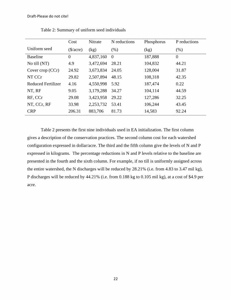
Table 2 presents the first nine individuals used in EA initialization. The first column

gives a description of the conservation practices. The second column cost for each watershed

configuration expressed in dollar/acre. The third and the fifth column give the levels of N and P

expressed in kilograms. The percentage reductions in N and P levels relative to the baseline are

presented in the fourth and the sixth column. For example, if no till is uniformly assigned across

the entire watershed, the N discharges will be reduced by 28.21% (i.e. from 4.83 to 3.47 mil kg),

P discharges will be reduced by 44.21% (i.e. from 0.188 kg to 0.105 mil kg), at a cost of $4.9 per

acre.


23

The ambient level associated with each individual (watershed configuration) is evaluated

by watershed water quality model, SWAT. The total cost is obtained by evaluating each

individual at the set of conservation practices costs. Thus, each individual, watershed

configuration, has associated a cost and a particular level of nitrogen and phosphorus.

Using the above information (cost, N and P data), EA compares each individual with all

other individuals. Following all possible comparisons, an individual is Pareto dominant if it has

either both levels of nitrogen and phosphorus lower at the same level of cost, or, alternatively, at

the same level of reductions it has a lower cost. After all individuals have been compared, each a

strength value is assigned to each individual. The strength value of a particular individual counts

how many individuals dominate it (how many individuals have lower costs, or given the same

costs have a higher level of reduction). A measure of fitness is computed, providing the selection

or survival criterion. A lower value for the fitness score gives a higher the probability of an

individual to be selected for next generation. The Pareto frontier is constructed by individuals

with a fitness score equal to zero, i.e.; they are not dominated by any other individuals. A density

measure is useful later on, to avoid the clustering effect and allow the Pareto frontier to span over

a larger area of the search space.

The Pareto dominant individuals are selected to be the next generations’ parents. New

offspring emerge as a result of the crossover and mutation processes. Once a new population is

created, the process described above is repeated. This algorithm can be run over any number of

generations. Once the algorithm is stopped, the solution, a frontier, consists of a set of non

dominated individuals. In the context of watershed scale analysis, the individuals represent

different watershed configurations. In particular, one individual represents optimal placement of

a set of conservation practices that achieves a particular level of nitrogen and phosphorus in the

least costly way.

To check the algorithm sensitivity given that the number of generations allowed to

survive is increased, the algorithm was run in steps. In particular, a Pareto frontier was saved

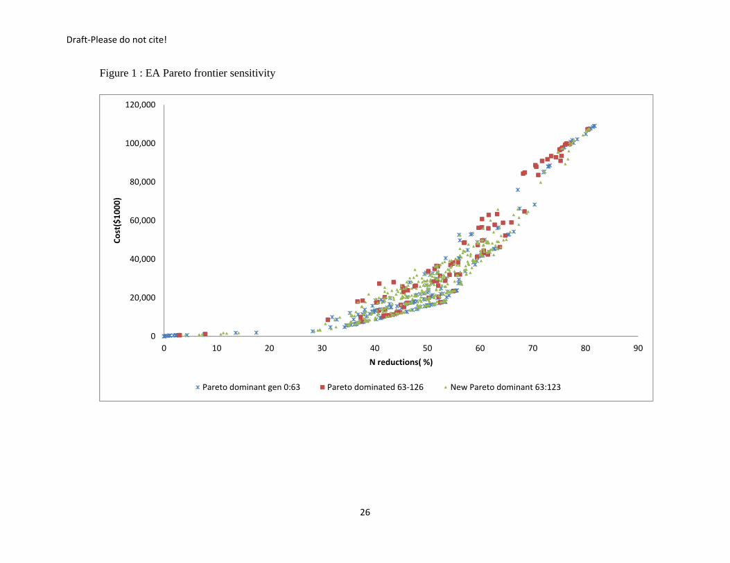
after every 63 generations and another one after another 60 generations. Figure1 depicts the

evolution of Pareto frontiers in terms of nitrogen (N) percentage reductions on the X- axis and

associated costs expressed in as thousand dollars on the Y-axis. The frontiers should move

downright, meaning that as more generations are allowed, better solutions are found. Also, the


24

individuals that are on the first frontier and survive the first 63 generations but do not survive the

next 60 generations, being dominated, should lie on the inner side of the frontier created after the

first 63 generations.

Figure1 depicts the changes in EA’s frontier when the number of generations is increased

from 63 to 123. The blue stars represent the Pareto dominant individuals that survive at the end

of 63 generations. The red squares represent the individuals that survive the first 63 generations,

but are dominated after another 60 generation. Note their position is on the inner part of the

frontier. Finally, the green triangles represent the new dominant individuals, individuals that

where created between generation 63 to 123. Notice that their locations on the frontier is farther

on the downright part of reduction – cost space, meaning that EA found either individuals that

achieve the same level of reduction less costly, either individuals that achieve higher levels of

reduction at the same cost.

4 Cost asymmetry: Cost saving empirical assessment

The regulator uses the SWAT-EA analysis to find the optimal placement of abatement

practices given his assumption about costs, . The result, a Pareto frontier, consists of hundreds

of individuals, or watershed configurations, able to achieve different combinations of nitrogen

(N) and phosphorus (P) reductions in the least cost way. Once the frontier is generated, the

authority is able to choose the ambient pollution target. Furthermore, for each field he can assign

the optimal conservation placement and optimal amount of discharges measured either at the

edge-of –field, either at the watershed exit.

The true costs, , associated with this set of practices may differ from the costs that the

authority uses. If a tradable performance standard program is implemented, each farm will

minimize its abatement effort by choosing from the same set of conservation practices such that

the edge-of-field emissions are less than the standard imposed by the environmental authority.

The individual standards are designed such that the ambient cap is binding at the main watershed

outlet.

Two different sets of EA optimization are performed in order to show the cost difference

due asymmetric information. The first EA optimization uses a set of costs determined by using


25

real field data, where a conservation practice has the same the per acre estimate for each farm or

field. The EA optimizations allowed 180 generations to survive. The Pareto frontier consists of

more than 1,014 individuals. The first EA optimization is corresponding to environmental

agency cost minimization problem with the conservation costs expressed in mean levels (i.e. cost


26

Figure 1 : EA Pareto frontier sensitivity

0

20,000

40,000

60,000

80,000

100,000

120,000

0 10 20 30 40 50 60 70 80 90

Cost($10

00)

N reductions( %)

Pareto dominant gen 0:63 Pareto dominated 63‐126 New Pareto dominant 63:123


27

minimization defined by equation (2.15). The total cost is equivalent to equation (2.16). It

represents the least cost of achieving a particular combination of N and P discharges.

∑ , (2.21)

The set of individuals on this frontier will be referred as :

| ∧ ; ∀ 1, … ,1014 (2.22)

Equation (2.22) defines as the set of all solutions generated by EA optimization;

where each element of the set gives the least cost solution for achieving a unique combination of

and discharges.

The second EA optimization corresponds to the individual cost minimization problem or

the outcome of a tradable performance standard program defined by equation (2.17). It uses the

same set of conservation practices as first EA optimization, but incorporates the asymmetric

information aspect of the problem, by allowing the cover crops to vary across watershed. Total

cost is equivalent to equation (2.18):

∑ , (2.23)

The second Pareto frontier consists of 914 individuals; the solutions set will be referred

as , and can be defined in a similar way to

| ∧ ; ; ∀ 1,… ,914 (2.24)

Equation (2.24) defines as the set of all solutions generated by EA optimization;

where each element of the set gives the least cost solution for achieving a unique combination of

and discharges.

The and are different frontiers generated with two different cost sets. Given

the different nature of the two sets, solutions must be transformed in terms of :

.Pareto frontier is re-evaluated with the set of conservation costs used to obtain

frontier. The new frontier is referred as .

∈ | ∑ , ∀ 1,… ,1014 (2.25)


28

If there any cost savings, then for the same level of ambient target, the cost associated

with an individual from frontier should be higher than an individual on frontier.

The cost comparison is made as it follows. First, each individual in was reevaluated at

the true set of costs, , obtaining . This could be easily done, since the SWAT_EA

output provides the placement of conservation practices and area data is available is available for

each field. After this transformation, individuals from and can be compared. The

cost comparison is made by selecting individuals from the two sets that achieve the same, or

almost the same ambient levels in N (nitrogen) and P (phosphorus). The set of individuals

subject to cost comparison, , is given by:

∩ ; where

∩ ∈ ∧ ∈ | ≅ ∧

≅ ( 2.26)

versus

Before presenting the outcome of the above comparison, it would be interesting to take a

look at the difference between and . This is to determine how much a command

and control cost if the true costs are given by . A priori, we have no beliefs about the size and

the direction of the differences. The is the EA solutions where a single cost for cover

crops is used; solution reevaluates the former solution by using a set cost of six

estimates for cover crops. and compare the same individuals but evaluated at

different set of costs.

Table 3 summarizes the comparison results. First column shows the percentage reduction

levels in terms of nitrogen. The second column gives the distribution of the individuals

that are less expensive than corresponding individuals. The third column presents by

how much, on average, the costs are underestimated. The fourth and the fifth columns are the

mirror cases for the second and the third columns and represent the cases of the individuals that

are more expensive. There are 319 individuals whose costs were underestimated. Among these

254 have N percentage reductions between 40 % and 60 %. The cost of each individual was, on

average, underestimated by 1.35 %. On the other side, there are 695 individuals whose costs


29

would be overestimated. Among these, 546 individuals have both N and P percentage reductions

between 40 % and 60 %, and the costs being overestimated by 1.1%.

Table 3: vs

N reductions

(%)

<

% Cost

underestimation

>

% Cost

overestimation

less than 40 52 1.65 65 1.13

between 40-60 254 1.35 546 1.1

more than 60 12 0.2 84 0.96

Total Individuals 319 695

This comparison exercise is useful to show that, in the case of a command and control

program, for some levels of pollution reductions, the regulator's beliefs about the overall cost

program are be overestimated, but for the most of the cases, the overall cost are underestimated.

Even if the deviations are small, around one percent, it should keep in mind, that only cover

crops cost was varied.

. versus

The following costs comparisons are based on and solution sets. is

the result of EA optimization that used a single cost estimate for each conservation practices. The

purpose of is to make the ‘‘authority” optimization solution comparable with farm

level optimization solution. If in the case the individuals subject to

comparison were on the same (i.e. located on the same frontier), in this case the compared

individual lie on two different Pareto frontiers. In order to make the comparison as accurate as

possible, the selected individuals have similar levels of N and P reductions ( i.e. within an

interval of 0.01 percent ).

Before comparing the chosen individuals, it is useful to have an overall picture of how all

individuals that define set stands relative to individuals on set. Figure 2 depicts


30

the percentage reductions in N, on the horizontal axis, versus cost, expressed in $1000, on

vertical axis. The blue triangles represent the set, and the green stars represent

set. If there are any cost gains, the curve should bend more outward (achieve higher level

of reduction at the same costs, or achieve the same level of reductions at lower costs). The

results, at this stage, are ambiguous, with some areas where is lower than curve,

with some other areas that do not support the cost savings. This might be due to several factors.

First, graph takes into account only N reductions and disregard P reductions. Second, due to the

approximation natures of EA algorithm, there are only a few exact matches with respect both N

and P reductions. For example, some individuals on set are characterized 40.35%

reductions in N and 51.25% reductions in P, but a corresponding individual on curve

at the same level of N reductions has different levels of P reduction.

Next, we describe the individuals chosen for comparison. The individuals were chosen

according to equation (2.26). Seven pairs of individuals were selected from each set sets by

requiring the same N reductions while as the absolute difference in P reductions within 0.001.

The selected pairs are presented in Table 4. The first and the fourth columns indicate the

individual’s position in its set. The numbers itself do not bear a great importance but provide

information about timing, i.e. whether they were “born” later or sooner in the EA’s evolution. A

higher position number means that the individual was created after a higher number of

generations. The second and the third columns present N and P percent reductions associated

with the individuals that were selected from set. The fifth and the sixth column offer

similar information regarding the individuals form set. The seventh column introduces the

absolute size of the cost savings; finally the last column represents the cost savings as

percentage.


31

Table. 4. Individuals versus Individuals

# #

N % P % N % P % Cost %

1 0 0 1 0 0 0 0

4 28.21 44.21 4 28.21 44.21 0 0

6 34.27 44.59 6 34.27 44.59 0 0

9 81.73 92.24 9 81.73 92.24 0 0

303 42.64 44.63 1450 42.64 44.64 81,375.3 0.77

940 28.22 44.19 1657 28.22 44.19 - -0.13

1892 51.26 56.03 2042 51.26 56.03 173,074. 0.59

The first four pairs are identical and have zero cost savings; i.e. the individuals achieve

the same target with the same cost. The position numbers indicate that these individuals coincide

with the initial individuals where a single practice is used. The first pair represents the baseline

scenario, the second pair represents no till only scenario, the third pair represents the scenarios

where reduced fertilizer is used in conjunction with no till, and finally , the last pair represents

the scenario were all land is retired out of production. The results are as expected since, there is

no change in costs for these conservation practices. The pairs (#303 ,#1450) and (#1892, #2042)

have higher than (i.e. the idea of cost savings is supported). One pair of

individuals (#940,#1657) has negative savings.

Table 5 describes the distribution of conservation practices as percentage of total area in

the watershed. Table 6 describes the field frequency for each conservation practice (how many

fields use a particular conservation practice) .The most used practices are combinations of

reduced fertilizer and no till (CS6), or reduced fertilizer, no till and cover crops(CS8).


32

Figure 2 –

0

20000

40000

60000

80000

100000

120000

0 10 20 30 40 50 60 70 80 90

Cost ($

1000

)

N reductions (%)

CACPSsol PSsol


33

Table 5 Distribution of conservation practice by area : % in total watershed area13

CS1 CS2 CS3 CS4 CS5 CS6 CS7 CS8 CS9

940 0 100 0 0 0 0 0 0 0

303 0 0 0 11 0 58 0 30 0

1892 1 0 0 16 0 40 0 24 19


1657 0 100 0 0 0 0 0 0 0

1450 0 0 0 0 0 60 0 39 0

2042 0 0 0 7 0 43 0 31 19

Table 6 Distribution of conservation practice: field frequency


940 3 2874 2 22 0 0 0 1 0

303 5 1 3 443 4 1606 5 830 5

1892 7 8 5 504 6 1139 7 695 531


1657 3 2874 2 0 0 0 0 23 0

1450 6 9 9 6 5 1687 8 1172 0

2042 7 8 8 175 2 1256 8 833 609

13 CS1: baseline; CS2: no till; CS3: cover crops; CS4 no till and cover crops; CS5; Reduced fertilizer; CS6 reduced fertilizer and no till, CS7 reduced fertilizer and cover crops; CS8: reduced fertilizer, cover crops and no till, CS9 land retirement;


34

The individuals of the first pair (#940, #1657) have almost the same placement for

conservation practice The only difference is given by the #22 individual that switches

from no till and cover crop ( CS4) to cover crops, no till and reduced fertilizer (CS8), the 22

The negative value could be explained as an approximation error.

The next two pairs have cost savings. The pair ( #303, #1450) has the highest relative

cost savings. Individual #303 has 11 % of its area in no till and cover crop (CS4), 58% percent in

reduced fertilizer and no till (CS6) , and the rest in no till, reduced fertilizer and cover crops

(CS8). Under , the #1450 individual’s configuration does not include no till and cover crops

(CS4), instead area covered by reduced fertilizer and no till (CS6) increased by 1 % and area

covered by reduced fertilizer, no till and CRP (CS8) increased by 10 %.

The last pair (#1892, #2042) has the highest absolute cost savings. Individual #1892

places 40% of its area in no till and cover crops (CS8), 24 % in reduced fertilizer, no till and

cover crops (CS9), and finally 19% in CRP (CS9). Individual #2042 under has a similar

watershed configuration places 7% of its area in no till and cover crops (CS4), 43 % in reduced

fertilizer and no till (CS6), 31% in reduced fertilizer, no till and cover crops (CS8), the

difference is in CRP (CS9).

5 .Conclusions

In the setup considered here, the regulator seeks to enforce a cap on total ambient

pollution. Two alternatives are investigated: a command and control program and a tradable

performance based standard program. In the first one, the authority, using an incomplete cost

information set, decides what conservation practices to be implemented by each farm. In the

second case, the authority recognizes that it does not have complete cost information and

implements a performance standard program, allowing farmers to choose the conservation

practice according to their cost information.

Two different SWAT_EA optimizations are performed to generate the results needed to

confirm or infirm the cost savings. First optimization uses a unique set of conservation costs, .

The Pareto frontier represents the solutions of a command and control program. Second

optimization is equivalent to individual optimization problem under a tradable performance


35

standard program. The costs set used in the second optimization reflects the cost heterogeneity

across the watershed by imposing variation for the cost of cover crops, .

Overall, the size of the costs savings under a tradable performance standard program is

small, but it should be kept in mind only one conservation cost had been diversified across

watershed. Further analysis must be conducted where the cost of each conservation practice is

varied across the watershed’s fields.


36

References:

Arnold, J.G., Srinivasan,R., Mutiahh, R.S., and Williams, J.R.,, 1998, “Large area hydrologic

modeling and assessment part I: Model development”, Journal of American Water

Resources Association 34 (1) :73:89

Arnold, J.G., and Fohrer, N. 2005. Current capabilities and research opportunities in applied

watershed modeling. Hydrological Processes 19: 563-572.

Bekele, E.G and Wicklow,J.W, 2005.” Multiobjective management of ecosystem services by

integrative watershed modeling and assessment part I: Model development” Water

Resources Research, 41, W10406, doi:10.1029/2005WR00590

Carpentier,C.L.,Bosch,D.J. ans Batie,S.1998 “Using spatial information to reduce costs of

controlling agricultural nonpoint source pollution”. American Journal of Agricultural

Economics, 61:401-413

Coase, R.H. 1960 The problem of social cost. J Law Econ 3(1):1–44

Colby, B.G (1990) Transactions costs and efficiency in western water allocation, Am. J. Agric.

Econ. 72 ,pp. 1184–1192

Crocker, T. 1966. “The structuring of atmospheric pollution control systems, volume 1 of the

economics of air pollution”. Journal of Economic Theory, 5(3): pp. 395-418.

Corn N rate calculator. Iowa State University Agronomy Extension. Available at

http://extension.agron.iastate.edu/soilfertility/nrate.aspx. Accessed April 2010. File C2-

10

Dales ,J.H. 1968 Land, water and ownership. Can J Econ 1(4):791–804

Edwards, W, and D. Smith.2009 Cash rental rates for Iowa 2009 survey. Iowa State University

Extension Ag. Decision Maker

Feng and C. Kling 2005 The consequences of cobenefits for the efficient design of carbon

sequestration programs, Canadian Journal of Agricultural Economics 53 (2005), pp.


37

Hongli Feng, Manoj Jha, and Phil Gassman 2009 The Allocation of Nutrient Load Reduction

across a Watershed: Assessing Delivery Coefficients as an Implementation Tool Appl.

Econ. Perspect. Pol. 31: 183-204. 461–476.

Gassman, P.W., M. Reyes, C.H. Green, and J.G. Arnold. 2007. “The Soil and Water

Assessment Tool: Historical development, applications, and future directions”. Trans.

ASABE. 50(4):1211-1250.

Gassman, P.W. 2008. A Simulation Assessment of the Boone River Watershed: Baseline

Calibration/Validation Results and Issues, and Future Research Needs. Ph.D.

Dissertation, Iowa State University, Ames, Iowa.

Gitau, M.W., T. L. Veith, andW. J. Gburek (2004), “Farm-level optimization of BMP

placement for cost-effective pollution reduction” , Trans. ASAE, 47(6), 1923–1931.

Hung, M. and D. Shaw, 2004. A Trading-Ratio System for Trading Water Pollution Discharge

Permits. Journal of Environmental Economics and Management 49:83–102.

Khanna, M.,W.H. Yang, and R. Farnsworth.2003. “Cost-effective Targeting of Land

Retirement to Improve Water Quality with Endogenous Sediment Deposition

Coefficient”, American Journal of Agricultural Economics, 85(3), pp. 538-53.

Krupnick A, Oates W,VergEVD .1983. “On marketable air pollution permits: the case for a

system of pollution offset.” J Environ Econ Manage 10:233–247

Kling ,C.L., S. Secchi, M. Jha, L. Kling , H. Hennessy, and P.W. Gassman 2005. “Non point

source needs assessment for Iowa : The cost of improving Iowa’s water quality. Final

Report to the Iowa Department of Natural Resources. Center for Agricultural and Rural

Development, Iowa State University, Ames, Iowa

Kurkalova, L.A., C. Burkart, and S. Secchi. 2004. “Cropland Cash Rental Rates in the Upper

Mississippi River Basin.” CARD Technical Report 04-TR 47. Center for Agricultural and

Rural Development, Iowa State University.

Mitchell,M., 1996 An introduction to genetic algorithms. Cambridge, Massachusetts; MIT press


38

Libra, R.D, Wolter, Langel, C.F., 2004. Nitrogen and phosphorus budget for Iowa and Iowa

watersheds. Iowa Geological Survey, Technical Information Series 47.

Maringanti,C., Chaubey, I., Popp, J. 2009 “Development of a multiobjective optimization tool

for the selection and placement of best management practices for nonpoint source

pollution control” Water Resources Research

Montgomery, W.D .1972 “Markets in licenses and efficient pollution control programs”. J.

Econ. Theory (3):395–418

Morgan, C.L., Coggins, J.S., Eidman, V.R. 2000 “Tradable permits for controlling nitrates in

groundwater at the farm level: a conceptual model” . J Agric Appl Econ 32(2):249–258

Prabodanie, R.A.R, Raffensperger, J.F,nd Milke, M.V .2010 “A Pollution Offset System for

Trading Non-Point Source Water Pollution Permits”, Environmental and Resource

Economics 45(4)499-515

Rabotyagov, S. 2007"Four Essays on Environmental Policy under Uncertainty with

Applications to Water Quality and Carbon Sequestration." Ph.D. thesis, Department of

Economics, Iowa State University

Sawyer, J., E. Nafziger, G. Randall, L. Bundy, G. Rehm, B. Joern. 2006. Concepts and rational

for regional nitrogen rate guidelines for corn. Iowa State University, Ames, Iowa.

Available at: http://extension.agron.iastate.edu/soilfertility/nrate.aspx.

Secchi, S., B.A. Babcock “Impact of High Crop Prices on Environmental Quality: A Case of

Iowa and the Conservation Reserve Program” 2007,Working Paper 07-WP 447. Center

for Agricultural and Rural Development Iowa State University,Ames, Iowa

Secchi, S., P. Gassman, M. Jha, H.H. Feng, T. Campbell, and C. Kling. 2007 “The Cost of

cleaner water: Assessing agricultural pollution reduction at the watershed scale. Journal

of Soil and Water Conservations 62 (1):10:21

Shortle, J. S., D. G. Abler. 1997 “Nonpoint pollution”, in H. Folmer and T. Tietenberg, eds.,

The International Yearbook of Environmental and Resource Economics. Cheltenham,UK

Eduard Elgar.


39

Srivastava, P, Hamlett, J.M., Robillard, P.D, Day, R.L, 2002, “Watershed optimization of best

management practices using AnnAGNPS and a genetic algorithms”, Water and resources

Research, 38(3): 1-14;

US EPA 2003. Water Quality Trading Policy, Office of Water, January 13.

(http://www.epa.gov/owow/watershed/trading/tradingpolicy.html).

US EPA, 2004. Water Quality Trading Assessment Handbook: Can Water Quality Trading

Advance Your Watershed’s Goals?

(http://www.epa.gov/owow/watershed/trading/handbook/ )

Vache, K.B, Eilers,J.M. and Santelman,M.V .2002. “Water quality of alternative agricultural

scenarios in the U.S corn belt”. Journal of the American Water Resources Association,

38(2):773-787

Veith, T.L, Wolfe,M.L and Heatwole, C.D. 2003, “Development of optimization procedure for

cost effective BMP placement”. Journal of American Water Resources Association,

39(6):1331:1343

Zitzler, E., and L. Thiele (1999), “Multiobjective evolutionary algorithms: A comparative case

study and the strength Pareto approach”, IEEE Trans. Evol. Comput., 3(4), 257– 271;


40

a pollution trading system with cost assymetryageconsearch.umn.edu/bitstream/103719/2/a pollution...

Documents