a pilot study for several pumping stations in the ... · pompstations zijn gelegen in het centrale...
TRANSCRIPT
RIVM report 703717011/2003
Determination of denitrification parameters indeep groundwater
A pilot study for several pumping stations in theNetherlands
G.J.M. Uffink
This research has been carried out by order of the Directoraat-Generaal voor Milieubeheer,Directie Bodem, Water en Landelijk gebied, as part of project 703717.
RIVM, P.O. Box 1, 3720 BA Bilthoven, telephone: 030 - 274 91 11; fax: 030 - 274 29 71

Page 2 of 76 RIVM report 703717011

RIVM report 703717011 Page 3 of 76
Abstract
Groundwater nitrate measurements in the central and eastern parts of the Netherlands showedthat denitrification occurs in many locations. This is why models used for analysis ofmanagement decisions for drinking-water production need to take denitrification into account.Little information is available on the denitrification rate and its spatial distribution. In thisreport a model concept is proposed to simulate denitrification and a pilot study is carried outfor nine groundwater pumping stations in the central and eastern part of the Netherlands. Theunknown parameters were determined using a calibration procedure with the optimisationprogram PEST. Nitrate measurements from monitoring networks were used for thecalibration, along with nitrate data from the water abstracted at a number of public drinking-water pumping stations. In zones where the presence of organic substances is likely,denitrification is described as an exponential decay with a half-life of about 500 days. Inzones where organic material is absent, the half-life is much higher (2750 days).Instantaneous nitrate reduction is assumed at or near the phreatic surface. Here, an averagereduction of 50% is found. However, this figure may also represent a compensation for anover- or underestimation of the nitrate input at the water table. The parameter values werefound to contain a large measure of uncertainty, for which several explanations are suggestedand discussed. One factor that affects the parameter uncertainty is related to thesimplifications in the model set-up. A second source of ‘uncertainty’ is due to parameters inthe model that provided input data, such as groundwater velocities (LGM) and nitrate fluxes(STONE). Finally, a certain amount of uncertainty is inherent in the stochastic technique usedfor the solute transport simulation (Random Walk technique).

Page 4 of 76 RIVM report 703717011
RIVM report 703717011 Page 5 of 76
Contents
Samenvatting 7
1. Problem description 11
2. Former investigations 13
3. Study area 153.1 General 153.2 Surface waters 183.3 Aquifer system 193.4 Groundwater heads and velocities 22
4. Groundwater abstraction 274.1 Rates of discharge 274.1 Locations 28
5. Data and models 315.1 Nitrate measurements 315.2 Leachate model 315.3 Groundwater model 325.4 Solute transport model 34
6. Denitrification 376.1 General 376.2 Implementation 38
7. Calibration 457.1 Parameters 457.2 Log transform of concentrations 457.3 Software 467.4 Procedure 47
8. Results 498.1 Calibration results 498.2 Uncertainty 55

Page 6 of 76 RIVM report 703717011
8.3 Spatial distribution 578.4 Match of observed and calculated breakthrough curves 58
9. Summary and conclusions 65
Acknowledgements 69
References 71
Mailing List 75
RIVM report 703717011 Page 7 of 76
Samenvatting
Bij de modellering van nitraattransport in grondwater moet men zowel in ondiepe als in diepeaquifers rekening houden met denitrificatie (Kovar et al., 1998, RIVM rapport 730717002). Indit rapport wordt voor het denitrificatieproces een modelconcept voorgesteld dat bestaat uitdrie afzonderlijke processen die zich met verschillende snelheid manifesteren:i) een instantane nitraatreductie die zich afspeelt aan of in de buurt van het freatisch vlak;ii) een betrekkelijk snel verlopend exponentieel verval dat optreedt in een zone waar zich
voldoende organisch materiaal bevindt;iii) een betrekkelijk langzaam verlopend exponentieel verval in de zone waar organisch
materiaal nagenoeg afwezig is.Om de parameters van de hierboven genoemde processen te bepalen, is in deze pilotstudy eenkalibratie-procedure opgezet. Voor de eigenlijke kalibratie is het model onafhankelijkeoptimalisatieprogramma PEST gebruikt. Gedurende het kalibratie-proces wordenmodeluitkomsten vergeleken met meetgegevens. Als meetgegevens zijn nitraatmetingengebruikt van waarnemingsputten die behoren tot het Landelijk en/of Provinciaal MeetnetGrondwater, (LMG en/of PMG). Daarnaast zijn nitraatmetingen gebruikt van het water dat opverschillende grondwaterwinplaatsen voor de openbare drinkwatervoorziening wordtgewonnen en als reinwater wordt afgeleverd, veelal na zuivering. De negen geselecteerdepompstations zijn gelegen in het centrale en oostelijke deel van Nederland, waar goeddoorlatende freatische watervoerende pakketten voorkomen. Nitraatmetingen inwaarnemingsputten kunnen worden beschouwd als puntwaarnemingen, zowel ruimtelijk als inde tijd. Zij vertegenwoordigen slechts een klein ruimtelijk gebied en een korte tijdsperiode.De gegevens van het in de pompstations onttrokken water zijn representatief voor een veelgroter gebied. In horizontale zin komt dat gebied overeen met het intrekgebied van hetpompstation. Nitraatgegevens van het onttrokken water en het afgeleverde drinkwater wordensinds 1992 verzameld in het kader van het REWAB meetprogramma (REgistratie opgavenvan WAterleidingBedrijven). Van voor 1992 zijn metingen beschikbaar van het LandelijkMeetnet Drinkwaterkwaliteit (LMD). De LMD metingen hebben alleen betrekking op hetwater na de zuiveringsstap (te weten reinwater metingen). In geen van de pompstations wordtoverigens een specifieke nitraatzuivering toegepast. In een aantal gevallen zijn denitraatgehalten voor en na de zuiveringsbehandeling vrijwel identiek. In andere gevallen(bijvoorbeeld bij Pompstation Herikerberg) is dat echter niet het geval.
Modellering van nitraattransport is niet mogelijk zonder informatie over de hoeveelheid nitraatdie aan het freatisch oppervlak het grondwatersysteem binnen gaat. De daadwerkelijkewaarden voor deze nitraatflux zijn niet beschikbaar op de schaal van in dit rapport gebruiktemodel. In deze studie worden waarden gebruikt die zijn gegenereerd met het uitspoelingsmodelSTONE. Het modelconcept van STONE wijkt echter sterk af van dat van het grondwater

Page 8 of 76 RIVM report 703717011
model, zowel in ruimtelijke als temporele zin. Verschillende vereenvoudigingen warennoodzakelijk om de STONE-gegevens om te werken naar het ‘format’ dat was gewenst voorhet grondwatertransportmodel. Een andere vereenvoudiging betreft hetgrondwaterstromingsmodel zelf. De grondwaterstroming is hier opgevat als een stationairprobleem. Het is echter bekend dat met name de onttrekkingshoeveelheden van depompstations gedurende de gesimuleerde periode (1950-2000) niet constant is geweest. Deaangebrachte vereenvoudigingen waren noodzakelijk om het rekenwerk mogelijk te maken,maar zij bemoeilijken wel de uiteindelijke vergelijking van modelresultaten met dewaarnemingen.
Voor de ‘instantane’ denitrificatie nabij het freatisch oppervlak is een gemiddelde reductiefactor gevonden van 47%. Deze factor wordt echter sterk beïnvloed door onzekerheden in dedoor STONE gegenereerde nitraat-input. Voor droge zandgronden zijn deze waarden eenfactor van 30% te hoog (Overbeek et al, 2001b). De gevonden denitrificatie-factor kan,onbedoeld, tevens dienst doen als een compensatie voor mogelijke overschattingen van denitraatinput. Het is niet mogelijk om het aandeel van een daadwerkelijke denitrificatie en datvan het compensatie-effect nader te preciseren. De gevonden parameters voor de exponentieelverlopende denitrificatie worden in dit rapport uitgedrukt als halfwaardetijden. Voor de zonewaar organische materiaal aanwezig wordt verondersteld – dwz onder beek- en rivierdalen enin de omgeving van kleilagen – is een gemiddelde halfwaardetijd gevonden van ongeveer 500dagen, variërend van 165 tot 1485 dagen. Uffink en Römkens (2001) vonden hier eensoortgelijke waarde ( 1
21 jaar). Voor de zone met langzaam exponentieel verval is eenhalfwaardetijd van rond 2750 dagen gevonden, variërend van 1680 tot 4450 dagen. Dezewaarden liggen hoger dan die uit de rapportage van Uffink en Römkens (3 tot 5 jaar). Dezelaatste studie had betrekking op een klein deelgebied van het studiegebied dat in het huidigerapport wordt beschouwd, terwijl een handmatige kalibratie werd toegepast en uitsluitendnitraatmetingen werden gebruikt van de meetnetputten.
De onzekerheid van de gevonden parameters is tamelijk groot. Dit is het gevolg van een aantalfactoren. Allereerst zijn er verschillende vereenvoudigingen in de model-opzet aangebracht.Omdat de grondwaterstroming stationair wordt verondersteld en de nitraatinvoer is omgewerktnaar langjarige gemiddelden, zullen seizoensschommelingen in de modeluitkomsten nietzichtbaar zijn. In de ondiepe waarnemingsputten zijn seizoensvariaties wel aanwezig. Ook degeleidelijke toename van de door de pompstations onttrokken hoeveelheid water wordt in hetmodel niet in rekening gebracht. Een tweede belangrijke bron van onzekerheid loopt via demodellen die invoergegevens leveren voor de transportsimulatie, zoals degrondwatersnelheden (LGM) en de nitraatfluxen (STONE). Aangezien onzekerheden van dezegegevens niet bij de kalibratie zijn betrokken, komen deze uiteindelijk terecht bij de geschattetransportparameters. Tenslotte bestaat er een vorm van onzekerheid die inherent is aan degebruikte oplossingstechniek in het transportmodel. De stochastische component in de‘particle-tracking’ methode veroorzaakt een ‘ruis’ die alleen kan volledig worden geëlimineerd
RIVM report 703717011 Page 9 of 76
door een oneindig aantal deeltjes toe te passen. In praktijk zal daarom altijd een zekere matevan ruis in de modelresultaten worden geaccepteerd. Een meer algemeen probleem dateveneens met het bovenstaande te maken heeft, is het volgende. Bij lange-termijnvoorspellingen en beleidsanalyses op regionale schaal worden meestal sterk opgeschaaldemodellen gebruikt. In het algemeen zijn voor kalibratie van deze modellen alleen gegevensbeschikbaar die afkomstig zijn van kleinschalige en kort lopende processen. Dezeinconsistentie tussen de schaal van de waarnemingen en de resolutie van demodelberekeningen staat een zinvolle vergelijking tussen modelresultaten en waarnemingenvaak in de weg. Zolang middelen of technieken om de parameteronzekerheid te reduceren nietvoorhanden zijn, lijkt een landsdekkende toepassing van de beschreven kalibratieprocedurenog niet zinvol.
Kalibratie leidt niet altijd tot een unieke verzameling parameterwaarden. Moeilijkheden bij dit‘niet uniek zijn’ kunnen worden opgelost door een stapsgewijze kalibratie-procedure. Bijiedere afzonderlijke stap laat men slechts één of enkele parameters variëren, waarbij slechts demeetgegevens worden geselecteerd die het meest gevoelig zijn voor de vrije parameter(s). Deselectie van de meest gevoelige waarnemingen kan het best gebeuren aan de hand van eengevoeligheidsanalyse. Dit is echter met de hier gebruikte versie van PEST niet mogelijk. Bijtoekomstige kalibratieberekeningen wordt een gevoeligheidsanalyse echter sterk aanbevolen.

Page 10 of 76 RIVM report 703717011
RIVM report 703717011 Page 11 of 76
1 Problem description
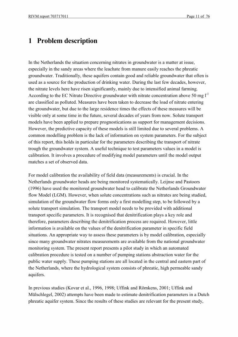
In the Netherlands the situation concerning nitrates in groundwater is a matter at issue,especially in the sandy areas where the leachate from manure easily reaches the phreaticgroundwater. Traditionally, these aquifers contain good and reliable groundwater that often isused as a source for the production of drinking water. During the last few decades, however,the nitrate levels here have risen significantly, mainly due to intensified animal farming.According to the EC Nitrate Directive groundwater with nitrate concentration above 50 mg l-1
are classified as polluted. Measures have been taken to decrease the load of nitrate enteringthe groundwater, but due to the large residence times the effects of these measures will bevisible only at some time in the future, several decades of years from now. Solute transportmodels have been applied to prepare prognostications as support for management decisions.However, the predictive capacity of these models is still limited due to several problems. Acommon modelling problem is the lack of information on system parameters. For the subjectof this report, this holds in particular for the parameters describing the transport of nitratetrough the groundwater system. A useful technique to test parameters values in a model iscalibration. It involves a procedure of modifying model parameters until the model outputmatches a set of observed data.
For model calibration the availability of field data (measurements) is crucial. In theNetherlands groundwater heads are being monitored systematically. Leijnse and Pastoors(1996) have used the monitored groundwater head to calibrate the Netherlands Groundwaterflow Model (LGM). However, when solute concentrations such as nitrates are being studied,simulation of the groundwater flow forms only a first modelling step, to be followed by asolute transport simulation. The transport model needs to be provided with additionaltransport specific parameters. It is recognised that denitrification plays a key role andtherefore, parameters describing the denitrification process are required. However, littleinformation is available on the values of the denitrification parameter in specific fieldsituations. An appropriate way to assess these parameters is by model calibration, especiallysince many groundwater nitrates measurements are available from the national groundwatermonitoring system. The present report presents a pilot study in which an automatedcalibration procedure is tested on a number of pumping stations abstraction water for thepublic water supply. These pumping stations are all located in the central and eastern part ofthe Netherlands, where the hydrological system consists of phreatic, high permeable sandyaquifers.
In previous studies (Kovar et al., 1996, 1998; Uffink and Römkens, 2001; Uffink andMülschlegel, 2002) attempts have been made to estimate denitrification parameters in a Dutchphreatic aquifer system. Since the results of these studies are relevant for the present study,

Page 12 of 76 RIVM report 703717011
the report starts with an overview of this work (Chapter 2). In Chapter 3 some topographicaland geohydrological features of the present model area are described, while Chapter 4 givesinformation with respect to the groundwater abstraction sites in the area. The data and modelsthat have been used in this study are briefly described in Chapter 5. Since denitrification is themain point of interest in the present study, a separate chapter is devoted denitrification. It alsospecifies the implementation of this process in the transport module. The calibrationprocedure itself is described in more detail in Chapter 7. Finally, the calibration results arepresented and discussed in Chapter 8.
RIVM report 703717011 Page 13 of 76
2 Former investigations
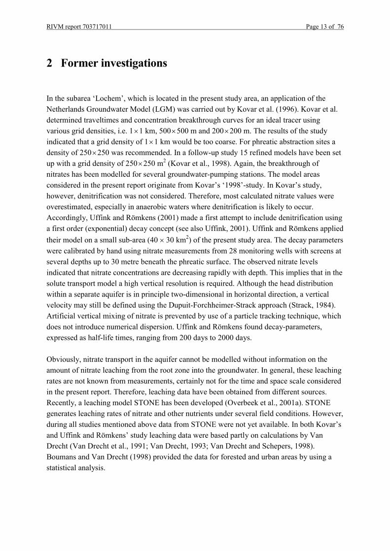
In the subarea ‘Lochem’, which is located in the present study area, an application of theNetherlands Groundwater Model (LGM) was carried out by Kovar et al. (1996). Kovar et al.determined traveltimes and concentration breakthrough curves for an ideal tracer usingvarious grid densities, i.e. 1�1 km, 500�500 m and 200�200 m. The results of the studyindicated that a grid density of 1�1 km would be too coarse. For phreatic abstraction sites adensity of 250�250 was recommended. In a follow-up study 15 refined models have been setup with a grid density of 250�250 m2 (Kovar et al., 1998). Again, the breakthrough ofnitrates has been modelled for several groundwater-pumping stations. The model areasconsidered in the present report originate from Kovar’s ‘1998’-study. In Kovar’s study,however, denitrification was not considered. Therefore, most calculated nitrate values wereoverestimated, especially in anaerobic waters where denitrification is likely to occur.Accordingly, Uffink and Römkens (2001) made a first attempt to include denitrification usinga first order (exponential) decay concept (see also Uffink, 2001). Uffink and Römkens appliedtheir model on a small sub-area (40 � 30 km2) of the present study area. The decay parameterswere calibrated by hand using nitrate measurements from 28 monitoring wells with screens atseveral depths up to 30 metre beneath the phreatic surface. The observed nitrate levelsindicated that nitrate concentrations are decreasing rapidly with depth. This implies that in thesolute transport model a high vertical resolution is required. Although the head distributionwithin a separate aquifer is in principle two-dimensional in horizontal direction, a verticalvelocity may still be defined using the Dupuit-Forchheimer-Strack approach (Strack, 1984).Artificial vertical mixing of nitrate is prevented by use of a particle tracking technique, whichdoes not introduce numerical dispersion. Uffink and Römkens found decay-parameters,expressed as half-life times, ranging from 200 days to 2000 days.
Obviously, nitrate transport in the aquifer cannot be modelled without information on theamount of nitrate leaching from the root zone into the groundwater. In general, these leachingrates are not known from measurements, certainly not for the time and space scale consideredin the present report. Therefore, leaching data have been obtained from different sources.Recently, a leaching model STONE has been developed (Overbeek et al., 2001a). STONEgenerates leaching rates of nitrate and other nutrients under several field conditions. However,during all studies mentioned above data from STONE were not yet available. In both Kovar’sand Uffink and Römkens’ study leaching data were based partly on calculations by VanDrecht (Van Drecht et al., 1991; Van Drecht, 1993; Van Drecht and Schepers, 1998).Boumans and Van Drecht (1998) provided the data for forested and urban areas by using astatistical analysis.

Page 14 of 76 RIVM report 703717011
Shortly after completion of the study by Uffink and Römkens leaching data from STONEbecame available and prognostications were set up for the 5th National EnvironmentalOutlook (RIVM, 2000). These prognostications, based on the newly generated nitrate fluxes,were established still using decay parameters that were calibrated on older leaching data. Thisdiscrepancy was recognised and discussed in detail by Uffink and Mülschlegel (2002). Thenew nitrate leaching rates appeared a factor 2-4 times higher than the ones used for calibrationin Uffink and Römkens. Several explanations have been suggested. The main discrepancycomes from the concepts that were used to link the unsaturated zone and the groundwatersystem. The concept for the top-system in the leaching model is substantially different fromthe approach used in the National Groundwater Model LGM. For a detailed discussion seeChapter 5.
Uffink and Mülschlegel proposed several modifications for the coupling problem and took anadditional nitrate reduction into account. These proposals have been implemented in thepresent study. Instead of calibrating the decay parameters by hand, in the present study anautomatic calibration has been performed with the programme PEST (Anonymous, 1994). Forthe calibration nitrate measurements from the National Groundwater Monitoring Network ofRIVM are used, supplemented with data from local monitoring networks. These data cover atime interval from 1980 until today. In addition to monitoring well data also nitratemeasurements at pumping stations are available. These are used as well (breakthrough curves)in the present study.

RIVM report 703717011 Page 15 of 76
3 Study area
3.1 General
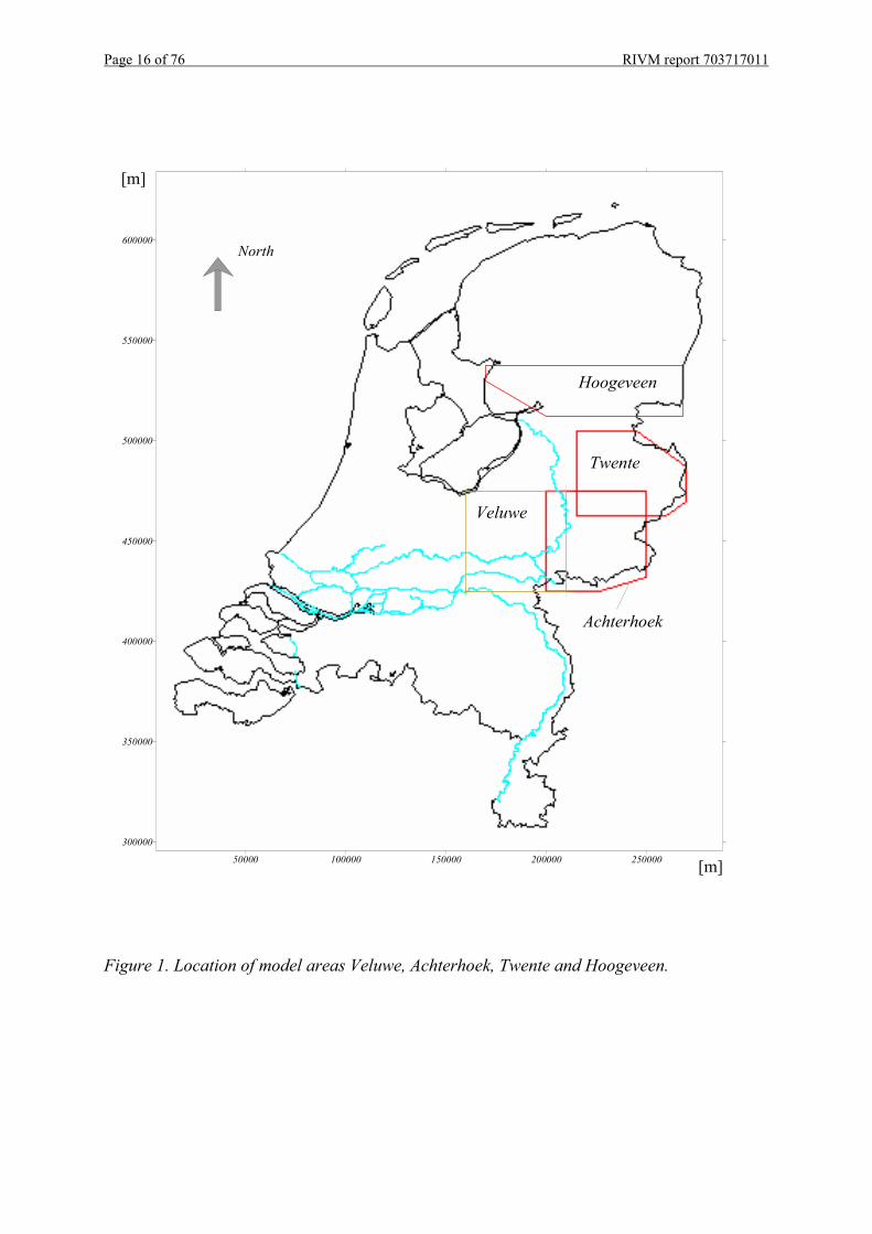
The study area is localised in the eastern and central part of the Netherlands (Figure 1). In thispart of the country the underground consists of sandy layers of Pleistocene origin. The totalthickness of the Pleistocene sand complex varies from 20 to 300 metres and more. In someparts semi-pervious clay layers occur that separate the Pleistocene formation into severalinteracting aquifers. Where the clay layers are absent the system reacts as a single phreaticaquifer. For the greater part the aquifer system is replenished by natural recharge, although insome areas seepage occurs. Mostly, the seepage is drained off by a system of ditches anddrainage tiles. In lower lying infiltration areas also a drainage system may be present. In thiscase part (or all) of the natural recharge may be drained off (see Chapter 5).
A characteristic feature of the study area is the presence of several ice-pushed ridges (Veluwe,Montferland, Nijverdal and Ootmarsum). These ridges were formed during the Saale ice age,during which the northeast and central part of the Netherlands was covered with ice.Typically, the ice pushed areas can be identified as good infiltration areas. Seepage is moreprevalent in the lower laying areas (IJssel-Valley).
The study area has been subdivided into several ‘subareas’, for each of which a separategroundwater model has been set up (Kovar et al., 1998). The subareas, named Achterhoek,Veluwe, Twente and Hoogeveen in the present report, coincide with the model areas ‘a2’,‘v2’, ‘t2’ and ‘h2’ respectively from Kovar’s study. The dimensions and coordinates of themodel areas are presented in Table 1. The areas Veluwe, Achterhoek and Twente partlyoverlap (Figure 1), while the Hoogeveen model is not connected to any of the other three. Inthe following sections, where the spatial distribution of various geohydrological parameters ispresented, the sub-areas are combined into one plot. Note that this results in two non-contiguous areas.
Table 1. Geometric Properties of the model areas.coordinates [km]Name of area Dimension [km2]
xmin xmax ymin ymax
Achterhoek 50 � 50 200 250 425 475Veluwe 50 � 50 160 210 425 475Twente 55 � 42.5 215 217 462.5 505Hoogeveen 98 � 25 170 268 512.5 537.5
Page 16 of 76 RIVM report 703717011
Figure 1. Location of model areas Veluwe, Achterhoek, Twente and Hoogeveen.
50000 100000 150000 200000 250000
300000
350000
400000
450000
500000
550000
600000
Twente
Achterhoek
Veluwe
Hoogeveen
[m]
[m]
North

RIVM report 703717011 Page 17 of 76
Figure 2 gives a three-dimensional view of the surface elevation with respect to Dutch datumlevel (NAP). The elevation varies between – 4 and 103 metres (NAP). Notice the presence ofseveral ice-pushed ridges, where the elevation is higher than the direct surroundings.
Figure 2. Three-dimensional view of the surface elevation.
(a) Veluwe(b) Montferland(c) Lochemerberg(d) Holterberg (Nijverdal)(e) Lonnekerberg (Oldenzaal)(f) Ootmarsum(g) Lemelerberg
(g)
(f)(e)
(d)
(c)
(b)(a)[m] [m]
[m]
North
Page 18 of 76 RIVM report 703717011
3.2 Surface waters
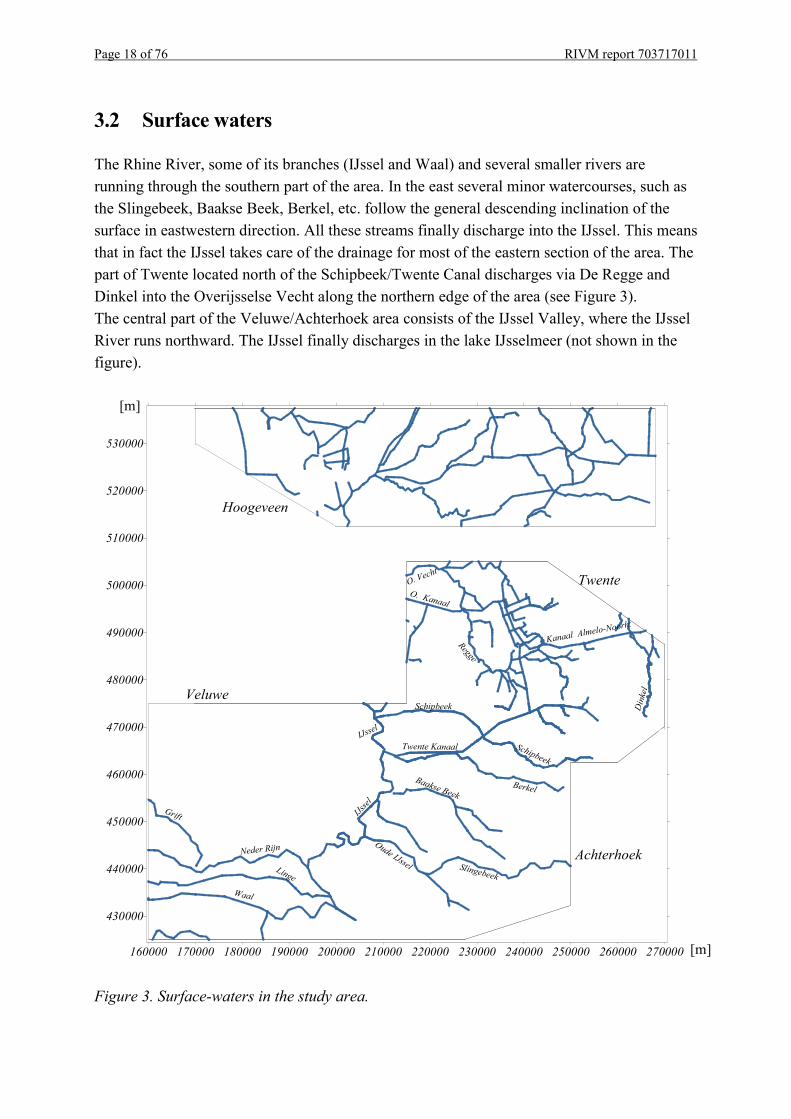
The Rhine River, some of its branches (IJssel and Waal) and several smaller rivers arerunning through the southern part of the area. In the east several minor watercourses, such asthe Slingebeek, Baakse Beek, Berkel, etc. follow the general descending inclination of thesurface in eastwestern direction. All these streams finally discharge into the IJssel. This meansthat in fact the IJssel takes care of the drainage for most of the eastern section of the area. Thepart of Twente located north of the Schipbeek/Twente Canal discharges via De Regge andDinkel into the Overijsselse Vecht along the northern edge of the area (see Figure 3).The central part of the Veluwe/Achterhoek area consists of the IJssel Valley, where the IJsselRiver runs northward. The IJssel finally discharges in the lake IJsselmeer (not shown in thefigure).
Figure 3. Surface-waters in the study area.
160000 170000 180000 190000 200000 210000 220000 230000 240000 250000 260000 270000
430000
440000
450000
460000
470000
480000
490000
500000
510000
520000
530000
IJssel
Slingebeek
Oude IJssel
Baakse BeekBerkel
Twente KanaalIJssel
Schipbeek Din
kel
Regge
O. Vecht
Schipbeek
O. Kanaal
Kanaal Almelo-Noorh.
Neder Rijn
Linge
Waal
Grift
[m]
[m]
Veluwe
Twente
Achterhoek
Hoogeveen

RIVM report 703717011 Page 19 of 76
3.3 Aquifer system
The thickness of the Pleistocene complex that comprises the aquifer system variesconsiderably. At the southeastern side the thickness is between 10 and 30 metres. In thenorthwestern direction the thickness increases to 300 metres and more. This is due to the rapiddecline of the low permeable Breda Formation, which is considered to be the base of thegeohydrological system. Figure 4 presents a contourmap of the base elevation. Detailedgeological descriptions of the area can be found in Grootjans (1984) and Vermeulen et al.(1996), as well as in the NAGROM/TNO report (Anonymous, 1993).
Figure 4. Contours of the base of the aquifer system.
170000 180000 190000 200000 210000 220000 230000 240000 250000 260000
430000
440000
450000
460000
470000
480000
490000
500000
510000
520000
530000
Depth in metres NAP (Dutch datum level)
[m]
[m]

Page 20 of 76 RIVM report 703717011
Figures 5 and 6 show the presence and thickness of the first (Eemian-clay) and secondaquitard (Drenthe/Tegelen-clay) as modelled in LGM.
Figure 5. Presence and thickness of the first aquitard (Eem-clay).
160000 170000 180000 190000 200000 210000 220000 230000 240000 250000 260000 270000
430000
440000
450000
460000
470000
480000
490000
500000
510000
520000
530000
01234567891011
Thickness first aquitard in metres
[m]
[m]

RIVM report 703717011 Page 21 of 76
Figure 6. Presence and thickness of second aquitard (Drenthe-clay).
160000 170000 180000 190000 200000 210000 220000 230000 240000 250000 260000 270000
430000
440000
450000
460000
470000
480000
490000
500000
510000
520000
530000
Thickness second aquitard in metres
036101520253035404550556065707580[m]
[m]
Page 22 of 76 RIVM report 703717011
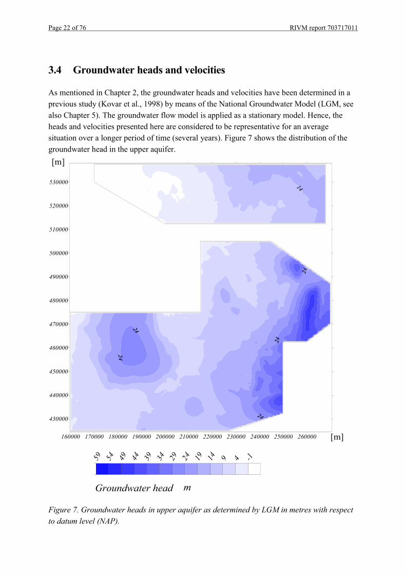
3.4 Groundwater heads and velocities
As mentioned in Chapter 2, the groundwater heads and velocities have been determined in aprevious study (Kovar et al., 1998) by means of the National Groundwater Model (LGM, seealso Chapter 5). The groundwater flow model is applied as a stationary model. Hence, theheads and velocities presented here are considered to be representative for an averagesituation over a longer period of time (several years). Figure 7 shows the distribution of thegroundwater head in the upper aquifer.
Figure 7. Groundwater heads in upper aquifer as determined by LGM in metres with respectto datum level (NAP).
-14914192429343944495459
Groundwater head
160000 170000 180000 190000 200000 210000 220000 230000 240000 250000 260000
430000
440000
450000
460000
470000
480000
490000
500000
510000
520000
530000
m
[m]
[m]
RIVM report 703717011 Page 23 of 76
This picture reflects the surface relief in a less pronounced manner. It shows a generaldecrease from the southeastern edge towards the IJssel valley in the central part. The higherheads under the ice-pushed Veluwe-hills in the southwest are clearly visible. Other ice-pushedridges (Montferland, Nijverdal, Ootmarsum and Oldenzaal) can also be observed andassociated with higher heads.
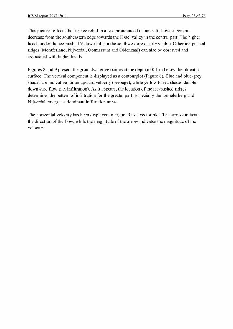
Figures 8 and 9 present the groundwater velocities at the depth of 0.1 m below the phreaticsurface. The vertical component is displayed as a contourplot (Figure 8). Blue and blue-greyshades are indicative for an upward velocity (seepage), while yellow to red shades denotedownward flow (i.e. infiltration). As it appears, the location of the ice-pushed ridgesdetermines the pattern of infiltration for the greater part. Especially the Lemelerberg andNijverdal emerge as dominant infiltration areas.
The horizontal velocity has been displayed in Figure 9 as a vector plot. The arrows indicatethe direction of the flow, while the magnitude of the arrow indicates the magnitude of thevelocity.

Page 24 of 76 RIVM report 703717011
Figure 8. Vertical groundwater velocity at 0.1 m below phreatic surface.
160000 170000 180000 190000 200000 210000 220000 230000 240000 250000 260000 270000
430000
440000
450000
460000
470000
480000
490000
500000
510000
520000
530000
-0.020
-0.016
-0.012
-0.008
-0.004
0.000
0.005
0.010
0.020
0.200
Infiltration (m/day)
[m]
[m]
Seepage (m/day)
RIVM report 703717011 Page 25 of 76
Figure 9. Direction and magnitude of horizontal groundwater velocities at 0.1 m below thephreatic surface.
160000 170000 180000 190000 200000 210000 220000 230000 240000 250000 260000 270000
430000
440000
450000
460000
470000
480000
490000
500000
510000
520000
530000
[m]
[m]
0.5 m/day
0.25 m/day

Page 26 of 76 RIVM report 703717011

RIVM report 703717011 Page 27 of 76
4 Groundwater abstraction
4.1 Rates of discharge
In the study area a large number of industrial wells and private groundwater abstractions arepresent as well as a number of pumping stations abstracting water for public drinking watersupply. The total groundwater abstraction for public water supply has increased substantiallyduring the period 1960-’80. Since then, the level of abstraction more or less remainedconstant, while after 1990 a slightly decreasing trend can be observed. Examples are shown inthe Figures 10 and 11. These graphs give the total amount of water (in million m3 year-1)abstracted for public water supply by the pumping stations in 2 of the 4 model areas.Industrial and private groundwater abstractions are not included in the graphs, but they aretaken into account in the model. In both areas (Achterhoek and Twente) the industrial andprivate abstractions are approximately 50% of the total abstracted volume.
Figure 10. Yearly abstracted volume of groundwater by pumping stations in model areaAchterhoek.
Groundwater Abstraction Achterhoek
0.0
10.0
20.0
30.0
40.0
50.0
1950
1953
1956
1959
1962
1965
1968
1971
1974
1977
1980
1983
1986
1989
1992
1995
1998
year
Volu
me
[M m
3 /y]

Page 28 of 76 RIVM report 703717011
Figure 11. Yearly abstracted volume of groundwater by pumping stations in model areaTwente.
4.2 Locations
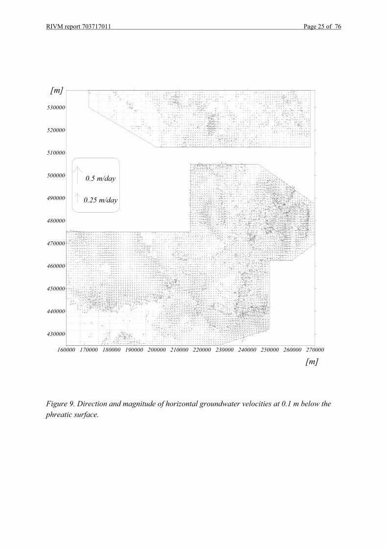
The locations of all groundwater abstractions are displayed in Figure 12. Private andindustrial abstraction wells (with a discharge larger than 50000 m3 year -1) are indicated as redcircles, while the public water supply pumping stations are shown as black circles. The sizesof these circles are proportional to the amount of abstraction. In the present report attention isfocused on 9 public water supply pumping stations, which were randomly selected throughoutthe central and eastern part of the Netherlands. In this part of the country the occurrence ofnitrate in groundwater is a topical subject. For the selected pumping stations also the capturezone is given in green (Figure 12).
Groundwater Abstraction Twente
0.0
10.0
20.0
30.0
40.0
50.0
1950
1953
1956
1959
1962
1965
1968
1971
1974
1977
1980
1983
1986
1989
1992
1995
1998
Year
Volu
me
[M m
3 /y]
RIVM report 703717011 Page 29 of 76
Figure 12. Location of the groundwater abstractions and the capture zones of selectedpumping stations.
160000 170000 180000 190000 200000 210000 220000 230000 240000 250000 260000 270000
430000
440000
450000
460000
470000
480000
490000
500000
510000
520000
530000
Klooster
De_Pol
Dinxperlo
Archemerberg
Nijverdal
Herikerberg
Wierden
Putten
Coevorden
[m]
[m]
Pumping Station
Private or IndustrialAbstraction
Capture zone

Page 30 of 76 RIVM report 703717011

RIVM report 703717011 Page 31 of 76
5 Data and models
5.1 Nitrate measurements
Parameter estimation or calibration is the process of fitting measured data with data generatedby the model that includes the unknown parameter(s). The set of nitrate measurements used inthis report may be divided into two categories. The first category consists of data frommonitoring wells (Monitor Well Data). These data originate from the National GroundwaterMonitoring Network, which has been installed during 1979-1984 (Snelting et al., 1990).Groundwater samples are collected at least annually at various filter depths (up to 30 metresbelow surface). The volume of the water samples is relatively small in comparison to thespatial resolution of the groundwater transport model. For, instance, a calculatedconcentration represents a volume 125 × 125 ×10 m3, while the measurements are based on avolume of several litres. Therefore, in practice, the measurements may be regarded as pointmeasurements. From detailed local studies it is known that nitrate levels fluctuate during theyear and vary considerably in space as well. The data used in this study are representative forfour moments in time, respectively the years 1982, 1990, 1995 and 2000. In order to obtainthe data in the right format, some pre-processing and averaging has been applied. For a certainmoment t the measurements are averaged over an interval starting at t - 500 days until t + 500days. In a few cases data from local monitoring networks have been added to the data set.
The second category of data (Breakthrough Data) consists of nitrate contents measured at thepumping stations. The main difference with the monitoring data is that breakthrough datarefer to a mixture of waters that have infiltrated at different locations and at different times.Therefore, this is a mixture of waters with different ages and origins. Nitrate measurements atthe pumping stations should preferably be taken from the water before the purificationprocess. For most pumping stations nitrate contents have been collected since 1992 in the so-called REWAB programme (in Dutch: REgistratie opgaven van WAterleidingBedrijven).These measurements refer to the untreated water as well as the water after purification. Alonger series of data is available from the LMD measuring programme (in Dutch: LandelijkMeetnet Drinkwaterkwaliteit), which refers to the nitrates of the water after the purification.In the purification process no specific nitrate decontamination is applied and in a number ofcases the measurements in the treated and untreated water hardly differ. However, this doesnot hold for all pumping stations.
5.2 Leachate model
At present STONE is being used as the standard tool in national scale nutrient leachingstudies. STONE (Beusen et al., 2000; Overbeek et al., 2001a) calculates the flux of several

Page 32 of 76 RIVM report 703717011
nutrients from the root zone into the groundwater system on a temporal basis of decades (10days). The spatial differentiation of the model results is obtained by applying the model for alarge number of unique combinations of soil type, land use and hydrological features. For thepresent study area nitrate leaching rates have been calculated by STONE within theframework of the fifth National Environmental Outlook. These are described in more detailby Overbeek et al. (2001b). The temporal resolution of 1 decade of days of the STONE data istoo detailed for the solute transport model. Therefore, the data have been transformed into 15-year averages for the interval from 1950-2000.
5.3 Groundwater model
As mentioned before, Kovar et al. (1998) calculated the groundwater heads and velocities inthe area with the groundwater flow model National Groundwater Model LGM (Pastoors,1992; Kovar et al., 1992). LGM is based on finite elements and describes the groundwaterflow in a multi-aquifer system separated by one or more aquitards. Within each aquifer thehead distribution is treated two-dimensionally in horizontal direction, while through theaquitards purely vertical flow is assumed. In terms of groundwater velocities the model isquasi-three-dimensional. The horizontal flow components are derived from Darcy’s low,while the vertical flow is obtained by an approximate procedure, known in the literature asStrack’s interpretation of Dupuit-Forchheimer (Strack, 1984). In short, the approximationmay be formulated as follows: within the aquifers vertical conductivity is assumed infinitelylarge, while in the aquitards the horizontal conductivity is assumed to be zero.
At the top of the upper aquifer, interaction occurs between the groundwater and the drainagesystem of ditches and drainage tiles. This zone is referred to as the top-system. In principlenatural recharge infiltrates at the phreatic surface. This vertical groundwater flux is denotedby qre. A portion of this recharge may leave the underground after a relatively short stay (e.g.several days) and discharge into the drainage system. The latter portion is referred to as thetop system discharge, denoted by qts. The top system discharge plays a role in thedetermination of the nitrate flux that reaches the groundwater.
The top system discharge is taken into account in the groundwater model via the followingexpression:
0ts
hqc
� �
� (1)
where the coefficient c is the so-called drainage resistance (days), 0h is the zero drainage
level (drainage base) and �(x,y) is the groundwater head as calculated by LGM. The amountof water infiltrating into the aquifer system, qas, is qre - qts or:

RIVM report 703717011 Page 33 of 76
0as re
hq qc
� �
� � (2)
Note that qre , h0 and c are all given input parameters, while both �(x,y) and also qas, need tobe calculated by the model. When � is greater than h0 , the aquifer system discharges waterinto the drainage system. Irrigation occurs when � is less than h0 , i.e. water infiltrates fromthe ditches and drains into the aquifer. Both h0 and c may vary in space, so qts also is afunction of the horizontal co-ordinates x and y. The parameters c, h0 and qre are all given asmodel input.
The drainage or irrigation that take place in the top-system is not only relevant for the massbalance of water, but also for the net amount of nitrate that finally enters the aquifer system.Together with the discharge qts an amount of nitrate is removed via the drainage system. Thisnitrate term must be taken into account. In case of infiltration/irrigation an additional amountof water enters the aquifer. The nitrate content of this term is unknown. In this study it isassumed to be zero.
Figure 13. Scheme of the Top-system.
In principle, LGM can be applied for non-stationary flow situations, but in the present andprevious studies steady conditions have been assumed. The recharge data represent rechargefrom the year 1988, which is considered to be a rather ‘wet’ year. Model parameters such asaquifer transmissivities and aquitard resistance have been calibrated on measured head data(Leijnse and Pastoors, 1996).

Page 34 of 76 RIVM report 703717011
5.4 Solute transport model
The next modelling step concerns the nitrate transport. The LGM-package includes the solutetransport module LGMCAD (Uffink, 1996, 1999). LGMCAD uses the particle trackingtechnique, which means that during the calculating process particles are introduced in theaquifer. The particles are characterised by several time dependent attributes, such as x, y and zco-ordinates and a (solute) mass m, here representing a certain amount of dissolved nitrate.The model calculates the displacement and mass changes for each particle separately. Theparticle displacement consists of a deterministic component that describes advective transportand a stochastic component that accounts for the dispersive transport. More information onthis modelling technique and its application in LGMCAD is found in Uffink (1990) andKinzelbach and Uffink (1991).
The main input data for the transport model are the (3D) groundwater velocity distribution forthe aquifer and the nitrate fluxes at the upper boundary. The groundwater velocity distributionis provided the groundwater flow module (LGMFLOW). Nitrate fluxes at the phreatic surfacehave been generated with the leaching model STONE. Observations show that in the verticaldirection steep nitrate concentration gradients occur. To retain such gradients in thesimulation, special attention is required to the simulation of vertical mixing processes.Numerical dispersion should be avoided by all means, since it would destroy all verticalresolution. The random walk particle technique is an effective procedure in this respect, sincenumerical dispersion is absent. Small vertical dispersivity values are used.
As stated earlier, nitrate transport in the aquifer can only be simulated when information isavailable on the amount of nitrate entering the aquifer from the unsaturated zone. Thisinformation forms the upper boundary condition in terms of solute fluxes. The leaching datagenerated by STONE need to be pre-processed before an adequate upper boundary conditioncan be set up. This is due to the rather complicated situation at the upper boundary (top-system) and the fact that STONE and LGM are based on different modelling concepts for thetop-system.
Schematically the situation is as follows. At the bottom of the unsaturated zone a hypotheticalsurface is considered, through which a downward groundwater flux qre(x, y) occurs. Since thegroundwater flow model is stationary, this term does not depend on time. When the nitrateconcentration is denoted by cN(x, y, t), the nitrate flux �re, through this surface is the productcN × qre. Note that contrary to the water flux, the nitrate flux does depend on time since theconcentrations depend on time. In the absence of the drainage system the product cN × qre
provides the upper boundary solute flux for the transport model. However, due to the drainagesystem, the actual water flux into the system, may be reduced to qas , as given by eq. (2), andthe solute flux becomes cN × qas. In fact, this product represents the coupling of the leaching

RIVM report 703717011 Page 35 of 76
and solute transport model, since cN is produced by STONE, while qas is determined byLGM. However, in the leaching model the situation is more complicated since it describes notonly the unsaturated zone, but also part of the saturated zone and thus part of the drainagesystem. Further, instead of the (stationary) hypothetical surface considered in the groundwaterwe have a fluctuating phreatic surface. Since the model concepts that are used are essentiallydifferent, it is not directly clear what depth must be chosen to couple the two models. In thepresent study we use the STONE data at the so-called GHG-level (mean highest groundwaterhead). This level is a standard depth for the STONE output. Overestimated nitrate flux may beexpected when these data are used, since nitrate concentrations demonstrate a rapid decreasewith depth between GHG-level and GLG-level (mean lowest groundwater head). Evendirectly below GLG-level a rapid decrease of nitrates occurs. Overbeek et al. (2001b) havereported a nitrate reduction with 20-25% in the first 0,5 meter below GLG. Theoverestimation in the nitrate flux may be compensated when a reduction factor or zero-orderdenitrification concept is included in the denitrification module. This is described in moredetail in Chapter 6.

Page 36 of 76 RIVM report 703717011
RIVM report 703717011 Page 37 of 76
6 Denitrification
6.1 General
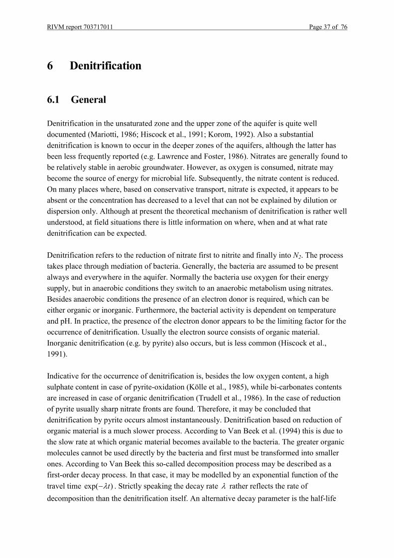
Denitrification in the unsaturated zone and the upper zone of the aquifer is quite welldocumented (Mariotti, 1986; Hiscock et al., 1991; Korom, 1992). Also a substantialdenitrification is known to occur in the deeper zones of the aquifers, although the latter hasbeen less frequently reported (e.g. Lawrence and Foster, 1986). Nitrates are generally found tobe relatively stable in aerobic groundwater. However, as oxygen is consumed, nitrate maybecome the source of energy for microbial life. Subsequently, the nitrate content is reduced.On many places where, based on conservative transport, nitrate is expected, it appears to beabsent or the concentration has decreased to a level that can not be explained by dilution ordispersion only. Although at present the theoretical mechanism of denitrification is rather wellunderstood, at field situations there is little information on where, when and at what ratedenitrification can be expected.
Denitrification refers to the reduction of nitrate first to nitrite and finally into N2. The processtakes place through mediation of bacteria. Generally, the bacteria are assumed to be presentalways and everywhere in the aquifer. Normally the bacteria use oxygen for their energysupply, but in anaerobic conditions they switch to an anaerobic metabolism using nitrates.Besides anaerobic conditions the presence of an electron donor is required, which can beeither organic or inorganic. Furthermore, the bacterial activity is dependent on temperatureand pH. In practice, the presence of the electron donor appears to be the limiting factor for theoccurrence of denitrification. Usually the electron source consists of organic material.Inorganic denitrification (e.g. by pyrite) also occurs, but is less common (Hiscock et al.,1991).
Indicative for the occurrence of denitrification is, besides the low oxygen content, a highsulphate content in case of pyrite-oxidation (Kölle et al., 1985), while bi-carbonates contentsare increased in case of organic denitrification (Trudell et al., 1986). In the case of reductionof pyrite usually sharp nitrate fronts are found. Therefore, it may be concluded thatdenitrification by pyrite occurs almost instantaneously. Denitrification based on reduction oforganic material is a much slower process. According to Van Beek et al. (1994) this is due tothe slow rate at which organic material becomes available to the bacteria. The greater organicmolecules cannot be used directly by the bacteria and first must be transformed into smallerones. According to Van Beek this so-called decomposition process may be described as afirst-order decay process. In that case, it may be modelled by an exponential function of thetravel time exp( )t�� . Strictly speaking the decay rate � rather reflects the rate ofdecomposition than the denitrification itself. An alternative decay parameter is the half-life

Page 38 of 76 RIVM report 703717011
time, ½T , which expresses the time needed to reduce the initial concentration by a factor ½.Half-life time and decay rate are related by
½ln 2 0.7T� �
� � (3)
Especially in artificial denitrification projects the biodegradation process has been studiedintensively. Artificial denitrification is a technique where on purpose nitrates are added to thegroundwater in order to stimulate the bacteria in their degradation process. In those cases thefinal objective is to reduce the amount of organic contaminants. Often, in these studies thekinetics are described by the so-called Monod equation, which is of the following form:
dc cadt K c
� �
�
(4)
where K and a are constants. Mathematically, this non-linear equation is difficult to model,but for low concentrations ( c K� ) it may be approximated by a first-order (exponential)equation (Bekins et al., 1998):
dc a cdt K
� � (5)
For higher concentrations, however, the first order approximation leads to an overestimatednitrate reduction.
6.2 Implementation
A first order decay process is easy to implement in a solute transport code that applies particletracking. Uffink and Römkens (2001) have obtained experience with the exponentialdenitrification model. It appeared that results obtained with a single decay parameter (nozones) were not satisfactory. Therefore a spatial (zonal) distribution of the parameter wasproposed. At first a constant ‘background’ value is assigned everywhere in the aquifer system.This value is changed in a zone of 5 metre directly above and beneath the major clay-layers(aquitards) and in the direct vicinity of local streams and rivers. The reasoning behind thisapproach is that in these zones more organic material is present and therefore a higherdenitrification capacity may be expected. For instance Meinardi (1999) has observed in astudy area in the Achterhoek (Hupsel) that denitrification occurs when the deep groundwateris in contact with the clay inclusions at the base of the aquifer. The decay-parameters foundby Uffink and Römkens, expressed as half-life times, are ranging from 200 to 2000 days.
In the present transport model, besides a first order decay, an additional type of denitrificationhas been implemented. Directly after the groundwater (and nitrate) has entered the aquifer an
RIVM report 703717011 Page 39 of 76
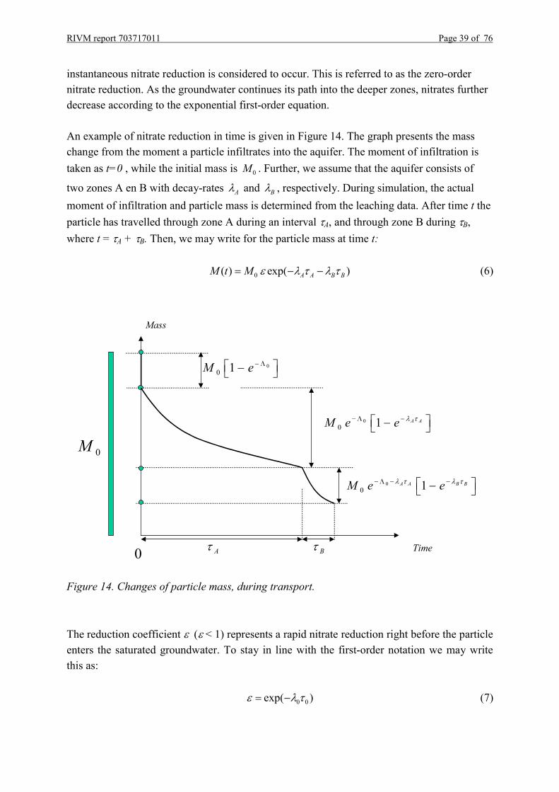
instantaneous nitrate reduction is considered to occur. This is referred to as the zero-ordernitrate reduction. As the groundwater continues its path into the deeper zones, nitrates furtherdecrease according to the exponential first-order equation.
An example of nitrate reduction in time is given in Figure 14. The graph presents the masschange from the moment a particle infiltrates into the aquifer. The moment of infiltration istaken as t=0 , while the initial mass is 0M . Further, we assume that the aquifer consists of
two zones A en B with decay-rates A� and B� , respectively. During simulation, the actualmoment of infiltration and particle mass is determined from the leaching data. After time t theparticle has travelled through zone A during an interval �A, and through zone B during �B,where t = �A + �B. Then, we may write for the particle mass at time t:
0( ) exp( )A A B BM t M � � � � �� � � (6)
Figure 14. Changes of particle mass, during transport.
The reduction coefficient � (� < 1) represents a rapid nitrate reduction right before the particleenters the saturated groundwater. To stay in line with the first-order notation we may writethis as:
0 0exp( )� � �� � (7)
00 1M e ��� ��� �
Time
0M
00 1A A B BM e e� � � ��� � �� ��� �
00 1 A AM e e � �� � �� ��� �
Mass
A� B�0

Page 40 of 76 RIVM report 703717011
where �0 is a (high) denitrification rate that is supposed to occur in a very short time �0. Theconcept of a zero order denitrification implies that the product 00�� remains constant when
��� 00 ,0 �� . So, with 00���0Λ this leads to:
0 0( ) exp( )A A B BM t M Λ � � � �� � � � (8)
The concept of exponential decay has also been applied by Wendland (1992) to describedenitrification in similar aquifer types in Germany. However, the decay parameter � shouldnot be associated too closely with the actual denitrification processes. According to Van Beeket al. (1984) it also reflects the decomposition process of the organic material. This alsomeans that its value may not be derived directly from soil-parameters. So far, values can bestbe guessed or, when data from measurements are available, determined by calibrationtechniques, as is done in the present report. Obermann (1982) has applied a reduction factor,similar to the zero order term proposed here. For the lower Rhine region in Germany factorsare reported of 0.16, 0.63 and 0.70 (Haag and Kaupenjohann, 2001).
For the spatial distribution of the exponential decay rates a zonal approach is applied, whichmeans that in the model area two zones are defined. One zone covers a default or backgroundzone, where the decay rate is considered to be low. Then, in the aquifer system a second zoneis identified, where the decay rate is expected to be higher, e.g. because it may be expectedthat in this zone more organic material is present. For the present study the high decay rate isapplied in a layer of 5-metre thickness above and underneath the claylayer (first aquitard) andin all gridcells adjacent to rivers and minor courses of surface water. The same distributionscheme has been used in Uffink and Römkens (2001) as well as in Uffink and Mülschlegel(2002). The location of the surface water and rivers has been displayed in section 3.2, whilethe occurrence of the claylayers has been presented in section 3.3.
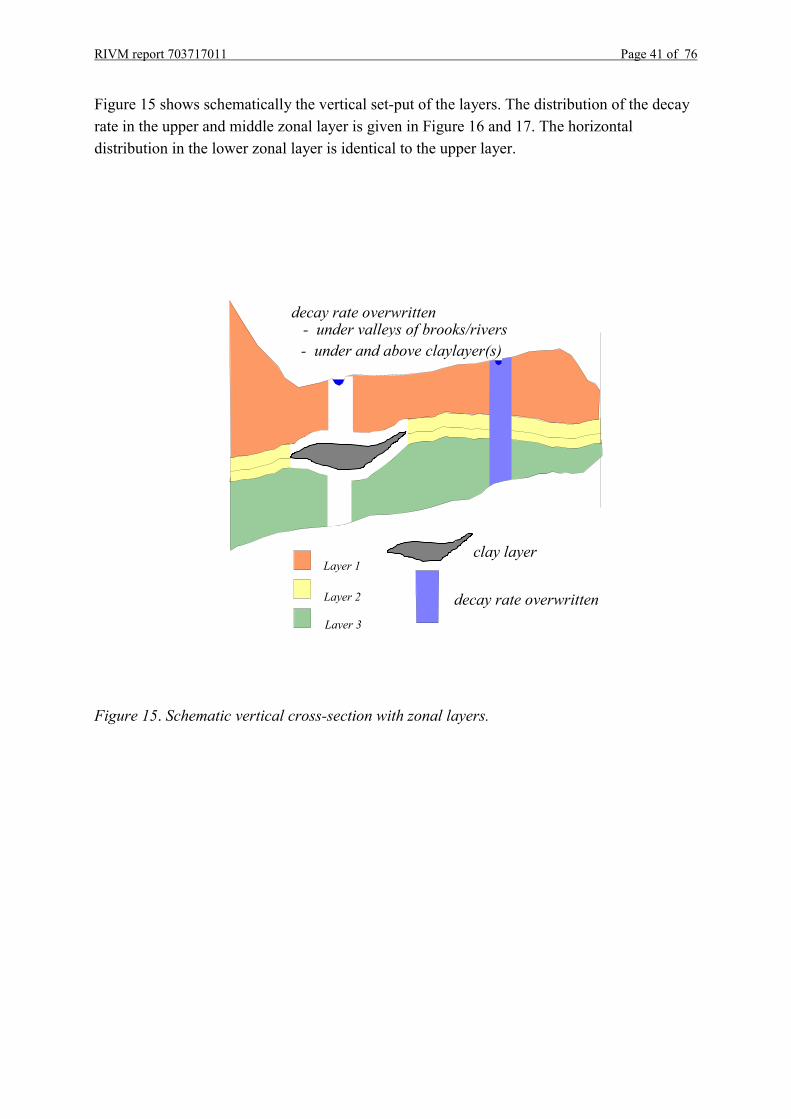
Finally, a spatial pattern emerges that in vertical direction is composed of three layers. Withineach layer a regular grid with 500 x 500 m cells is defined. In each gridcell the decay rate iseither equal to A� or B� . The allocation of the decay rate depends on whether a claylayer ispresent or not, or whether the cell is underneath a river or stream. The elevation and thicknessof the middle zonal layer is directly related to the Drenthe-clay-layer. In case clay is present,the layer is defined between 5 metres above the top of the clay until 5 metres underneath thebottom. At those location where the clay is absent the actual elevation of the layer is notrelevant since here no distinction between the layers exists. The upper zonal layer extendsvertically from the surface to the top of the middle layer, while the lower zonal layer runsfrom the bottom of the middle layer to the base of the aquifer system.
RIVM report 703717011 Page 41 of 76
Figure 15 shows schematically the vertical set-put of the layers. The distribution of the decayrate in the upper and middle zonal layer is given in Figure 16 and 17. The horizontaldistribution in the lower zonal layer is identical to the upper layer.
Figure 15. Schematic vertical cross-section with zonal layers.
Layer 1
Layer 2
Layer 3
decay rate overwritten
decay rate overwritten- under valleys of brooks/rivers- under and above claylayer(s)
clay layer

Page 42 of 76 RIVM report 703717011
Figure 16. Zonation for calibration of decay rate in layer 1 and 3.
160000 170000 180000 190000 200000 210000 220000 230000 240000 250000 260000 270000
430000
440000
450000
460000
470000
480000
490000
500000
510000
520000
530000
layer 1 and 3
[m]
[m]

RIVM report 703717011 Page 43 of 76
Figure 17. Zonation for calibration of decay rate in layer 2.
160000 170000 180000 190000 200000 210000 220000 230000 240000 250000 260000 270000
430000
440000
450000
460000
470000
480000
490000
500000
510000
520000
530000
[m]
[m]

Page 44 of 76 RIVM report 703717011
RIVM report 703717011 Page 45 of 76
7 Calibration
7.1 Parameters
The parameters to be estimated during the calibration procedure are the denitrificationconstants �0 , λA and λB , as given in equation (6). In the simulation programme, however,these parameters are given in an alternative notation [see eq. (3) and (5)]:
- ε : zero order reduction term [-]- ½
AT first order decay-rate, zone A [T]:- ½
BT first order decay-rate, zone B [T]
In this pilot study nine pumping stations have been selected (sect 4.2, Figure 12). For eachselected pumping station a separate calibration exercise is performed using nitratemeasurements from the monitoring wells located in a 20� 20 km2 area around the pumping-station and the breakthrough data from the pumping well itself. Hence, for each pumpingstation a separate set of the parameters given above is obtained. These parameter values arerepresentative only for the area around the pumping station. Note that the monitoring wells donot exclusively lie inside the capture zone and, consequently, the representative area is notrestricted to the capture zone.
7.2 Log transform of concentrations
During a calibration procedure the unknown model parameters are varied, while for each setof values the match between measured data and model outcomes is examined. The parametersthat yield the ‘best’ match between model results and measurements are considered as the bestestimates. Calibration has been applied successfully to estimate the aquifer transmissivitiesand hydraulic resistances of aquitards for the groundwater flow model (LGM) for theNetherlands (Leijnse and Pastoors, 1996). Leijnse and Pastoors used observed groundwaterheads for their calibration. For the present problem observed groundwater heads are useless,since the unknown denitrification parameters do not affect groundwater heads. For the presentcalibration exercise the most adequate data consist of measurements of groundwater nitrateconcentrations. The user still is still free to choose in what way measured and observed dataare expressed, e.g. linear or logarithmic.
The magnitude of the measured nitrated values varies within a wide range. Therefore, acalibration based on the ratios between predicted and measured concentration (or differencesof the logarithms of the concentrations) makes more sense than using the concentration

Page 46 of 76 RIVM report 703717011
differences directly. The effect of the log-transform is best illustrated by the simple example.Consider two monitoring wells A and B. In well A measured and calculated concentrationsare, respectively 102 and 103, while in well B measured and calculated concentrations are 2and 3. When the difference between measurements and model values to determine thegoodness of the match, it appears that the match is equally well for both wells. However,when we want to expressed that at well A the calculated value is less than 1% off, while atwell B the model outcome is 50% larger than the measured value, we need to considerlogarithms of measured and calculated values. In general, if one is interested in relative errorsrather than absolute errors it is more natural to consider the logarithm of the model outcomesand measurements. In this study we consider the log-transformed concentrations, since we aredealing with a wide range of concentration values and a relative error seems more relevantthan an absolute error:
lnm mi iY c� (9)
lnc ci iY c� (10)
Superscript m (measured) and c are used for observations and calculated values, respectively.The index i denotes an individual measurement, while ci
c represents the calculatedconcentration at the place and time of the ith measurement. The difference between measuredvalue and model outcome at location i is known as the residual. During the calibrationprocedure an objective function E is optimised, which is defined as the sum of the weighted(squared) residuals:
� �2
1,
Nm c
i i ii
E Y Y�
�
� �� (11)
where γi denotes a weight factor and N is the total number of observations. Weights may beused to express the importance of an observation with respect to the rest of the measurements.Weights may be used in various ways to control and manipulate the calibration process. Forinstance if one wants to exclude a particular observation from it calibration process, eithertemporarily or permanently, this can be achieved by a weight factor of zero. The objectivefunction E may be optimised by techniques such as Gauss-Marquardt-Levenberg method. Forfurther details see e.g. Cooley (1983) or Hill (1992).
7.3 Software
Calibration is performed with the programme PEST (Parameter Estimation). PEST is a modelindependent parameter optimisation programme developed by Doherty of WatermarkComputing (Doherty and Johnston, 2003). It is widely used in several fields including the

RIVM report 703717011 Page 47 of 76
field of groundwater flow. It uses a non-linear optimisation technique, based on the Gauss-Marquardt-Levenberg method. Various versions of PEST exist, both commercial and free (butlimited) versions. In this study a freeware version has been used that runs on a DOS platform.(Anonymous, 1994). The groundwater nitrate transport simulations, however, are running onUNIX machines. Several tools and scripts have been written to handle command switchesbetween the PC and UNIX machines. The advantage of the use of PEST is that the simulationprogramme itself does not have to be modified to perform the calibration. A disadvantage isthat the programme PEST is used as a ‘black box’. For instance, intermediate results of thecalibration process, such as the sensitivity matrix, are not given as output and remaininaccessible. In the present study e.g., the sensitivities would have provided usefulinformation to obtain a stable calibration procedure (see 7.4).
7.4 Procedure
Preliminary runs showed that calibration based on breakthrough data alone did not lead to aunique set of decay-parameters. When only the breakthrough data are used a so-called ill-posed problem arises. The system becomes better defined, when –in addition to thebreakthrough data– measurements from the monitoring wells are included. Problems due tothe ‘ill-posed-ness’ may be circumvented by using a step-wise calibration procedure. At eachstep only a single parameter is free to be varied, while the other are kept constant. Onlyobservations are used with a high sensitivity to the free parameter. For this approachinformation on the sensitivity matrix would be helpful. As mentioned above, PEST does notprovide this information. As an alternative, observations have been selected based on a moreintuitive argument. This has led to the following step-wise procedure.
– Step 1. First, a calibration run is performed without the breakthrough data using onlymonitor well measurements from the shallow filters. Switching off the breakthrough datacan be realised easily by setting the weights equal to zero. The purpose of the first run isto calibrate the zero-order decay term. The nitrate levels measured at shallow depth arethe most affected by the zero-order parameter, since the residence times are still relativelyshort and the first-order decay has not been active very long. In this step, only the zero-order and one of the first-order (the fast one) are allowed to vary. The slow exponentialdecay is set at a constant value ( ½
AT is 5000 days).– Step 2. Accordingly, the zero-order reduction parameter is frozen at the level found in
step 1. Both shallow and deep monitoring data are included, while we calibrate only thetwo exponential decay parameters. The results of this run are given in the appendix.
– Step 3. All observations are included. In the final step all parameters are allowed to vary,but the ratio between ½
AT and ½BT is kept constant at the value found in step 2.

Page 48 of 76 RIVM report 703717011

RIVM report 703717011 Page 49 of 76
8 Results
8.1 Calibration results
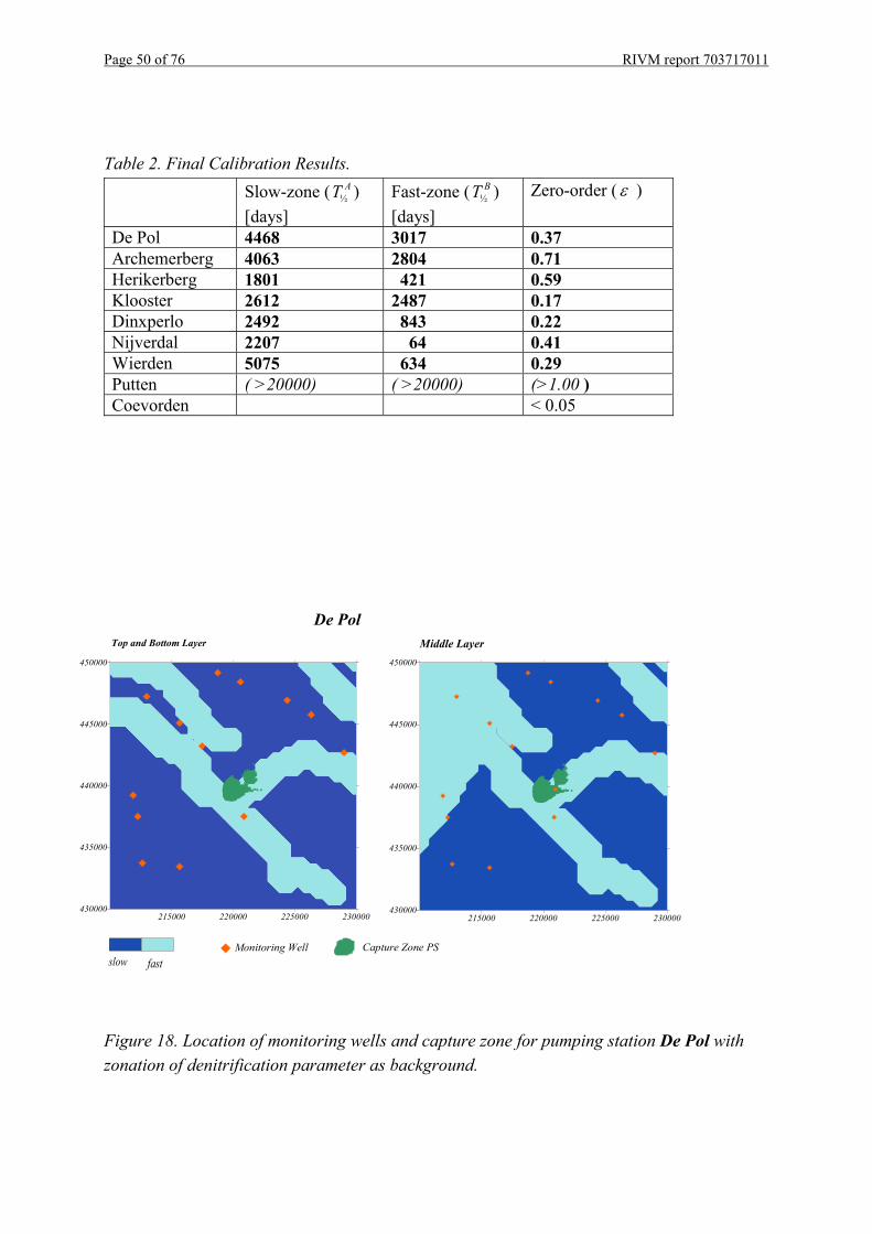
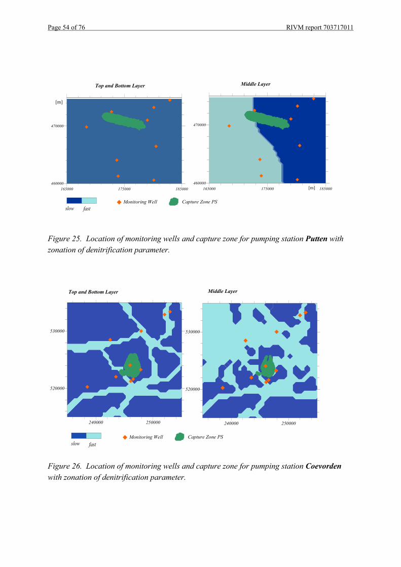
The transport model LGMCAD combined with PEST has been applied for a 20�20 km2 areaaround each selected pumping station. The Figures 18 to 26 give the location of themonitoring wells and capture zone of the pumping station projected on a map of the zonaldistribution of the decay parameter. The figures at the left-hand side give the zonaldistribution of the layers 1 and 3 (upper and bottom layer), while at the right-hand side figuresshow the zonation in layer 2 (middle layer). Note that the middle layer encloses the clay-layer(aquitard). The zonal distribution in this layer only differs from the one in the top layer at theplaces where the clay layer indeed exists. For each pumping station a set of parameter valueshas been obtained. The final results are given in Table 2. For the pumping station Putten thefinal denitrification values could not be obtained. In principle it may be concluded that atPutten no denitrification occurs. The model residuals for the pumping well data remainpositive, even for extremely high values of the half-life time (very slow denitrification) and azero-order reduction factor equal to 1.0. In terms of nitrates a positive residual says that modelresult shows less nitrate than is observed in the real system. In fact, when the zero-orderreduction factor is not bounded by an upper limit of 1.0, a value of 1.4 is obtained. This maybe an indication that nitrate fluxes are underestimated, while it also demonstrates that theinstantaneous (zero-order) reduction does not occur here. At pumping station Klooster thevalues for the two zones appear to be essentially the same. For an explanation refer to Figure21. In this figure it is seen that most of the shallow monitoring filters and the entire capturezone of the pumping wells are located in one and the same zone (zone A). Only a fewmonitoring wells are located in zone B, but very near to the border between the two zones.Note that the exact borders are drawn somewhat arbitrarily. Therefore, for this particular partof zone B a really faster decay parameter is not likely. It may be concluded that this area infact belongs to zone A. At the pumping station Coevorden the breakthrough data for nitrateare extremely low. Almost all nitrate appears to be removed by denitrification (see also sect.8.4). The calibration procedure results in a zero order reduction rate of 5%. However, it isdoubtful whether this is a realistic, physical value. A final set of half-life times could not beobtained here.
Page 50 of 76 RIVM report 703717011
Table 2. Final Calibration Results.Slow-zone ( ½
AT )[days]
Fast-zone ( ½BT )
[days]Zero-order (� )
De Pol 4468 3017 0.37Archemerberg 4063 2804 0.71Herikerberg 1801 421 0.59Klooster 2612 2487 0.17Dinxperlo 2492 843 0.22Nijverdal 2207 64 0.41Wierden 5075 634 0.29Putten ( >20000) ( >20000) (>1.00 )Coevorden < 0.05
Figure 18. Location of monitoring wells and capture zone for pumping station De Pol withzonation of denitrification parameter as background.
215000 220000 225000 230000430000
435000
440000
445000
450000
slow fast
Middle Layer
215000 220000 225000 230000430000
435000
440000
445000
450000
Monitoring Well
Top and Bottom Layer
Capture Zone PS
De Pol
RIVM report 703717011 Page 51 of 76
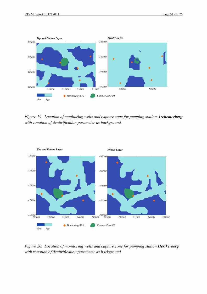
Figure 19. Location of monitoring wells and capture zone for pumping station Archemerbergwith zonation of denitrification parameter as background.
Figure 20. Location of monitoring wells and capture zone for pumping station Herikerbergwith zonation of denitrification parameter as background.
slow fast
Middle Layer
Monitoring Well Capture Zone PS
225000 230000 235000 240000 245000465000
470000
475000
480000
485000
225000 230000 235000 240000 245000465000
470000
475000
480000
485000
Top and Bottom Layer
slow fast
Middle Layer
Monitoring Well Capture Zone PS
220000 225000 230000 235000490000
495000
500000
505000
220000 230000490000
495000
500000
505000Top and Bottom Layer
Page 52 of 76 RIVM report 703717011
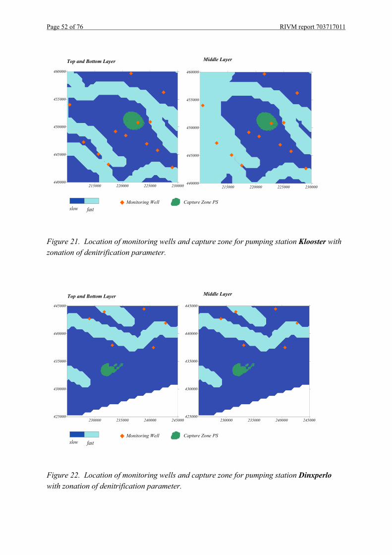
Figure 21. Location of monitoring wells and capture zone for pumping station Klooster withzonation of denitrification parameter.
Figure 22. Location of monitoring wells and capture zone for pumping station Dinxperlowith zonation of denitrification parameter.
slow fast
Middle Layer
Monitoring Well Capture Zone PS
215000 220000 225000 230000440000
445000
450000
455000
460000
215000 220000 225000 230000440000
445000
450000
455000
460000
Top and Bottom Layer
slow fast
Middle Layer
Monitoring Well Capture Zone PS
230000 235000 240000 245000425000
430000
435000
440000
445000
230000 235000 240000 245000425000
430000
435000
440000
445000
Top and Bottom Layer
RIVM report 703717011 Page 53 of 76
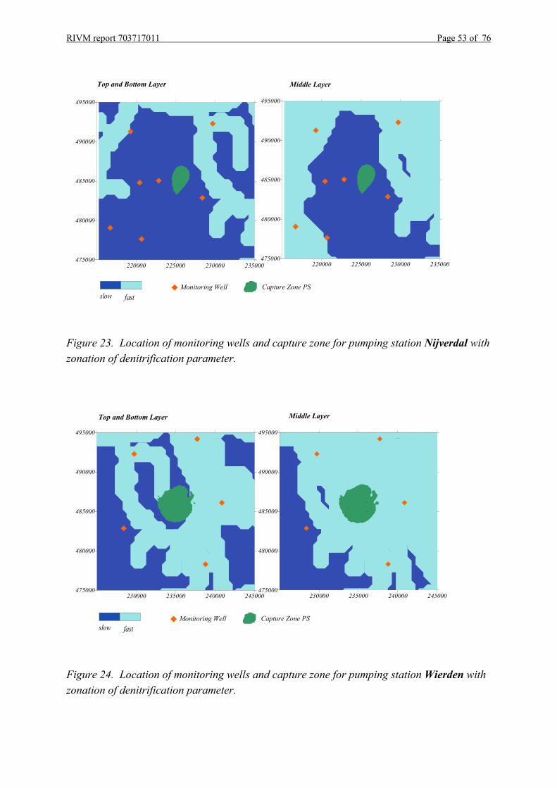
Figure 23. Location of monitoring wells and capture zone for pumping station Nijverdal withzonation of denitrification parameter.
Figure 24. Location of monitoring wells and capture zone for pumping station Wierden withzonation of denitrification parameter.
slow fast
Middle Layer
Monitoring Well Capture Zone PS
220000 225000 230000 235000475000
480000
485000
490000
495000
220000 225000 230000 235000475000
480000
485000
490000
495000
Top and Bottom Layer
slow fast
Middle Layer
Monitoring Well Capture Zone PS
230000 235000 240000 245000475000
480000
485000
490000
495000
230000 235000 240000 245000475000
480000
485000
490000
495000
Top and Bottom Layer
Page 54 of 76 RIVM report 703717011
Figure 25. Location of monitoring wells and capture zone for pumping station Putten withzonation of denitrification parameter.
Figure 26. Location of monitoring wells and capture zone for pumping station Coevordenwith zonation of denitrification parameter.
slow fast
Middle Layer
Monitoring Well Capture Zone PS
165000 175000 185000460000
470000
[m]
165000 175000 185000460000
470000
[m]
Top and Bottom Layer
slow fast
Middle Layer
Monitoring Well Capture Zone PS
240000 250000
520000
530000
240000 250000
520000
530000
Top and Bottom Layer
RIVM report 703717011 Page 55 of 76
8.2 Uncertainty
An indication for the parameter uncertainty can be obtained from the confidence limits. The95% confidence limits, as calculated by PEST, are given in Table 3. Note that these limits arebased on the assumption that the probability distribution of the parameters is normal and themodel is linear. Clearly, this assumption is not satisfied and consequently, at several cases thelimits have physically impossible values (negative half-life times and negative reductionfactors). Nevertheless, as a rough indication for the measure of uncertainty one may take theratio between the bandwidth (difference between upper and lower limit) and the parametervalue. For most cases shown in Table 3 the bandwidth is approximately two times theparameter itself.
At pumping station Dinxperlo the uncertainty appears to be much higher than average for thehalf-life time in zone B ( ½
BT ), while at the same time the uncertainty for ½AT is considerably
lower. An explanation may be obtained by examining Figure 22. It appears that most of themonitoring wells and the entire capture zone are located in zone A. Therefore, the value of ½
BTis not likely to affect the model results. This lack of sensitivity translates to a wide bandwidthfor this parameter. A similar argument holds for the situation around pumping station De Pol.
In general the uncertainty in the parameters is quite large. In this respect it must be mentionedthat the parameter uncertainty not only reflects the reliability of the observations. It also leadsback to the incompleteness of the model concept and to the uncertainty of other modelparameters and input data. For instance, the groundwater model has been treated as a steadystate system. However, over the simulation period (from 1950 to 2000) the actualhydrological situation around the pumping stations has not been constant. This is best seenfrom the development of the abstraction rates of the pumping stations in the Figure 10 and 11.Further, nitrate fluxes that enter the aquifer represent long time averages. Therefore, seasonalvariations, –still present in the shallow monitoring data– are absent in the model results.Another source of uncertainty is related to the transmissivities and hydraulic resistances usedin the flow model. These parameters have been calibrated with head measurements. It hasbeen mentioned earlier that groundwater heads do not depend on the denitrificationparameters. Conversely, the nitrate concentrations do depend on the transmissivities andhydraulic resistances. An integrated calibration procedure to obtain hydraulic parameters anddenitrification constants simultaneously should be preferred, but this is still quite an ambitiousexercise. A similar argument hold for the nitrate leaching data as provided by the modelSTONE. Finally, a source of uncertainty exists that is inherent to the technique used for thesolute transport simulation. The simulation is done by the random walk method, whichintroduces particles that are tracked through the system. The particle motion equations consistof a deterministic and a stochastic component. Due to this stochastic component, always some‘noise’ exists in the model outcomes. Using a large number of particles can reduce the level of

Page 56 of 76 RIVM report 703717011
noise, but this increases computational time. Therefore, in general a certain amount of ‘noise’is always accepted.
Table 3. The 95 % Confidence LimitsDe Pol Slow-zone ( ½
AT ) Fast-zone ( ½BT ) Zero-order (� )
lower limit 2310 days 1560 days 0.08value 4468 days 3017 days 0.37upper limit 6626 days 4474 days 0.66
Archemerberg Slow-zone ( ½AT ) Fast-zone ( ½
BT ) Zero-order (� )lower limit 2713 days 1872 days 0.15value 4063 days 2804 days 0.77upper limit 5413 days 3735 days 1.4
Herikerberg Slow-zone ( ½AT ) Fast-zone ( ½
BT ) Zero-order (� )lower limit 646 days 199 days 0.40value 1802 days 421 days 0.59upper limit 2952 days 642 days 0.79
Klooster Slow-zone ( ½AT ) Fast-zone ( ½
BT ) Zero-order ( 0� )lower limit 1769 days 1687 days -0.37value 2612 days 2487 days 0.17upper limit 3454 days 3287 days 0.72
Dinxperlo Slow-zone ( ½AT ) Fast-zone ( ½
BT ) Zero-order ( 0� )lower limit 2028 days -2623 days -value 2492 days 843 days 0.22upper limit 2956 days 4309 days -
Nijverdal Slow-zone ( ½AT ) Fast-zone ( ½
BT ) Zero-order ( 0� )lower limit -2377 days -69 days -0.07value 2207 days 64 days 0.41upper limit 6791 days 197 days 0.89
Wierden Slow-zone ( ½AT ) Fast-zone ( ½
BT ) Zero-order ( 0� )lower limit 494 days 62 days -0.18value 5075 days 634 days 0.29upper limit 9655 days 1206 days 0.75

RIVM report 703717011 Page 57 of 76
Putten Slow-zone ( ½AT ) Fast-zone ( ½
BT ) Zero-order ( 0� )lower limit - days - days -value - days - days -upper limit - days - days -
Coevorden Slow-zone ( ½AT ) Fast-zone ( ½
BT ) Zero-order ( 0� )lower limit - days days -0.18value - days - days 0.05upper limit - days days 0.75
8.3 Spatial distribution
With respect to the spatial variation the logarithm of the half-life time ½T is considered ratherthan the parameter itself. The logarithm of the parameter is a more natural quantity toexamine, since ½T should be a non-negative quantity. For the so-called slow-zone (zone A) anaverage half-life time ( ½
AT ) of 2745 days is found with a 65% interval ranging from1680 to 4450 days. This is slightly higher than the range from 3 to 5 years as reported byUffink and Römkens (2001). The difference may be due to the fact that Uffink and Römkensdid not include a separate zero-order denitrification concept.
The decay zone B (fast decay-zone) yields a mean value for ½BT of 745 days and a 65%
interval ranging from 225 to 2470 days. When pumping stations De Pol and Klooster areexcluded – at these locations the fast zone is not essentially different from the slow-zone - oneobtains a mean value of 495 days and a range between 165 and 1485 days. Uffink andRömkens reported for this zone a value ranging from 1 to 2 years.
The ‘instantaneous’ denitrification, which is supposed to occur in the region near the phreaticsurface, is a complicated factor. Besides a real physical process the factor represent also acompensation for a potential overestimation of the nitrate-input rates at the phreatic surface.Overbeek et al. (2001b) already pointed out that for dry sandy areas the leaching modelSTONE gives a 30% higher nitrate flux than similar models. One must be aware that allpotential errors in the nitrate fluxes eventually end up in the zero order reduction term.Therefore, a direct physical interpretation of the reduction factor must be avoided. Theaverage value for � amounts to 0.47 with a 65% range between 0.14 and 0.80. With respectto the average figure of 0.47 it is remarkable that Uffink and Mülschlegel (2002) mention areduction factor of 0.4 to be applied when nitrate fluxes generated by STONE are comparedto fluxes obtained by Van Drecht (1993) and Boumans and Van Drecht (1998).

Page 58 of 76 RIVM report 703717011
8.4 Match of observed and calculated breakthrough curves
For a few pumping stations the final simulated breakthrough curves are given together withthe measured data (Figures 27 to 31). Several comments can be made on these graphs.
– Herikerberg.The graph in Figure 27 gives both the raw water data (untreated water) and purified waterdata. Since the year 1992 data from both measuring programmes are available. ForHerikerberg, the nitrate contents of the treated and untreated water are clearlysubstantially different. Apparently during the purification process nitrates are removed.For the calibration process the LMD data have been discarded and only the data onuntreated water have been used
– Dinxperlo.The breakthrough curve for Dinxperlo is given in Figure 28. With respect to the measureddata there seems to be no systematic difference between the data for raw water andpurified water. Therefore, there is no reason to discard the data on treated water. Aconsiderable increase of the nitrate concentration is observed after 1993 in both data sets.However, this sudden rise is not visible in the simulation data. The final set of calibratedparameter values is clearly a compromise. The calibrated model overestimates the earlymeasurements and underestimates later time measurements.
– Archemerberg.As can be seen on Figure 29, the curve of the measured nitrates is growing more rapidlythan the calculated one. This may be the effect of the variation of the well discharge.From Figure 29 can be seen that before the year 1970 the overall rate of abstracted waterin the area Twente was considerably less than the present level. Although it is not certainwhether this is the right explanation, the earlier time measurements (i.e. before 1985)have been given a lesser weight that the more recent ones.
– De Pol.Over the period where measurements on both treated and untreated water are available nosystematic difference between the data is observed (Figure 30). When the data on treatedwater are considered it appears that the nitrate content suddenly rises in the late seventies,while they continue to drop after 1988. This fluctuating behaviour is not found in thesimulation data. Again, the optimised values are compromises. When e.g. the measuredvalues before 1978 are discarded higher denitrification rates (or lower half-life times)would be found.

RIVM report 703717011 Page 59 of 76
– Putten.Model results and measured data for the pumping station Putten are given in Figure 31.At this pumping station no purification treatment is applied and all measured data refer tothe untreated water. Even when all denitrification processes are switched off, the modelresults remain below the measurements, as can be seen from the graph. As mentionedearlier in section 8.1, a possible explanation for the mismatch may be an underestimationof the nitrate fluxes. Additional information about the fit between all measured andcalculated data may be obtained by considering the model residuals. In Figure 32 allmeasurements, including the monitor data, are plotted versus the calculated data. Thesolid grey line indicates a perfect fit. If a data point is above the line, the model residualis positive, which means that the model result is below the observed value. It is seen thatalthough for all breakthrough data the residual is positive, quite high negative values arefound for a number of monitoring data. This suggests that denitrification may still occur,at least outside the capture zone of the pumping station.
– Coevorden.At the pumping station Coevorden very little nitrate is found both by in treated anduntreated water, see (Figure 33). In fact, there is too little information in themeasurements to obtain reliable denitrification parameters.

Page 60 of 76 RIVM report 703717011
Figure 27. Comparison of simulated breakthrough curve with measured data for the pumpingstation Herikerberg.
Figure 28. Comparison of simulated breakthrough curve with measured data for the pumpingstation Dinxperlo.
1950 1960 1970 1980 1990 2000time
0
5
10
15
20
25
mg
NO
3 /l
PS Dinxperlo
1950 1960 1970 1980 1990 2000Time
0
5
10
15
20
25
mg
NO
3 /l
PS Herikerberg
Data treated water
Data untreated water
Simulated data
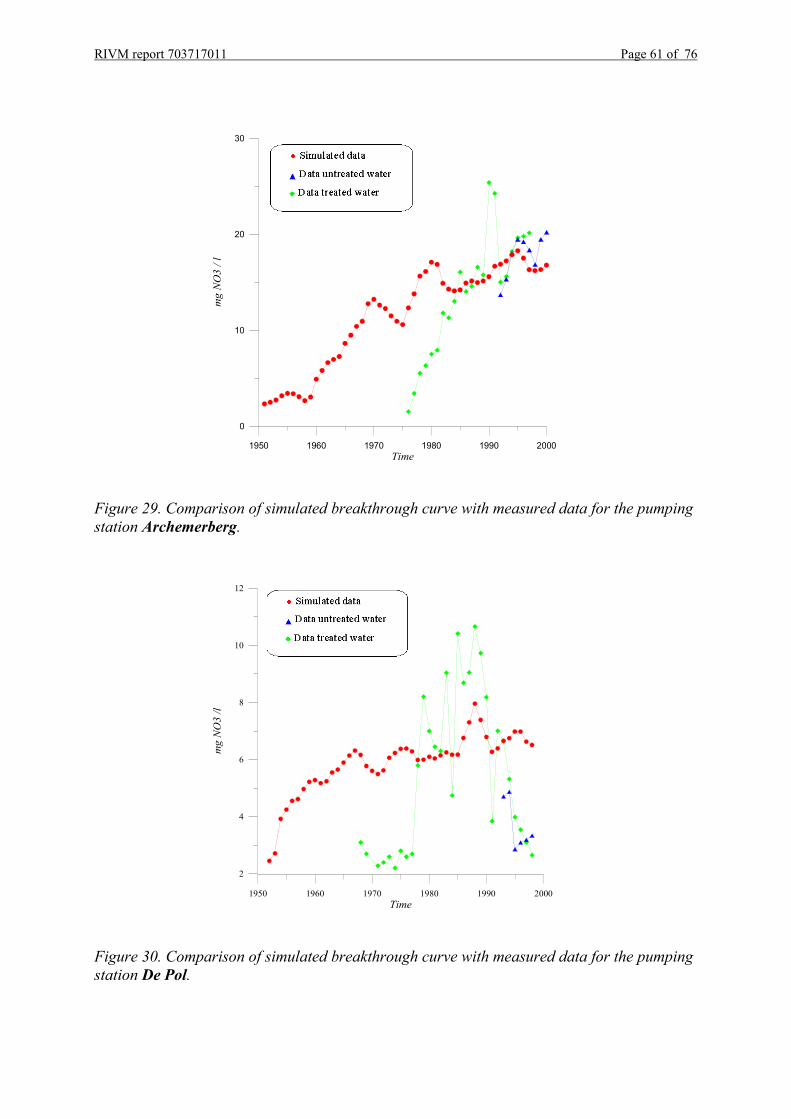
RIVM report 703717011 Page 61 of 76
Figure 29. Comparison of simulated breakthrough curve with measured data for the pumpingstation Archemerberg.
Figure 30. Comparison of simulated breakthrough curve with measured data for the pumpingstation De Pol.
1950 1960 1970 1980 1990 2000Time
0
10
20
30
mg
NO
3 / l
1950 1960 1970 1980 1990 2000Time
2
4
6
8
10
12
mg
NO
3 /l

Page 62 of 76 RIVM report 703717011
Figure 31. Comparison of simulated breakthrough curve with measured data for the pumpingstation Putten.
Figure 32. Measured data versus model results for the pumping station Putten.
1960 1970 1980 1990 2000Time
0
10
20
30
mg
NO
3 /l
-4 0 4 8Calculated ln(c)
-4
0
4
8
Mea
sure
d ln
(c)
Concentrations in mg NO3/l
Monitor Data
Breakthrough Data
Residual

RIVM report 703717011 Page 63 of 76
Figure 33. Comparison of simulated breakthrough curve with measured data for the pumpingstation Coevorden.
1950 1960 1970 1980 1990 2000Time
0.0
0.5
1.0
1.5
2.0
2.5
mg
NO
3 /l

Page 64 of 76 RIVM report 703717011

RIVM report 703717011 Page 65 of 76
9 Summary and conclusions
In modelling groundwater nitrate transport, denitrification has to be taken into account. Forthe simulation of denitrification the proposed model concept consists of three separateprocesses acting at different time rates:i) an instantaneous denitrification acting at or near the phreatic surface,ii) a relatively fast exponential decay that takes place in a zone where organic matter is likely
to be present,iii) a relative slow exponential decay in zones where organic material is absent.
The pilot study described in this report concerns the development and testing of a calibrationprocedure to estimate and optimise the parameter values of these three types of denitrification.The calibration itself has been carried out with a model-independent programme PEST.During calibration, model outcomes are matched with measured data. The data used formatching are nitrate concentrations observed in monitoring wells (LMG and PMG MonitoringNetworks), nitrate concentrations measured in the raw abstracted water as well as in thetreated water of several public water supply pumping stations. The nine selected pumpingstations are located in the central and eastern part of the Netherlands where highly permeablephreatic aquifers exist.
Nitrate measurements from the monitoring wells are representative for a small spatial area anda small time period. In practice these data can be considered as point measurements. Datataken from the water abstracted at the pumping stations represent a much larger area. Inhorizontal direction it corresponds to the capture zone of the pumping station. Nitratemeasurements of the abstracted water (breakthrough data) are collected since 1992 by theREWAB measuring programme. The REWAB data refer to water samples taken before thepurification process (untreated water) as well to samples from the purified water. Earlier dataexist from water samples taken after treatment (LMD measurement programme). During thepurification process no specific treatment is used for denitrification. In some cases nitratecontents before and after treatment are essentially the same. However, in other cases (e.g. atHerikerberg) a considerable difference is observed.
Nitrate transport modelling can not be carried out without information on the amount ofnitrate entering the aquifer system at the phreatic surface. Actual values for this nitrate fluxare not available. The present study uses nitrate fluxes that have been generated by theleaching model STONE. However, the STONE model concept differs from that of thegroundwater model, both temporally and in space. Therefore, several simplifying assumptionswere needed to transform nitrate fluxes from STONE to the format required for thegroundwater transport model. Another important simplification is related to the groundwaterflow. The groundwater flow has been treated as a steady state system. However, it is known,
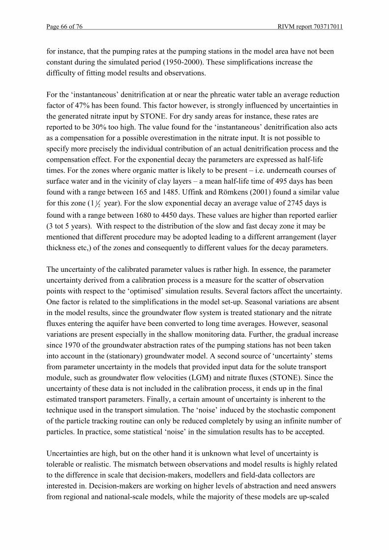
Page 66 of 76 RIVM report 703717011
for instance, that the pumping rates at the pumping stations in the model area have not beenconstant during the simulated period (1950-2000). These simplifications increase thedifficulty of fitting model results and observations.
For the ‘instantaneous’ denitrification at or near the phreatic water table an average reductionfactor of 47% has been found. This factor however, is strongly influenced by uncertainties inthe generated nitrate input by STONE. For dry sandy areas for instance, these rates arereported to be 30% too high. The value found for the ‘instantaneous’ denitrification also actsas a compensation for a possible overestimation in the nitrate input. It is not possible tospecify more precisely the individual contribution of an actual denitrification process and thecompensation effect. For the exponential decay the parameters are expressed as half-lifetimes. For the zones where organic matter is likely to be present – i.e. underneath courses ofsurface water and in the vicinity of clay layers – a mean half-life time of 495 days has beenfound with a range between 165 and 1485. Uffink and Römkens (2001) found a similar valuefor this zone ( 1
21 year). For the slow exponential decay an average value of 2745 days isfound with a range between 1680 to 4450 days. These values are higher than reported earlier(3 tot 5 years). With respect to the distribution of the slow and fast decay zone it may bementioned that different procedure may be adopted leading to a different arrangement (layerthickness etc,) of the zones and consequently to different values for the decay parameters.
The uncertainty of the calibrated parameter values is rather high. In essence, the parameteruncertainty derived from a calibration process is a measure for the scatter of observationpoints with respect to the ‘optimised’ simulation results. Several factors affect the uncertainty.One factor is related to the simplifications in the model set-up. Seasonal variations are absentin the model results, since the groundwater flow system is treated stationary and the nitratefluxes entering the aquifer have been converted to long time averages. However, seasonalvariations are present especially in the shallow monitoring data. Further, the gradual increasesince 1970 of the groundwater abstraction rates of the pumping stations has not been takeninto account in the (stationary) groundwater model. A second source of ‘uncertainty’ stemsfrom parameter uncertainty in the models that provided input data for the solute transportmodule, such as groundwater flow velocities (LGM) and nitrate fluxes (STONE). Since theuncertainty of these data is not included in the calibration process, it ends up in the finalestimated transport parameters. Finally, a certain amount of uncertainty is inherent to thetechnique used in the transport simulation. The ‘noise’ induced by the stochastic componentof the particle tracking routine can only be reduced completely by using an infinite number ofparticles. In practice, some statistical ‘noise’ in the simulation results has to be accepted.
Uncertainties are high, but on the other hand it is unknown what level of uncertainty istolerable or realistic. The mismatch between observations and model results is highly relatedto the difference in scale that decision-makers, modellers and field-data collectors areinterested in. Decision-makers are working on higher levels of abstraction and need answersfrom regional and national-scale models, while the majority of these models are up-scaled

RIVM report 703717011 Page 67 of 76
models that have been designed originally for the local scale. The up-scaling procedurerequires simplifications of the physical reality of the spatial and temporal variability.Obviously, we may not expect that these models produce accurate predictions for a certaintime at a certain location in 3D space. Nevertheless, this is exactly what is expected whenresults from larger scale models are compared with local scale measurements. At present aframework that allows us to transform raw measured data into figures that are more in linewith the model scale is not available. A future parameterisation and calibration of the modelmust rely on data derived from a statistical analysis that gives information on therepresentativeness of the measured data with respect to the model scale.
A more general aspect which is related to the above is the following. For long termpredictions and management evaluations on a regional scale usually highly up-scaled modelsare applied. Generally, however, for calibration of these models only data from small scaleand short term processes are available. This inconsistency between the scale of observationsand the resolution of the simulated data often prohibits a meaningful comparison of modeloutcomes and observations.
Calibration does not always lead to a unique set of parameter values. Difficulties with thisnon-uniqueness can be solved by application of a step-wise calibration procedure. In eachseparate step only one or a few selected parameter(s) are allowed to vary, while only thosemeasurements are selected that are the most sensitive to the ‘free’ parameter(s). The selectioncan be carried out at best by a sensitivity analysis. However, sensitivity analysis was notpossible with the version of PEST used in this study. A sensitivity analysis is highlyrecommended for future calibration exercises.
Finally a general remark must be made. From a groundwater quality point of view theoccurrence of denitrification is always regarded as a blessing. Indeed, it helps to remove anexcess of nitrate in groundwater. So far however, little attention is paid to the adverse effectsof denitrification. For instance, it is unknown whether the denitrification capacity of theunderground is unlimited or not. If the denitrification capacity gradually diminishes and theprocess is irreversible, it is a serious concern from the point of sustainable groundwatermanagement, especially as it is not known how fast this damage may develop. In the case ofdenitrification by pyrite-oxidation, trace elements (e.g. nickel, arsenic, zinc, and cadmium)dissolve in the groundwater, while it leads oxidation of sulphides to sulphates and mayincrease the water hardness. Another harmful aspect is the production of N2O as one of thefinal products of the denitrification process (Ronen et al., 1988). This gas is known as apotential destructor of the ozone layer and as a contributor to the ‘greenhouse’ effect.
The study described in this report demonstrates that for a stable groundwater transport modelcan be set-up for nitrates using a mixed zero and first order process to describe denitrification.Spatial variation of the denitrification parameters is possible by application of a zonation

Page 68 of 76 RIVM report 703717011
approach. Calibration of the model parameter is possible using nitrate measurements atmonitor wells and nitrate breakthrough curves at groundwater abstraction wells.

RIVM report 703717011 Page 69 of 76
Acknowledgements
Hereby, I would like to acknowledge my colleagues Karel Kovar and Jan Mülschlegel. Theircomments and fruitful suggestions have been of high value. Further, I would like to thank mycolleagues Rien Pastoors for providing the groundwater flow data (LGM), and Kees Schottenfor preparation of the data from the leaching model (STONE).

Page 70 of 76 RIVM report 703717011

RIVM report 703717011 Page 71 of 76
References
ANONYMOUS, 1993, Nagrom, Deelrapport 3, Supraregio Oost-Nederland, TNO-NITG,Rijkswaterstaat, RIZA. (In Dutch)
ANONYMOUS. 1994. Pest. Model independent parameter estimation. Watermark Computing(Available at http://www.sspa.com/pest/ 15 september 2003).
BEKINS, B.A. WARREN, E., GODSY, E.M. 1998. A comparison of zero-order, first-order andMonod biotransformation. Groundwater 36 (2): 261-268.
BEUSEN, A.H.W., BOOGAARD, H.L., FINKE, P.A., HEIDA, R., GEHRELS, B., GROENENDIJK,J.A., VAN JAARSVELD, J.A., KNOL, O.M., OVERBEEK, G.B.J., SCHEPER, E. 2000.STONE 1.3. Technische documentatie, Versie 1.0.
BOUMANS, L.J.M., VAN DRECHT, G. 1998. (In Dutch) Nitrate in the shallow groundwater inthe sandy areas of the Netherlands. A geographical description based on monitoring-dataand comparison with model results. RIVM report 714801015, Bilthoven.
COOLEY, R.L. 1983. Some procedures for numerical solution of variably saturated flowproblems. Water Resources Research, 19 (5), 1271-1285.
DOHERTY, J., JOHNSTON, J. M. 2003. Methodologies for calibration and predictive analysis ofa watershed model, J. American Water Resources Association, 39(2): 251-265.
GROOTJANS, P. 1984. De geohydrologische beschrijving van de provincie Gelderland. DienstGrondwaterverkenning TNO.
HAAG, D., KAUPENJOHANN, M. 2001. Landscape fate of nitrate fluxes and emissions inCentral Europe. A critical review of concepts, data, and models for transport andretention. Agriculture, Ecosystems and Environment 86, 1-21.
HILL, M.C. 1992. A Computer Program (MODFLOWP) for Estimating Parameters of atransient, Three-Dimensional, groundwater flow model using nonlinear regression. U.S.Geological Survey.
HISCOCK, K.M., LLOYD, J.W., LERNER, D.N. 1991. Review of natural and artificialdenitrification of groundwater. Water Research. 25 (9): 1099-1111.
KINZELBACH, W., UFFINK, G.J.M. 1991. The random walk method and extensions ingroundwater. In: Transport Processes in Porous Media (ed. By M. Corapcioglu), NATOASI Series, Serie C: Math. and Phys. Sci.
KÖLLE, W., WERNER, P., STREBEL, O., BÖTTCHER, J. 1985. Formation of sulphate bymicrobial denitrification in a reducing aquifer. Water Supply, 3 (1): 35-40.
KOROM, S.F. 1992. Natural denitrification in the saturated zone: A review, Water ResourcesResearch, 28(6), 1657-1668.
KOVAR, K., LEIJNSE, A., GAN, J.B.S. 1992. Groundwater Model for the Netherlands.Mathematical Model Development and User's Guide. RIVM Report 714305002, Bilthoven.
KOVAR, K., UFFINK, G.J.M., PASTOORS, M.J.H. 1996. Evaluation of the LGM GroundwaterModel the Netherlands for calculation of pathlines, travel times and concentration atabstraction wells. RIVM Report 703717001, Bilthoven.
KOVAR, K., PASTOORS, M.J.H., TIKTAK, A., VAN GAALEN, F.W. 1998. Application of theNetherlands Groundwater Model, LGM, for calculating concentration of nitrate andpesticides at abstraction wells in sandy soil areas of the Netherlands. RIVM Report703717002, Bilthoven.
LAWRENCE, A.R., FOSTER, S.S.D. 1986. Denitrification in a limestone aquifer in relation tothe security of low-nitrate supplies. J. Inst. Wat. Engng. Sci. 40, 159-172.
Page 72 of 76 RIVM report 703717011
LEIJNSE, A., PASTOORS, M.J.H. 1996. Calibration of the RIVM large-scale groundwater flowmodel (LGM for the Netherlands. In: Calibration and Reliability in GroundwaterModelling. Proc. ModelCARE 96 Conference. pp. 147-156.
MARIOTTI, A. 1986. La dénitrification dans les eaux souterraines, principes et méthodes deson identification: une revue. Journal of Hydrology, 80: 1-23.
MEINARDI, C.R. 1999. Personal Communication.OBERMANN, P. 1982. Contamination of groundwater in the lower Rhine region due to
agricultural activities on groundwater. In: Proceedings of the International Symposium onthe Impact of Agricultural Activities on Groundwater. Prague, pp. 285-297.
OVERBEEK, G.B.J., TIKTAK. A., BEUSEN, A.H.W., VAN PUIJENBROEK, P.J.T.M. 2001a. PartialValidation of the Dutch model for emission and transport of nutrients (STONE). Proc. 2nd
International Nitrogen Conference on Science and Policy. The ScientificWorld, P.M.2001.
OVERBEEK, G.B.J., VAN GRINSVEN, J.J.M., ROELSMA, J., GROENENDIJK, P., VAN EGMOND,P.M. BEUSEN, A.H.W. 2001b. Achtergronden bij de berekeningen van vermesting vanbodem en grondwater voor de 5e Milieuverkenning met het model STONE. RIVMrapport 408129020, Bilthoven.
PASTOORS, M.J.H. 1992. (In Dutch) National Groundwater Model; description of modelconcept. RIVM Report 714305004, Bilthoven.
RIVM, 2000. (In Dutch) National Environmental Outlook 5. 2000-2030. RIVM, Bilthoven.RONEN, D., MAGARITZ, M., ALMAN, E. 1988. Contaminated aquifers are a forgotten
component of the global N2O budget. Nature 335. 57-59.SNELTING, H., DE BOER, J.L.M., GAST, L.F.L., KUSSE, A.A.M., WILLEMSEN, W.H. 1990. (In
Dutch) Design and exploitation of the National Monitoring Network GroundwaterQuality. RIVM Report 728517061, Bilthoven.
STRACK, O.D.L. 1984. Three-dimensional streamlines in Dupuit-Forchheimer models. WaterResour. Res. 20 (7): 812-822.
TRUDELL, M.R., GILLHAM, R.W., CHERRY, J.A. 1986. An in-situ study of the occurrence andrate of denitrification in a shallow unconfined sand aquifer. Journ. of Hydrology. 83: 251-268.
UFFINK, G.J.M. 1990. Analysis of dispersion by the random walk method. Ph. D. Thesis.Delft University of Technology.
UFFINK, G.J.M. 1996. (In Dutch) National Groundwater Model (LGM). Test calculationsusing a solute transport module. RIVM Report. 715501008. Bilthoven.
UFFINK, G.J.M. 1999. LGMCAD, a solute transport module of the Groundwater Model forthe Netherlands. User’s Manual. RIVM Report 711401006, Bilthoven.
UFFINK, G.J.M., RÖMKENS, P.F.A.M. 2001. Nitrate transport modeling in deep aquifers.Comparison between model results and data from the Groundwater Monitoring Network.RIVM report 711401010, Bilthoven.
UFFINK, G.J.M. 2001. Modelling nitrate transport in deep aquifers. Comparison betweenmodel results and field-measurements. In: Impact of Human Activity on GroundwaterDynamics. Gehrels et al. (Eds). IAHS Publication 269. pp 339-341.
UFFINK, G.J.M., MÜLSCHLEGEL, J.H.C. 2002. (In Dutch) Application of LGMCAD for thecalculation of nitrates in abstracted groundwater at pumping stations in Twente and theAchterhoek. Also background document for the National Environmental Outlook 2000-2030. RIVM report 703717010, Bilthoven.
VAN BEEK, C.G.E.M., LAEVEN, M.P., VOGELAAR, A.J. 1994. (In Dutch) Modelleringdenitrificatie in grondwater onder invloed van organisch materiaal. H2O (27) nr 7: 180-184.

RIVM report 703717011 Page 73 of 76
VAN DRECHT, G., GOOSSENS, F.R., HACK-TEN-BROEKE, M.J.D., JANSEN, E.J.,STEENVOORDEN, J.H.A.M. 1991. (in Dutch) Berekening van de nitraatuitspoeling naar hetgrondwater met behulp van eenvoudige modellen. RIVM Report 724901003, Bilthoven.
VAN DRECHT, G. 1993. Modeling of regional scale nitrate leaching from agricultural soils, theNetherlands. Applied Geochemistry, Suppl. Issue 2, 175-178.
VAN DRECHT, G., SCHEPER, E. 1998. (in Dutch) Actualisering van model NLOAD voornitraatuitspoeling van landbouwgronden; beschrijving van model en GIS-omgeving.RIVM Report 711501002, Bilthoven.
VERMEULEN, P.T.M., STUURMAN, R.J., WITTE, J.PH.M., VAN DER MEIJDEN, R., GROEN,C.L.G. 1996. (In Dutch) Landelijke Hydrologische Systeemanalyse. Deelrapport 6. Hetgebied ten oosten van de IJssel (Salland, etc.). TNO-Report GG-R-95-91 (B).
WENDLAND, F. 1992. Die Nitratbelastung in den Grundwasserlandschaften der ‘alten’Bundesländer (BRD). Berichte aus der Ökologische Forschung. Band 8.
WENDLAND, F. 1994. Modelling the nitrate flow in groundwater provinces of the old federalstates of the Federal Republic of Germany. Ecol. Model. 757 (6), 385-397.

Page 74 of 76 RIVM report 703717011

RIVM report 703717011 Page 75 of 76
Mailing List
1 Drs. H.G. von Meijenfeldt, Ministerie VROM2 Ir. G.W. Ardon, Ministerie VROM3 Ir. W. Cramer, Ministerie VROM4 Prof. Dr. Ir. C. van den Akker, Technische Universiteit, Delft5 Dr. P.J.T. van Bakel, Alterra, Wageningen6 Dr. O. Batelaan, Vrije Universiteit Brussel, België7 Ir. C.G.E.M. van Beek, Kiwa, Nieuwegein8 Ir. H. Boukes, Adviesburo Harry Boukes, De Meern9 Ir. C. van den Brink, Royal Haskoning, Groningen10 Drs. H.P. Broers, Universiteit Utrecht11 Ir. J. Griffioen, NITG-TNO, Utrecht12 Drs. G.J.W. Krajenbrink, Waterleiding Laboratorium Oost, Doetinchem13 Dr. Ir. W. de Lange, RIZA, Lelystad14 Prof. Dr. Ir. A. Leijnse, NITG-TNO, Utrecht15 Drs. G.B.J. Overbeek, Tebodin, Hengelo16 Dr. Ir. P.F.A.M. Römkens, Alterra, Wageningen17 Dr. Ir. P. Venema, NITG-TNO, Delft18 Dr. K. Walraevens, Universiteit van Gent, België19 Dr. Ir. W.J. Zaadnoordijk, Royal Haskoning, Rotterdam20-29 Werkgroep Pyriet, p/a mw H. de Ruiter WMO30 Bibliotheek VEWIN31 Bibliotheek KIWA32 Prof. Ir. N.D. Van Egmond33 Ir. F. Langeweg34 Ir. R. van den Berg35 Drs. A.H.W. Beusen36 Ir. L.J.M. Boumans37 Dr. Ir. J.J.B. Bronswijk38 Drs. J.H. Canton39 Ir. G. van Drecht40 Dr. Ir. J.J.M. van Grinsven41 Ir. B.J. de Haan42 Ir. J.J.G. Kliest43 Ir. K. Kovar44 Ir. J.H.C. Mülschlegel

Page 76 of 76 RIVM report 703717011
45 Ir. M.J.H. Pastoors46 Dr. H.F.R. Reijnders47 Ir. C.G.J. Schotten48 Dr. A. Tiktak49 Ir. J.F.M. Versteegh50 Drs. W.J. Willems51 Dr. Ir. R.D. Woittiez52 Depôt Nederlandse Publikaties en Nederlands Bibliografie53-54 Auteur55 Bureau Rapportenregistratie56 SBC/afd. Communicatie57 Bibliotheek RIVM58-62 Bureau Rapportenbeheer63-78 Reserve exemplaren