A particle swarm pattern search method for

bound constrained global optimization

A. Ismael F. Vaz ∗ L. N. Vicente †

December 21, 2006

Abstract

In this paper we develop, analyze, and test a new algorithm for theglobal minimization of a function subject to simple bounds withoutthe use of derivatives. The underlying algorithm is a pattern searchmethod, more specifically a coordinate search method, which guaran-tees convergence to stationary points from arbitrary starting points.

In the optional search phase of pattern search we apply a par-ticle swarm scheme to globally explore the possible nonconvexity ofthe objective function. Our extensive numerical experiments showedthat the resulting algorithm is highly competitive with other globaloptimization methods also based on function values.

Keywords: Direct search, pattern search, particle swarm, derivative freeoptimization, global optimization, bound constrained nonlinear optimization.

AMS subject classifications: 90C26, 90C30, 90C56.

1 Introduction

Pattern and direct search methods are one of the most popular classes ofmethods to minimize functions without the use of derivatives or of approxi-mations to derivatives [26]. They are based on generating search directions

∗Departamento de Producao e Sistemas, Escola de Engenharia, Universidade do Minho,Campus de Gualtar, 4710-057 Braga, Portugal (aivaz@dps.uminho.pt). Support forthis author was provided by Algoritmi Research Center, and by FCT under grantsPOCI/MAT/59442/2004 and POCI/MAT/58957/2004.

†Departamento de Matematica, Universidade de Coimbra, 3001-454 Coimbra, Portugal(lnv@mat.uc.pt). Support for this author was provided by Centro de Matematica daUniversidade de Coimbra and by FCT under grant POCI/MAT/59442/2004.

1

which positively span the search space. Direct search is conceptually simpleand natural for parallelization. These methods can be designed to rigorouslyidentify points satisfying stationarity for local minimization (from arbitrarystarting points). Moreover, their flexibility can be used to incorporate al-gorithms or heuristics for global optimization, in a way that the resultingdirect or pattern search method inherits some of the properties of the im-ported global optimization technique, without jeopardizing the convergencefor local stationarity mentioned before.

The particle swarm optimization algorithm was firstly proposed in [11, 24]and has received some recent attention in the global optimization commu-nity [12, 35]. The particle swarm algorithm tries to simulate the social be-haviour of a population of agents or particles, in an attempt to optimallyexplore some given problem space. At a time instant (an iteration in theoptimization context), each particle is associated with a stochastic velocityvector which indicates where the particle is moving to. The velocity vectorfor a given particle at a given time is a linear stochastic combination of thevelocity in the previous time instant, of the direction to the particle’s bestposition, and of the direction to the best swarm positions (for all particles).The particle swarm algorithm is a stochastic algorithm in the sense that itrelies on parameters drawn from random variables, and thus different runsfor the same starting swarm may produce different outputs. Some of its ad-vantages are being simple to implement and easy to parallelize. It depends,however, on a few of parameters which influence the rate of convergence in thevicinity of the global optimum. Overall it does not require many user-definedparameters, which is important for practitioners that are not familiar withoptimization. Some numerical evidence seems to show that particle swarmcan outperform genetic algorithms on difficult problem classes, namely forunconstrained global optimization problems [6]. Moreover, it fits nicely intothe pattern search framework.

The goal of this paper is to show how particle swarm can be incorporatedin the pattern search framework. The resulting particle swarm pattern searchalgorithm is still a pattern search algorithm, producing sequences of iteratesalong the traditional requirements for this class of methods (based on integerlattices and positive spanning sets). The new algorithm is better equippedfor global optimization because it is more aggressive in the exploration of thesearch space. Our numerical experiences showed that a large percentage ofthe computational work is spent in the particle swarm component of patternsearch.

Within the pattern search framework, the use of the search step for sur-rogate optimization [5, 30] or global optimization [1] is an active area ofresearch. Hart has also used evolutionary programming to design evolution-

2

ary pattern search methods (see [16] and the references therein). There aresome significative differences between his work and ours. First, we are exclu-sively focused on global optimization and our heuristic is based on particleswarm rather than on evolutionary algorithms. Further, our algorithm isdeterministic in its pattern search component. As a result, we obtain that asubsequence of the mesh size parameters tends to zero is the deterministicsense rather than with probability one like in Hart’s algorithms.

We are interested in solving mathematical problems of the form

minz∈Rn

f(z) s.t. z ∈ Ω,

withΩ = z ∈ R

n : ℓ ≤ z ≤ u ,

where the inequalities ℓ ≤ z ≤ u are posed componentwise and ℓ ∈ (−∞, R)n,u ∈ (R, +∞, )n, and ℓ < u. There is no need to assume any type on smooth-ness on the objective function f(z) to apply particle swarm or pattern search.To study the convergence properties of pattern search, and thus of the par-ticle swarm pattern search method, one has to impose some smoothness onf(z), in particular to characterize stationarity at local minimizers.

The next two sections are used to describe the particle swarm paradigmand the basic pattern search framework. We introduce the particle swarmpattern search method in Section 4. The convergence and termination prop-erties of the proposed method are discussed in Section 5. A brief reviewabout the optimization solvers used in the numerical comparisons and im-plementation details about our method are given in Section 6. The numericalresults are presented in Section 7 for a large set of problems. We end thepaper in Section 8 with conclusions and directions for future work.

2 Particle swarm

In this section, we briefly describe the particle swarm optimization algorithm.Our description follows the presentation of the algorithm tested in [6] andthe reader is pointed to [6] for other algorithmic variants and details.

The particle swarm optimization algorithm is based on a population(swarm) of s particles, where s is known as the population size. Each particleis associated with a velocity which indicates where the particle is moving to.Let t be a time instant. The new position xi(t + 1) of the i–th particle attime t+1 is computed by adding to the old position xi(t) at time t a velocityvector vi(t + 1):

xi(t + 1) = xi(t) + vi(t + 1), (1)

3

for i = 1, . . . , s.The velocity vector associated to each particle i is updated by

vij(t + 1) = ι(t)vi

j(t) + µω1j(t)(

yij(t) − xi

j(t))

+ νω2j(t)(

yj(t) − xij(t)

)

, (2)

for j = 1, . . . , n, where ι(t) is a weighting factor (called inertial) and µ andν are positive real parameters (called, in the particle swarm terminology, thecognition parameter and the social parameter, respectively). The numbersω1j(t) and ω2j(t), j = 1, . . . , n, are randomly drawn from the uniform (0, 1)distribution. Finally, yi(t) is the position of the i-th particle with the bestobjective function value so far calculated, and y(t) is the particle positionwith the best (among all particles) objective function value found so far.The update formula (2) adds to the previous velocity vector a stochasticcombination of the directions to the best position of the i-th particle and tothe best (among all) particles position.

The position y(t) can be described as

y(t) ∈ argminz∈y1(t),...,ys(t)f(z).

The argmin operator can return a set. When that happens in this situation,it is the first element in this argmin set that matches the implementations,since the best element is only updated algorithmically when a new one isfound yielding a decrease in the objective function.

The bound constraints in the variables are enforced by considering theprojection onto Ω, given for all particles i = 1, . . . , s by

projΩ(xij(t)) =

ℓj if xij(t) < ℓj ,

uj if xij(t) > uj,

xij(t) otherwise,

(3)

for j = 1, . . . , n. This projection must be applied to the new particles posi-tions computed by equation (1).

The stopping criterion of the algorithm should be practical and has toensure proper termination. One possibility is to stop when the norm of thevelocities vector is small for all particles. It is possible to prove under someassumptions and for some algorithmic parameters that the expected value ofthe norm of the velocities vectors tends to zero for all particles (see also theanalysis presented in Section 5).

The particle swarm optimization algorithm is described in Algorithm 2.1.

4

Algorithm 2.1

1. Choose a population size s and a stopping tolerance vtol > 0. Ran-domly initialize the initial swarm positions x1(0), . . . , xs(0) and the ini-tial swarm velocities v1(0), . . . , vs(0).

2. Set yi(0) = xi(0), i = 1, . . . , s, and y(0) ∈ arg minz∈y1(0),...,ys(0) f(z).Let t = 0.

3. Set y(t + 1) = y(t).

For i = 1, . . . , s do (for every particle i):

• Compute xi(t) = projΩ(xi(t)).

• If f(xi(t)) < f(yi(t)) then

– Set yi(t + 1) = xi(t) (update the particle i best position).

– If f(yi(t + 1)) < f(y(t + 1)) then y(t + 1) = yi(t + 1) (updatethe particles best position).

• Otherwise set yi(t + 1) = yi(t).

4. Compute vi(t+1) and xi(t+1), i = 1, . . . , s, using formulae (1) and (2).

5. If ‖vi(t+1)‖ < vtol, for all i = 1, . . . , s, then stop. Otherwise, incrementt by one and go to Step 3.

3 Pattern search

Direct search methods are an important class of optimization algorithmswhich attempt to minimize a function by comparing, at each iteration, itsvalue in a finite set of trial points (computed by simple mechanisms). Directsearch methods not only do not use any derivative information but also donot try to implicitly build any type of derivative approximation. Patternsearch methods can be seen as direct search methods for which the rulesof generating the trial points follow stricter calculations and for which con-vergence for stationary points can be proved from arbitrary starting points.A comprehensive review of direct and pattern search can be found in [26],where a broader class of methods referred to as ’generating set search’ isdescribed. In this paper, we prefer to describe pattern search methods usingthe search/poll step framework [3], since it better suits the incorporation ofheuristic procedures.

The central notion in pattern search are positive spanning sets. Thedefinitions and properties of positive spanning sets and of positive bases are

5

given, for instance, in [9, 26]. One of the simplest positive spanning sets isformed by the vectors of the canonical basis and their negatives:

D⊕ = e1, . . . , en,−e1, . . . ,−en.

The set D⊕ is also a (maximal) positive basis. The elementary direct searchmethod based on this positive spanning set is known as coordinate or compasssearch and its structure is basically all we need in this paper.

Given a positive spanning set D and the current iterate1 y(t), we definetwo sets of points: the mesh Mt and the poll set Pt. The mesh Mt is givenby

Mt =

y(t) + α(t)Dz, z ∈ Z|D|+

,

where α(t) > 0 is the mesh size parameter (also known as the step-lengthcontrol parameter) and Z+ is the set of nonnegative integers. The meshhas to meet some integrality requirements for the method to achieve globalconvergence to stationary points, in other words, convergence to stationarypoints from arbitrary starting points. In particular, the matrix D has to beof the form GZ, where G ∈ R

n×n is a nonsingular generating matrix andZ ∈ Z

n×|D|. The positive basis D⊕ satisfies this requirement trivially whenG is the identity matrix.

The search step conducts a finite search in the mesh Mt. The poll step isexecuted only if the search step fails to find a point for which f is lower thanf(y(t)). The poll step evaluates the function at the points in the poll set

Pt = y(t) + α(t)d, d ∈ D ,

trying to find a point where f is lower than f(y(t)). Note that Pt is a subsetof Mt. If f is continuously differentiable at y(t), the poll step is guaranteedto succeed if α(t) is sufficiently small, since the positive spanning set Dcontains at least one direction of descent (which makes an acute angle with−∇f(y(t))). Thus, if the poll step fails then the mesh size parameter mustbe reduced. It is the poll step that guarantees the global convergence of thepattern search method.

In order to generalize pattern search for bound constrained problems itis necessary to use a feasible initial guess y(0) ∈ Ω and to keep feasibilityof the iterates by rejecting any trial point that is out of the feasible region.Rejecting infeasible trial points can be accomplished by applying a patternsearch algorithm to the following penalty function

f(z) =

f(z) if z ∈ Ω,+∞ otherwise.

1We will use y(t) to denote the current iterate, rather than xk or yk, to follow thenotation of the particle swarm framework.

6

The iterates produced by a pattern search method applied to the uncon-strained problem of minimizing f(z) coincide trivially with those generatedby the same type of pattern search method, but applied to the minimizationof f(z) subject to simple bounds and to the rejection of infeasible trial points.

It is also necessary to include in the search directions D those directionsthat guarantee the presence of a feasible descent direction at any nonstation-ary point of the bound constrained problem. One can achieve this goal inseveral ways. But, since D⊕ includes all such directions [26], we assume theuse of this set throughout the remainder of the paper.

In order to completely describe the basic pattern search algorithm, weneed to specify how to expand and contract the mesh size or step-lengthcontrol parameter α(t). These expansions and contractions use the factorsφ(t) and θ(t), respectively, which must obey to the following rules:

φ(t) = τ ℓt , for some ℓt ∈ 0, . . . , ℓmax, if t is successful,θ(t) = τmt , for some mt ∈ mmin, . . . ,−1, if t is unsuccessful,

where τ > 1 is a positive rational, ℓmax is a nonnegative integer, and mmin

is a negative integer, chosen at the beginning of the method and unchangedwith t. For instance, we can have θ(t) = 1/2 for unsuccessful iterations andφ(t) = 1 or φ(t) = 2 for successful iterations.

The basic pattern search method for use in this paper is described inAlgorithm 3.1.

Algorithm 3.1

1. Choose a positive rational τ and the stopping tolerance αtol > 0. Choosethe positive spanning set D = D⊕.

2. Let t = 0. Select an initial feasible guess y(0). Choose α(0) > 0.

3. [Search Step]

Evaluate f at a finite number of points in Mt. If a point z(t) ∈ Mt isfound for which f(z(t)) < f(y(t)) then set y(t + 1) = z(t), α(t + 1) =φ(t)α(t) (optionally expanding the mesh size parameter), and declaresuccessful both the search step and the current iteration.

4. [Poll Step]

Skip the poll step if the search step was successful.

• If there exists d(t) ∈ D such that f(y(t)+α(t)d(t)) < f(y(t)) then

7

– Set y(t + 1) = y(t) + α(t)d(t) (poll step and iteration success-ful).

– Set α(t + 1) = φ(t)α(t) (optionally expand the mesh size pa-rameter).

• Otherwise, f(y(t) + α(t)d(t)) ≥ f(y(t)) for all d(t) ∈ D, and

– Set y(t + 1) = y(t) (iteration and poll step unsuccessful).

– Set α(t + 1) = θ(t)α(t) (contract the mesh size parameter).

5. If α(t + 1) < αtol then stop. Otherwise, increment t by one and go toStep 3.

An example of the use of the search step is given in the next section. Thepoll step can be implemented in a number of different ways. The pollingcan be opportunistic (when it quits once the first decrease in the objectivefunction is found) or complete (when the objective function is evaluated at allthe points of the poll set). The order in which the points in Pt are evaluatedcan also differ [4, 8].

4 The particle swarm pattern search method

Pattern search methods are local methods in the sense that they are designedto achieve convergence (from arbitrary starting points) to points that satisfynecessary conditions for local optimality. Some numerical experience hasshown cases in which pattern search has found global minimizers for certainclasses of problems (see, for instance, [1, 31]). Certain parameter choicescan enable pattern search to jump out of one basin of attraction of a localminimizer into another (that is hopefully a better one). This paper is anattempt to exploit this tendency by applying a global heuristic in the searchstep. On the other hand, the poll step can rigorously guarantee convergenceto stationary points.

The hybrid method introduced in this paper is a pattern search methodthat incorporates a particle swarm search in the search step. The idea isto start with an initial population and to apply one step of particle swarmat each search step. Consecutive iterations where the search steps succeedreduce to consecutive iterations of particle swarm, in an attempt to identifya neighborhood of a global minimizer. Whenever the search step fails, thepoll step is applied to the best position over all particles, performing a localsearch in the poll set centered at this point.

The points calculated in the search step by the particle swarm schememust belong to the pattern search mesh Mt. This task can be done in several

8

ways and, in particular, one can compute their ‘projection’ onto Mt

projMt(xi(t)) = min

u∈Mt

‖u − xi(t)‖,

for i = 1, . . . , s, or an approximation thereof.There is no need then to project onto Ω since the use of the penalty

function f in pattern search takes care of the bound constraints.The stopping criterion of the particle swarm pattern search method is the

conjunction of the stopping criteria for particle swarm and pattern search.The particle swarm pattern search method is described in Algorithm 4.1.

Algorithm 4.1

1. Choose a positive rational τ and the stopping tolerance αtol > 0. Choosethe positive spanning set D = D⊕.

Choose a population size s and a stopping tolerance vtol > 0. Ran-domly initialize the initial swarm positions x1(0), . . . , xs(0) and the ini-tial swarm velocities v1(0), . . . , vs(0).

2. Set yi(0) = xi(0), i = 1, . . . , s, and y(0) ∈ arg minz∈y1(0),...,ys(0) f(z).Choose α(0) > 0. Let t = 0.

3. [Search Step]

Set y(t + 1) = y(t).

For i = 1, . . . , s do (for every particle i):

• Compute xi(t) = projMt(xi(t)).

• If f(xi(t)) < f(yi(t)) then

– Set yi(t + 1) = xi(t) (update the particle i best position).

– If f(yi(t + 1)) < f(y(t + 1)) then

∗ Set y(t+1) = yi(t+1) (update the particles best position;search step and iteration successful).

∗ Set α(t + 1) = φ(t)α(t) (optionally expand the mesh sizeparameter).

• Otherwise set yi(t + 1) = yi(t).

4. [Poll Step]

Skip the poll step if the search step was successful.

• If there exists d(t) ∈ D such that f(y(t)+α(t)d(t)) < f(y(t)) then

9

– Set y(t + 1) = y(t) + α(t)d(t) (update the leader particle posi-tion; poll step and iteration successful).

– Set α(t + 1) = φ(t)α(t) (optionally expand the mesh size pa-rameter).

• Otherwise, f(y(t) + α(t)d(t)) ≥ f(y(t)) for all d(t) ∈ D, and

– Set y(t + 1) = y(t) (no change in the leader particle position;poll step and iteration unsuccessful).

– Set α(t + 1) = θ(t)α(t) (contract the mesh size parameter).

5. Compute vi(t+1) and xi(t+1), i = 1, . . . , s, using formulae (1) and (2).

6. If α(t + 1) < αtol and ‖vi(t + 1)‖ < vtol, for all i = 1, . . . , s, then stop.Otherwise, increment t by one and go to Step 3.

5 Convergence

The convergence analysis studies properties of a sequence of iterates gener-ated by Algorithm 4.1. For this purpose, we consider αtol = 0 and vtol = 0, sothat the algorithm never meets the termination criterion. Let y(t) be thesequence of iterates produced by Algorithm 4.1. Since all necessary patternsearch ingredients are present, this method generates, under the appropriateassumptions, a sequence of iterates converging (independently of the startingpoint) to first-order critical points. A standard result for this class of meth-ods tells us that there is a subsequence of unsuccessful iterations convergingto a limit point and for which the mesh size parameter tends to zero [3, 26].

Theorem 5.1 Let L(y(0)) = z ∈ Rn : f(z) ≤ f(y(0)) be a bounded

set. Then, there exists a subsequence y(tk) of the iterates produced byAlgorithm 4.1 (with αtol = vtol = 0) such that

limk−→+∞

y(tk) = y∗ and limk−→+∞

α(tk) = 0,

for some y∗ ∈ Ω and such that the subsequence tk consists of unsuccessfuliterations.

The integrality assumptions imposed in the construction of the meshesMt and on the update of the mesh size parameter are fundamental for theinteger lattice type arguments required to prove this result. There are otherways to obtain such a result that circumvent the need for these integrality

10

assumptions [26], such as the imposition of a sufficient decrease condition onthe step acceptance mechanism of the poll step.

Depending on the differentiability properties of the objective function,different types of stationarity can be proved for the point y∗. For instance,if the function is strictly differentiable at this point, one can prove fromthe positive spanning properties of D that ∇f(y∗) = 0 (see [3]). A resultof the type lim inft−→+∞ ‖∇f(y(t))‖ = 0 can only be guaranteed when f iscontinuously differentiable in L(y(0)) (see [26]).

Theorem 5.1 tells us that a stopping criterion based solely on the size ofthe mesh size parameter (of the form α(t) < αtol) will guarantee terminationof the algorithm in a finite number of iterations. However, the stoppingcondition of Algorithm 4.1 also requires ‖vi(t)‖ < vtol, i = 1, . . . , s (in anattempt to impose to particle swarm a desirable level of global optimizationeffort). Thus, it must be investigated whether or not the velocities in theparticle swarm scheme satisfy a limit of the form

limk−→+∞

‖vi(tk)‖ = 0 i = 1, . . . , s.

To do this we have to investigate the asymptotic behavior of the search stepwhich is where the particle swarm strategy is applied. Rigorously speakingsuch a limit can only occur with probability one. To carry on the analysiswe need to assume that xi(t), yi(t), vi(t), and y(t) are random variables ofstochastic processes. Let E(·) denoted the appropriate mean or expectedvalue operator.

Theorem 5.2 Suppose that for t sufficiently large one has that ι(t), E(yi(t)),i = 1, . . . , s, and E(y(t)) are constant and that E(projMt

(xi(t−1)+vi(t))) =E(xi(t− 1) + vi(t)), i = 1, . . . , s. Then, if the control parameters for particleswarm, ι, ω1, ω2, µ, and ν, are chosen so that max|a|, |b| < 1, whereω1 = E(ω1(t)), ω2 = E(ω2(t)), ι = ι(t) for all t, and a and b are definedrespectively by (8) and (9), then

limt−→+∞

E(vij(t)) = 0, i = 1, . . . , s, j = 1, . . . , n.

and Algorithm 4.1 will stop almost surely in a finite number of iterations.

Proof. Given that there exists a subsequence driving the mesh size pa-rameter to zero, it remains to investigate under what conditions do the ve-locities tend to zero.

Consider the velocity equation (2), repeated here for convenience, withthe indices i for the particles and j for the vector components dropped for

11

simplicity. To shorten notation we write the indices t as subscripts. Sinceω1(t) and ω2(t) depend only on t, we get from (2) that

E(vt+1) = ιE(vt) + µω1 (E(yt) − E(xt)) + νω2 (E(yt) − E(xt)) . (4)

where ω1 = E(ω1(t)) and ω2 = E(ω2(t)). From (2), we obtain for v(t) that

E(vt) = ιE(vt−1) + µω1 (E(yt−1) − E(xt−1))

+ νω2 (E(yt−1) − E(xt−1)) . (5)

Subtracting (5) from (4) yields

E(vt+1) − E(vt) = ι(E(vt) − E(vt−1)) − (µω1 + νω2)(E(xt) − E(xt−1))

+ µω1(E(yt) − E(yt−1)) + νω2(E(yt) − E(yt−1)).

Noting that xt = projMt(xt−1+vt) we obtain the following inhomogeneous

recurrence relation

E(vt+1) − (1 + ι − µω1 − νω2)E(vt) + ιE(vt−1) = gt, (6)

where

gt = µω1(E(yt) − E(yt−1)) + νω2(E(yt) − E(yt−1))

+ (µω1 + νω2)E(projMt(xt−1 + vt) − (xt−1 + vt)).

From the assumptions of the theorem, we have, for sufficiently large t,that gt is zero and therefore that the recurrence relation is homogeneous,with characteristic polynomial given by

t2 − (1 + ι − µω1 − νω2)t + ι = 0. (7)

A solution of (6) is then of the form

E(vt+1) = c1at + c2b

t,

where c1 and c2 are constants and a and b are the two roots of the charac-teristic polynomial (7), given by

a =(1 + ι − µω1 − νω2) +

√

(1 + ι − µω1 − νω2)2 − 4ι

2, (8)

b =(1 + ι − µω1 − νω2) −

√

(1 + ι − µω1 − νω2)2 − 4ι

2. (9)

12

0 0.1 0.2 0.3 0.4 0.5 0.6 0.7 0.8 0.9 10

0.1

0.2

0.3

0.4

0.5

0.6

0.7

0.8

0.9

1

ι

|a|,|

b|

|b|

|a|

|a|,|b|

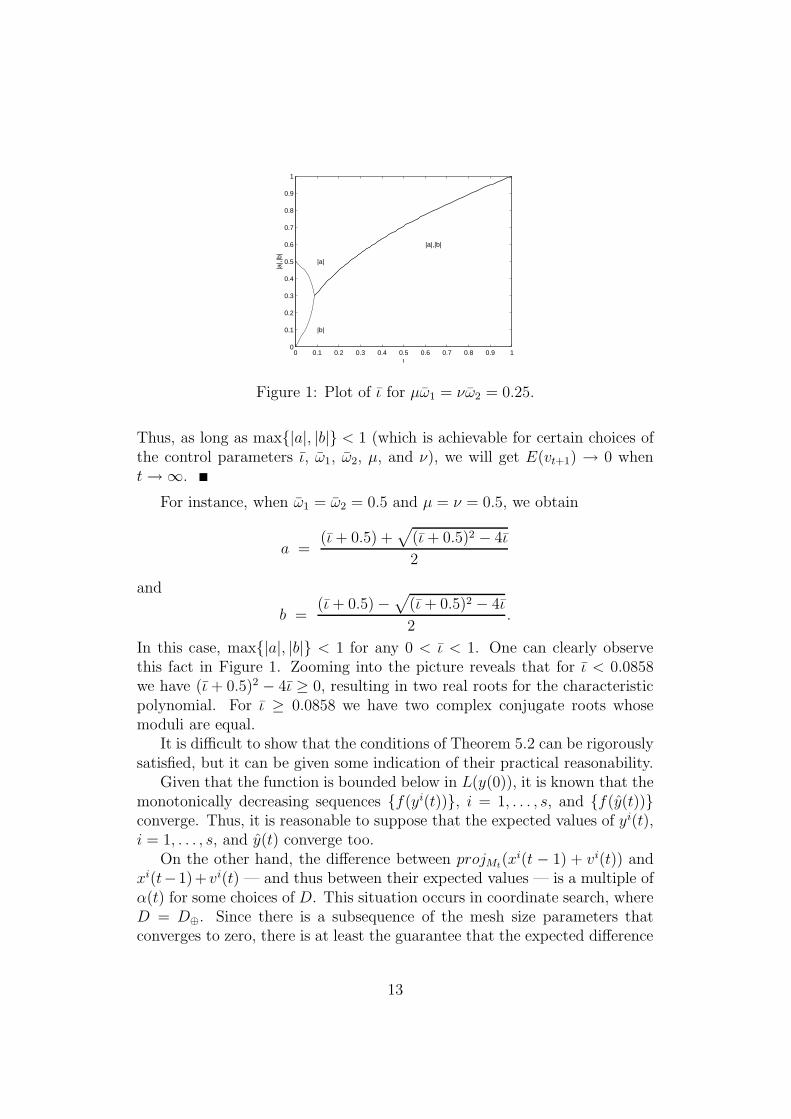
Figure 1: Plot of ι for µω1 = νω2 = 0.25.

Thus, as long as max|a|, |b| < 1 (which is achievable for certain choices ofthe control parameters ι, ω1, ω2, µ, and ν), we will get E(vt+1) → 0 whent → ∞.

For instance, when ω1 = ω2 = 0.5 and µ = ν = 0.5, we obtain

a =(ι + 0.5) +

√

(ι + 0.5)2 − 4ι

2

and

b =(ι + 0.5) −

√

(ι + 0.5)2 − 4ι

2.

In this case, max|a|, |b| < 1 for any 0 < ι < 1. One can clearly observethis fact in Figure 1. Zooming into the picture reveals that for ι < 0.0858we have (ι + 0.5)2 − 4ι ≥ 0, resulting in two real roots for the characteristicpolynomial. For ι ≥ 0.0858 we have two complex conjugate roots whosemoduli are equal.

It is difficult to show that the conditions of Theorem 5.2 can be rigorouslysatisfied, but it can be given some indication of their practical reasonability.

Given that the function is bounded below in L(y(0)), it is known that themonotonically decreasing sequences f(yi(t)), i = 1, . . . , s, and f(y(t))converge. Thus, it is reasonable to suppose that the expected values of yi(t),i = 1, . . . , s, and y(t) converge too.

On the other hand, the difference between projMt(xi(t − 1) + vi(t)) and

xi(t−1)+vi(t) — and thus between their expected values — is a multiple ofα(t) for some choices of D. This situation occurs in coordinate search, whereD = D⊕. Since there is a subsequence of the mesh size parameters thatconverges to zero, there is at least the guarantee that the expected difference

13

between xi(t−1)+ vi(t) and its projection onto Mt converges to zero in thatsubsequence.

So, there is at least some indication that the term gt in (6) convergesto zero for a subsequence of the iterates. Although this is not the same assaying that the assumptions of Theorem 5.2 are satisfied, it helps to explainthe observed numerical termination of the algorithm.

6 Optimization solvers used for comparison

The particle swarm pattern search algorithm (Algorithm 4.1) was imple-mented in the C programming language. The solver is referred to as PSwarm.

In order to assess the performance of PSwarm, a set of 122 global opti-mization test problems from the literature ([2, 17, 21, 25, 28, 29, 32, 34])was collected and coded in AMPL. See Table 2. All coded problems havelower and upper bounds on the variables. The problems description and theirsource are available at http://www.norg.uminho.pt/aivaz under software.

AMPL [14] is a mathematical modeling language which allows an easyand fast way to code optimization problems. AMPL provides also automaticdifferentiation (not used in the context of derivative free optimization) andinterfaces to a number of optimization solvers. The AMPL mechanism totune solvers was used to pass options to PSwarm.

6.1 Solvers

The optimization solver PSwarm was compared to a few solvers for globaloptimization, namely DIRECT [13], ASA [20], MCS [19], and PGAPack [27].

DIRECT is an implementation of the method described in [23]. DIRECT

reads from DIviding RECTangles and it is implemented in MATLAB. (Inour numerical tests we used MATLAB Version 6, Release 12.) DIRECT solvedthe problems coded in AMPL by using the amplfunc external AMPL func-tion [15] for MATLAB together with a developed M-file to interface DIRECT

with AMPL.ASA is an implementation in C of the Adaptative Simulated Annealing.

The user has to write its objective function as a C function and to compile itwith the optimization code. Options are defined during compilation time. Touse the AMPL coded problems, an interface for AMPL was also developed.Here, we have followed the ideas of the MATLAB interface to ASA providedby S. Sakata (see http://www.econ.lsa.umich.edu/∼sakata/software).

MCS stands for Multilevel Coordinate Search and it is inspired by themethods of Jones et al. [23]. MCS is implemented in MATLAB and, as with

14

DIRECT, the AMPL interface to MATLAB and a developed M-file were usedto obtain the numerical results for the AMPL coded problems.

PGAPack is an implementation of a genetic algorithm. The Parallel Ge-netic Algorithm Pack is written in C. As in ASA, the user defines a C functionand compiles it along with the optimization code. As for ASA, an interfaceto AMPL was also developed. The population size selected for PGAPAck waschanged to 200 (since it performed better with a higher population size).

DIRECT and MCS are deterministic codes. The other two, PGAPack and ASA,together with PSwarm, are stochastic ones. A relevant issue in stochastic codesis the choice of the underlying random number generator. It is well knownthat good random number generators are hard to find (see, for example, [33]).ASA and Pswarm use the number generator from [7, 33]. PGAPack uses agenerator described in [22].

6.2 PSwarm details

The default values for PSwarm are αtol = 10−5, ν = µ = 0.5, α(0) =maxj=1,..,n(uj − ℓj)/c with c = 5, and s = 20. The contraction of the meshsize parameter used θ(t) = 0.5. The expansion was only applied when twoconsecutive polls steps occured using the same polling direction [18]; in thesecases we set φ(t) = 2. Polling was implemented in the opportunistic way(accepting the first polling point that yielded decrease). The projection ontothe mesh (xi(t) = projMt

(xi(t))) has not been implemented in the searchstep.

The inertial parameter ι(t) is linearly interpolated between 0.9 and 0.4,i.e., ι(t) = 0.9−(0.5/tmax)t, where tmax is the maximum number of iterationspermitted. Larger values for max|a|, |b| will result in slower convergence.Thus, we start with a slower rate and terminate faster.

The initial swarm is obtained by generating s random feasible pointsuniformly distributed on (ℓ, u).

In particle swarm all particles will in principle converge to y, and a highconcentration of particles is needed in order to obtain a solution with somedegree of precision. Thus, in the last iterations of particle swarm, a highnumber of objective function evaluations is necessary to obtain some precisionin the solution. Removing particles from the swarm that are near othersseems like a good idea, but a price in precision is paid in order to gain adecrease in the number of objective function evaluations.

In the proposed particle swarm pattern search algorithm the scenario issomehow different since the y particle position is improved by the poll steps ofpattern search. Removing particles that do not drive the search to a globalminimizer is highly desirable. A particle i is removed from the swarm in

15

PSwarm when it is close to y, i.e., when ‖yi(t) − y(t)‖ ≤ α(0). If a particle isclose to y (compared in terms of α(0)) it means that it is unlikely to furtherexplore the search space for a global optimum.

6.3 Performance profiles

A fair comparison among different solvers should be based on the number offunction evaluations, instead of based on the number of iterations or on theCPU time. The number of iterations is not a reliable measure because theamount of work done in each iteration is completely different among solvers,since some are population based and other are single point based. Sincethe quality of the solution is also an important measure of performance, theapproach taken here consists of comparing the objective function values aftera specified number of function evaluations.

The ASA solver does not support an option that limits the number ofobjective function evaluations. The interface developed for AMPL accountsfor the number of objective function calls, and when the limit is reached exitis immediately forced by properly setting an ASA option. Solvers PSwarm,DIRECT, MCS, and PGaPack take control of the number of objective functionevaluations in each iteration, and therefore the maximum number of objectivefunction evaluations can be directly imposed. Algorithms that perform morethan one objective function evaluation per iteration can exceed the requestedmaximum since the stopping criterion is checked at the beginning of eachiteration. For instance, MCS for problem lj1 38 (a Lennard-Jones clusterproblem of size 38) computes 14296 times the objective function value, whena maximum of 1000 function evaluations is requested. Tuning other solversoptions could reduce this gap, but we decide to use, as much as possible,the solver default options (the exceptions were the maximum numbers offunction evaluations and iterations and the population size in PGAPack).

We present the numerical results in the form of performance profiles, asdescribed in [10]. This procedure was developed to benchmark optimizationsoftware, i.e., to compare different solvers on several (possibly many) testproblems. One advantage of the performance profiles is that they can bepresented in one figure, by plotting for the different solvers a cumulativedistribution function ρ(τ) representing a performance ratio.

The performance ratio is defined by first setting rp,s = tp,s

mintp,s:s∈S, p ∈ P,

s ∈ S, where P is the test set, S is the set of solvers, and tp,s is the valueobtained by solver s on test problem p. Then, define ρs(τ) = 1

npsizep ∈ P :

rp,s ≤ τ, where np is the number of test problems. The value of ρs(1) is theprobability that the solver will win over the remaining ones (meaning that it

16

will yield a value lower than the values of the remaining ones). If we are onlyinterested in determining which solver is the best (in the sense that wins themost), we compare the values of ρs(1) for all the solvers. At the other end,solvers with the largest probabilities ρs(τ) for large values of τ are the mostrobust ones (meaning that are the ones that solved more problems).

The performance profile measure described in [10] was the computing timerequired to solve the problem, but other performance quantities can be used,such as the number of function evaluations. However, the objective functionvalue achieved at the maximum number of function evaluations imposedcannot be used directly as a performance profile measure. For instance,a problem in the test set whose objective function value at the solutioncomputed by one of the solvers is zero could lead to mintp,s : s ∈ S = 0. Ifthe objective function value at the solution determined by a solver is negative,then the value of rp,s could also be negative. In any of these situations, it isnot possible to use the performance profiles.

For each stochastic solver, several runs must be made for every prob-lem, so that average, best, and worst behavior can be analyzed. In [2], thefollowing scaled performance profile measure

tp,s =fp,s − f ∗

p

fp,w − f ∗p

(10)

was introduced, where fp,s is the average objective function value obtainedfor the runs of solver s on problem p, f ∗

p is the best function value foundamong all the solvers (or the global minimum when known), and fp,w is theworst function value found among all the solvers. If we were interested in thebest (worst) behavior we would use, instead of fp,s, the best (worst) valueamong all runs of the stochastic solver s on problem p.

While using (10) could prevent rp,s from taking negative values, a divisionby zero can occur when fp,w = f ∗

p . To avoid this, we suggest a shift to thepositive axis for problems where a negative or zero mintp,s : s ∈ S isobtained. Our performance profile measure is defined as:

tp,s = (best/average/worst) objective function value obtained forproblem p by solver s (for all runs if solver s is stochastic),

rp,s =

1 + tp,s − mintp,s : s ∈ S when mintp,s : s ∈ S < ǫ,tp,s

mintp,s:s∈Sotherwise.

We set ǫ = 0.001.

17

7 Numerical results

All tests were run in a Pentium IV (3.0GHz and 1Gb of RAM). Stochasticsolvers PSwarm, ASA, and PGAPack were run 30 times, while the deterministicsolvers DIRECT and MCS were run only once.

Figures 2-4 are performance profile plots for the best, average, and worstsolutions found, respectively, when the maximum number of function evalu-ations (maxf) was set to 1000 for problems with dimension lower than 100,and to 7500 for the 13 remaining ones. We will denote this by maxf =1000(7500). Figures 5-7 correspond to Figures 2-4, respectively, but whenmaxf = 10000(15000). Each figure includes two plots: one for better visi-bility around ρ(1) and the other to capture the tendency near ρ(∞).

1 2 3 4 5 6 7 8 9 100.4

0.5

0.6

0.7

0.8

0.9

1Best objective value of 30 runs with maxf=1000 (7500)

τ

ρ

ASAPSwarmPGAPackDirectMCS

200 400 6000.6

0.65

0.7

0.75

0.8

0.85

0.9

0.95

1

τ

ρ

Figure 2: Best objective function value for 30 runs with maxf = 1000(7500).

From Figure 2, we can conclude that PSwarm has a slight advantage overthe other solvers in the best behavior case for maxf = 1000(7500). In theaverage and worst behaviors, PSwarm loses in performance against DIRECT andMCS. In any case, it wins against the other solvers with respect to robustness.

When maxf = 10000(15000) and for the best behavior, PSwarm and MCS

perform better than the other solvers, the former being slightly more robust.In the average and worst scenarios, PSwarm loses against DIRECT and MCS,but wins on robustness overall.

In Figures 8 and 9 we plot the profiles for the number of function evalua-tions taken to solve the problems in our list for the cases where maxf = 1000and maxf = 10000. The best solver is MCS, which is not surprising since it isbased on interpolation models and most of the objective functions tested are

18

1 2 3 4 5 6 7 8 9 100.4

0.5

0.6

0.7

0.8

0.9

1Average objective value of 30 runs with maxf=1000 (7500)

τ

ρ

ASAPSwarmPGAPackDirectMCS

200 400 6000.6

0.65

0.7

0.75

0.8

0.85

0.9

0.95

1

τ

ρ

Figure 3: Average objective function value for 30 runs with maxf =1000(7500).

1 2 3 4 5 6 7 8 9 100.4

0.5

0.6

0.7

0.8

0.9

1Worst objective value of 30 runs with maxf=1000 (7500)

τ

ρ

ASAPSwarmPGAPackDirectMCS

200 400 6000.6

0.65

0.7

0.75

0.8

0.85

0.9

0.95

1

τ

ρ

Figure 4: Worst objective function value for 30 runs with maxf =1000(7500).

19

1 2 3 4 5 6 7 8 9 100.4

0.5

0.6

0.7

0.8

0.9

1Best objective value of 30 runs with maxf=10000(15000)

τ

ρ

ASAPSwarmPGAPackDirectMCS

200 400 6000.6

0.65

0.7

0.75

0.8

0.85

0.9

0.95

1

τ

ρ

Figure 5: Best objective function value for 30 runs with maxf =10000(15000).

1 2 3 4 5 6 7 8 9 100.4

0.5

0.6

0.7

0.8

0.9

1Average objective value of 30 runs with maxf=10000(15000)

τ

ρ

ASAPSwarmPGAPackDirectMCS

200 400 6000.6

0.65

0.7

0.75

0.8

0.85

0.9

0.95

1

τ

ρ

Figure 6: Average objective function value for 30 runs with maxf =10000(15000).

20

1 2 3 4 5 6 7 8 9 100.4

0.5

0.6

0.7

0.8

0.9

1Worst objective value of 30 runs with maxf=10000(15000)

τ

ρ

ASAPSwarmPGAPackDirectMCS

200 400 6000.6

0.65

0.7

0.75

0.8

0.85

0.9

0.95

1

τ

ρ

Figure 7: Worst objective function value for 30 runs with maxf =10000(15000).

maxf ASA PGAPack PSwarm DIRECT MCS

1000 857 1009 686 1107 183710000 5047 10009 3603 11517 4469

Table 1: Average number of function evaluations for the test set in the casesmaxf = 1000 and maxf = 10000 (averages among the 30 runs for stochasticsolvers).

smooth. PSwarm appears clearly in second place in these profiles. Moreover,in Table 1 we report the corresponding average number of function evalu-ations. One can see from these tables that PSwarm appears first and MCS

performed apparently worse. This effect is due to some of the problems inour test set where the objective function exhibits steep oscillations. PSwarm

is a direct search type method and thus better suited to deal with thesetypes of functions, and thus it seemed to present the best balance (amongall solvers) for smooth and less smooth types of objective functions.

It is important to point out that the performance of DIRECT is not nec-essarily better than the one of PSwarm, a conclusion which could be wronglydrawn from the profiles for the quality of the final objective value. In fact,the stopping criterion for DIRECT (as well as for PGAPack) is based on themaximum number of function evaluations permitted. One can clearly seefrom Table 1 that PSwarm required fewer function evaluations than DIRECT

or ASA.Table 2 reports detailed numerical results obtained by the solver PSwarm

21

1 2 3 4 5 6 7 8 9 100.1

0.2

0.3

0.4

0.5

0.6

0.7

0.8

0.9

1Average objective evaluation of 30 runs with maxf=1000

τ

ρ

ASAPSwarmPGAPackDirectMCS

200 400 6000.6

0.65

0.7

0.75

0.8

0.85

0.9

0.95

1

τ

ρ

Figure 8: Number of objective function evaluations in the case maxf = 1000(averages among the 30 runs for stochastic solvers).

1 2 3 4 5 6 7 8 9 100

0.1

0.2

0.3

0.4

0.5

0.6

0.7

0.8

0.9

1Average objective evaluation of 30 runs with maxf=10000

τ

ρ ASAPSwarmPGAPackDirectMCS

200 400 6000.6

0.65

0.7

0.75

0.8

0.85

0.9

0.95

1

τ

ρ

Figure 9: Number of objective function evaluations in the case maxf = 10000(averages among the 30 runs for stochastic solvers).

22

for all problems in our test set. The maximum number of function evaluationswas set to 10000. For each problem, we chose to report the best result (interms of f) obtained among the 30 runs. The columns in the table refer to:problem name; AMPL model file (problem); number of variables (n); num-ber of objective function evaluations (nfevals); number of iterations (niter);number of poll steps (npoll); percentage of successful poll steps (%spoll); op-timality gap when known; otherwise the value marked with ∗ is just the finalobjective function calculated (gap). We did not report the final number ofparticles because this number is equal to one in the majority of the problemsran.

problem n nfevals niter npoll %spoll gap

ack 10 1797 121 117 81.2 2.171640E-01ap 2 207 34 32 40.63 -8.600000E-05bf1 2 204 36 33 33.33 0.000000E+00bf2 2 208 37 35 37.14 0.000000E+00bhs 2 218 29 28 39.29 -1.384940E-01bl 2 217 36 34 41.18 0.000000E+00bp 2 224 39 37 45.95 -3.577297E-07cb3 2 190 29 27 29.63 0.000000E+00cb6 2 211 37 35 48.57 -2.800000E-05cm2 2 182 34 31 45.16 0.000000E+00cm4 4 385 45 41 60.98 0.000000E+00da 2 232 45 41 48.78 4.816600E-01em 10 10 4488 324 321 89.41 1.384700E+00em 5 5 823 99 94 79.79 1.917650E-01ep.mod 2 227 39 35 45.71 0.000000E+00exp.mod 10 1434 84 80 80 0.000000E+00fls.mod 2 227 28 22 27.27 3.000000E-06fr.mod 2 337 71 67 52.24 0.000000E+00fx 10 10 1773 125 108 78.7 8.077291E+00fx 5 5 799 123 57 68.42 6.875980E+00gp 2 190 28 26 30.77 0.000000E+00grp 3 1339 263 28 28.57 0.000000E+00gw 10 2296 152 146 82.19 0.000000E+00h3 3 295 37 35 57.14 0.000000E+00h6 6 655 59 51 68.63 0.000000E+00hm 2 195 32 30 36.67 0.000000E+00hm1 1 96 22 20 15 0.000000E+00hm2 1 141 29 27 25.93 -1.447000E-02hm3 1 110 22 21 19.05 2.456000E-03hm4 2 198 31 28 35.71 0.000000E+00

continues. . .

23

. . . continuedproblem n nfevals niter npoll %spoll gap

hm5 3 255 34 30 50 0.000000E+00hsk 2 204 28 26 34.62 -1.200000E-05hv 3 343 44 42 54.76 0.000000E+00ir0 4 671 84 80 66.25 0.000000E+00ir1 3 292 41 37 51.35 0.000000E+00ir2 2 522 131 119 61.34 1.000000E-06ir3 5 342 25 20 10 0.000000E+00ir4 30 8769 250 244 93.03 1.587200E-02ir5 2 513 116 40 45 1.996000E-03kl 4 1435 170 164 75.61 -4.800000E-07ks 1 92 18 17 0 0.000000E+00lj1 38 114 10072 146 127 95.28 1.409238E+02∗

lj1 75 225 10063 137 127 96.85 3.512964E+04∗

lj1 98 294 10072 129 119 98.32 1.939568E+05∗

lj2 38 114 10109 153 139 95.68 3.727664E+02∗

lj2 75 225 10090 116 90 98.89 3.245009E+04∗

lj2 98 294 10036 125 114 98.25 1.700452E+05∗

lj3 38 114 10033 157 127 93.7 1.729289E+03∗

lj3 75 225 10257 124 112 98.21 1.036894E+06∗

lj3 98 294 10050 113 107 99.07 1.518801E+07∗

lm1 3 335 44 40 52.5 0.000000E+00lm2 10 10 1562 93 86 77.91 0.000000E+00lm2 5 5 625 59 56 67.86 0.000000E+00lms1a 2 1600 172 123 55.28 -2.000000E-06lms1b 2 2387 452 55 36.36 1.078700E-02lms2 3 1147 163 60 48.33 1.501300E-02lms3 4 2455 262 109 53.21 6.233700E-02lms5 6 5596 1631 366 59.84 7.384100E-02lv8 3 310 42 39 48.72 0.000000E+00mc 2 211 32 29 41.38 7.700000E-05mcp 4 248 29 22 27.27 0.000000E+00mgp 2 193 33 31 41.94 -2.593904E+00mgw 10 10 10007 473 461 93.71 1.107800E-02mgw 2 2 339 43 37 43.24 0.000000E+00mgw 20 20 10005 306 299 93.98 5.390400E-02ml 10 10 2113 129 118 75.42 0.000000E+00ml 5 5 603 59 55 67.27 0.000000E+00mr 3 886 179 171 62.57 1.860000E-03mrp 2 217 44 43 55.81 0.000000E+00ms1 20 3512 216 207 90.82 4.326540E-01ms2 20 3927 238 225 91.56 -1.361000E-02

continues. . .

24

. . . continuedproblem n nfevals niter npoll %spoll gap

nf2 4 2162 205 198 64.65 2.700000E-05nf3 10 10 4466 586 579 95.16 0.000000E+00nf3 15 15 10008 800 792 96.46 7.000000E-06nf3 20 20 10008 793 768 94.92 2.131690E-01nf3 25 25 10025 535 508 95.67 5.490210E-01nf3 30 30 10005 359 347 96.25 6.108021E+01osp 10 10 1885 134 121 80.17 1.143724E+00osp 20 20 5621 229 220 90.45 1.143833E+00plj 38 114 10103 163 135 96.3 7.746385E+02∗

plj 75 225 10028 127 109 98.17 3.728411E+04∗

plj 98 294 10182 119 105 98.1 1.796150E+05∗

pp 10 1578 104 100 81 -4.700000E-04prd 2 400 66 34 44.12 0.000000E+00ptm 9 10009 1186 618 73.46 3.908401E+00pwq 4 439 57 53 60.38 0.000000E+00rb 10 10003 793 712 76.12 1.114400E-02rg 10 10 4364 672 158 71.52 0.000000E+00rg 2 2 210 34 32 43.75 0.000000E+00s10 4 431 51 48 62.5 -4.510000E-03s5 4 395 46 43 58.14 -3.300000E-03s7 4 415 52 49 63.27 -3.041000E-03sal 10 10 1356 76 68 60.29 3.998730E-01sal 5 5 452 39 37 40.54 1.998730E-01sbt 2 305 39 37 45.95 -9.000000E-06sf1 2 210 32 29 24.14 9.716000E-03sf2 2 266 45 41 43.9 5.383000E-03shv1 1 101 20 19 21.05 -1.000000E-03shv2 2 196 33 31 41.94 0.000000E+00sin 10 10 1872 124 117 81.2 0.000000E+00sin 20 20 5462 225 216 88.43 0.000000E+00st 17 17 10011 1048 457 78.12 3.081935E+06st 9 9 10001 1052 847 82.88 7.516622E+00stg 1 113 26 23 17.39 0.000000E+00swf 10 2311 161 158 82.91 1.184385E+02sz 1 125 34 28 25 -2.561249E+00szzs 1 112 29 27 33.33 -1.308000E-03wf 4 10008 3505 1150 59.57 2.500000E-05xor 9 887 73 60 68.33 8.678270E-01zkv 10 10 10003 1405 752 75.8 1.393000E-03zkv 2 2 212 39 35 45.71 0.000000E+00zkv 20 20 10018 1031 422 77.01 3.632018E+01

continues. . .

25

. . . continuedproblem n nfevals niter npoll %spoll gap

zkv 5 5 1318 168 163 85.89 0.000000E+00zlk1 1 119 27 25 20 4.039000E-03zlk2a 1 130 26 22 22.73 -5.000000E-03zlk2b 1 113 26 24 25 -5.000000E-03zlk3a 1 138 32 29 24.14 0.000000E+00zlk3b 1 132 32 29 24.14 0.000000E+00zlk3c 1 132 27 25 24 0.000000E+00zlk4 2 224 39 37 45.95 -2.112000E-03zlk5 3 294 40 37 56.76 -2.782000E-03zzs 1 120 29 26 23.08 -4.239000E-03

Table 2: Numerical results obtained by PSwarm.

Using the same test set, we have also compared PSwarm against implemen-tations of the coordinate search algorithm (denoted by PS) and the particleswarm algorithm (denoted by PSOA). These last two algorithms were reportedin Sections 2 and 3, respectively. We recall that PSwarm is a combination ofPS and PSOA. We used the same parameters in PS and PSOA as in PSwarm.The corresponding profiles are shown in Figures 10 and 11 for the averagevalues of 30 runs (in the PSOA and PSwarm cases). As expected, coordinatesearch performed worse since it got stuck around local minimizers or station-ary points with lower objective function values. The performance of particleswarm alone is good although worse than the one of PSwarm, which seems tohave gained in robustness by incorporating coordinate search.

8 Conclusions and future work

In this paper we developed a hybrid algorithm for global minimization sub-ject to simple bounds that combines a heuristic for global optimization (par-ticle swarm) with a rigorous method (pattern search) for local minimization.The proposed particle swarm pattern search method enjoys the global conver-gence properties (i.e., from any starting point) of pattern search to stationarypoints.

We presented some analysis for the particle swarm pattern search methodthat indicates proper termination for an appropriate hybrid stopping crite-rion. The numerical results are particularly encouraging given that no finetuning of algorithmic choices or parameters has been done yet for the new

26

1 2 3 4 5 6 7 8 9 100.4

0.5

0.6

0.7

0.8

0.9

1Average objective value of 30 runs with maxf=1000 (7500)

τ

ρ

PSPSwarmPSOA

200 400 6000.8

0.82

0.84

0.86

0.88

0.9

0.92

0.94

0.96

0.98

1

τ

ρ

Figure 10: Average objective function value for 30 runs with maxf =1000(1500).

1 2 3 4 5 6 7 8 9 100.4

0.5

0.6

0.7

0.8

0.9

1Average objective value of 30 runs with maxf=10000(15000)

τ

ρ

PSPSwarmPSOA

200 400 6000.8

0.82

0.84

0.86

0.88

0.9

0.92

0.94

0.96

0.98

1

τ

ρ

Figure 11: Average objective function value for 30 runs with maxf =10000(15000).

27

algorithm. A basic implementation of the particle swarm pattern search(PSwarm solver) has been shown to be the most robust among all global op-timization solvers tested and to be highly competitive in efficiency with themost efficient of these solvers (MCS).

We plan to implement the particle swarm pattern search method in a par-allel environment, since both techniques (particle swarm and pattern search)are easy to parallelize. In the search step of the method, where particleswarm is applied, one can distribute the evaluation of the objective functionon the new swarm by the processors available. The same can be done inthe poll step for the poll set. Another task for future research is to handleproblems with more general type of constraints. Other research avenues canbe considered when a cheaper surrogate for the function f is available. Forinstance, one can consider the application of particle swarm in the searchstep to the surrogate itself rather than to the true function.

Acknowledgments

The authors are grateful to Montaz Ali, Joerg M. Gablonsky, Arnold Neu-maier, and two anonymous referees for their comments and suggestions.

References

[1] P. Alberto, F. Nogueira, H. Rocha, and L. N. Vicente. Pattern searchmethods for user-provided points: Application to molecular geometryproblems. SIAM J. Optim., 14:1216–1236, 2004.

[2] M. M. Ali, C. Khompatraporn, and Z. B. Zabinsky. A numerical eval-uation of several stochastic algorithms on selected continuous globaloptimization test problems. J. Global Optim., 31:635–672, 2005.

[3] C. Audet and J. E. Dennis. Analysis of generalized pattern searches.SIAM J. Optim., 13:889–903, 2003.

[4] C. Audet and J. E. Dennis. Mesh adaptive direct search algorithms forconstrained optimization. SIAM J. Optim., 17:188–217, 2006.

[5] C. Audet and D. Orban. Finding optimal algorithmic parameters usingderivative-free optimization. SIAM J. Optim., 17:642–664, 2006.

[6] F. van den Bergh. An Analysis of Particle Swarm Optimizers. PhD the-sis, Faculty of Natural and Agricultural Science, University of Pretoria,November 2001.

28

[7] A. K. Binder and A. D. Stauffer. A simple introduction to Monte Carlosimulations and some specialized topics. In E. K. Binder, editor, Ap-plications of the Monte Carlo Method in Statistical Physics, pages 1–36.Springer-Verlag, Berlin, 1985.

[8] A. L. Custodio and L. N. Vicente. Using sampling and simplex deriva-tives in pattern search methods. SIAM J. Optim., 2007, to appear.

[9] C. Davis. Theory of positive linear dependence. Amer. J. Math., 76:733–746, 1954.

[10] E. D. Dolan and J. J. More. Benchmarking optimization software withperformance profiles. Math. Program., 91:201–213, 2002.

[11] R. Eberhart and J. Kennedy. New optimizers using particle swarm the-ory. In Proceedings of the 1995 6th International Symposium on MicroMachine and Human Science, pages 39–43.

[12] F. Van Den Berghand A. P. Engelbrecht. A study of particle swarmoptimization particle trajectories. Information Sciences, 176:937–971,2006.

[13] D. E. Finkel. DIRECT Optimization Algorithm UserGuide. North Carolina State University, 2003.http://www4.ncsu.edu/∼definkel/research/index.html.

[14] R. Fourer, D. M. Gay, and B. W. Kernighan. A modeling language formathematical programming. Management Sci., 36:519–554, 1990.

[15] D. M. Gay. Hooking your solver to AMPL. Numeri-cal Analysis Manuscript 93-10, AT&T Bell Laboratories, 1993.http://www.ampl.com.

[16] W. E. Hart. Locally-adaptive and memetic evolutionary pattern searchalgorithms. Evolutionary Computation, 11:29–52, 2003.

[17] A.-R. Hedar and M. Fukushima. Heuristic pattern search and its hy-bridization with simulated annealing for nonlinear global optimization.Optim. Methods Softw., 19:291–308, 2004.

[18] P. Hough, T. G. Kolda, and V. Torczon. Asynchronous parallel patternsearch for nonlinear optimization. SIAM J. Sci. Comput., 23:134–156,2001.

29

[19] W. Huyer and A. Neumaier. Global optimization by multi-level coordinate search. J. Global Optim., 14:331–355, 1999.http://solon.cma.univie.ac.at/∼neum/software/mcs.

[20] L. Ingber. Adaptative simulated annealing (ASA): Lessons learned. Con-trol and Cybernetics, 25:33–54, 1996. http://www.ingber.com.

[21] L. Ingber and B. Rosen. Genetic algorithms and very fast simulatedreannealing: A comparison. Mathematical and Computer Modelling,16:87–100, 1992.

[22] F. James. A review of pseudorandom number generators. ComputerPhysics Communication, 60:329–344, 1990.

[23] D. R. Jones, C. D. Perttunen, and B. E. Stuckman. Lipschitzian op-timization without the Lipschitz constant. J. Optim. Theory Appl.,79:157–181, 1993.

[24] J. Kennedy and R. Eberhart. Particle swarm optimization. In Proceed-ings of the 1995 IEEE International Conference on Neural Networks,pages 1942–1948, Perth, Australia. IEEE Service Center, Piscataway,NJ.

[25] E. Kiseleva and T. Stepanchuk. On the efficiency of a global non-differentiable optimization algorithm based on the method of optimalset partitioning. J. Global Optim., 25:209–235, 2003.

[26] T. G. Kolda, R. M. Lewis, and V. Torczon. Optimization by directsearch: New prespectives on some classical and modern methods. SIAMRev., 45:385–482, 2003.

[27] D. Levine. Users guide to the PGAPack parallel genetic algorithmlibrary. Technical Report ANL-95/18, Argonne National Laboratory,1996. http://www.mcs.anl.gov/pgapack.html.

[28] M. Locatelli. A note on the Griewank test function. J. Global Optim.,25:169–174, 2003.

[29] M. Locatelli and F. Schoen. Fast global optimization of difficultLennard-Jones clusters. Comput. Optim. and Appl., 21:55–70, 2002.

[30] A. L. Marsden. Aerodynamic Noise Control by Optimal Shape Design.PhD thesis, Stanford University, 2004.

30

[31] J. C. Meza and M. L. Martinez. On the use of direct search meth-ods for the molecular conformation problem. Journal of ComputationalChemistry, 15:627–632, 1994.

[32] M. Mongeau, H. Karsenty, V. Rouze, and J.-B. Hiriart-Urruty. Compar-ison of public-domain software for black box global optimization. Optim.Methods Softw., 13:203–226, 2000.

[33] S. K. Park and K. W. Miller. Random number generators: Good onesare hard to find. Communications of the ACM, 31:1192–1201, 1988.

[34] K. E. Parsopoulos, V. P. Plagianakos, G. D. Magoulas, and M. N. Vra-hatis. Stretching technique for obtaining global minimizers through par-ticle swarm optimization. In Proc. Of the Particle Swarm OptimizationWorkshop, pages 22–29, Indianapolis, USA, 2001.

[35] J. F. Schutte and A. A. Groenwold. A study of global optimization usingparticle swarms. J. Global Optim., 31(1):93–108, 2003.

31