a particle-partition of unity method part viii

A Particle-Partition of Unity Method Part VIII: Hierarchical Enrichment

Marc Alexander Schweitzer

no. 378

Diese Arbeit ist mit Unterstützung des von der Deutschen Forschungs-

gemeinschaft getragenen Sonderforschungsbereichs 611 an der Universität

Bonn entstanden und als Manuskript vervielfältigt worden.

Bonn, Februar 2008

A Particle-Partition of Unity MethodPart VIII: Hierarchical Enrichment

Marc Alexander Schweitzer

Institut fur Numerische Simulation, Universitat Bonn, Wegelerstr. 6, D-53115Bonn, [email protected]

Summary. This paper is concerned with automatic enrichment in the particle-partition of unity method (PPUM). The goal of our automatic enrichment is torecover the optimal convergence rate of the uniform h-version independent of theregularity of the solution. Hence, we employ enrichment not only for modeling pur-poses but rather to improve the approximation properties of the numerical scheme.To this end we enrich our PPUM function space in an automatically determinedenrichment zone hierarchically near the singularities of the solution. To overcomethe ill-conditioning of the enriched shape functions we present an appropriate lo-cal preconditioner. The results of our numerical experiments clearly show that thehierarchically enriched PPUM recovers the optimal convergence rate globally andeven shows a kind of superconvergence within the enrichment zone. The conditionnumber of the stiffness matrix is independent of the employed enrichment and therelative size of the enrichment zone.

Key words: meshfree method, partition of unity method, extrinsic enrich-ment, preconditioning

1 Introduction

Singular and discontinuous enrichment functions are used for the modelingof e.g. cracks in many meshfree methods [5, 20], the extended finite elementmethod (XFEM) [4, 6, 18], the generalized finite element method (GFEM)[10–12] or the particle-partition of unity method (PPUM) [22]. In most cases,the considered enrichment functions serve the purpose of modeling only. Hencethe approximation properties of the resulting numerical scheme are limited bythe regularity of the solution and no improvement in the asymptotic conver-gence rate is obtained. A naive approach to overcome this issue is the use of apredefined constant enrichment zone [21]. This however leads to a fast growthof the condition number of the stiffness matrix and thereby has an adverseeffect on the overall accuracy of the approximation. In [7] the use of an ad-ditional cut-off function which controls the enrichment zone was suggested.

2 Marc Alexander Schweitzer

This approach yields some improvement, i.e. a less severe increase of the con-dition number. However, ultimately an ill-conditioned stiffness matrix arisesalso in this approach. The observed deterioration of the condition number canbe remedied only by an appropriate basis transformation and projection—inessence a special preconditioner.

In this paper we focus on enrichment of the PPUM, however, the presentedtechniques can be applied also to other PU-based enrichment schemes. Inparticular we present an hierarchical enrichment procedure which defines anintermediate enrichment zone for the discretization. For each patch withinthis intermediate enrichment zone we construct a local basis transformationand a local projection (i.e. a special local preconditioner) which eliminatesthe global ill-conditioning due to the enrichment functions completely. Thepresented scheme attains a stable discretization independent of the employedenrichment functions and an optimal global convergence rate of the uniformh-version; i.e., the uniform h-version converges globally with a rate that isnot limited by the regularity of the solution. For instance we obtain an O(h)convergence in the energy-norm using linear polynomials globally. Within theenrichment zone the local convergence behavior is even O(h1+δ) with δ > 0in the energy-norm.

The remainder of this paper is organized as follows. In Section 2 we givea short review of the essential ingredients of the multilevel PPUM. In Section3 we introduce our hierarchical enrichment scheme and the construction ofour local preconditioner which yields a stable basis of the global PPUM spaceindependent of the employed enrichment. The results of our numerical exper-iments are given in Section 4. These results clearly show that we obtain anoptimal convergence behavior of the uniform h-version of the PPUM globallyand that the condition number of the stiffness matrix does not suffer fromthe employed enrichment. Within the enrichment zone we obtain an almostquadratic convergence using linear polynomials only. Finally, we conclude withsome remarks in Section 5.

2 Particle–Partition of Unity Method

In this section let us shortly review the core ingredients of the PPUM, see[14, 15, 21] for details. In a first step, we need to construct a PPUM spaceV PU, i.e., we need to specify the PPUM shape functions ϕiϑ

ni where the

functions ϕi form a partition of unity (PU) on the domain Ω and the functionsϑn

i denote the associated approximation functions considered on the patchωi := supp(ϕi), i.e. polynomials ψs

i or enrichment functions ηti . With these

shape functions, we then set up a sparse linear system of equations Au = fvia the classical Galerkin method. The linear system is then solved by ourmultilevel iterative solver [15,17]. However, we need to employ a non-standardvariational formulation of the PDE to account for the fact that our PPUM

A Particle-Partition of Unity Method Part VIII: Hierarchical Enrichment 3

Fig. 1. Subdivision corresponding to a cover on level J = 4 with initial pointcloud (left), derived coarser subdivisions on level 3 (center), and level 2 (right) withrespective coarser point cloud.

shape functions—like most meshfree shape functions—do not satisfy essentialboundary conditions explicitly.

The fundamental construction principle employed in [14] for the con-struction of the PU ϕi is a d-binary tree. Based on the given point dataP = xi | i = 1, . . . , N, we sub-divide a bounding-box CΩ ⊃ Ω of the domainΩ until each cell

Ci =d∏

l=1

(cli − hli, c

li + hl

i)

associated with a leaf of the tree contains at most a single point xi ∈ P ,see Figure 1. We obtain an overlapping cover CΩ := ωi from this tree bydefining the cover patches ωi by

ωi :=d∏

l=1

(cli − αhli, c

li + αhl

i), with α > 1. (2.1)

Note that we define a cover patch ωi for leaf-cells Ci that contain a pointxi ∈ P as well as for empty cells that do not contain any point from P . Thecoarser covers Ck

Ω are defined considering coarser versions of the constructedtree, i.e., by removing a complete set of leaves of the tree, see Figure 1. Fordetails of this construction see [14,15,21].

To obtain a PU on a cover CkΩ with Nk := card(Ck

Ω) we define a weightfunction Wi,k : Ω → R with supp(Wi,k) = ωi,k for each cover patch ωi,k by

Wi,k(x) =W Ti,k(x) x ∈ ωi,k

0 else (2.2)

with the affine transforms Ti,k : ωi,k → [−1, 1]d and W : [−1, 1]d → R thereference d-linear B-spline. By simple averaging of these weight functions weobtain the functions

ϕi,k(x) :=Wi,k(x)Si,k(x)

, with Si,k(x) :=Nk∑l=1

Wl,k(x). (2.3)


We refer to the collection ϕi,k with i = 1, . . . , Nk as a partition of unitysince there hold the relations

0 ≤ ϕi,k(x) ≤ 1,Nk∑i=1

ϕi,k ≡ 1 on Ω,

‖ϕi,k‖L∞(Rd) ≤ C∞,k, ‖∇ϕi,k‖L∞(Rd) ≤C∇,k

diam(ωi,k)

(2.4)

with constants 0 < C∞,k < 1 and C∇,k > 0 so that the assumptions on thePU for the error analysis given in [2] are satisfied by our PPUM construction.Furthermore, the PU (2.3) based on the cover Ck

Ω obtained from the scalingof a tree decomposition with α > 1 satisfies

µ(x ∈ ωi,k |ϕi,k(x) = 1) ≈ µ(ωi,k),

i.e., the PU has the flat-top property, see [17,22]. This ensures that the productfunctions ϕi,kϑ

ni,k are linearly independent, provided that the employed local

approximation functions ϑni,k are linearly independent with respect to x ∈

ωi,k |ϕi,k(x) = 1. Hence, we obtain global stability of the product functionsϕi,kϑ

ni,k from the local stability of the approximation functions ϑn

i,k.In general the local approximation space Vi,k := span〈ϑn

i,k〉 associatedwith a particular patch ωi,k of a PPUM space V PU

k consists of two parts: Asmooth approximation space, e.g. polynomials Ppi,k(ωi,k) := span〈ψs

i 〉, andan enrichment part Ei,k(ωi,k) := span〈ηt

i〉, i.e.

Vi,k(ωi,k) = Ppi,k(ωi,k) + Ei,k(ωi,k) = span〈ψsi , η

ti〉.

Note that for the smooth space Ppi,k we employ a local basis ψsi,k on ωi,k, i.e.

ψsi,k = ps Ti,k and ps denotes a stable basis on [−1, 1]d. The enrichment

functions ηti,k however are often given as global functions ηt on the compu-

tational domain Ω since they are designed to capture special behavior of thesolution at a particular location. Therefore, the restrictions ηt

i,k := ηt|ωi,kof

the enrichment functions ηt to a particular patch ωi,k may be ill-conditionedor even linearly dependent on ωi,k, even if the enrichment functions ηt arewell-conditioned on a global scale. Furthermore, the coupling between thespaces Ppi,k and Ei,k on the patch ωi,k must be considered. The set of func-tions ψs

i,k, ηti,k will also degenerate from a basis of Vi,k to a generating

system only, if the restricted enrichment functions ηti,k = ηt|ωi,k

can be wellapproximated by polynomials ψs

i,k on the patch ωi,k.

Remark 1. The elimination of these linear dependencies and the selection ofan appropriate basis 〈ϑm

i,k〉 for the space Vi,k(ωi,k) is the main challenge inan enriched PPUM computation (and any other numerical method that em-ploys enrichment). To this end we have developed a projection operator orpreconditioner

Π∗i,k : span〈ϑn

i,k〉 → span〈ϑmi,k〉


that maps the ill-conditioned generating system 〈ψsi,k, η

ti,k〉 = 〈ϑn

i,k〉 to a stablebasis 〈ϑm

i,k〉, see Section 3.

With the help of the shape functions ϕi,kϑni,k we then discretize a PDE in

weak forma(u, v) = 〈f, v〉

via the classical Galerkin method to obtain a discrete linear system of equa-tions Au = f . Note that the PU functions (2.3) in the PPUM are in generalpiecewise rational functions only. Therefore, the use of an appropriate numer-ical integration scheme is indispensable in the PPUM as in most meshfreeapproaches [1, 3, 8, 9, 15]. Moreover, the functions ϕi,kϑ

ni,k in general do not

satisfy the Kronecker property. Thus, the coefficients uk := (uni,k) of a discrete

function

uPUk =

Nk∑i=1

ϕi,k

di,k∑n=1

uni,kϑ

ni,k =

Nk∑i=1

ϕi,k

( dPi,k∑s=1

usi,kψ

si,k +

dEi,k∑t=1

ut+dPi,k

i,k ηti,k

)(2.5)

with dPi,k := dimPi,k, dEi,k := dim Ei,k and di,k := dPi,k + dEi,k on level k do notdirectly correspond to function values and a trivial interpolation of essentialboundary data is not available.

2.1 Essential Boundary Conditions

The treatment of essential boundary conditions in meshfree methods is notstraightforward and a number of different approaches have been suggested. In[16] we have presented how Nitsche’s method [19] can be applied successfullyin the meshfree context. Here, we give a short summary of this approach. Tothis end, let us consider the model problem

−div σ(u) = f in Ω ⊂ Rd

σ(u) · n = gN on ΓN ⊂ ∂Ωu · n = gD,n on ΓD = ∂Ω \ ΓN

(σ(u) · n) · t = 0 on ΓD = ∂Ω \ ΓN

(2.6)

In the following we drop the level subscript k = 0, . . . , J for the ease ofnotation.

Let us define the cover of the Dirichlet boundary

CΓD:= ωi ∈ CΩ |ΓD,i 6= ∅

where ΓD,i := ωi ∩ ΓD and γD,i := diam(ΓD,i). With these conventions wedefine the cover-dependent functional

JCΩ(w) :=

∫Ω

σ(w) : ε(w) dx−2∫

ΓD

(n ·σ(w)n)n ·w ds+β∑

ωi∈CΓD

γ−1D,i

∫ΓD,i

(w ·n)2 ds


with some parameter β > 0. Minimizing JCΩwith respect to the error u−uPU

yields the weak formulation

aCΩ(w, v) = lCΩ

(v) for all v ∈ V PU (2.7)

with the cover-dependent bilinear form

aCΩ(u, v) :=

∫Ω

σ(u) : ε(v) dx−∫

ΓD

(n · σ(u)n)n · v ds

−∫

ΓD

(n · σ(v)n)n · u ds+ β∑

ωi∈CΓD

γ−1D,i

∫ΓD,i

u · nv · n ds

and the corresponding linear form

〈lCΩ, v〉 :=

∫Ω

fv +∫

ΓN

gNv −∫

ΓD

gD,n(n · σ(v)n) + β∑

ωi∈CΓD

γ−1D,i

∫ΓD,i

gD,nv · n ds

There is a unique solution uPU of (2.7) if the regularization parameter β ischosen large enough; i.e., the regularization parameter β = βV PU is dependenton the discretization space V PU. This solution uPU satisfies optimal errorbounds if the space V PU admits the inverse estimate

‖(n · σ(v)n)‖2− 1

2 ,CΓD≤ C2

V PU‖v‖2E = C2

V PU

∫Ω

σ(v) : ε(v) dx (2.8)

for all v ∈ V PU with respect to the cover-dependent norm

‖w‖2− 1

2 ,CΓD:=

∑ωi∈CΓD

γD,i‖w‖2L2(ΓD,i)

with a constant CV PU depending on the cover CΩ and the employed local bases〈ϑn

i 〉 only. If CV PU is known, the regularization parameter βV PU can be chosenas βV PU > 2C2

V PU to obtain a symmetric positive definite linear system [19].Hence, the main task associated with the use of Nitsche’s approach in thePPUM context is the efficient and automatic computation of the constantCV PU , see [16,21]. To this end, we consider the inverse assumption (2.8) as ageneralized eigenvalue problem locally on each patch ωi ∈ CΓD

and solve forthe largest eigenvalue to obtain an approximation of C2

V PU .In summary, the PPUM discretization of our model problem (2.6) using the

space V PU on the cover CΩ is carried out in two steps: First, we estimate theregularization parameter βV PU from (2.8). Then, we define the weak form (2.7)and use Galerkin’s method to set up the respective symmetric positive definitelinear system Au = f . This linear system is then solved by our multileveliterative solver [15,17].


3 Hierarchical Enrichment and Local Preconditioning

The use of smooth polynomial local approximation spaces Vi,k = Ppi,k in ourPPUM is optimal only for the approximation of a smooth or regular solution u.In the case of a discontinuous and singular solution u there are essentially twoapproaches we can pursue: First, a classical adaptive refinement process whichessentially resolves the singular behavior of the solution by geometric sub-division, see [17,22]. Second, an algebraic approach that is very natural to thePPUM, the explicit enrichment of the global approximation space by specialshape functions ηs. This approach is also pursued in other meshfree methods[5, 20], the XFEM [4, 6, 18] or the GFEM [10–12]. Most enrichment schemeshowever focus on modeling issues and not on approximation properties or theconditioning of the resulting stiffness matrix.

In this section we introduce an automatic hierarchical enrichment schemefor our PPUM that provides optimal convergence properties and avoids anill-conditioning of the resulting stiffness matrix due to enrichment. To thisend, we consider a reference problem from linear elastic fracture mechanics

−div σ(u) = f in Ω = (−1, 1)2,σ(u) · n = gN on ΓN ⊂ ∂Ω ∪ C,

u = gD on ΓD = ∂Ω \ ΓN .(3.1)

The internal traction-free segment

C := (x, y) ∈ Ω |x ∈ (−0.5, 0.5) and y = 0

is referred to as a crack. The crack C induces a discontinuous displacementfield u across the crack line C with singularities at the crack tips cl := (−0.5, 0)and cu := (0.5, 0). Hence, the local approximation spaces Vi,k employed in ourPPUM must respect these features to provide good approximation.

The commonly used enrichment strategy employs simple geometric infor-mation only. A patch ωi,k (or an element) is enriched by the discontinuousHaar function if the patch is (completely) cut by the crack C, i.e.

Ei,k := HC±Ppi,k and Vi,k := Ppi,k +HC

±Ppi,k . (3.2)

Note that in fact most other enrichment procedures employ Ei,k = HC± only.

If the patch ωi,k contains a crack tip ξtip, i.e. cl ∈ ωi,k or cu ∈ ωi,k, then thepatch is enriched by the respective space of singular tip functions

Wtip := √r cos

θ

2,√r sin

θ

2,√r sin θ sin

θ

2,√r sin θ cos

θ

2 (3.3)

given in local polar coordinates with respect to the tip ξtip, i.e. Ei,k = Wtip|ωi,k.

This yields the local approximation space

Vi,k := Ppi,k +Wtip


for a patch ωi,k that contains the tip ξtip. Let us summarize this geometricmodeling enrichment scheme in the following classifier function eM : Ck

Ω →lower tip, upper tip, jump, none

eM (ωi,k) :=

lower tip if cl ∈ ωi,k and cu 6∈ ωi,k,upper tip if cl 6∈ ωi,k and cu ∈ ωi,k,jump if cl, cu ∩ ωi,k = ∅ and C ∩ ωi,k 6= ∅,none else.

(3.4)

Note that the direct evaluation of eM for all patches ωi,k ∈ CkΩ requires O(Nk)

rather expensive geometric operations such as line-line intersections.Even though this enrichment is sufficient to model a crack and captures the

asymptotic behavior of the solution at the tip, this strategy suffers from vari-ous drawbacks. With respect to the discontinuous enrichment the main issueis that very small intersections of a patch with a crack cause an ill-conditionedstiffness matrix which can compromise the stability of the discretization; e.g.when the volumes of the sub-patches induced by the cut with the crack differsubstantially in size. This is usually circumvented by a predefined geometrictolerance parameter which rejects such small intersections. In the case of aone-dimensional enrichment space Ei,k = HC

± this approach is sufficient—ifthe tolerance parameter is chosen relative to the diameter of the patch. For amulti-dimensional enrichment space Ei,k = HC

±Ppi,k this approach can be toorestrictive to obtain optimal results.

The crack tip enrichment space Wtip given in (3.3) models the essential be-havior of the solution at the tip. However, the singularity at the tip has a sub-stantially larger zone of influence than just the containing patch. Therefore,the simple geometric modeling enrichment (3.4) is not sufficient to improvethe asymptotic convergence behavior of the employed numerical scheme.

These issues can be overcome with the help of our multilevel sequence ofcovers Ck

Ω and a local preconditioner. Starting on the coarsest level k = 0 ofour cover sequence we consider the cover C0

Ω = ωi,0 and define the inter-mediate enrichment classifier I0 : C0

Ω → lower tip, upper tip, jump, noneby the geometric/modeling enrichment scheme discussed above

I0(ωi,0) := eM (ωi,0).

In the next step we define the associated intermediate enrichment spaces EIi,k

for k = 0

EIi,k :=

Wcl

if lower tip = Ik(ωi,k),Wcu if upper tip = Ik(ωi,k),HC±Ppi,k if jump = Ik(ωi,k) and C ∩ ωi,k 6= ∅,

0 else.

(3.5)

with dEI

i,k := card(ηti,k) and the respective intermediate approximation

spaces


V Ii,k := Ppi,k + EI

i,k = span〈ψsi,k, η

ti,k〉 = span〈ϑn

i,k〉

with dV I

i,k := dPi,k +dEI

i,k and dPi,k = dim(Ppi,k). Using all functions ϑni,k, i.e. ψs

i,k

and ηti,k, we setup the local mass matrix Mi,k with the entries

(Mi,k)m,n :=∫

ωi,k∩Ω

ϑni,kϑ

mi,k dx for all m,n = 1, . . . , dV

I

i,k . (3.6)

From the eigenvalue decomposition

OTi,kMi,kOi,k = Di,k with Oi,k, Di,k ∈ RdV I

i,k×dV I

i,k (3.7)

of the matrix Mi,k where

OTi,kOi,k = I

dV I

i,k

, (Di,k)m,n = 0 for all m 6= n

we can extract a stable basis 〈ϑmi,k〉 by a simple cut-off of small eigenvalues.

To this end let us assume that the eigenvalues (Di,k)m,m are given in decreas-ing order, i.e. (Di,k)m,m ≥ (Di,k)m+1,m+1. Then we can easily partition thematrices OT

i,k and Di,k as

OTi,k =

(OT

i,k

KTi,k

), Di,k =

(Di,k 0

0 κi,k

)where the mth row of the rectangular matrix OT

i,k is an eigenvector of Mi,k

that is associated with an eigenvalue (Di,k)m,m = (Di,k)m,m ≥ ε (Di,k)0,0 andKT

i,k involves all eigenvectors that are associated with small eigenvalues. Since(Di,k)m,m ≥ ε (Di,k)0,0 the operator

Π∗i,k := D

−1/2i,k OT

i,k

is well-defined and can be evaluated stably. Furthermore, the projection Π∗i,k

removes the near-null space of Mi,k due to the cut-off parameter ε and wehave

Π∗i,kMi,k(Π∗

i,k)T = D−1/2i,k OT

i,kMi,kOi,kD−1/2i,k = IdΠ

i,k

where dΠi,k := card(Di,k)m,m ≥ ε (Di,k)0,0 denotes the row-dimension of

OTi,k and Π∗

i,k. Hence, the operator Π∗i,k maps the ill-conditioned generating

system 〈ϑni,k〉 = 〈ψs

i,k, ηti,k〉 to a basis 〈ϑm

i,k〉 that is optimally conditioned —it is an optimal preconditioner.

Assuming that the employed local basis 〈ψsi,k〉 is well-conditioned and that

ε is small we have Ppi,k ⊂ span〈ϑmi,k〉 so that if dim(Ppi,k) = dΠ

i,k we can removethe enrichment functions ηt

i,k completely from the local approximation spaceand use Vi,k = Ppi,k . Therefore, we define our final enrichment indicatorEk : Ck

Ω → lower tip, upper tip, jump, none on level k as


Ek(ωi,k) :=Ik(ωi,k) if dim(Ppi,k) 6= dΠ

i,k,

none else.(3.8)

The local approximation space Vi,k assigned to an enriched patch ωi,k is givenby

Vi,k := Π∗i,kV

Ii,k = span〈ϑm

i,k〉 (3.9)

On the next finer level k + 1 we utilize the geometric hierarchy of our coverpatches to define our intermediate enrichment indicator Ik+1. Recall that foreach cover patch ωi,k+1 there exists exactly one cover patch ωi,k such thatωi,k+1 ⊂ ωi,k, compare Figure 1. Hence we can define our intermediate en-richment indicator Ik+1 on level k + 1 as

Ik+1(ωi,k+1) :=

Ek(ωi,k) if Ek(ωi,k) 6= jump,jump if Ek(ωi,k) = jump and C ∩ ωi,k 6= ∅,none else

directly from the enrichment indicator Ek on level k and a minimal number ofgeometric operations. With this intermediate enrichment indicator we applythe above scheme recursively to derive the enrichment indicators El for alllevels l = 1, . . . , J . Finally, we obtain stable local basis systems 〈ϑm

i,l〉 andthe respective approximation spaces Vi,l = span〈ϑm

i,l〉 for all cover patchesωi,l ∈ Cl

Ω on all levels l = 0, . . . , J . Recalling that our PU functions ϕi,l

satisfy the flat-top condition (see Section 2) this is sufficient to obtain thestability of the global basis 〈ϕi,lϑ

mi,l〉 for the PPUM space V PU

l on level l.1

Remark 1. Note that we do not need to apply the local preconditioner Π∗i,k

for the evaluation of the basis 〈ϕi,kϑmi,k〉 in each quadrature point during the

assembly of the stiffness matrix. It is sufficient to transform the stiffness matrixAGS

k on level k which was assembled using the generating system 〈ψsi,k, η

ti,k〉

by the block-diagonal operator Π∗k with the block-entries

(Π∗k)g,h :=

Π∗

g,k, g = h

0 else,

for all g = 1, . . . , Nk; i.e., we obtain the stiffness matrix Ak with respect tothe basis 〈ϕi,kϑ

mi,k〉 on level k as the product operator

Ak = Π∗kA

GSk (Π∗

k)T .

Remark 2. Note that in the discussion above we have considered the identityoperator I on the local patch ωi,k, i.e. the mass matrix Mi,k. However, we canconstruct the respective preconditioner also for different operators e.g. the

1Actually we need to apply the construction of the preconditioner to the operatorMFT

i,k which involves integrals on x ∈ ωi,k |ϕi,k(x) = 1 instead of the completepatch ωi,k.


operator −∆+ I which corresponds to the H1-norm. In exact arithmetic andwith a cut-off parameter ε = 0 changing the operator in the above constructionhas an impact on the constants only. However, due to our cut-off parameterε we may obtain a different subspace span〈ϑm

i,k〉 for different operators withthe same ε.

3.1 Error Bound

Due to our hierarchical enrichment we obtain a sequence of PPUM spaces V PUk

with k = 0, . . . , J that contain all polynomials up to degree pk = mini pi,k on aparticular level k and all enrichment functions ηt (up to the cut-off parameterε) in the enrichment zone E on all levels k. Hence the global convergence rateof our enriched PPUM is not limited by the regularity of the solution u. Toconfirm this assertion let us consider the splitting

u = up + χEus

where up denotes the regular part of the solution u, us the singular part,and χE is a mollified characteristic function of the enrichment zone E whichcontains all singular points of u, i.e. of us. Multiplication with 1 ≡

∑Ni=1 ϕi

yields

u =N∑

i=1

ϕiup +N∑

i=1

ϕiχEus.

Let us further consider the PPUM function (we drop the level index k for theease of notation in the following)

uPU :=∑

E(ωi)=none

ϕi$i +∑

E(ωi) 6=none

ϕi($i + ei)

where E(ωi) denotes the enrichment indicator given in (3.8), $i ∈ Ppi andei ∈ Ei. For the ease of notation let us assume that E(ωi) = none holds forall patches ωi with i = 1, . . . ,M − 1 and E(ωi) 6= none holds for all patchesωi with i = M, . . . , N so that we can write

uPU =M−1∑i=1

ϕi$i +N∑

i=M

ϕi($i + ei).

With the assumption

supp(χE) ∩M−1⋃i=1

ωi = ∅, i.e. χE

M−1∑i=1

ϕi ≡ 0,

we can write the analytic solution u as


u =M−1∑i=1

ϕiup +N∑

i=M

ϕi(up + χEus)

and obtain the error with respect to the PPUM function uPU as

uPU − u =M−1∑i=1

ϕi($i − up) +N∑

i=M

ϕi(($i + ei)− (up + χEus)). (3.10)

By the triangle inequality we have

‖u− uPU‖ ≤ ‖M−1∑i=1

ϕi($i − up)‖

+‖N∑

i=M

ϕi(($i + ei)− (up + χEus))‖.(3.11)

The first term on the right-hand side corresponds to the error of a PPUM ap-proximation of a regular function with polynomial local approximation spaces.For the ease of notation let us assume h = diam(ωi) and pi = 1 for alli = 1, . . . , N , then we can bound this error term with the help of the standardPUM error analysis [2] by O(h) in the H1-norm, i.e.

‖M−1∑i=1

ϕi($i − up)‖H1 ≤ O(h).

To obtain an upper bound for the second term of (3.11)

JE := ‖N∑

i=M

ϕi(($i + ei)− (up + χEus))‖

we consider the equality

up + χEus = up + (χE − 1)us + us

and attain an upper bound of JE again by the triangle inequality

JE = ‖N∑

i=M

ϕi(($i + ei)− (up + (χE − 1)us + us))‖

≤ ‖N∑

i=M

ϕi($i − (up + (χE − 1)us))‖

+‖N∑

i=M

ϕi(ei − us)‖.

The function up + (χE − 1)us is regular since χE = 1 in the vicinity of thesingular points of us. Hence, we can bound the first term on the right-handside


‖N∑

i=M

ϕi($i − (up + (χE − 1)us))‖H1 ≤ O(h)

again by O(h). Assuming that the enrichment functions resolve the singularpart us of the solution u we can choose ei = us and so the second termvanishes and we obtain the upper bound

‖N∑

i=M

ϕi(($i + ei)− χE(up + us))‖H1 ≤ O(h)

for the error in supp(χE) ⊂ E. This yields the error bound

‖u− uPU‖H1 ≤ O(h)

for the global error on the domain Ω.Note however that we can obtain a better estimate for the error in the

enrichment zone; i.e., the hierarchically enriched PPUM shows a kind of su-perconvergence within the enrichment zone. To this end consider the caseus = 0, i.e., the approximation of a regular solution u = up by an enrichedPPUM. Then, JE becomes

JE = ‖N∑

i=M

ϕi(($i + ei)− up))‖

and the standard error bound O(h) ignores all degrees of freedom collectedin ei which are associated with the restrictions ηt|ωi,k

of the enrichment func-tions to the local patches. Globally, the functions ηt represent a specific (typeof) singularity. The restrictions ηt|ωi,k

however are regular functions (if thepatch does not contain the singular points of ηt) and can improve the local ap-proximation substantially. Hence, a better bound for JE for regular solutionsu can be attained.

For a singular solution us 6= 0 we can utilize this observation by consideringthe splitting of the enrichment part ei on a particular patch in two localcomponents ei = es

i + epi . On each patch ωi with i = M, . . . , N this splitting

can be chosen to balance the two error terms on the right-hand side of theinequality

JE = ‖N∑

i=M

ϕi(($i + epi + es

i )− (up + χEus))‖

≤ ‖N∑

i=M

ϕi(($i + epi )− (up + (χE − 1)us))‖

+‖N∑

i=M

ϕi(esi − us)‖.

This can yield a much smaller error since the regular function up +(χE −1)us

is now approximated by more degrees of freedom, i.e., by all polynomials and


a number of enrichment functions restricted to the local patch ωi. Hence, theGalerkin solution which minimizes JE (i.e. minimizes (3.10) with respect tothe energy-norm) can show a much better convergence of O(h1+δ) with δ > 0in the enrichment zone than the global O(h) behavior.

The impact of this observation is that the coefficients of the asymptoticexpansion of the solution, e.g. the stress intensity factors, can be extractedfrom the solution with much higher accuracy and better convergence behaviorin the enrichment zone than the global error bound implies.

Remark 3. Note that due to our cut-off parameter ε > 0 our local functionspaces Vi,k may not contain all enrichment functions ηt

i,k. Especially we mayencounter the situation that a particular patch ωi,k+1 employs less enrichmentfunctions than its parent patch ωi,k ⊃ ωi,k+1; i.e., the local approximationspaces Vi,k+1 and Vi,k are nonnested due to the cut-off. Hence, the parameterδ in the discussion given above may not be constant on all levels and themeasured convergence rates can jump due to the cut-off.

4 Numerical Results

In this section we present some results of our numerical experiments usingthe hierarchically enriched PPUM discussed above. To this end, we introducesome shorthand notation for various norms of the error u−uPU, i.e., we define

eL∞ :=‖u− uPU‖L∞

‖u‖L∞, eL2 :=

‖u− uPU‖L2

‖u‖L2, eH1 :=

‖u− uPU‖H1

‖u‖H1. (4.1)

For each of these error norms we compute the respective algebraic convergencerate ρ by considering the error norms of two consecutive levels l − 1 and l

ρ := −log

(‖u−uPU

l ‖‖u−uPU

l−1‖

)log( dofl

dofl−1)

, where dofk :=Nk∑i=1

dim(Vi,k). (4.2)

Hence the optimal rate ρH1 of an uniformly h-refined sequence of spaces withpi,k = p for all i = 1, . . . , Nk and k = 0, . . . , J for a regular solution u isρH1 = p

d where d denotes the spatial dimension of Ω ⊂ Rd. This correspondsto the classical hγH1 notation with γH1 = ρH1d = p.

To assess the quality of our hierarchical enrichment scheme we considerthe simple model problem

−∆u = f in Ω = (−1, 1)2 ⊂ R2,u = g on ∂Ω, (4.3)

where we choose f and g such that the analytic solution u is given by

u(x, y) =√r(sin

θ

2+ cos

θ

2)(1 + sin θ) + (x2 − 1) + (y2 − 1) + 1 (4.4)


Table 1. Relative errors e (4.1) and convergence rates ρ (4.2) with respect to thecomplete domain Ω.

J dof N eL∞ ρL∞ eL2 ρL2 eH1 ρH11 28 4 7.262−2 − 5.011−2 − 1.663−1 −2 70 16 4.741−2 0.47 3.096−2 0.53 1.449−1 0.153 226 64 1.614−2 0.92 1.098−2 0.88 8.826−2 0.424 868 256 5.192−3 0.84 2.974−3 0.97 4.544−2 0.495 3400 1024 1.488−3 0.92 7.779−4 0.98 2.296−2 0.506 13456 4096 4.491−4 0.87 1.990−4 0.99 1.148−2 0.507 53214 16384 1.317−4 0.89 5.034−5 1.00 5.864−3 0.498 210036 65536 3.748−5 0.92 1.266−5 1.01 3.010−3 0.499 837176 262144 1.042−5 0.93 3.173−6 1.00 1.405−3 0.5510 3288341 1048576 2.942−6 0.92 8.078−7 1.00 7.367−4 0.47

where r = r(x, y) and θ = θ(x, y) denote polar coordinates, see Figure 2. Thissolution is discontinuous along the line

C := (x, y) ∈ Ω |x ∈ (−1, 0) and y = 0

and weakly singular at the point (0, 0). The model problem (4.3) with theconsidered data f and g is essentially a scalar analogue of a linear elasticfracture mechanics problem such as (3.1). Hence, we employ the enrichmentfunctions (3.2) and (3.3) with respect to the crack C in our computations.

We consider a sequence of uniformly refined covers CkΩ with α = 1.3 in

(2.1) and local polynomial spaces Ppi,k = P1 on all levels k = 1, . . . , J for thediscretization of (4.3). The number of patches on level k is given by Nk = 22k.On the levels k ≤ 3 we use the geometric/modeling indicator eM (3.4) asenrichment indicator, on the finer levels k > 3 we use the recursively definedhierarchical enrichment indicator (3.8), see Section 3. Hence, the subdomain

Etip := (−0.25, 0.25)2 ⊂ Ω = (−1, 1)2 (4.5)

denotes the initial enrichment zone with respect to the point singularity of(4.4) at (0, 0) on the levels k > 3, see Figure 4.5. The respective intermedi-ate local enrichment spaces EI

i,k are defined by (3.5) and the resulting localapproximation spaces Vi,k by (3.9). The local preconditioner Π∗

i,k is based onthe local mass matrix and employs a cut-off parameter ε = 10−12.

Since the solution is singular at (0, 0) a classical uniform h-version withoutenrichment (or just modeling enrichment) yields convergence rates (4.2) ofρL2 = 2

3 and ρH1 = 13 only. Due to our hierarchical enrichment we anticipate

to recover the optimal convergence rates ρL2 = 1 and ρH1 = 12 globally. The

convergence behavior inside Etip can be better, see Section 3.1.We assess the quality of our local preconditioner Π∗

i,k by studying theconvergence behavior of our multilevel solver [13,15,21] applied to the enrichedPPUM discretization using the transformed basis ϑm

i,k locally. We denote therespective linear system on level k by

Akuk = fk, (4.6)


x−axis

y−ax

is

solution

−1 −0.8 −0.6 −0.4 −0.2 0 0.2 0.4 0.6 0.8 1−1

−0.8

−0.6

−0.4

−0.2

0

0.2

0.4

0.6

0.8

1

−1 0 1 2 3

Fig. 2. Contour plot of the solution (4.4).

102

103

104

105

106

10−6

10−5

10−4

10−3

10−2

10−1

convergence history

degrees of freedom

rela

tive

err

or

EH1

L∞

L2

Fig. 3. Convergence history of the mea-sured relative errors e (4.1) with respectto the complete domain Ω in the L∞-norm, the L2-norm, the H1-norm, andthe energy-norm on the respective level(denoted by E in the legend).

Fig. 4. Contour plot of the error uPUk − u for k = 5, 6, 7 (from left to right).

where uk := (umi,k) denotes the coefficient vector associated with the PPUM

function

uPUk =

Nk∑i=1

ϕi,k

di,k∑m=1

umi,kϑ

mi,k

and f denotes a moment vector with respect to the PPUM basis functions〈ϕi,k ϑ

mi,k〉 on level k.

We employ a standard V (1, 1)-cycle with block-Gauß–Seidel smoother[13, 15, 21] for the iterative solution of (4.6). We consider three choices for


0 5 10 15 2010

−13

10−12

10−11

10−10

10−9

10−8

10−7

10−6

10−5

10−4

10−3

10−2

10−1

100

101

102

convergence history

iteration

l 2−nor

m o

f res

idua

l

level ∈ [1,10]

0 5 10 15 2010

−13

10−12

10−11

10−10

10−9

10−8

10−7

10−6

10−5

10−4

10−3

10−2

10−1

100

101

102

convergence history

iteration

L2 −n

orm

of u

pdat

e

level ∈ [1,10]

0 5 10 15 2010

−13

10−12

10−11

10−10

10−9

10−8

10−7

10−6

10−5

10−4

10−3

10−2

10−1

100

101

102

convergence history

iteration

ener

gy−n

orm

of u

pdat

e

level ∈ [1,10]

Fig. 5. Convergence history for a V (1, 1)-cycle multilevel iteration with block-Gauß–Seidel smoother and nested iteration initial guess (left: convergence of residual vector(4.8) in the l2-norm, center: convergence of iteration update (4.7) in the L2-norm,right: convergence of iteration update (4.7) in the energy-norm).

the initial guess: First, a nested iteration approach, where the solution uPUk

obtained on level k is used as initial guess on level k + 1. Note that this ap-proach avoids unphysical oscillations in the initial guess which can otherwisespoil the convergence of the iterative solution process. Therefore, we also con-sider the choices of a vanishing initial guess and a random valued initial guessfor the iterative solver to enforce these unphysical oscillations in the initialguess. The condition number of the iteration matrix is bounded by a constantif the asymptotic convergence rate of the iterative solver is independent of thenumber of levels. In our context this also means that we find no deteriorationof the condition number due to the enrichment.

In Figure 3 we give the plots of the relative errors with respect to the L∞-norm, the L2-norm, the H1-norm, and the energy-norm. From these plots andthe respective convergence rates ρL∞ , ρL2 , and ρH1 given in Table 1 we canclearly observe the anticipated optimal global convergence of our hierarchicallyenriched PPUM with ρL2 = 1 and ρH1 = 1

2 . On level k = 10 we obtain 7 digitsof relative accuracy in the L2-norm and 4 digits in the H1-norm. In Figure4 we have depicted contour plots of the error uPU

k − u for levels k = 5, 6, 7using the same scaling for all plots. We can clearly see the enrichment zoneEtip from these plots and observe the fast reduction of the error due to therefinement.

The convergence behavior of our multilevel solver with a nested iterationinitial value is depicted in Figure 5. We consider the convergence of the iter-ative update cPU

k,iter associated with the coefficient vector

ck,iter := uk,iter − uk,iter−1 (4.7)

with respect to the L2-norm and the energy-norm as well as the convergenceof the residual vector

riter := fk −Akuk,iter (4.8)

in the l2-norm. All depicted lines are essentially parallel with a gradient of−0.25 indicating that the convergence rate of our multilevel solver is 0.25 and


0 5 10 15 2010

−1210

−1110

−1010

−910

−810

−710

−610

−510

−410

−310

−210

−110

010

110

210

310

410

510

6

convergence history

iteration

l 2−nor

m o

f res

idua

l

level ∈ [1,10]

0 5 10 15 2010

−1210

−1110

−1010

−910

−810

−710

−610

−510

−410

−310

−210

−110

010

110

210

310

410

510

6

convergence history

iteration

L2 −n

orm

of u

pdat

e

level ∈ [1,10]

0 5 10 15 2010

−1210

−1110

−1010

−910

−810

−710

−610

−510

−410

−310

−210

−110

010

110

210

310

410

510

6

convergence history

iteration

ener

gy−n

orm

of u

pdat

e

level ∈ [1,10]

0 5 10 15 2010

−1210

−1110

−1010

−910

−810

−710

−610

−510

−410

−310

−210

−110

010

110

210

310

410

510

6

convergence history

iteration

l 2−nor

m o

f res

idua

l

level ∈ [1,10]

0 5 10 15 2010

−1210

−1110

−1010

−910

−810

−710

−610

−510

−410

−310

−210

−110

010

110

210

310

410

510

6

convergence history

iteration

L2 −n

orm

of u

pdat

e

level ∈ [1,10]

0 5 10 15 2010

−1210

−1110

−1010

−910

−810

−710

−610

−510

−410

−310

−210

−110

010

110

210

310

410

510

6

convergence history

iteration

ener

gy−n

orm

of u

pdat

e

level ∈ [1,10]

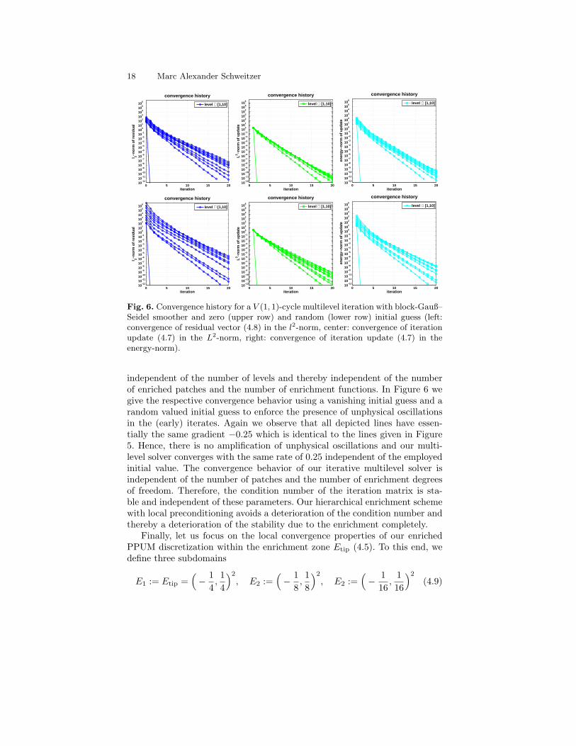
Fig. 6. Convergence history for a V (1, 1)-cycle multilevel iteration with block-Gauß–Seidel smoother and zero (upper row) and random (lower row) initial guess (left:convergence of residual vector (4.8) in the l2-norm, center: convergence of iterationupdate (4.7) in the L2-norm, right: convergence of iteration update (4.7) in theenergy-norm).

independent of the number of levels and thereby independent of the numberof enriched patches and the number of enrichment functions. In Figure 6 wegive the respective convergence behavior using a vanishing initial guess and arandom valued initial guess to enforce the presence of unphysical oscillationsin the (early) iterates. Again we observe that all depicted lines have essen-tially the same gradient −0.25 which is identical to the lines given in Figure5. Hence, there is no amplification of unphysical oscillations and our multi-level solver converges with the same rate of 0.25 independent of the employedinitial value. The convergence behavior of our iterative multilevel solver isindependent of the number of patches and the number of enrichment degreesof freedom. Therefore, the condition number of the iteration matrix is sta-ble and independent of these parameters. Our hierarchical enrichment schemewith local preconditioning avoids a deterioration of the condition number andthereby a deterioration of the stability due to the enrichment completely.

Finally, let us focus on the local convergence properties of our enrichedPPUM discretization within the enrichment zone Etip (4.5). To this end, wedefine three subdomains

E1 := Etip =(− 1

4,14

)2

, E2 :=(− 1

8,18

)2

, E2 :=(− 1

16,

116

)2

(4.9)


Table 2. Relative errors e (4.1) and convergence rates ρ (4.2) with respect to thesubsets E1, E2, and E3 from (4.9).

J dof N eL∞ ρL∞ eL2 ρL2 eH1 ρH1with respect to E1

2 28 4 4.329−2 0.94 3.245−2 1.03 9.040−2 0.723 70 16 3.145−2 0.35 2.061−2 0.50 6.313−2 0.394 178 36 1.058−2 1.17 5.325−3 1.45 2.559−2 0.975 562 100 3.385−3 0.99 1.390−3 1.17 9.671−3 0.856 2002 324 1.018−3 0.95 3.534−4 1.08 3.495−3 0.807 7248 1156 2.965−4 0.96 8.867−5 1.07 1.272−3 0.798 25926 4356 8.477−5 0.98 2.217−5 1.09 4.629−4 0.799 100298 16900 2.387−5 0.94 5.539−6 1.03 1.577−4 0.8010 340007 66564 6.648−6 1.05 1.745−6 0.95 3.933−4 −0.75

with respect to E23 28 4 1.659−2 1.23 1.178−2 1.33 3.599−2 1.004 112 16 4.200−3 0.99 3.707−3 0.83 1.216−2 0.785 252 36 1.209−3 1.54 8.846−4 1.77 4.271−3 1.296 700 100 3.040−4 1.35 2.133−4 1.39 1.472−3 1.047 2268 324 7.329−5 1.21 5.210−5 1.20 5.182−4 0.898 7500 1156 1.819−5 1.17 1.287−5 1.17 1.901−4 0.849 26576 4356 4.555−6 1.09 3.202−6 1.10 7.596−5 0.7210 101194 16900 1.671−6 0.75 1.072−6 0.82 6.574−5 0.11

with respect to E34 28 4 3.567−3 1.69 2.447−3 1.80 1.096−2 1.355 112 16 9.241−4 0.97 7.710−4 0.83 4.124−3 0.706 252 36 2.651−4 1.54 1.803−4 1.79 1.471−3 1.277 700 100 6.244−5 1.42 4.338−5 1.39 5.247−4 1.018 2268 324 1.495−5 1.22 1.056−5 1.20 1.882−4 0.879 7376 1156 3.685−6 1.19 2.612−6 1.18 8.269−5 0.7010 26470 4356 1.794−6 0.56 9.266−7 0.81 6.490−5 0.19

and measure the relative errors (4.1) and convergence rates (4.2) with respectto E1, E2, and E3 of (4.9). According to Section 3.1 we anticipate to finda faster convergence within the enrichment zone tip than for the completedomain Ω. The plots given in Figure 7 and the measured rates displayed inTable 2 clearly show this anticipated behavior. Note that we find about 6digits of relative accuracy in the L2-norm and about 4 digits in the H1-normon E1, i.e. in the vicinity of the singularity. Up to level k = 9 we find ρH1 ≈ 0.8within the subdomains E1, E2, and E3 whereas globally we have the optimalrate ρH1 = 0.5. Hence, we obtain a convergence behavior better than O(h3/2)in the enrichment zone with respect to the energy-norm using enriched linearlocal approximation spaces only.

On level k = 10 however we find a sharp jump in the measured conver-gence rates. For the H1-norm we even find an increase in the error on levelk = 10 compared with level k = 9. Recall from Remark 3 that we may notexpect the measured convergence rates to be constant due to the employedcut-off in the construction of our projection Π∗

i,k which can yield nonnestedlocal approximation spaces. The projection operators Π∗

i,k employed in thiscomputation were based on the identity operator, i.e. on the L2-norm. Hence,we have eliminated enrichment functions whose contribution to the approxi-mation of the L2-norm is insubstantial. This however may not be true for theH1-norm.


102

103

104

105

10−5

10−4

10−3

10−2

convergence history

degrees of freedom

rela

tive

err

or

EH1

L∞

L2

102

103

104

105

10−5

10−4

10−3

10−2

convergence history

degrees of freedom

rela

tive

err

or

EH1

L∞

L2

102

103

104

10−6

10−5

10−4

10−3

10−2

convergence history

degrees of freedom

rela

tive

err

or

EH1

L∞

L2

102

103

104

105

10−5

10−4

10−3

10−2

convergence history

degrees of freedom

rela

tive

err

or

EH1

L∞

L2

102

103

104

105

10−6

10−5

10−4

10−3

10−2

convergence history

degrees of freedom

rela

tive

err

or

EH1

L∞

L2

102

103

104

10−6

10−5

10−4

10−3

10−2

convergence history

degrees of freedom

rela

tive

err

or

EH1

L∞

L2

Fig. 7. Convergence history of the measured relative errors e (4.1) with respect tothe subdomains E1 (left), E2 (center), and E3 (right) given in (4.9) with respect tothe L∞-norm, the L2-norm, the H1-norm, and the energy-norm on the respectivelevel (denoted by E in the legend). The upper row refers to the enriched PPUMusing a preconditioner based on the L2-norm, i.e., the local mass matrix, the lowerrow refers to the enriched PPUM using a preconditioner based on the H1-norm, i.e.,the local stiffness matrix.

According to Remark 2 changing the operator in the construction of Π∗i,k

can impact the cut-off behavior. Constructing the projection Π∗i,k based on

the operator −∆ + I yields an elimination of functions that contribute in-substantially to the H1-norm. This can eliminate (or will at least reduce)the jumps of the measured convergence rates for the H1-norm (and weakernorms). From the numbers given in Table 3 where we employ a projection Π∗

i.k

based on the H1-norm we can clearly observe this anticipated improvement,see also Figure 7. Now we have ρH1 > 0.5 on all levels and ρH1 ≈ 0.7 on levelk = 10 for E1. In Figure 8 we have depicted the enrichment patterns withinEtip for the projections based on the L2-norm and on the H1-norm. For eachpatch ωi,k ⊂ Etip on level k = 9, 10 we have plotted the dimension of the localapproximation space Vi,k, i.e., the number of shape functions ϑm

i,k after cut-off. From these plots we can clearly observe that more enrichment functionsare present in the H1-based approach on level k = 10 than for the L2-basedprojection. On level k = 9 the enrichment patterns are almost identical andso are the measured errors, compare Table 2 and Table 3. On level k = 10however we see a substantial reduction in degrees of freedom due to the cut-


Fig. 8. Enrichment pattern on levels k = 9 (left) and k = 10 (right) within theenrichment zone Etip. Color coded is the dimension of the local approximation spacedim(Vi,k) = card(ϑm

i,k) (denoted as ’resolution’ in the legend). The upper rowrefers to the enriched PPUM using a preconditioner based on the L2-norm, i.e., thelocal mass matrix, the lower row refers to the enriched PPUM using a preconditionerbased on the H1-norm, i.e., the local stiffness matrix. In both cases we used a cut-offparameter of ε = 10−12.

off for the L2-based projection and almost no reduction in degrees of freedomfor the H1-based projection. Hence, the nonnestedness of the respective localapproximation spaces is as expected more severe for the L2-based projectionthan for the H1-based projection.

In summary, the presented hierarchical enrichment scheme yields a globallyoptimal convergence behavior of O(h) in the energy-norm for the uniform h-version of the enriched PPUM without compromising the condition numberof the resulting stiffness matrix. This is achieved by a local preconditionerwhich eliminates the near-null space of an arbitrary local operator. Withinthe enrichment zone the hierarchically enriched PPUM yields a convergencerate of O(h1+δ) in the energy-norm with δ > 0.

5 Concluding Remarks

We presented an automatic hierarchical enrichment scheme for the PPUMwhich yields a stable discretization with optimal convergence properties glob-ally and a kind of superconvergence within the employed enrichment zone.The core ingredients of the presented approach are a geometric hierarchy ofthe cover patches and a special local preconditioner. The construction of thepresented preconditioner relies on the flat-top property of the employed PU.


Table 3. Relative errors e (4.1) and convergence rates ρ (4.2) with respect to thesubsets E1, E2, and E3 from (4.9). The local projections Π∗

i,k are based on theH1-norm.

J dof N eL∞ ρL∞ eL2 ρL2 eH1 ρH1with respect to E1

2 28 4 4.329−2 0.94 3.245−2 1.03 9.040−2 0.723 70 16 3.145−2 0.35 2.061−2 0.50 6.313−2 0.394 178 36 1.058−2 1.17 5.325−3 1.45 2.559−2 0.975 562 100 3.385−3 0.99 1.390−3 1.17 9.671−3 0.856 2002 324 1.018−3 0.95 3.534−4 1.08 3.495−3 0.807 7570 1156 2.974−4 0.93 8.867−5 1.04 1.270−3 0.768 27516 4356 8.477−5 0.97 2.217−5 1.07 4.613−4 0.789 101490 16900 2.387−5 0.97 5.539−6 1.06 1.548−4 0.8410 397538 66564 6.632−6 0.94 1.384−6 1.02 5.701−5 0.73

with respect to E23 28 4 1.659−2 1.23 1.178−2 1.33 3.599−2 1.004 112 16 4.200−3 0.99 3.707−3 0.83 1.216−2 0.785 252 36 1.209−3 1.54 8.846−4 1.77 4.271−3 1.296 700 100 3.040−4 1.35 2.133−4 1.39 1.472−3 1.047 2268 324 7.327−5 1.21 5.209−5 1.20 5.182−4 0.898 8092 1156 1.819−5 1.10 1.287−5 1.10 1.849−4 0.819 27768 4356 4.556−6 1.12 3.200−6 1.13 6.193−5 0.8910 102632 16900 1.142−6 1.06 7.982−7 1.06 2.702−5 0.63

with respect to E34 28 4 3.567−3 1.69 2.447−3 1.80 1.096−2 1.355 112 16 9.241−4 0.97 7.710−4 0.83 4.124−3 0.706 252 36 2.651−4 1.54 1.803−4 1.79 1.471−3 1.277 700 100 6.244−5 1.42 4.337−5 1.39 5.247−4 1.018 2268 324 1.495−5 1.22 1.056−5 1.20 1.882−4 0.879 8092 1156 3.685−6 1.10 2.606−6 1.10 6.133−5 0.8810 27368 4356 9.081−7 1.15 6.484−7 1.14 3.038−5 0.58

Acknowledgement. This work was supported in part by the Sonderforschungsbereich611 Singular phenomena and scaling in mathematical models funded by the DeutscheForschungsgemeinschaft.

References

1. I. Babuska, U. Banerjee, and J. E. Osborn, Survey of Meshless and Gen-eralized Finite Element Methods: A Unified Approach, Acta Numerica, (2003),pp. 1–125.

2. I. Babuska and J. M. Melenk, The Partition of Unity Method, Int. J. Numer.Meth. Engrg., 40 (1997), pp. 727–758.

3. S. Beissel and T. Belytschko, Nodal Integration of the Element-FreeGalerkin Method, Comput. Meth. Appl. Mech. Engrg., 139 (1996), pp. 49–74.

4. T. Belytschko and T. Black, Elastic crack growth in finite elements withminimal remeshing, Int. J. Numer. Meth. Engrg., 45 (1999), pp. 601–620.

5. T. Belytschko, Y. Y. Lu, and L. Gu, Crack propagation by element-freegalerkin methods, Engrg. Frac. Mech., 51 (1995), pp. 295–315.

6. T. Belytschko, N. Moes, S. Usui, and C. Parimi, Arbitrary discontinuitiesin finite elements, Int. J. Numer. Meth. Engrg., 50 (2001), pp. 993–1013.

7. E. Chahine, P. Laborde, J. Pommier, Y. Renard, and M. Salaun, Study ofsome optimal xfem type methods, in Advances in Meshfree Techniques, V. M. A.


Leitao, C. J. S. Alves, and C. A. M. Duarte, eds., vol. 5 of ComputationalMethods in Applied Sciences, Springer, 2007.

8. J. S. Chen, C. T. Wu, S. Yoon, and Y. You, A Stabilized Conforming NodalIntegration for Galerkin Mesh-free Methods, Int. J. Numer. Meth. Engrg., 50(2001), pp. 435–466.

9. J. Dolbow and T. Belytschko, Numerical Integration of the Galerkin WeakForm in Meshfree Methods, Comput. Mech., 23 (1999), pp. 219–230.

10. C. A. Duarte, L. G. Reno, and A. Simone, A higher order generalized fem forthrough-the-thickness branched cracks, Int. J. Numer. Meth. Engrg., 72 (2007),pp. 325–351.

11. C. A. M. Duarte, I. Babuska, and J. T. Oden, Generalized Finite ElementMethods for Three Dimensional Structural Mechanics Problems, Comput. Struc.,77 (2000), pp. 215–232.

12. C. A. M. Duarte, O. N. H. T. J. Liszka, and W. W. Tworzydlo, A gen-eralized finite element method for the simulation of three-dimensional dynamiccrack propagation, Int. J. Numer. Meth. Engrg., 190 (2001), pp. 2227–2262.

13. M. Griebel, P. Oswald, and M. A. Schweitzer, A Particle-Partitionof Unity Method—Part VI: A p-robust Multilevel Preconditioner, in MeshfreeMethods for Partial Differential Equations II, M. Griebel and M. A. Schweitzer,eds., vol. 43 of Lecture Notes in Computational Science and Engineering,Springer, 2005, pp. 71–92.

14. M. Griebel and M. A. Schweitzer, A Particle-Partition of Unity Method—Part II: Efficient Cover Construction and Reliable Integration, SIAM J. Sci.Comput., 23 (2002), pp. 1655–1682.

15. , A Particle-Partition of Unity Method—Part III: A Multilevel Solver,SIAM J. Sci. Comput., 24 (2002), pp. 377–409.

16. , A Particle-Partition of Unity Method—Part V: Boundary Conditions, inGeometric Analysis and Nonlinear Partial Differential Equations, S. Hildebrandtand H. Karcher, eds., Springer, 2002, pp. 517–540.

17. , A Particle-Partition of Unity Method—Part VII: Adaptivity, in Mesh-free Methods for Partial Differential Equations III, M. Griebel and M. A.Schweitzer, eds., vol. 57 of Lecture Notes in Computational Science and En-gineering, Springer, 2006, pp. 121–148.

18. N. Moes, J. Dolbow, and T. Belytschko, A finite element method for crackgrowth without remeshing, Int. J. Numer. Meth. Engrg., 46 (1999), pp. 131–150.

19. J. Nitsche, Uber ein Variationsprinzip zur Losung von Dirichlet-Problemen beiVerwendung von Teilraumen, die keinen Randbedingungen unterworfen sind,Abh. Math. Sem. Univ. Hamburg, 36 (1970–1971), pp. 9–15.

20. J. T. Oden and C. A. Duarte, Clouds, Cracks and FEM’s, Recent Develop-ments in Computational and Applied Mechanics, 1997, pp. 302–321.

21. M. A. Schweitzer, A Parallel Multilevel Partition of Unity Method for EllipticPartial Differential Equations, vol. 29 of Lecture Notes in Computational Scienceand Engineering, Springer, 2003.

22. , An adaptive hp-version of the multilevel particle–partition of unitymethod, Comput. Meth. Appl. Mech. Engrg., (2008). accepted.

Bestellungen nimmt entgegen: Institut für Angewandte Mathematik der Universität Bonn Sonderforschungsbereich 611 Wegelerstr. 6 D - 53115 Bonn Telefon: 0228/73 4882 Telefax: 0228/73 7864 E-mail: [email protected] http://www.sfb611.iam.uni-bonn.de/

Verzeichnis der erschienenen Preprints ab No. 355

355. Löbach, Dominique: On Regularity for Plasticity with Hardening 356. Burstedde, Carsten; Kunoth, Angela: A Wavelet-Based Nested Iteration – Inexact Conjugate Gradient Algorithm for Adaptively Solving Elliptic PDEs 357. Alt, Hans-Wilhelm; Alt, Wolfgang: Phase Boundary Dynamics: Transitions between Ordered and Disordered Lipid Monolayers 358. Müller, Werner: Weyl's Law in the Theory of Automorphic Forms 359. Frehse, Jens; Löbach, Dominique: Hölder Continuity for the Displacements in Isotropic and Kinematic Hardening with von Mises Yield Criterion 360. Kassmann, Moritz: The Classical Harnack Inequality Fails for Non-Local Operators 361. Albeverio, Sergio; Ayupov, Shavkat A.; Kudaybergenov, Karim K.: Description of Derivations on Measurable Operator Algebras of Type I 362. Albeverio, Sergio; Ayupov, Shavkat A.; Zaitov, Adilbek A.; Ruziev, Jalol E.: Algebras of Unbounded Operators over the Ring of Measurable Functions and their Derivations and Automorphisms 363. Albeverio, Sergio; Ayupov, Shavkat A.; Zaitov, Adilbek A.: On Metrizability of the Space of Order-Preserving Functionals 364. Alberti, Giovanni; Choksi, Rustum; Otto, Felix: Uniform Energy Distribution for Minimizers of an Isoperimetric Problem Containing Long-Range Interactions 365. Schweitzer, Marc Alexander: An Adaptive hp-Version of the Multilevel Particle-Partition of Unity Method 366. Frehse, Jens; Meinel, Joanna: An Irregular Complex Valued Solution to a Scalar Linear Parabolic Equation 367. Bonaccorsi, Stefano; Marinelli, Carlo; Ziglio, Giacomo: Stochastic FitzHugh-Nagumo Equations on Networks with Impulsive Noise 368. Griebel, Michael; Metsch, Bram; Schweitzer, Marc Alexander: Coarse Grid Classification: AMG on Parallel Computers

369. Bar, Leah; Berkels, Benjamin; Rumpf, Martin; Sapiro, Guillermo: A Variational Framework for Simultaneous Motion Estimation and Restoration of Motion-Blurred Video; erscheint in: International Conference on Computer Vision 2007 370. Han, Jingfeng; Berkels, Benjamin; Droske, Marc; Hornegger, Joachim; Rumpf, Martin; Schaller, Carlo; Scorzin, Jasmin; Urbach Horst: Mumford–Shah Model for One-to-one Edge Matching; erscheint in: IEEE Transactions on Image Processing 371. Conti, Sergio; Held, Harald; Pach, Martin; Rumpf, Martin; Schultz, Rüdiger: Shape Optimization under Uncertainty – a Stochastic Programming Perspective 372. Liehr, Florian; Preusser, Tobias; Rumpf, Martin; Sauter, Stefan; Schwen, Lars Ole: Composite Finite Elements for 3D Image Based Computing 373. Bonciocat, Anca-Iuliana; Sturm, Karl-Theodor: Mass Transportation and Rough Curvature Bounds for Discrete Spaces 374. Steiner, Jutta: Compactness for the Asymmetric Bloch Wall 375. Bensoussan, Alain; Frehse, Jens: On Diagonal Elliptic and Parabolic Systems with Super-Quadratic Hamiltonians 376. Frehse, Jens; Specovius-Neugebauer, Maria: Morrey Estimates and Hölder Continuity for Solutions to Parabolic Equations with Entropy Inequalities 377. Albeverio, Sergio; Ayupov, Shavkat A.; Omirov, Bakhrom A.; Turdibaev, Rustam M.: Cartan Subalgebras of Leibniz n-Algebras 378. Schweitzer, Marc Alexander: A Particle-Partition of Unity Method – Part VIII: Hierarchical Enrichment

a particle-partition of unity method part viii

Documents