a parallel primal-dual interior-point method for semide …kojima/articles/b-398.pdfa parallel...

Research Reports on Mathematical and Computing SciencesSeries B : Operations Research

Department of Mathematical and Computing SciencesTokyo Institute of Technology

2-12-1 Oh-Okayama, Meguro-ku, Tokyo 152-8552 Japan

A Parallel Primal-Dual Interior-Point Method for Semidefinite ProgramsUsing Positive Definite Matrix Completion

Kazuhide Nakata†, Makoto Yamashita‡, Katsuki Fujisawa? and Masakazu Kojima]

Research Report B-398, November 2003. Revised March 2005 and July 2005

Abstract. A parallel computational method SDPARA-C is presented for SDPs (semidefiniteprograms). It combines two methods SDPARA and SDPA-C proposed by the authors who devel-oped a software package SDPA. SDPARA is a parallel implementation of SDPA and it featuresparallel computation of the elements of the Schur complement equation system and a parallelCholesky factorization of its coefficient matrix. SDPARA can effectively solve SDPs with a largenumber of equality constraints; however, it does not solve SDPs with a large scale matrix vari-able with similar effectiveness. SDPA-C is a primal-dual interior-point method using the positivedefinite matrix completion technique by Fukuda et al, and it performs effectively with SDPs witha large scale matrix variable, but not with a large number of equality constraints. SDPARA-Cbenefits from the strong performance of each of the two methods. Furthermore, SDPARA-C isdesigned to attain a high scalability by considering most of the expensive computations involvedin the primal-dual interior-point method. Numerical experiments with the three parallel softwarepackages SDPARA-C, SDPARA and PDSDP by Benson show that SDPARA-C efficiently solvesSDPs with a large scale matrix variable as well as a large number of equality constraints with asmall amount of memory.

Key words.

Semidefinite Program, Primal-Dual Interior-Point Method, Parallel Computation, Positive DefiniteMatrix Completion, Numerical Experiment, PC Cluster

† Department of Industrial Engineering and Management, Tokyo Institute of Technology,2-12-1 Oh-Okayama, Meguro-ku, Tokyo 152-8552 Japan. [email protected]

‡ Department of Mathematical and Computing Sciences, Tokyo Institute of Technology, 2-12-1 Oh-Okayama, Meguro-ku, Tokyo 152-8552 Japan. [email protected]

? Department of Mathematical Sciences, Tokyo Denki University, Ishizuka, Hatoyama,Saitama 350-0394 Japan. [email protected]

] Department of Mathematical and Computing Sciences, Tokyo Institute of Technology,2-12-1 Oh-Okayama, Meguro-ku, Tokyo 152-8552 Japan. [email protected]

1 Introduction

Semidefinite programs (SDPs) have gained a lot of attention in recent years with applicationsarising from a diverse range of fields including structural optimization, system and control, statis-tics [4], financial engineering [14], and quantum chemistry [24]. The solution of an SDP has beenfound using primal-dual interior-point methods. The development of efficient primal-dual interior-point methods has become a key issue to handle SDPs. For more information on SDP and theprimal-dual interior-point method, see e.g., the papers [21, 29].

Many software packages for solving SDPs with the primal-dual interior-point method havebeen developed and are now available on the Internet. These include SDPA [30] developed bythe authors, and various other packages such as CDSP [6], SeDuMi [25] and SDPT3 [27]. Thesesoftware packages are known to be successful to solve small to medium size SDPs. However,solving large-scale SDPs still remains a difficult problem. Some of the difficult issues involvinglarge-scale SDPs are being unable to store the matrix variables in the computer memory or beingunable to run the algorithm to completion within a practical time scale. A variety of methodshave been proposed to address these issues, including methods in which an iterative solution isapplied to the Schur complement equation system (a linear equation system needed to compute asearch direction vector) [10, 23, 26], interior-point methods that exploit the sparse structure of theproblem [8, 11], a dual interior-point method DSDP [2] and its parallel implementation PDSDP[1], the spectral bundle method [16], first-order nonlinear programming methods [9, 16] and ageneralized augmented Lagrangian method [18].

The amount of data storage needed for the matrix variables of the primal and dual problemscorresponds to the size of the data matrix in the standard form SDP and its dual problem. Whenthe data matrix is sparse, the dual matrix variable inherits this sparsity but in general the matrixvariable of the primal problem forms a completely dense matrix. This is a major drawback of theprimal-dual interior-point method. To address this drawback, SDPA-C (the primal-dual interior-point method using (positive definite) matrix completion) was proposed [12, 22]. This methodwas developed by adapting SDPA to use (positive definite) matrix completion theory to performa sparse factorization of the primal matrix variable, and by incorporating matrix computationsthat take advantage of this sparsity. Since this method does not store the primal matrix variabledirectly, the amount of memory used for the primal matrix variable can be greatly reduced.

The computation times can also be reduced because this method does not perform any com-putation in which the dense matrix is handled directly, so that SDPs having a large but sparsedata matrix can be solved in a shorter time with less memory. But on the other hand, the coeffi-cient matrix of the Schur complement equation system – which is solved at each iteration of theprimal-dual interior-point method – usually forms a dense positive definite matrix even when thedata matrix is sparse (see [3, 28] for some exceptional cases). Furthermore, its size matches thenumber of linear equality constraints in the primal problem. As a result, when SDPA-C is usedfor ordinary large-scale SDP problems, it does not reach a solution efficiently because there arebottlenecks in the computation of the coefficient matrix of the Schur complement equation systemand in the Cholesky factorization.

In the paper [31], we proposed SDPARA (SemiDefinite Programming Algorithm PARAllel Ver-sion). Since the above bottlenecks occur when solving SDPs where the primal problem has a largenumber of linear equality constraints, SDPARA uses tools such as MPI [15] and ScaLAPACK [5]to apply parallel computing to the computation of the coefficient matrix in the Schur complementequation system and to the Cholesky factorization. As a result, the computation times and mem-ory requirements relating to the coefficient matrix of the Schur complement equation system andthe Cholesky factorization have been greatly reduced. However, with this method, since the denseprimal matrix variables are stored and manipulated directly, the increased size of the SDP data

1

matrix results in requiring more time and memory for the computations relating to the primalmatrix variables.

In this paper we propose SDPARA-C, which is obtained by combining and enhancing theprimal-dual interior-point method of SDPA-C using matrix completion theory [12, 22] and theparallel primal-dual interior-point method of SDPARA [31]. This allows us to retain benefits ofSDPA-C and SDPARA while compensating for their drawbacks. The Cholesky factorization of thecoefficient matrix of the Schur complement equation system – which is solved at each iteration ofthe primal-dual interior-point method – is made to run in parallel in the same way as in [31]. Also,the computation of this coefficient matrix is improved so that the load is kept equally balancedbased on the method proposed in [31]. Furthermore, we arrive at a highly scalable implementationby employing parallel processing for all the computations that take up most of the computationtime in other places where bottlenecks are liable to occur. This makes it possible to solve SDPswith large sparse data matrices and large numbers of linear equality constraints in less time andwith less memory.

This paper is organized as follows. In section 2, we present an overview of SDPA-C andSDPARA and their drawbacks. In section 3 we propose SDPARA-C. In section 4 we performnumerical experiments to evaluate the efficiency of SDPARA-C, and in section 5 we present ourconclusions.

2 Previous studies

In this section we first discuss the standard interior-point method for solving SDPs. We thenpresent an overview of techniques in which parallel processing is applied to the primal-dual interior-point method involving the use of matrix completion theory as proposed in the papers [12, 22],and the primal-dual interior-point method proposed in the paper [31], and we describe some issuesassociated with these techniques.

2.1 Solving SDPs with the primal-dual interior-point method

Let Sn denote the vector space of n × n symmetric matrices. For a pair of matrices X,Y ∈ S n,the inner product is defined as X •Y =

∑ni=1

∑nj=1 XijYij. We use the notation X ∈ Sn

+ (Sn++) to

indicate that X ∈ Sn is positive semidefinite (or positive definite). Given Ap ∈ Sn (p = 0, 1, . . . ,m)and b = (b1, b2, . . . , bm)T ∈ R

m, the standard form SDP is written as follows:

minimize A0 • X

subject to Ap • X = bp (p = 1, 2, . . . ,m), X ∈ Sn+

}. (1)

The corresponding dual problem is as follows:

maximize

m∑

p=1

bpzp

subject to

m∑

p=1

Apzp + Y = A0, Y ∈ Sn+

. (2)

It is known that primal-dual interior-point methods are capable of solving these problemsin polynomial time. There have been proposed many primal-dual interior-point methods suchas the path-following method and the Mehrotra-type predictor-corrector method, and varioustypes of search directions used therein such as the HRVW/KSH/M search direction and the NTsearch direction. Although most of implementation of primal-dual interior-point methods employ

2

the Mehrotra-type predictor-corrector method due to its computational efficiency, we choose asimpler path-following method to effectively exploit sparsity of SDPs using the matrix completiontechnique; the Mehrotra-type predictor-corrector method, which is more sophisticated than thepath-following method, would not fit the matrix completion technique [12, 22]. We also use theHRVW/KSH/M search direction. The HRVW/KSH/M search direction (dX , dY , dz) ∈ S n ×Sn ×R

m is defined as “the Newton-type direction toward the central path”, and is computed by reducingit to a system of linear equations in the vector variable dz ∈ R

m known as the Schur complementequation system [11, 19]. The path-following primal-dual interior-point method with the use ofthe HRVW/KSH/M search direction can be summarized as described below.

Algorithm 2.1: The basic primal-dual interior-point method

Step 0: Set up parameters γ1, γ2 ∈ (0, 1), choose a starting point (X,Y , z) ∈ Sn++×Sn

++×Rm,

and set µ := 1nX • Y .

Step 1: Compute the search direction (dX, dY , dz) ∈ Sn × Sn × Rm.

Step 1a: Set µ := γ1µ and compute the residuals r ∈ Rm, R ∈ Sn, C ∈ R

n×n defined asfollows:

rp := bp − Ap • X (p = 1, 2, . . . ,m),R := A0 −

∑mp=1 Apzp − Y , C := µI − XY .

Step 1b: Compute the m × m matrix B and the vector s ∈ Rm.

Bpq := Ap • XAqY−1 (p, q = 1, 2, . . . ,m), (3)

sp := rp − Ap • (C − XR)Y −1 (p = 1, 2, . . . ,m).

It is known that B is usually a fully dense positive definite symmetric matrix [11] (see[3, 28] for some exceptional cases).

Step 1c: Solve the Schur complement equation system Bdz = s to find dz.

Step 1d: Compute dY and dX from dz.

dY := R −m∑

p=1

Apdzp, dX := (C − XdY )Y −1, dX := (dX + dXT)/2.

Step 2: Determine the largest step size αp, αd in the search direction (dX , dY , dz).

αp := −1.0/λmin(√

X−1

dX√

X−T

), αd := −1.0/λmin(√

Y−1

dY√

Y−T

).

where√

G denotes a matrix that satisfies√

G√

GT

= G ∈ Sn++, and λmin(H) is the mini-

mum eigenvalue of matrix H ∈ Sn.

Step 3: Update the iteration point (X,Y , z) from the search direction and the step size, andreturn to Step 1.

X := X + γ2αpdX ∈ Sn++, Y := Y + γ2αddY ∈ Sn

++, z := z + γ2αddz.

A characteristic of Algorithm 2.1 is that the matrices X and Y obtained at each iteration arepositive definite, which is how the interior-point method gets its name. In practice, the efficiencyof Algorithm 2.1 will greatly differ depending on what sort of algorithms and data structures areused. Our aim is to solve large-scale sparse SDPs with the smallest possible computation time andmemory usage. To clarify the following discussion, we classify the parts that consume the bulk ofthe computation time into four types based on SDPA6.0 [30]

3

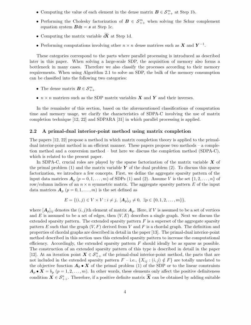
• Computing the value of each element in the dense matrix B ∈ Sm++ at Step 1b.

• Performing the Cholesky factorization of B ∈ Sm++ when solving the Schur complement

equation system Bdz = s at Step 1c.

• Computing the matrix variable dX at Step 1d.

• Performing computations involving other n × n dense matrices such as X and Y−1.

These categories correspond to the parts where parallel processing is introduced as describedlater in this paper. When solving a large-scale SDP, the acquisition of memory also forms abottleneck in many cases. Therefore we also classify the processes according to their memoryrequirements. When using Algorithm 2.1 to solve an SDP, the bulk of the memory consumptioncan be classified into the following two categories:

• The dense matrix B ∈ Sm++

• n × n matrices such as the SDP matrix variables X and Y and their inverses.

In the remainder of this section, based on the aforementioned classifications of computationtime and memory usage, we clarify the characteristics of SDPA-C involving the use of matrixcompletion technique [12, 22] and SDPARA [31] in which parallel processing is applied.

2.2 A primal-dual interior-point method using matrix completion

The papers [12, 22] propose a method in which matrix completion theory is applied to the primal-dual interior-point method in an efficient manner. These papers propose two methods – a comple-tion method and a conversion method – but here we discuss the completion method (SDPA-C),which is related to the present paper.

In SDPA-C, crucial roles are played by the sparse factorization of the matrix variable X ofthe primal problem (1) and the matrix variable Y of the dual problem (2). To discuss this sparsefactorization, we introduce a few concepts. First, we define the aggregate sparsity pattern of theinput data matrices Ap (p = 0, 1, . . . ,m) of SDPs (1) and (2). Assume V is the set {1, 2, . . . , n} ofrow/column indices of an n× n symmetric matrix. The aggregate sparsity pattern E of the inputdata matrices Ap (p = 0, 1, . . . ,m) is the set defined as

E = {(i, j) ∈ V × V : i 6= j, [Ap]ij 6= 0, ∃p ∈ {0, 1, 2, . . . ,m}},

where [Ap]ij denotes the (i, j)th element of matrix Ap. Here, if V is assumed to be a set of verticesand E is assumed to be a set of edges, then (V,E) describes a single graph. Next we discuss theextended sparsity pattern. The extended sparsity pattern F is a superset of the aggregate sparsitypattern E such that the graph (V, F ) derived from V and F is a chordal graph. The definition andproperties of chordal graphs are described in detail in the paper [13]. The primal-dual interior-pointmethod described in this section uses this extended sparsity pattern to increase the computationalefficiency. Accordingly, the extended sparsity pattern F should ideally be as sparse as possible.The construction of an extended sparsity pattern of this type is described in detail in the paper[12]. At an iteration point X ∈ Sn

++ of the primal-dual interior-point method, the parts that arenot included in the extended sparsity pattern F – i.e., {Xij : (i, j) /∈ F} are totally unrelated tothe objective function A0 • X of the primal problem (1) of the SDP or to the linear constraintsAp • X = bp (p = 1, 2, . . . ,m). In other words, these elements only affect the positive definiteness

condition X ∈ Sn++. Therefore, if a positive definite matrix X can be obtained by adding suitable

4

values to the parts {Xij : (i, j) /∈ F} that are not included in the extended sparsity pattern F , then

this matrix X can be used as the iteration point. This process of arriving at a positive definitematrix by determining suitable values is called (positive definite) matrix completion. According to

matrix completion theory, when (V, F ) is a chordal graph, the matrix X that has been subjected topositive definite matrix completion in the way to maximize its determinant value can be factorizedas X = M

−TM

−1 [12]. Here M is a sparse matrix that only has nonzero elements in parts ofthe extended sparsity pattern F , and forms a matrix in which a suitable permutation is made tothe rows and columns of a lower triangular matrix. Furthermore, the matrix variable Y can befactorized as Y = NN

T . Here N is a sparse matrix that only has nonzero elements in parts ofthe extended sparsity pattern F , and forms a matrix in which a suitable permutation is made tothe rows and columns of a lower triangular matrix. In the primal-dual interior-point method thatuses matrix completion theory as proposed in the paper [22], the computations at each step ofAlgorithm 2.1 are performed using this sparse factorization as much as possible. In particular,the sparse matrices M and N are stored instead of the conventional dense matrices X and Y

−1,and this sparsity is exploited when implementing the primal-dual interior-point method. Note alsothat both M

−1 and N−1 become dense in general.

For this paper we fully updated SDPA-C software package which incorporates new matrixcompletion techniques based on SDPA 6.0 [30], which is the latest version of SDPA. Table 1 showsnumerical results obtained when solving two SDPs with SDPA 6.0 and with SDPA-C. Problem Aand B are SDP relaxations of maximum cut problems and maximum clique problems, respectivelywhich are described in section 4. The size of problem A is n = 1000,m = 1000, and the size ofproblem B is n = 1000,m = 1891.

Table 1: The relative practical benefits of SDPA and SDPA-C

Problem A Problem BSDPA SDPA-C SDPA SDPA-C

Computation of B 2.2s 20.3s 82.0s 662.8sCholesky factorization of B 3.5s 3.7s 25.3s 34.1s

Computation of dX 51.7s 9.2s 69.4s 32.6sDense matrix computation 96.1s 1.1s 125.7s 2.6s

Total computation time 157s 34s 308s 733s

Storage of B 8MB 8MB 27MB 27MBStorage of n × n matrix 237MB 4MB 237MB 8MB

Total memory usage 258MB 14MB 279MB 39MB

To solve problem A, the SDPA software needed 15 iterations of the primal-dual interior-pointmethod and the SDPA-C software needed 16. For problem B, SDPA needed 20 iterations andSDPA-C needed 27. The reason why SDPA-C needed more iterations is that SDPA is a Mehrotra-type predictor-corrector primal-dual interior-point method, whereas SDPA-C is a simpler path-following primal-dual interior-point method. In SDPA-C the dense matrices X and Y

−1 are notstored directly, but instead the sparse factorizations M

−TM

−1 and N−T

N−1 are used. Conse-

quently, less time is needed for the computation of dX and the computations involving dense n×nmatrices. Furthermore, there is no need to store any n×n dense matrices, so the memory require-ments are correspondingly much lower than those of SDPA. However, more computation time isneeded to evaluate each element of the coefficient matrix B ∈ Sm

++ of the Schur complement equa-tion system Bdz = s. This is because the matrices X and Y

−1 are not stored directly, making it

5

impossible for SDPA-C to use computational methods that exploit the sparsity of the input datamatrices Ap (p = 1, 2, . . . ,m) used in SDPA [11]. Similar computations are used for the Choleskyfactorization of B, so compared with conventional SDPA the computation time per iteration andthe memory requirements are unchanged. Consequently there are some cases (e.g., problem A)where SDPA-C achieves substantial reductions in computation times and memory requirementscompared with SDPA, while there are other cases (e.g., problem B) where although the memoryrequirements are substantially lower, the overall computation time is larger. In general to solve asparse SDP with large n, SDPA-C needs much less memory than SDPA. On the other hand, thecomputation time of SDPA-C also includes the increased amount of computation needed to obtainthe value of each element of B ∈ Sm

++, so the benefits of matrix completion can sometimes bemarginal or even non-existent depending on the structure of the problem. In SDPs with a largem, most of the overall computation times and memory requirements are taken up by the Choleskyfactorization of B ∈ Sm

++, so in such cases the use of matrix completion has little effect.

2.3 The parallel computation of primal-dual interior-point methods

The paper [31] proposes the SDPARA software which is based on SDPA and which solves SDPsby executing the primal-dual interior-point method on parallel CPUs (PC clusters). In SDPARA,two parts – the computation of the value of each element of the coefficient matrix B ∈ Sm

++ ofthe Schur complement equation system Bdz = s at step 1b of Algorithm 2.1 and the Choleskyfactorization of B ∈ Sm

++ at step 1c – are performed by parallel processing.We first describe how parallel processing can be used to obtain the values of each element

in B ∈ Sm++. Each element of B is defined by equation (3), where each row can be computed

independently. Consequently, it can be processed in parallel by allocating each row to a differentCPU. To represent the distribution of processing to a total of u CPUs, the m indices {1, 2, · · · ,m}are partitioned into Pi (i = 1, 2, · · · , u) groups. That is,

∪ui=1Pi = {1, 2, · · · ,m}, Pi ∩ Pj = ∅ if i 6= j.

Here, the ith CPU computes each element in the pth row of B (p ∈ Pi). The ith CPU only needsenough memory to store the pth row of B (p ∈ Pi). The allocation of rows Pi (i = 1, 2, . . . , u) tobe processed by each CPU should be done so as to balance the loads as evenly as possible andreduce the amount of data transferred. In SDPARA the allocation is performed sequentially fromthe top down, mainly for practical reasons. In other words,

Pi = {x ∈ {1, 2, · · · ,m} | x ≡ i (mod u)} (i = 1, 2, . . . , u). (4)

In general, since m (the size of B) is much larger than u (the number of CPUs), reasonably goodload balancing can still be achieved with this simple method [31].

Next, we discuss how the Cholesky factorization of the coefficient matrix B of the Schur com-plement equation system Bdz = s can be performed in parallel. In SDPARA, this is done bycalling the parallel Cholesky factorization routine in the ScaLAPACK parallel numerical computa-tion library [5]. In the Cholesky factorization of the matrix, the load distribution and the quantityof data transferred are greatly affected by the way in which the matrix is partitioned. In ScaLA-PACK’s parallel Cholesky factorization, the coefficient matrix B is partitioned by block-cyclicpartitioning and each block is allocated to and stored in each CPU.

We now present the results of numerical experiments in which the ordinary characteristicsof SDPARA are well expressed. Table 2 shows the numerical results obtained when two typesof SDPs were solved with SDPA6.0 and SDPARA. With SDPARA the parallel processing wasperformed using 64 CPUs – the computation times and memory requirements are shown for one

6

of these CPUs. In SDPARA, the time taken up by transmitting data in block-cyclic partitionedformat for the parallel Cholesky factorization of B ∈ Sm

++ performed one row at a time on eachCPU is included in the term “Computation of B”. Problem C is an SDP relaxation of maximumclique problems which is described in section 4. The size of problem C is n = 300,m = 4375, whileproblem B is the same as the problem used in the numerical experiment of Table 1, with n = 1000and m = 1891.

Table 2: Numerical comparison between SDPA and SDPARA

Problem C Problem BSDPA SDPARA SDPA SDPARA






As Table 2 shows, the time taken for the computation of B and the Cholesky factorization ofB is greatly reduced. (The number of iterations in the primal-dial interior-point method is thesame for each problem in SDPA and SDPARA.) Also, since B ∈ Sm

++ is stored by partitioning itbetween the CPUs, the amount of memory needed to store B at each CPU is greatly reduced. Onthe other hand, there is no change in the computation times associated with the n×n dense matrixcomputation such as the computation of dX. Also, the amount of memory needed to store then× n matrix on each CPU is the same as in SDPA. In SDPARA, MPI is used for communicationbetween the CPUs. Since additional time and memory are consumed when MPI is started up, itcauses the overall computation times and memory requirements to increase slightly. In an SDPwhere m is large and n is small, as in problem C, it becomes possible to process the parts relating tothe Schur complement equation system Bdz = s – which would otherwise require a large amountof time and memory – very efficiently by employing parallel processing, and great reductions canalso be made to the overall computation times and memory requirements. On the other hand, in aproblem where n is large, as in problem B, large amounts of time and memory are consumed in theparts where the n×n dense matrix is handled. Since these parts are not performed in parallel, it isnot possible to greatly reduce the overall computation times or memory requirements. Generallyspeaking, SDPARA can efficiently solve SDPs with large m where time is taken up by the Choleskyfactorization of B ∈ Sm

++ and dense SDPs where a large amount of time is needed to compute eachelement of B. But in an SDP with large n, the large amounts of computation time and memorytaken up in handling the n × n dense matrix make it difficult for SDPARA to reach a solution inthe same way as SDPA.

3 The parallel computation of primal-dual interior-point methods

using matrix completion

In this section we propose the SDPARA-C software package, which is based on SDPA-C as de-scribed in section 2.2 and which solves SDP problems by executing the primal-dual interior-point

7

method on parallel CPUs (PC clusters). The parallel computation of B ∈ Sm++ is discussed in

section 3.1, and the parallel computation of dX is discussed in section 3.2. After that, section 3.3summarizes the characteristics of SDPARA-C.

3.1 Computation of the coefficient matrix

In the paper [22], three methods are proposed for computing the coefficient matrix B ∈ Sm++ of the

Schur complement equation system Bdz = s. We chose to develop our improved parallel methodbased on the method discussed in section 5.2 of the paper [22]. Each element of B ∈ Sm

++ ands ∈ R

m computed in the following way:

Bpq :=

n∑

k=1

(M−TM

−1ek)

TAq(N

−TN

−1Uk[Ap])

+

n∑

k=1

(N−TN

−1ek)

TAq(M

−TM

−1Uk[Ap]) (p, q = 1, 2, . . . ,m),

sp := bp +n∑

k=1

(M−TM

−1ek)

TR(N−T

N−1Uk[Ap])

+

n∑

k=1

(N−TN

−1ek)

TR(M−T

M−1Uk[Ap])

−n∑

k=1

2µeTk N

−TN

−1Uk[Ap] (p = 1, 2, . . . ,m).

(5)

The diagonal part of matrix Ap is denoted by T , and the upper triangular part excluding thediagonal is denoted by U . In equation (5), Uk[Ap] represents the kth column of the upper triangularmatrix 1

2T + U , and ek ∈ Rn denotes a vector in which the kth element is 1 and all the other

elements are 0. This algorithm differs from the method proposed in section 5.2 of the paper [22] intwo respects. One is that the computations are performed using only the upper triangular matrixpart of matrix Ap. When Uk[Ap] is a zero vector, there is no need to perform computationsinvolving its index k. Comparing the conventional method and the method of equation (5), it isimpossible to generalize which has fewer indices k to be computed. The other difference is thatwhereas X is subjected to a clique sparse factorization M

−TDM

−1 in section 5.2 of the paper[22], we implemented the sparse factorization M

−TM

−1. Because the computation costs arealmost same and the sparse factorization M

−TM

−1 is implemented more easily than the cliquesparse factorization M

−TDM

−1.Here, equation (5) can be used to compute B ∈ Sm

++ independently for each row in the sameway as in the discussion of SDPARA in section 2.3. Therefore, in SDPARA-C it is possible toallocate the computation of B ∈ Sm

++ to each CPU one row at a time. This allocation is performedin the same way as in equation (4) of section 2.3. However, when using equation (5) to perform thecomputations, the number of nonzero column vectors in Uk[Ap] strongly affects the computationalefficiency. Normally, since the number of nonzero vectors in Uk[Ap] is not fixed, it is possible thatlarge variations may occur in the computation time on each CPU when the allocation to eachCPU is performed as described above. For example, when there is just one identity matrix in theconstraint matrices, this matrix may be regarded as a sparse matrix but equation (5) still has tobe computed for every value of index k from 1 to n. To avoid such circumstances, it is betterto process rows that are likely to involve lengthy computation and disrupt the load balance inparallel not by a single CPU but by multiple CPUs. The set of indices of such rows is defined asQ ⊂ {1, 2, . . . ,m}. The allocation Kp

i is set for every p ∈ Q and every i = 1, 2, · · · , u as follows:

∪ui=1K

pi = {k ∈ {1, 2, . . . , n} | Uk[Ap] 6= 0}, Kp

i ∩ Kpj = ∅ if i 6= j

8

At the ith CPU, the following computation is only performed for indices k contained in K pi in

equation (5), with the results stored in a working vector w ∈ Rm and a scalar g ∈ R.

wq :=∑

k∈Kp

i

(M−TM

−1ek)

TAq(N

−TN

−1Uk[Ap])

+∑

k∈Kp

i

(N−TN

−1ek)

TAq(M

−TM

−1Uk[Ap]) (q = 1, 2, . . . ,m),

g :=∑

k∈Kp

i

(M−TM

−1ek)

TR(N−T

N−1Uk[Ap])

+∑

k∈Kp

i

(N−TN

−1ek)

TR(M−T

M−1Uk[Ap])

−∑

k∈Kp

i

2µeTk N

−TN

−1Uk[Ap].

After that, the values of w and g computed at each CPU are sent to the jth CPU that wasoriginally scheduled to process the vector of the pth row of B ∈ Sm

++ (p ∈ Pj), where they areadded together. Therefore, the pth row of B ∈ Sm

++ is stored at the jth CPU (p ∈ Pj). Thus,the algorithm for computing the coefficient matrix B ∈ Sm

++ of the Schur complement equationsystem and the right hand side vector s ∈ R

m at the ith CPU is as follows:

Computation of B and s at the ith CPU

Set B := O, s := b

for p ∈ QSet w = 0 and g = 0for k ∈ Kp

i

Compute v1 := M−T

M−1

ek and v2 := N−T

N−1Uk[Ap]

Compute v3 := N−T

N−1

ek and v4 := M−T

M−1Uk[Ap]

for q = 1, 2, . . . ,mCompute vT

1 Aqv2 + vT3 Aqv4 and add to wq

end(for)Compute vT

1 Rv2 + vT3 Rv4 − 2µeT

k v2 and add to gend(for)Send w and g to the jth CPU (p ∈ Pj) and add them together

end(for)for p ∈ Pi − Q

for k = 1, 2, . . . , n where Uk[Ap] 6= 0

Compute v1 := M−T

M−1

ek and v2 := N−T

N−1Uk[Ap]

Compute v3 := N−T

N−1

ek and v4 := M−T

M−1Uk[Ap]

for q = 1, 2, . . . ,mCompute vT

1 Aqv2 + vT3 Aqv4 and add to Bpq

end(for)Compute vT

1 Rv2 + vT3 Rv4 − 2µeT

k v2 and add to sp

end(for)end(for)

As a result of this computation, the Schur complement equation system B ∈ Sm++ is partitioned

and stored row by row on each CPU. After that, B ∈ Sm++ is sent to each CPU in block-cyclic

partitioned form, and the Cholesky factorization is then performed in parallel.

9

3.2 Computation of the search direction

Here we discuss the parallel computation of the matrix variable dX at step 1d of Algorithm 2.1.In the paper [22] it was proposed that dX should be computed in separate columns as follows:

[dX ]∗k := µN−T

N−1

ek − [X ]∗k − M−T

M−1dY N

−TN

−1ek. (6)

Here [A]∗k denotes the kth column of A. It has been shown that if a nonlinear search is performedhere instead of the linear search performed at step 3 of Algorithm 2.1, then it is only necessary tostore the values of the extended sparsity pattern parts of dX. Since [dX ]∗k and [dX ]∗k′ (k 6= k′)can be computed independently using the formula (6), it should be possible to split the matrixinto columns and process these columns in parallel on multiple CPUs. The computational loadassociated with computing a single column is more or less constant. Therefore, by uniformlydistributing columns to multiple CPUs, the computation can be performed in parallel with auniformly balanced load.

The computation of columns of dX at the ith CPU is performed as shown below. Here, theCPU allocations Ki (i = 1, 2, · · · , u) are determined as follows:

Ki = {x ∈ {1, 2, · · · , n} | (i − 1)[

nu

]< x ≤ i[n

u]} (i = 1, 2, . . . , u − 1),

Ku = {x ∈ {1, 2, · · · , n} | (u − 1)[

nu

]< x}.

and the ith CPU computes the pth column of dX (p ∈ Ki).

Computation of dX at the ith CPU

Set dX := −X

for k ∈ Ki

Compute v := µN−T

N−1

ek − M−T

M−1dZN

−TN

−1ek

Add v to dX∗k

end(for)Transmit the column vector computed at each CPU to all the other CPUs

At the end of this algorithm, the column vector computed at each CPU is sent to all the otherCPUs. At this time, since only the extended sparsity pattern parts of dX are needed, these arethe only parts that have to be sent to the other CPUs. Therefore, this part of the data transfercan be performed at high speed.

3.3 Characteristics

Table 3 shows the computation time of each part and the memory requirements when problemB used in the numerical experiments of Tables 1 and 2 (n = 1000,m = 1891) is solved withSDPARA-C. In this experiment, the parallel processing was performed using 64 CPUs. To facilitatecomparison, the results obtained with SDPA 6.0, SDPA-C and SDPARA as shown in Tables 1 and2 are also reproduced here. In the results obtained with SDPARA and SDPARA-C, the time takenup by transmitting data in block-cyclic partitioned format for the parallel Cholesky factorizationof the coefficient matrix B ∈ Sm

++ of the Schur complement equation system performed one rowat a time on each CPU is included in the term “Computation of B”. Also, the time taken to sendthe results of computing dX obtained at each CPU to all the other CPUs is included in the term“Computation of dX”.

10

Table 3: Numerical comparison between SDPA, SDPA-C, SDPARA and SDPARA-C

Problem BSDPA SDPA-C SDPARA SDPARA-C






The number of iterations of the primal-dual interior-point method was 20 when the problem wassolved by SDPA and SDPARA, and 27 when solved by SDPA-C and SDPARA-C. The reason whymore iterations were required by the primal-dual interior-point methods using matrix completion isthat these are simple path-following primal-dual interior-point methods. Section 2.1 mentions thefour parts that take up most of the computation time and the two parts that take up most of thememory requirements when an SDP is solved by a primal-dual interior point method. In Table 3,we are able to confirm that the problem is processed efficiently in all these parts by SDPARA-C. SDPARA-C uses MPI for communication between CPUs in the same way as SDPARA. Sinceadditional time and memory are consumed when MPI is started up and executed, it causes theoverall computation times and memory requirements to increase. This is why the overall amount ofmemory used by SDPARA-C is greater than that of SDPA-C. As Table 3 shows, the computationtimes involved in the “Computation of B” of SDPARA-C does not necessarily improve when itis compared to that of SDPARA. The next section shows the results of numerical experiments inwhich a variety of problems were solved by SDPARA-C.

4 Numerical experiments

This section presents the results of numerical experiments. In section 4.1, 4.2 and 4.3, the numericalexperiments performed on the Presto III PC cluster at the Matsuoka Laboratory in the TokyoInstitute of Technology. Each node of this cluster consists of an Athlon 1900+ (1.6 GHz) CPUwith 768 MB of memory. The nodes are connected together by a Myrinet 2000 network, which isfaster and performs better than Gigabit Ethernet. In section 4.4 and 4.5, the numerical experimentsperformed on the SDPA PC cluster at the Fujisawa Laboratory in the Tokyo Denki University.Each node of this cluster consists of a Dual Athlon MP 2400+ (2GHz) CPU with 1GB of memory.The nodes are connected together by 1000BASE-T.

In these experiments we evaluated three types of software. One was the SDPARA-C softwareproposed in this paper. The second was SDPARA [31]. The third was PDSDP ver.4.6, as usedin the numerical experiments of the paper [1], which employs the dual interior-point method onparallel CPUs. SDPARA-C and SDPARA used ScaLAPACK ver.1.7 and ATLAS ver.3.4.1. Andthe block size used with ScaLAPACK is 40 and other options are default settings. In all theexperiments apart from those described in section 4.5, the starting point of the interior-pointmethod was chosen to be X = Y = 100I , z = 0. As the termination conditions, the algorithmswere run until the relative dual gap in SDPARA-C and SDPARA was 10−7 or less.

11

The SDPs used in the experiments were:

• SDP relaxations of randomly generated maximum cut problems.

• SDP relaxations of randomly generated maximum clique problems.

• Randomly generated norm minimization problems.

• Some benchmark problems from SDPLIB [7].

• Some benchmark problems from the 7th DIMACS implementation challenge.

The SDP relaxations of maximum cut problems and norm minimization problems were the sameas the problems used in the experiments of the paper [22].

SDP relaxations of maximum cut problems: Assume G = (V,E) is an undirected graph,where V = {1, 2, . . . , n} is a set of vertices and E ⊂ {(i, j) : i, j ∈ V, i < j} is a set of edges. Also,assume that weights Cij = Cji ((i, j) ∈ E) are also given. An SDP relaxation of a maximum cutproblem is then given by

minimize −A0 • X

subject to Eii • X = 1/4 (i = 1, 2, . . . , n),X ∈ Sn

+,(7)

where Eii is an n×n matrix where the element at (i, i) is 1 and all the other elements are 0. Also,we define A0 = diag(Ce) − C.

SDP relaxations of maximum clique problems: Assume G = (V,E) is an undirected graphas in the maximum cut problem. An SDP relaxation of the maximum clique SDP problem is thengiven by

minimize −E • X

subject to Eij • X = 0 ((i, j) /∈ E),I • X = 1, X ∈ Sn

+,(8)

where E is an n × n matrix where all the elements are 1, and E ij is an n × n matrix where the(i, j)th and (j, i)th elements are 1 and all the other elements are 0. Since the aggregate sparsitypattern and extended sparsity pattern are dense patterns in this formulation, the problem is solvedafter performing the transformation proposed in section 6 of the paper [12].

Norm minimization problem: Assume F i ∈ Rq×r (i = 1, 2, . . . , p). The norm minimization

problem is then defined as follows:

minimize

∥∥∥∥∥F 0 +

p∑

i=1

F iyi

∥∥∥∥∥ subject to yi ∈ R (i = 1, 2, . . . , p).

where ‖G‖ is the spectral norm of G; i.e., the square root of the maximum eigenvector of GTG.

This problem can be transformed into the following SDP:

maximize −zp+1

subject to

p∑

i=1

(O F

Ti

F i O

)zi +

(I O

O I

)zp+1 +

(O F

T0

F 0 O

)= Y ,

Y ∈ Sq+r+ .

(9)

12

In section 4.1 we verify the scalability of parallel computations in SDPARA-C, SDPARA andPDSDP. In section 4.2 we investigate how the sparsity of the extended sparsity pattern of an SDPaffects the efficiency of the three software packages. In section 4.3 we investigate how large SDPscan be solved. And finally in sections 4.4 and 4.5 we select a number of SDPs from the SDPLIB[7] problems and DIMACS challenge problems and solve them using SDPARA-C.

4.1 Scalability

In this section we discuss the results of measuring the computation times required to solve anumber of SDPs with clusters of 1, 2, 4, 8, 16, 32 and 64 PCs. The problems that were solvedare listed in Table 4. In this table, n and m respectively represent the size of matrix variables X

and Y and the number of linear constraints in the primal problem (1). The numerical results areshown in Figures 1, 2, 3 and Table 5.

Table 4: Problems solved in the experiments.Problem n m

Cut(10 ∗ 100) 1000 1000 10 × 100 lattice graph maximum cut (7)Cut(10 ∗ 500) 5000 5000 10 × 500 lattice graph maximum cut (7)Clique(10 ∗ 100) 1000 1891 10 × 100 lattice graph maximum clique (8)Clique(10 ∗ 200) 2000 3791 10 × 200 lattice graph maximum clique (8)Norm(10 ∗ 990) 1000 11 Norm minimization of ten 10 × 990 matrices (9)Norm(5 ∗ 995) 1000 11 Norm minimization of ten 5 × 995 matrices (9)qpG11 1600 800 SDPLIB[7] problemmaxG51 1000 1000 SDPLIB[7] problemcontrol10 150 1326 SDPLIB[7] problemtheta6 300 4375 SDPLIB[7] problem

In Figure 1, the horizontal axis shows the number of CPUs and the vertical axis shows thelogarithmic computation time. From the numerical results it can be confirmed that parallel com-putation performed with SDPARA-C has a very high level of scalability. Although the scalabilitybecomes worse as the number of CPUs increases and the computation time is in the region of afew tens of seconds, this is due to factors such as disruption of the load balance of each CPU andan increase in the proportion of time taken up by data transfers.

Next, we performed similar numerical experiments with SDPARA. The results of these exper-iments are shown in Figure 2. In SDPARA, the “Cut(10 ∗ 500)” and “Clique(10 ∗ 200)” problemscould not be solved because there was insufficient memory. As mentioned in section 2.3, in SD-PARA the computation of the coefficient matrix B ∈ Sm

++ of the Schur complement equationsystem of size m and the Cholesky factorization thereof are performed in parallel. Therefore, theeffect of parallel processing is very large for the “control10” and “theta6” problems where m islarge compared to n. On the other hand, in the other problems where m is at most only twiceas large as n, parallel processing had almost no effect whatsoever. Compared with the numericalresults of SDPARA-C shown in Figure 1, SDPARA produced solutions faster than SDPARA-C forthe two SDPs with small n (“control10” and “theta6”). In the “Clique(10 ∗ 100)” problem, thecomputation time of SDPARA was smaller with fewer CPUs, but with a large number of CPUsthe computation time was lower in SDPARA-C. This is because parallel processing is applied tomore parts in SDPARA-C, so it is more able to reap the benefits of parallel processing. For theother problems, SDPARA-C performed better.

Next, we performed similar numerical experiments with PDSDP [1]. The results of these

13

1

10

100

1000

10000

100000

1 2 4 8 16 32 64

Com

puta

tion

time

(sec

onds

)

No. of CPUs

Cut(10*100)Cut(10*500)

Clique(10*100)Clique(10*200)Norm(10*990)Norm(5*995)

qpG11maxG51

control10theta6

Figure 1: Scalability of SDPARA-C applied to problems listed in Table 4

1

10

100

1000

10000

100000

1 2 4 8 16 32 64

Com

puta

tion

time

(sec

onds

)

No. of CPUs

Cut(10*100)Cut(10*500)


qpG11maxG51

control10theta6

Figure 2: Scalability of SDPARA applied to problems listed in Table 4

experiments are shown in Figure 3. PDSDP is a software package that employs the dual interior-point method on parallel CPUs. However, according to the numerical results shown in Figure 3,it appears that this algorithm is not particularly scalable for some problems. Its performanceis similar to that of SDPARA for SDPs such as “control10” and “theta6” where m is large and

14

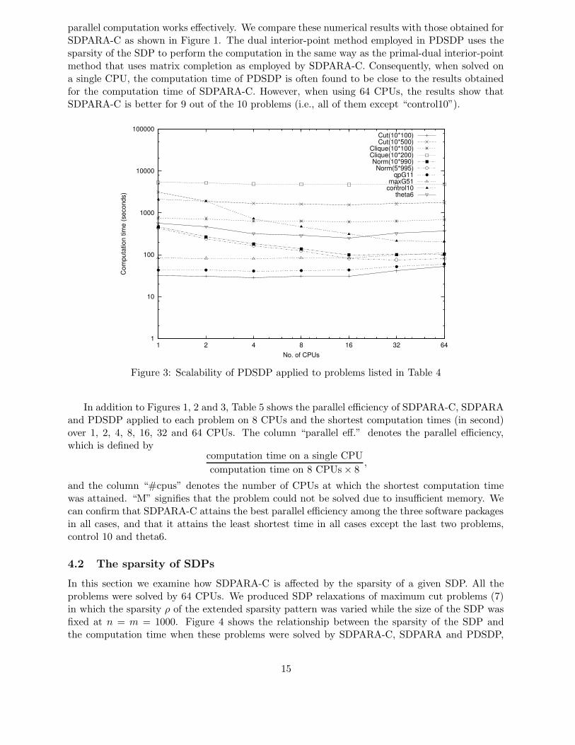
parallel computation works effectively. We compare these numerical results with those obtained forSDPARA-C as shown in Figure 1. The dual interior-point method employed in PDSDP uses thesparsity of the SDP to perform the computation in the same way as the primal-dual interior-pointmethod that uses matrix completion as employed by SDPARA-C. Consequently, when solved ona single CPU, the computation time of PDSDP is often found to be close to the results obtainedfor the computation time of SDPARA-C. However, when using 64 CPUs, the results show thatSDPARA-C is better for 9 out of the 10 problems (i.e., all of them except “control10”).

1

10

100

1000

10000

100000

1 2 4 8 16 32 64

Com

puta

tion

time

(sec

onds

)

No. of CPUs

Cut(10*100)Cut(10*500)


qpG11maxG51

control10theta6

Figure 3: Scalability of PDSDP applied to problems listed in Table 4

In addition to Figures 1, 2 and 3, Table 5 shows the parallel efficiency of SDPARA-C, SDPARAand PDSDP applied to each problem on 8 CPUs and the shortest computation times (in second)over 1, 2, 4, 8, 16, 32 and 64 CPUs. The column “parallel eff.” denotes the parallel efficiency,which is defined by

computation time on a single CPU

computation time on 8 CPUs × 8,

and the column “#cpus” denotes the number of CPUs at which the shortest computation timewas attained. “M” signifies that the problem could not be solved due to insufficient memory. Wecan confirm that SDPARA-C attains the best parallel efficiency among the three software packagesin all cases, and that it attains the least shortest time in all cases except the last two problems,control 10 and theta6.

4.2 The sparsity of SDPs

In this section we examine how SDPARA-C is affected by the sparsity of a given SDP. All theproblems were solved by 64 CPUs. We produced SDP relaxations of maximum cut problems (7)in which the sparsity ρ of the extended sparsity pattern was varied while the size of the SDP wasfixed at n = m = 1000. Figure 4 shows the relationship between the sparsity of the SDP andthe computation time when these problems were solved by SDPARA-C, SDPARA and PDSDP,

15

Table 5: Parallel efficiency on 8 CPUs and shortest computation times for SDPARA-C, SDPARAand PDSDP to solve problems listed in Table 4

SDPARA-C SDPARA PDSDPparallel shortest times parallel shortest times parallel shortest times

Problem eff. (%) sec. #cpus eff. (%) sec. #cpus eff. (%) sec. #cpus

Cut(10*100) 44.9 7.3 32 12.5 160.1 16 13.0 28.1 4Cut(10*500) 90.1 70.7 64 M 24.4 1559.6 16Clique(10*100) 78.8 26.4 64 14.7 224.3 64 14.7 618.6 16Clique(10*200) 73.9 95.6 64 M 13.9 4718.0 16Norm(10*990) 58.1 13.4 32 39.0 407.2 32 41.6 99.8 16Norm(5*995) 46.4 7.1 16 29.6 303.3 32 44.5 76.1 32qpG11 58.9 9.9 32 12.3 650.4 8 12.9 40.9 4maxG51 60.4 56.9 32 12.4 174.6 16 12.5 79.4 4control10 84.5 1034.6 64 71.2 22.0 64 56.1 207.0 64theta6 82.3 101.9 64 77.3 39.1 64 24.0 250.5 16

and Figure 5 shows the relationship between the sparsity of the SDP and the amount of memoryneeded to solve it. In Figures. 4 and 5, the horizontal axis is a logarithmic representation of thesparsity ρ(1 ≤ ρ ≤ 1000), and the vertical axis is a logarithmic representation of the computationtime (or memory usage).

1

10

100

1000

10 100 1000

Com

puta

tion

time(

seco

nds)

Sparsity

SDPARA-CSDPARA

PDSDP

Figure 4: Sparsity and computation time required for SDPARA-C, SDPARA and PDSDP to solveSDP relaxations of maximum cut problems (64 CPUs)

The results in Figure 4 show that as ρ increases, the computation time of SDPARA-C and

16

10

100

1000

10 100 1000

Mem

ory

requ

ired(

MB

)

Sparsity

SDPARA-CSDPARA

PDSDP

Figure 5: Sparsity and memory requirements for SDP relaxations of maximum cut problems bySDPARA-C, SDPARA and PDSDP (64 CPUs)

PDSDP also increases. On the other hand, since SDPARA is implemented without much consid-eration of sparsity of SDPs, the computation time is almost completely independent of the sparsityof an SDP to be solved. The results in Figure 5 show that the memory requirements per processorof SDPARA-C depend on the sparsity of the SDP, whereas the memory requirements per processorof SDPARA and PDSDP remain more or less fixed.

By comparing the results obtained with these three software packages, it can be seen thatSDPARA-C has the shortest computation times and smallest memory requirements when theSDP to be solved is sparse. On the other hand, when the SDP to be solved has little sparsity, theshortest computation times were achieved with SDPARA and the smallest memory requirementswere obtained with PDSDP. The reason why SDPARA-C requires more memory than SDPARAwhen the SDP has less sparsity is because it makes duplicate copies of variables to increase thecomputational efficiency. PDSDP is characterized in that its memory requirements are very lowregardless of how sparse the SDP to be solved is.

4.3 Large-size SDPs

In this section we investigate how large an SDP’s matrix variable can be made before it becomesimpossible for SDPARA-C to solve the problem. In the following numerical experiments, parallelcomputation is performed using all 64 CPUs. The SDPs used in the numerical experiments were theSDP relaxation of a maximum cut lattice graph problem (7), the SDP relaxation of a maximumclique lattice graph problem (8), and a norm minimization problem (9). The size of the SDPrelaxation of the maximum cut problem from a k1 × k2 lattice is n = m = k1k2. As an indicatorof the sparsity of an SDP, we consider the average number ρ of nonzero elements per row of asparse matrix having nonzero elements in the extended sparsity pattern parts. In this problem,ρ ≤ 2min(k1, k2)+1. Therefore, by fixing k1 at 10 and varying k2 from 1000 to 4000, it is possible

17

to produce SDPs with larger matrix variables (i.e., larger n) without increasing the sparsity ρ.Similarly, the size and sparsity of SDP relaxation of maximum clique problems with a k1 × k2

lattice are respectively: n = k1k2, m = 2k1k2 − k1 − k2 + 1, ρ ≤ 2min(k1, k2) + 2. Therefore, byfixing k1 at 10 and varying k2 from 500 to 2000, it is possible to produce SDPs with larger matrixvariables without increasing the sparsity. Also, the size of a norm minimization problem derivedfrom a matrix of size k1 × k2 is n = k1 + k2. When the number of matrices is fixed at 10, m = 11and ρ ≈ 2min(k1, k2) + 1. Therefore, by fixing k1 at 10 and varying k2 from 9990 to 39990, it ispossible to produce SDPs with larger matrix variables without increasing the sparsity; thus ρ ≈ 21for all cases in Table 6.

Table 6: Numerical results on SDPARA-C applied to large-size SDPs (64 CPUs)

time memoryProblem n m (s) (MB)

Cut(10 * 1000) 10000 10000 274.3 126Cut(10 * 2000) 20000 20000 1328.2 276Cut(10 * 4000) 40000 40000 7462.0 720

Clique(10 * 500) 5000 9491 639.5 119Clique(10 * 1000) 10000 18991 3033.2 259Clique(10 * 2000) 20000 37991 15329.0 669

Norm(10 * 9990) 10000 11 409.5 164Norm(10 * 19990) 20000 11 1800.9 304Norm(10 * 39990) 40000 11 7706.0 583

Table 6 shows the computation times and memory requirements per processor needed whenSDPARA-C is used to solve SDP relaxations of maximum cut problems for large lattice graphs,SDP relaxations of maximum clique problems for large lattice graphs and norm minimization prob-lems for large matrices. As one would expect, the computation times and memory requirementsincrease as n gets larger. When n was 2000 or more, SDPARA was unable to solve any of thesethree types of problem due to a lack of memory. Also, PDSDP had insufficient memory to solveSDP relaxations of maximum cut problems with n ≥ 10000 or SDP relaxations of maximum cliqueproblems and norm minimization problems with n ≥ 5000. However, SDPARA-C was able to solveSDP relaxations of maximum cut problems with n = 40000, SDP relaxations of maximum cliqueproblems with n = 20000, and norm minimization problems with n = 40000. Thus in the case ofvery sparse SDPs as solved in this section, solving with SDPARA-C allows an optimal solution tobe obtained to very large-scale SDPs.

4.4 The SDPLIB problems

We performed numerical experiments with a number of problems selected from SDPLIB [7], whichis a set of standard benchmark SDP problems. All the problems were processed in parallel on 8,16 and 32 CPUs. However, in the “equalG11”, “theta6” and “equalG51” problems, the constraintmatrices include a matrix in which all the elements are 1, so these problems were solved aftermaking the transformation proposed in section 6 of the paper [12]. The values of n and m inTable 7 indicate the size of the SDP in the same way as in section 4.1. Also, ρ is an indexrepresenting the sparsity of the SDP as in section 4.3. Cases in which the problem could not besolved due to insufficient memory are indicated as “M”, and cases in which no optimal solutionhad been found after 200 iterations are indicated as “I”.

18

Table 7: Numerical results on SDPARA-C, SDPARA and PDSDP applied to SDPLIB problems

SDPARA-C SDPARA PDSDP# time mem # time mem # time mem

Problem n, m, ρ cpus (s) (MB) cpus (s) (MB) cpus (s) (MB)

thetaG11 801,2401,23 32 95.6 13 32 184.8 159 ImaxG32 2000,2000,32 16 115.5 26 M 8 227.6 58equalG11 801,801,35 32 252.0 115 16 133.1 161 16 258.7 33qpG51 2000,1000,67 32 189.8 83 8 1210.9 955 8 490.5 46control11 165,1596,74 32 2902.5 28 32 124.0 14 32 475.7 20maxG51 1000,1000,134 16 95.2 79 8 173.1 243 8 106.1 18thetaG51 1001,6910,137 32 1870.1 113 M Itheta6 300,4375,271 32 347.3 29 32 188.3 36 8 495.8 37equalG51 1001,1001,534 32 683.3 178 16 241.2 251 16 624.9 51

Table 7 shows the computation times and memory requirements per processor when the short-est computation times are achieved over clusters of 8, 16 and 32 CPUs. We have verified thatSDPARA-C attains higher scalability compared to SDPARA and PDSDP. The SDPs shown inTable 7 are listed in order of increasing sparsity ρ. In cases where the SDP to be solved is sparse(i.e., the problems near the top of Table 7), SDPARA-C was able to reach solutions in the shortestcomputation times and with the smallest memory requirements. In cases where the SDP to besolved is not very sparse (i.e., the problems near the bottom of Table 7), the shortest computationtimes tended to be achieved with SDPARA and the smallest memory requirements tended to beachieved with PDSDP.

4.5 DIMACS

We performed numerical experiments with four problems selected from the 7th DIMACS challenge.All the problems were processed in parallel on 8, 16 and 32 CPUs. Table 8 shows the computationtimes and memory requirements per processor when the shortest computation times are achievedover clusters of 8, 16 and 32 CPUs. Since these problems tend to have optimal solutions with largevalues, we used the starting conditions X = Y = 107I, z = 0. From the results of these numericalexperiments as shown in Table 8, we were able to confirm that the smallest computation timeswere achieved with SDPARA-C, and that the smallest memory requirements were obtained withPDSDP, in cases where the SDP to be solved is large.

Table 8: Numerical results on SDPARA-C, SDPARA and PDSDP applied to DIMACS problems

SDPARA-C SDPARA PDSDP# time mem # time mem # time mem

Problem n, m, ρ cpus (s) (MB) cpus (s) (MB) cpus (s) (MB)

torusg3-8 512,512,78 8 26.4 26 8 46.5 66 8 18.0 7toruspm3-8-50 512,512,78 8 27.5 26 8 53.4 66 8 18.9 7torusg3-15 3375,3375,212 32 826.7 439 M 8 1945.4 159toruspm3-15-50 3375,3375,212 32 866.3 439 M 8 1744.9 159

19

5 Conclusion

In this paper, by applying parallel processing techniques to the primal-dual interior-point methodusing matrix completion theory as proposed in the paper [12, 22], we have developed the SDPARA-C software package which runs on parallel CPUs (PC clusters). SDPARA-C is able to solve large-scale SDPs (SDPs with sparse large-scale data matrices and a large number of linear constraintsin the primal problem (1)) while using less memory. In particular, we have reduced its memoryrequirements and computation time by performing computations based on matrix completiontheory that exploit the sparsity of the problem without performing computations on dense matrices,and by making use of parallel Cholesky factorization. By introducing parallel processing in theparts where bottlenecks have occurred in conventional software packages, we have also succeededin making substantial reductions to the overall computation times.

We have conducted numerical experiments to compare the performance of SDPARA-C withthat of SDPARA [31] and PDSDP [1] in a variety of different problems. From the results of theseexperiments, we have verified that SDPARA-C exhibits very high scalability. We have also foundthat SDPARA-C can solve problems in much less time and with much less memory than othersoftware packages when the extended sparsity pattern is very sparse, and as a result we havesuccessfully solved large-scale problems in which the size of the matrix variable is of the order oftens of thousands – an impossible task for conventional software packages.

As a topic for further study, it would be worthwhile allocating the parallel processing of thecoefficient matrix of the Schur complement equation system proposed in section 3.1 so that theload balance of each CPU becomes more uniform (bearing in mind the need for an allocation thatcan be achieved with a small communication overhead). Numerical experiments have confirmedthat that good results can be achieved even with the relatively simple method proposed in thispaper, but there is probably still room for improvement in this respect.

When solving huge scale SDPs, memory is likely to become a bottleneck. In SDPARA-C, thecoefficient matrix of the Schur complement equation system is partitioned between each CPU, butthe other matrices (including the input data matrix and the sparse factorizations of the matrixvariables in the primal and dual problems) are copied across to and stored on every CPU. Thismemory bottleneck could be eliminated by partitioning each of the matrices copied in this wayand distributing the parts across the CPUs. However, since this would result in greater datacommunication and synchronization overheads, it would probably result in larger computationtimes. Therefore, further study is needed to evaluate the benefits and drawbacks of partitioningthe data in this way.

SDPARA-C has the property of being able to solve sparse SDPs efficiently, and SDPARAhas the property of being able to solve non-sparse SDPs efficiently. In other words, SDPARA-C and SDPARA have a complementary relationship. This fact has been confirmed from thenumerical experiments of section 4.2 and section 4.4. The two algorithms used in SDPARA andSDPARA-C could be combined into a single convenient software package by automatically decidingwhich algorithm can solve a given SDP more efficiently, and then solving the problem with theselected algorithm. To make this decision, it would be necessary to estimate the computation timesand memory requirements of each algorithm. However, estimating computation times in parallelprocessing is not that easy to do.

Acknowledgment

The authors thank to two anonymous referees for their many suggestions and comments whichconsiderably improved the paper.

20

References

[1] S.J. Benson, Parallel Computing on Semidefinite Programs, Preprint ANL/MCS-P939-0302,http://www.msc.anl.gov/˜benson/dsdp/pdsdp.ps (2002).

[2] S.J. Benson, Y. Ye and X. Zhang, Solving large-scale sparse semidefinite programs for com-binatorial optimization, SIAM Journal on Optimization, 10 (2000) 443–461.

[3] A. Ben-Tal, M. Kocvara, A. Nemirovskii and J. Zowe, Free material optimization via semidef-inite programming: the multiload case with contact conditions, SIAM Journal on Optimiza-tion, 9 (1999) 813-832.

[4] A. Ben-Tal and A. Nemirovskii, Lectures on Modern Convex Optimization Analysis, Algo-rithms, and Engineering Applications, SIAM, Philadelphia (2001).

[5] L.S. Blackford, J. Choi, A. Cleary, E. D’Azevedo, J. Demmel, I. Dhillon, J. Dongarra, S Ham-marling, G. Henry, A. Petitet, K. Stanley, D. Walker and R.C. Whaley, ScaLAPACK Users’Guide, SIAM, Philadelphia (1997).

[6] B. Borchers, CSDP 2.3 user’s guide, Optimization Methods and Software, 11 & 12 (1999)597–611. Available at http://www.nmt.edu/˜borchers/csdp.html.

[7] B. Borchers, SDPLIB 1.2, a library of semidefinite programming test problems, OptimizationMethods and Software, 11 & 12 (1999) 683-690.

[8] S. Burer, Semidefinite programming in the space of partial positive semidefinite matrices,SIAM Journal on Optimization, 14 (2003) 139-172.

[9] S. Burer, R.D.C. Monteiro, and Y. Zhang, A computational study of a gradient-based log-barrier algorithm for a class of large-scale SDPs, Mathematical Programming, 95 (2003) 359–379.

[10] C. Choi and Y. Ye, Solving sparse semidefinite programs using the dual scaling algorithm withan iterative solver, Manuscript, Department of Management Sciences, University of Iowa, IowaCity, IA 52242 (2000).

[11] K. Fujisawa, M. Kojima and K. Nakata, Exploiting sparsity in primal-dual interior-pointmethods for semidefinite programming, Mathematical Programming, 79 (1997) 235–253.

[12] M. Fukuda, M. Kojima, K. Murota and K. Nakata, Exploiting sparsity in semidefinite pro-gramming via matrix completion I: General framework, SIAM Journal on Optimization, 11(2000) 647–674.

[13] D.R. Fulkerson and J.W.H. Gross, Incidence matrices and interval graphs, Pacific Journal ofMathematics, 15 (1965) 835–855.

[14] D. Goldfarb and G.Iyengar, Robust portfolio selection problems, Mathematics of OperationsResearch, 28 (2003) 1–38.

[15] W. Gropp, E. Lusk and A. Skjellum, Using MPI: Portable Parallel Programming with theMessage-Passing Interface, MIT Press, Massachusetts (1994).

[16] C. Helmberg and F. Rendl, A spectral bundle method for semidefinite programming, SIAMJournal on Optimization, 10 (2000) 673–696.

21

[17] C. Helmberg, F. Rendl, R. J. Vanderbei and H. Wolkowicz, An interior-point method forsemidefinite programming, SIAM Journal on Optimization, 6 (1996) 342–361.

[18] M. Kocvara and M. Stingl, PENNON - A Code for Convex Nonlinear and Semidefinite Pro-gramming, Optimization Methods and Software, 18 (2003) 317–333.

[19] M. Kojima, S. Shindoh and S. Hara, Interior-point methods for the monotone semidefinitelinear complementarity problem in symmetric matrices, SIAM Journal on Optimization, 7(1997) 86–125.

[20] R. D. C. Monteiro, Primal-dual path-following algorithms for semidefinite programming,SIAM Journal on Optimization, 7 (1997) 663–678.

[21] R. D. C. Monteiro, First- and second-order methods for semidefinite programming, Mathe-matical Programming, 97 (2003) 209–244.

[22] K. Nakata, K. Fujisawa, M. Fukuda, M. Kojima and K. Murota, Exploiting sparsity in semidef-inite programming via matrix completion II: Implementation and numerical results, Mathe-matical Programming, 95 (2003) 303–327.

[23] K. Nakata, K. Fujisawa and M. Kojima, Using the conjugate gradient method in interior-pointmethods for semidefinite programs (in Japanese), Proceedings of the Institute of StatisticalMathematics, 46 (1998) 297–316.

[24] M. Nakata, H. Nakatsuji, M. Ehara, M. Fukuda, K. Nakata and K. Fujisawa, Variationalcalculations of fermion second-order reduced density matrices by semidefinite programmingalgorithm, Journal of Chemical Physics, 114 (2001) 8282-8292.

[25] J. F. Sturm, Using SeDuMi 1.02, a MATLAB toolbox for optimization over symmetric cones,Optimization Methods and Software, 11 & 12 (1999) 625–653.

[26] K. C. Toh and M. Kojima, Solving some large scale semidefinite programs via conjugateresidual method, SIAM Journal on Optimization, 12 (2002) 669–691.

[27] K. C. Toh, M. J. Todd and R. H. Tutuncu, SDPT3 — a MATLAB software package forsemidefinite programming, version 1.3, Optimization Methods and Software, 11 & 12 (1999)545–581. Available at http://www.math.nus.edu.sg/˜mattohkc.

[28] H. Waki, S. Kim, M. Kojima and M. Muramatsu, Sums of squares and semidefinite program-ming relaxations for polynomial optimization problems with structured sparsity, ResearchReport B-411, Department of Mathematical and Computing Sciences, Tokyo Institute ofTechnology, Meguro, Tokyo 152-8552 (2005).

[29] H. Wolkowicz, R. Saigal and L. Vandenberghe, eds., Handbook of Semidefinite Programming,Theory, Algorithms, and Applications, Kluwer Academic Publishers, Massachusetts (2000).

[30] M. Yamashita, K. Fujisawa and M. Kojima, Implementation and Evaluation of SDPA6.0(SemiDefinite Programming Algorithm 6.0), Optimization Methods and Software, 18 (2003)491–505.

[31] M. Yamashita, K. Fujisawa and M. Kojima, SDPARA: SemiDefinte Programming AlgorithmPARAllel version, Parallel Computing, 29 (2003) 1053–1067.

22

a parallel primal-dual interior-point method for semide …kojima/articles/b-398.pdfa parallel...

Documents