a parallel algorithm for constrained two-staged two-dimensional cutting problems

Computers & Industrial Engineering 62 (2012) 177–189

Contents lists available at SciVerse ScienceDirect

Computers & Industrial Engineering

journal homepage: www.elsevier .com/ locate/caie

A parallel algorithm for constrained two-staged two-dimensionalcutting problems q

Mhand Hifi a,⇑, Stephane Negre a, Rachid Ouafi b, Toufik Saadi a

a Université de Picardie Jules Verne, Unité de Recherche EPROAD, 5 rue du Moulin Neuf, 80000 Amiens, Franceb Université de Technologie Houari-Boumediene, LAID3, El Alia, BP 32, Bab Ezzouar, 16111 Alger, Algeria

a r t i c l e i n f o

Article history:Available online 16 September 2011

Keywords:Beam-searchDynamic programmingHeuristicsKnapsackMaster–slave paradigmOptimization

0360-8352/$ - see front matter � 2011 Elsevier Ltd. Adoi:10.1016/j.cie.2011.09.005

q This paper is part of the Special Issue CombinatorEngineering.⇑ Corresponding author.

E-mail address: [email protected] (M. Hifi).

a b s t r a c t

In this paper, we solve the two-staged two-dimensional cutting problem using a parallel algorithm. Theproposed approach combines two main features: beam search (BS) and strip generation solution proce-dures (SGSP). BS employs a truncated tree-search, where a selected subset of generated nodes are retunedfor further search. SGSP, a constructive procedure, combines a (sub)set of strips for providing both partiallower and complementary upper bounds. The algorithm explores in parallel a subset of selected nodesfollowing the master–slave paradigm. The master processor serves to guide the search-resolution andeach slave processor develops its proper way, trying a global convergence. The aim of such an approachis to show how the parallelism is able to efficiently solve large-scale instances, by providing new solu-tions within a consistently reduced runtime. Extensive computational testing on instances, taken fromthe literature, shows the effectiveness of the proposed approach.

� 2011 Elsevier Ltd. All rights reserved.

1. Introduction

In this paper, we investigate the use of a parallel algorithm for avariant of the two-dimensional cutting problem (TDC). An instanceof TDC problem is characterized by a single rectangular stock sheetS of dimensions L �W and a set I = {1, . . . ,n} of n type pieces whereeach type i 2 I has a profit ci. We say that the n-dimensional vector(x1, . . . ,xn) of integer and nonnegative numbers corresponds to acutting pattern, if it is possible to produce xi pieces of type i,i = 1, . . . ,n, in the large stock rectangle S without overlapping. TheTDC consists of determining the cutting pattern with themaximum value, i.e.,

TDC ¼max

Pni¼1

cixi

subject to ðx1; . . . ; xnÞ corresponds to a cutting pattern:

8<:

ð1Þ

In TDC one has, in general, to satisfy a certain demand of pieces. Theproblem is called unconstrained if these demand values are notimposed, and constrained if the demand is represented by a vectorb = (b1, . . . ,bn), where bi is the maximum number of times that pieceof type i, i = 1, . . . ,n, can appear in a cutting pattern. Another variantof the TDC problem is to consider a constraint on the total number

ll rights reserved.

ial Optimization in Industrial

of cuts, i.e., the sum of some parallel vertical and/or horizontal cuts(using guillotine cuts) does not exceed a certain nonnegative inte-ger k <1. In this case, the problem is called the k � staged TDC(or kTDC) problem (see Gilmore & Gomory, 1965; Hifi & Roucairol,2001). We distinguish two versions of the TDC problem: the un-weighted version in which the profit ci = li � wi, "i 2 I, and theweighted version in which the profit of each piece can be indepen-dent to its area, i.e., $ i 2 I such that ck – liwi. Herein, we also assumethat (i) pieces have fixed orientation; that is, pieces of dimensions(‘,x) and (x,‘) are different, and (ii) all cutting tools are of guillotinetype, i.e., the vertical and the horizontal cuts produce two sub-rectangles.

In this paper, we propose a parallel algorithm, which is an ex-tended version of the paper exposed in Hifi, Negre, and Saadi(2009). According to the definition of the kTDC, we study the casefor which k = 2; that is, the problem in which each piece is obtainedby two guillotine cuts (as illustrated in Fig. 1a):

(i) R is first divided into a set of horizontal strips, and(ii) each generated horizontal strip is subsequently considered

individually and chopped across its width.

Note that the two-stage guillotine pattern of Fig. 1a is withouttrimming since no additional cutting stage is required to extracteach piece. On the other hand, the two-stage guillotine pattern ofFig. 1b is with trimming since an additional cutting stage isnecessary for extracting some of the pieces (Alvarez-Valdes, Martı,Parajón, & Tamarit, 2007; Gilmore & Gomory, 1965; Hifi &

http://dx.doi.org/10.1016/j.cie.2011.09.005

mailto:[email protected]

http://dx.doi.org/10.1016/j.cie.2011.09.005

http://www.sciencedirect.com/science/journal/03608352

http://www.elsevier.com/locate/caie

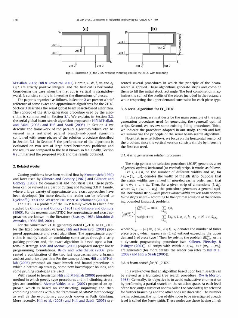
Fig. 1. Illustration (a) the 2TDC without trimming and (b) the 2TDC with trimming.

178 M. Hifi et al. / Computers & Industrial Engineering 62 (2012) 177–189

M’Hallah, 2005; Hifi & Roucairol, 2001). Herein, L, W, li, wi and bi,i 2 I, are strictly positive integers, and the first cut is horizontal.Considering the case when the first cut is vertical is straightfor-ward. It consists simply in inverting the dimensions of pieces.

The paper is organized as follows. In Section 2 we present a briefreference of some exact and approximate algorithms for the 2TDC.Section 3 describes the serial global beam search-based algorithm.The concept of the strip generation procedure used by the algo-rithm is summarized in Section 3.1. We explain, in Section 3.2,the serial global beam-search algorithm proposed in Hifi, M’Hallah,and Saadi (2008) and Hifi and Saadi (2005). In Section 4 wedescribe the framework of the parallel algorithm which can beviewed as a restricted parallel branch-and-bound algorithmcombined with some phases of the solution procedure describedin Section 3.1. In Section 5 the performance of the algorithm isevaluated on two sets of large sized benchmark problems andthe results are compared to the best known so far. Finally, Section6 summarized the proposed work and the results obtained.

2. Related works

Cutting problems have been studied first by Kantorovich (1960)and later used by Gilmore and Gomory (1961) and Gilmore andGomory (1965), for commercial and industrial uses. These prob-lems can be viewed as a part of Cutting and Packing (C& P) family,where a large variety of approximate and exact approaches havebeen developed (for more details, the reader can be refereed toDyckhoff (1990) and Wäscher, Haussner, & Schumann (2007)).

The 2TDC is a problem of the C& P family which has been firststudied by Gilmore and Gomory (1961) and Gilmore and Gomory(1965). For the unconstrained 2TDC, few approximate and exact ap-proaches are known in the literature (Beasley, 1985; Morabito &Arenales, 1996; Hifi, 2001).

For the constrained 2TDC (generally noted C_2TDC or FC_2TDCfor the fixed orientation version), Hifi and Roucairol (2001) pro-posed approximate and exact algorithms. The approximate algo-rithm is mainly based on combining some strips through a strippacking problem and, the exact algorithm is based upon a bot-tom-up strategy. Lodi and Monaci (2003) proposed integer linearprogramming formulations. Belov and Scheithauer (2006) pre-sented a combination of the two last approaches into a branchand cut and price algorithm. For the same problem, Hifi and M’Hal-lah (2005) proposed an exact branch and bound procedure inwhich a bottom-up strategy, some new lower/upper bounds, andsome pruning strategies are used.

With regard to heuristics, Hifi and M’Hallah (2006) presented amethod in which greedy type procedures and hill climbing strate-gies are combined. Alvarez-Valdes et al. (2007) proposed an ap-proach which is based on constructing, improving and thencombining solutions within the framework of GRASP methodologyas well as the evolutionary approach known as Path Relinking.More recently, Hifi et al. (2008) and Hifi and Saadi (2005) pre-

sented several procedures in which the principle of the beam-search is applied. These algorithms generate strips and combinethem to fill the initial stock rectangle. The best combination max-imizes the sum of the profits of the pieces included in the rectanglewhile respecting the upper demand constraint for each piece type.

3. A serial algorithm for FC_2TDC

In this section, we first describe the main principle of the stripgeneration procedure, used for generating the (general) optimalstrips. Second, we review some existing filling procedures. Third,we indicate the procedure adapted in our study. Fourth and last,we summarize the principle of the serial beam-search algorithm.

Note that, in what follows, we focus on the horizontal version ofthe problem, since the vertical version consists simply by invertingthe first-cut used.

3.1. A strip generation solution procedure

The strip generation solution procedure (SGSP) generates a setof general optimal horizontal (or vertical) strips. It works as follows.

Let s, s 6 n, be the number of different widths and �wj, forj 2 J = {1, . . . ,s}, denotes the width of the jth strip. Suppose thatthe strips widths are ranked in non-decreasing order such that�w1 < �w2 < . . . < �ws. Then, for a given strip of dimensions ðL; �wjÞ,where �wj 2 fw1; . . . ;wng, the procedure generates a general opti-mal horizontal strip �with pieces whose widths are less than or equalto the strip’s width� according to the optimal solution of the follow-ing bounded knapsack problem:

BKhorL; �wj

� � f hor�wjðLÞ ¼max

Pi2SL; �wj

cixij

subject toP

i2SL; �wj

lixij 6 L; xij 6 bi; xij 2 N; i 2 SL; �wj;

8>><>>:

where SðL; �wjÞ ¼ fk j wk 6 �wj; k 2 Ig: xij denotes the number of timespiece type i, which appears in ðL; �wjÞ without exceeding the upperdemand bi of piece type i. Then, by solving the problem BKhor

L; �ws, using

a dynamic programming procedure (see Kellerer, Pferschy, &Pisinger (2003)), all strips with width x 6 �ws; x 2 f�w1; . . . ; �wsg,are generated (for more details, the reader can refer to Hifi et al.(2008) and Hifi & Saadi (2005)).

3.2. A beam-search for FC _2 TDC

It is well-known that an algorithm based upon beam search canbe viewed as a truncated tree search procedure (Ow & Morton,1988). Generally, its objective is to avoid exhaustive enumerationby performing a partial search on the solution space. At each levelof the tree, only a subset of nodes (called the elite nodes) are selectedfor further branching and the other ones are discarded. The numberx characterizing the number of elite nodes to be investigated at eachlevel is called the beam width. These nodes are those having a high

M. Hifi et al. / Computers & Industrial Engineering 62 (2012) 177–189 179

potential to lead to the optimal solution. The potential of each nodeis assessed using an evaluation operator, and so for sake clarity, wesummarize in this section the Serial Global Beam Search (SGBS) pro-posed in Hifi et al. (2008) and Hifi and Saadi (2005). First, we intro-duce the definition of the nodes of the tree and the branchingmechanism out of the nodes of the main list, namely B (as describedin the algorithm of Fig. 2). Second and last, we describe the mainsteps of the SGBS algorithm considered in our study.

3.2.1. Applying BS to FC_2TDCApplying beam search to FC_2TDC requires (i) defining the

nodes of the tree and, (ii) the branching mechanism.On the one hand, a node can be considered as a pair of sub-rect-

angles (L,W � Y) and (L,Y), Y 6W. The first sub-rectangle (L,W � Y)is characterized by its local partial feasible solution reached by thesuccessive combinations of strips, and (L,Y) is the complementarysub-rectangle that remains to be filled. Using such a definition, weobserve that the root node can be characterized by a pair of sub-rectangles (L,0) and (L,W) because no strip has been packed intothe rectangle (L,W).

On the other hand, branching out of a (selected) nodel = ((L,W � Y), (L,Y)), Y 6W, is equivalent to packing a strip(L,b),b 6 Y, b 2 {w1, . . . ,wn}, into the sub-rectangle (L,Y). There willbe at most r branches emanating out of node l, such that r 6 s.Each resulting node corresponds to packing a strip ðL; �wjÞ; j 2J :¼ f1; . . . ; rg and each of these created nodes will be representedby the pair of sub-rectangles ððL;W � Y þ �wjÞ; ðL;Y � �wjÞÞ; j 2 J.

Two cases can be distinguished when applying SGBS. Indeed,the strips being appended when branching out of a node are gen-erated as follows (it also depends on the construction used):

Fig. 2. A serial global beam-search (S

� At the root node, no strip has been packed; thus b0i ¼ bi; 8i 2 I.The algorithm creates r:¼s distinct general optimal stripsðL; �wjÞ; j 2 J, by applying SGSP to the largest knapsack problemBKg

L; �wr. Each selected strip j 2 J corresponds to a branch emanat-

ing from the root node and leads to a newly created nodeððL; �wjÞ; ðL;W � �wjÞÞ; j 2 J.� To branch out of an internal node ((L,W � Y), (L,Y)), SGBS algo-

rithm considers the following steps:

0
1. Compute the residual demand bi for each piece type i, i 2 I,where b0i ¼ bi � v i with vi being the number of times piecetype i appears in (L,W � Y).
2. For j = 1, . . . ,r, apply SGSP on the problem BKgL;�wj

.3. For each strip ðL; �wjÞ; j ¼ 1; . . . ; r, and �wj 6 Y ,

(a) pack the strip into the current sub-rectangle (L,Y),(b) obtain a new node l ¼ ððL;W � Y þ �wjÞ; ðL;Y � �wjÞÞ, and(c) assess the values zLocal

l and zGloball of the new node (as

defined below: Section 3.2.2).

3.2.2. A serial global beam-searchThe serial global beam-search (SGBS) (described in Fig. 2) is a

beam search using a total-cost evaluation operator. It selects thenode having the best potential of leading to the optimal solution.Its operator assesses the potential zGlobal

l of a node l = ((L,W � Y),(L,Y)), Y 6W, of B, by combining what follows:

(i) zLocall , the value of the partial feasible solution associated

with (L,W � Y), and(ii) UðL;YÞ, an upper bound for the value of the complementary

sub-rectangle (L,Y).

GBS) for the FC_2TDC problem.


An upper bound UðL;YÞ for the profit, generated by filling (L,Y), isthe optimal solution value of the following knapsack problem:

UKðL;YÞ ¼maxXj2J

f g�wjðLÞtj j

Xj2J

�wjtj 6 Y; tj 2 N; j 2 J

( ); ð2Þ

where f g�wjðLÞ is the profit of the general optimal strip ðL; �wjÞ obtained

by applying SGSP to BKgL; �wj

with b0i ¼ bi � v i; i 2 I (vi is, as previouslydefined, the number of times piece type i appears in the partial fea-sible solution associated with (L,W � Y)). The integer variable tj isthe number of occurrences of the general strip ðL; �wjÞ in (L,Y). Thevalue UðL;YÞ is provided when solving the problem UK(L, Y). In fact, be-cause UðL;YÞ is an upper bound, it can be computed only once at theroot node with b0i ¼ bi and its value used throughout the search tree.Indeed, solving the aforementioned knapsack via dynamic program-ming yields all upper bounds UðL;YÞ corresponding to all possiblesub-rectangles (L,Y), with Y = 0,1, . . . ,W. Thus, at each node of thedeveloped tree, an upper bound corresponding to the current sub-rectangle (L,Y) is available; that is UðL;YÞ.

In order to accelerate and to manage the search process, twocriteria can be used. One way of accelerating the search is to reducethe space search by fathoming any new node l = ((L,W � Y), (L,Y)),such that Y 6W, of B, whose

zGloball ¼ zLocal

l þ UðL;YÞ 6 z�; ð3Þ

where zq is the solution value of the current incumbent solution.Another way, which serves to guide the search of the promising

paths, is to define from B the best potential value C such that

C ¼maxl2B

zGloball

n o: ð4Þ

In addition, for each l 2 B, the gap between zLocall and C is evaluated.

Then, the min{d, jBj} nodes, with largest gaps, are selected.

4. A parallel global beam-search algorithm

In this section, we first discuss the phases which seem parallel-izable. Second, we present the design consideration of the algo-rithm. Third, we focus on the data structures used: we discussthe global list associated with master processor and two internaland complementary lists associated with each slave processor.Fourth and last, we summarize the principle of the parallelalgorithm.

4.1. How exploiting parallelism

An examination of the serial algorithm SGBS (cf., Fig. 2) revealsthe potential for exploiting parallelism when solving the problem.The runtime occurs when applying the following phases:

1. The selection phase: the choice is performed for selecting thebest promising node.

2. The expanding phase: first, all general optimal strips are cre-ated for each width’s strip (they are obtained by solving aseries of knapsack problems �cf., Section 3.1�). Second, allupper bounds are computed in order to evaluate the poten-tial of the nodes. These bounds correspond to the optimalvalues of the generated sub-rectangles (they are obtainedby combining the optimal strips according to the rest ofthe sub-rectangle to fill �cf., Eq. (2)�).

3. The filtering phase:it serves to select a subset of the promisingnodes.

We observe that the processing, which corresponds to the threephases described above, can be distributed, thereby dividing the

computational work among a number of processors. In order toadopt such an approach, we use a parallel approach, which consistsin exploring in parallel g nodes of the developed tree according tothe master–slave paradigm (see Vairaktarakis, 1997). Herein, themaster processor serves to guide the search-resolution by main-taining a global list of nodes which were not explored; it uses abest-first search strategy for selecting the successive sets of elitenodes. Whereas each slave processor develops the search treeand updates the list of the master processor in an asynchronousmanner (for a detailed study on parallel branch-and-bound, thereader can refer to Crainic, Le Cun, & Roucairol (2006), Gendron& Crainic (1994) and Grama, Kumar, & Pardalos (1993)).

4.2. Design consideration

One of the challenges in efficiently parallelizing the FC_2TDC isthat the amount of runtime processing done, in both selecting andcomputing/expanding steps, is highly variable. Also, in some casessuch a runtime processing becomes unpredictable. Indeed, on theone hand, the selection phase can be performed by using a list con-taining the nodes sorted following a specified order. On the otherhand, the expanding phase consumes the majority of the runtime,because (i) it creates – at each selection – all the distinct generaloptimal strips, (ii) it performs a global evaluation according to bothupper bound and partial feasible solution, and (iii) it updates thebest internal solution. In addition, the amount of the function thatcan be generated by the filtering phase may be unpredictable. Thisnecessitates that any approach to parallelization must incorporatemechanisms for dynamic load balancing.

The proposed parallel algorithm works as follows:

1. From the global list B �managed by the master processor�, asubset of nodes is selected and assigned to the availableslave processors.

2. Each slave processor uses its proper internal lists for evaluat-ing the process corresponding to the selection, the expand-ing and the filtering phases.

3. The algorithm employs a load balancing protocol for keepingthe resolving process balanced. For each slave processor, itis realized by using a threshold n limiting the size of the firstinternal list and considers a secondary internal list for limitingthe number of local nodes to be considered. Then, if the limitimposed is reached, the slave processor transfers all ele-ments of the secondary list to the master processor in anasynchronous manner.

4. In addition, periodically the algorithm uses a runtime limit,namely T, for reinitializing the internal lists associated tothe slave processors. In this case, the restarting process canbe applied in a synchronous manner.

In what follows, we recall that from a selected node l =((L,W � Y), (L,Y)) emerges r, r 6 s, different offsprings ((L,W � Y +x), (L,Y �x)), where x ¼ �w1; . . . ; �wr . For each generated nodem, a partial lower bound zLocal

m and a complementary upper boundUðL;Y�xÞ are needed for evaluation the future paths to expand; thus,the filtering phase takes place.

4.3. Representation and process managing

SGBS considers three complementary phases: the selection, theexpanding and the filtering phases. The parallel version of the algo-rithm explores in parallel a subset of selected nodes following themaster–slave paradigm. The master processor guides the searchprocess by using a special list recording a variety of nodes to devel-op. The slave processor (i) develops the way of the search, (ii)updates the special list maintained by the master processor in an


asynchronous manner and (iii) considers a periodic runtime in or-der to restart the slave processor in a synchronous manner.

4.3.1. Using internal and global listsThe master processor (cf. Fig. 3) localizes the nodes recorded into

a special list, called global list and denoted Bmaster. Such a list is alsoused for starting the parallel search: it is considered for creatingthe first s nodes characterizing the widths �wj; j 2 J. Each widthwj, j 2 J characterizes a strip with width wj having a partial feasiblesolution reached by applying SGSP to the largest knapsack problemBKhor

L; �ws; s 6 jJj (cf., Section 3.1).

Each available slave processor (cf. Fig. 3) receives an initial nodel = ((L,W � Y), (L,Y)), from the master processor, where l is com-posed of its residual width Y and the number vi, i = 1, . . . ,n, of timesthat the ith piece appears in the partial feasible solution of valuezLocall . The slave processor uses two internal lists: (i) the first internal

list (denoted Bslave), which serves to stock the best generated nodes,following the best-first search strategy, and (ii) the second internallist (denoted Bslave), which is considered for storing the remainingnodes when the first internal list Bslave is full. Herein, the full listis represented by its maximum capacity and for Bslave its size isdenoted nslave :¼ nBslave

. Of course, in our study we used the samesize-internal-list for all slave processors; that is n = nslave, forslave = 1, . . . ,g which represents its maximal cardinality.

Then, for a given node l = ((L,W � Y), (L,Y)) belonging to Bslave,the slave processor starts its processing, which is based on the fol-lowing steps:

1. It computes the residual demand b0i for each piece type i, i 2 I,where b0i = bi � vi with vi being the number of times piecetype i appears in (L,W � Y).

2. It creates the r (r 6 s 6 n) general strips by applying SGSP toBKg

L; �wr, where r ¼ arg maxf �wr j �wr P �wj; j 2 Jg.

3. For each strip ðL; �wjÞ; �wj 6 Y; j ¼ 1; . . . ; r, do:(a) pack the strip into the current sub-rectangle (L,Y),(b) obtain a new node m ¼ ððL;W � Y þ �wjÞ; ðL;Y � �wjÞÞ, and(c) assess the value zm of the new node.

We observe that SGBS considers a local list Bd (cf., Fig. 2, the fil-tering phase of the iterative step), which serves to store all the in-duced nodes from a selected node, namely l. For the parallelversion, we propose to replace the list with Bslave. In this case, froma selected node l 2 Bslave, all generated nodes are first stored intothe secondary internal list Bslave. Second, the best nodes belongingto Bslave are transferred to the first internal list Bslave. Third and last,the residual nodes of Bslave are transferred to the master list Bmaster.

Because there exists r different widths, then r new local nodesare generated. Thus, the filtering phase is applied in order to selectthe eligible paths corresponding to the elite nodes. These nodes arethose realizing the minfd; jBslavejg best gaps (as defined in Eqs. (3)and (4), Section 3.2.2), where d denotes the beam width.

Fig. 3. Illustration of the master processor and both internal lists associated to theslave processors.

4.3.2. The jumping strategyWe recall that each slave processor obtains a work from its local

work list Bslave. A processor’s local work serves to modify the inter-nal lists when both expanding and filtering phases are active.Whenever a slave processor runs out of work, it either sends a sub-set of created nodes Bslave or transfers the whole nodes ofBslave [ Bslave to the master processor. According to the case consid-ered, the algorithm reacts as follows:

1. On the one hand, sending the nodes of Bslave, from the slaveprocessor to the master one, means that the size n of the firstinternal list Bslave is reached. Then, the master processorreceives the nodes and retains only the nodes whose globalevaluations remain larger than the best evaluation zq.

2. On the other hand, transferring the nodes of Bslave [ Bslave

means that a limit runtime T is used for stopping the pro-cessing of the whole slave processors in a synchronous man-ner. Then, each slave processor sends the nodes and the bestlocal solution found so far.

For the case (1), the algorithm applies load balancing for allslave processors. It introduces, for each slave processor, a thresholdn limiting the size of the first internal list. For the case (2), it uses ajumping strategy in order to diversify the search space. Indeed, themaster processor considers the following steps before sending thebest selected nodes to the available g slave processors:

1. It updates the best feasible solution provided by the slaveprocessors and replaces Bmaster with Bmaster [

Pgslave¼1Bslave[Pg

slave¼1Bslave.2. It applies a filtering phase for reducing the number of nodes

belonging to the global list Bmaster.3. It selects the min{g,jBmasterj} nodes using a best-first strategy

and affects them to the slave processors.4. It removes the assigned nodes from the global list Bmaster.

4.4. The components of the parallel approach

The parallel version of SGBS is based on the master algorithm,the slave algorithm and how to manage the communications andwaiting times between all the processors.

4.4.1. The master algorithmFig. 4 describes the main steps used by the master processor,

noted Master_Algo. It is composed of three steps: the initializa-tion, the synchronization and the terminal steps.

The initialization step serves to initialize the global list Bmaster

(step 1. (a)) to the starting node l:¼((L,0), (L,W)) and to buildthe first s distinct general optimal strips by solving the problemBKhor

L; �ws(step 1. (b)). The aforementioned problem denotes the larg-

est knapsack because �ws is the highest width; thus, solving it witha dynamic programming procedure (i.e. calling the solution proce-dure SGSP) induces all the general optimal strips whose widths are�wj 6 �ws; j 2 J :¼ f1; . . . ; sg, with their values f hor

�wj. Second, in step 1.

(c), according to the couples �wj; f hor�wj

� �; j 2 J, the (complementary)

upper bounds are computed by solving the knapsack problemUK(L, W) using a dynamic programming procedure. Third, in step1. (d), a first filtering phase is used on the s created nodes: (i) the

best solution value zq is updated by maxj2J zLocalj

n o; and (ii) the

structure realizing the upper bound UðL;YÞ is transformed in orderto remove the non-feasibility of the solution. Fourth, in step 1.(e), a global vector Active is used for controlling the state of theslave processors; each slave processor k has its component Activek,which is equal to false if the processor is available, true

Fig. 4. The global procedure used by the master processor: Master_Algo.


otherwise. Initially, all components are equal to false since allslave processors are in standby. Fifth and last, in step 1. (f), themaster processor selects the a best nodes following the best-firstsearch strategy; they are the nodes realizing the best global evalu-ation zGlobal

j ¼ zLocalj þ UðL;W��wjÞ; j 2 J, and assigns them to the slave

processor, i.e., Slave_Algo lk;Bk;Bk; T� �

; k ¼ 1; . . . ;a, where lk isthe k-th selected node from Bmaster, Bk and Bk denote both internallists associated to the k-th slave processor and T is the periodicruntime limit.

The synchronization step is composed of three cases and themaster processor reacts according to the encountered case. Forthe first case, a number, namely P0 6 P, of slave processors sendtheir residual nodes to the master processor (we recall that theresidual nodes are those of the secondary internal list Bslave). The

master processor receives these P lists (step 2.1. (a)) and it mergestheir nodes to the global list Bmaster (step 2.1. (b)). It then, in step2.1. (c), applies a filtering phase which serves to eliminate theduplicate nodes and the nodes whose global evaluations are lessthan or equal to the value zq (of course, in this case, the masterprocessor updates the best solution if necessary).

For the second case, a slave processor, namely k, terminates itsprocessing. So, the master processor (step 2.2. (a)) receives the con-text representing the best solution produced with its structure.Then, it replaces the status of the slave processor by false and up-dates the best solution if necessary. Second, in step 2.2. (b), the fil-tering phase is applied on the global list if and only if the bestsolution has been improved; in this case, each node having a globalevaluation smaller than zq is removed from Bmaster. Third and last

1 www.grid5000.fr.


(step 2.2. (c)), the master processor selects the best node, namelyl, belonging to the global list Bmaster by using the best-first searchstrategy and it assigns the node l to an available slave processor.

For the third case, all slave processors are stopped because theperiodic runtime limit T is consumed. First, in step 2.3. (a), themaster processor receives all the nodes of the active slave proces-sors, namely P0 6 P, corresponding to the nodes [P0

k¼1Bk[P0k¼1Bk: Sec-

ond, it switches in step 2.3. (b) the status of P0 slave processorsfrom true to false and it merges (step 2.3. (c)) the nodes of[P0

k¼1Bk[P0k¼1Bk to the global list Bmaster. Third, in step 2.3. (d), it up-

dates the best solution zq and applies a filtering phase on theresulting global list Bmaster. Fourth and last, in step 2.3. (e), the mas-ter processor assigns the best a nodes to the available slave proces-sors when Bmaster – ;.

The terminal step serves to stop the master processor with thebest solution with value zq. In fact, the master processor stopsthe processing when all components of the vector Active have thevalue false, which means that all the slave processors have termi-nated the processing and all message-queues of the master proces-sor are empty (the message-queues and the communicationprocesses are detailed in Section 4.4.3).

4.4.2. The slave algorithmFig. 5 describes the main steps of the algorithm, noted Sla-

ve_Algo, used by each slave processor k, k = 1, . . . ,P, where P de-notes the number of the available slave processors. The resultingalgorithm resembles to SGBS detailed in Fig. 2 with some modifica-tions. Indeed, as shown in Fig. 5, the algorithm is composed ofthree steps: the initialization, the iterative and the stopping condi-tion steps.

In the initialization step, the slave processor receives the node lassigned by the master processor, with its residual demandb0i; i 2 I. Then, in step 1.1, the node is stored in the first internal listBk and in step 1.2, r new distinct general optimal strips are createdwhose widths are �wj; j 2 J and with objective values f hor

�wj; j 2 J.

These strips are obtained by considering SGSP applied to the fol-lowing knapsack problem (solved with a dynamic programmingprocedure):

BKhorL;�wj

� �ghor

�wjðLÞ ¼max

Pi2SL; �wj

cixij

subject toP

i2SL; �wj

lixij 6 L

xij 6 b0i; xij 2 N; i 2 SL;�wj;

8>>>>><>>>>>:

where �wr 6W �Wl and ghor�wjðLÞ is the objective value of the created

general optimal strip of width �wj; j 2 J :¼ f1; . . . ; rg. Furthermore,all complementary upper bounds are computed by solving, with adynamic programming, the following knapsack problem:

UKðL;WlÞ ¼ maxXj2J

gg�wjðLÞtj j

Xj2J

�wjtj 6W �Wl; tj 2 N; j 2 J

( ):

The iterative step starts (step 2.1) by selecting the best node,namely l = ((L,W � Y), (L,Y)), of the first internal list Bk and re-moves it from this list (step 2.2). Second, in step 2.3, r(r 6 s 6 n)general optimal strips are builded by solving BKg

L;�wr, where

r ¼ arg maxf�wr j �wr P �wj; �wj 6Wl; j 2 Jg. Third, in step 2.4, foreach created node m both lower bound (i.e., zLocal

m ) and complemen-tary upper bound (i.e., Um) are updated for evaluating the valuezGlobalm ; that is the potential of the node m for a future selection.

Fourth, steps 2.5 makes a selection on the generated nodes andtransfers them to the secondary list Bk while step 2.6 considers afiltering phase on Bk by retuning the best minfd; jBkjg nodes realiz-ing better global evaluations (according to Eq. (4)). Fifth and last,step 2.7 verifies if the number of available nodes (i.e., Bk [ Bk) is

less than or equal to the threshold n (i.e., the size of the first inter-nal list Bk); if the last case happens, a part of nodes of Bk are trans-ferred to Bk and the residual nodes are transferred to the masterprocessor. Moreover, in both cases the secondary internal list Bk

is reduced to an empty set.The stopping condition step is composed of two parts. For the

first part, in step 3.1, the slave processor stops the processingeither if Bk is reduced to an empty set or if the periodic runtimelimit T is consumed. On the one hand, if the first internal list Bk

is empty, then the slave processor sends the best solution obtainedand it informs the master processor by setting Activek = false. Onthe other hand, if the periodic runtime T is attained, then the bestsolution value reached, the nodes of both internal lists (i.e. Bk andBk) and Activek with the value false are transferred to the masterprocessor. Otherwise, for the second part, the iterative step isrecalled.

4.4.3. Communications and waiting timesThe communications between the master and slave processors

are established according to three queues. Each queue is managedby a process which exploits the information transferred by theslave processors. Herein, the received information may representeither the best local solution or the subset of nodes. According tothe queue considered, the information is stored following the FIFOstrategy. The role of the three queues is explained in what follows.

During the resolution process, the first queue (noted Q1 inFig. 6) is used for storing the best local solutions transferred bythe slave processors. In fact, it corresponds to the synchronizationphase of Algo_Master when a slave processor sends a solution toQ1. The second queue (noted Q2 in Fig. 6) serves to receive theresidual nodes transferred by the slave processors. In this case, itcorresponds to Case 1 of the synchronization step of Algo_Master.The third queue (noted Q3 in Fig. 6) is considered for load balanc-ing; i.e., it serves to stock the nodes emanated from the slave pro-cessors and to redistribute them to the available slave processors.

Note that, on the one hand, the treatment of the three queues isdone in an independent manner. Differently stated, the treatmentsof the various cases associated to the synchronization step (cases1–3) are done in parallel. One the other hand, for each periodicruntime T�characterizing the synchronization point�, the lasttwo queues (after the filtering stage) are reduced to empty queues.

5. Computational results

In this section, we investigate the effectiveness of the parallelalgorithm, noted PGBS, on two set of instances taken from the lit-erature (all instances are extracted from Alvarez-Valdes et al.(2007), Hifi et al. (2008) and Hifi & M’Hallah (2006)). The first setis composed of 22 large instances and the second one containssix more hardness instances. PGBS runs under Linux heteroge-neous workstations of the GridD5000 plate-form1 (for more details,the reader can refer to BEA (2007), BEA (2007) and Walker & Don-garra (1996) for message-passing programming principles and com-munication queue management).

Generally, when using approximate algorithms to solve optimi-zation problems, it is well-known that different parameter settingsfor the approach lead to results of variable quality. As discussed inHifi et al. (2008), the value assigned to the beam width d varies inthe discrete interval {1, . . . ,4}, and for the serial algorithm, a highervalue for d does not necessary gives better solutions but the run-time may become more important. In what follows, we will discussthe behavior of PGBS on all instances and we will compare its pro-vided results to the best solutions taken from the literature. The

http://www.grid5000.fr

Fig. 5. Description of the steps used by the kth slave processor.

Fig. 6. Illustration of the message-queues used by the master processor.


analysis of these aspects considers different levels of d; thus, forseveral values of d, each instance is run using both SGBS and PGBS.

5.1. The first set of instances

We first tested the algorithm on the twenty-two large-scale in-stances extracted from Alvarez-Valdes et al. (2007), Hifi et al.(2008), and Hifi and Saadi (2005). Each instance was run twice:the first run corresponds to the version of the problem when thefirst cut is made horizontally and the second run represents the sec-ond version when the first cut is made vertically (the name of theinstance terminates respectively with H and V for the horizontaland vertical versions of the problem). There are several instancesfor which the optimal solutions are unknown; thus, the solutionreached by PGBS is compared to the best solution taken from theliterature (cf., Hifi et al., 2008. On the other hand (as mentionedin Hifi et al. (2008)), regarding that SGBS has difficult to solvelarge-scale instances with a high value of the beam width, we thenopted for stopping the runtime after 300 s (if the algorithm does


not terminate before the considered limit). Note that even if theaforementioned limit can seem restrictive for this set of instances,such a choice can be considered as a way to study and to analyzethe behavior of the parallel algorithm compared with that of thesequential. Of course, for the more hardness instances (see Section5.2), we shall see the behavior of the sequential algorithm with andwithout limiting the runtime.

The analysis of the obtained results for the first set on instancesfollows. Table 1 reports the computational results for the 22 large-sized instances. Column 1 refers to the instance number and col-umn 2 contains either the optimal solution Opt if known or thebest known solution from the literature (whenever the optimalsolution is known, the instance is marked with the symbol ‘‘⁄’’).Columns 3 and 5 show respectively the gap, noted Gap, of the solu-tion obtained by SGBS with the beam width d = 4 and d = 8, respec-tively. Columns 4 and 6 tally the runtime that needs PGBS forreaching its best solutions for both values of d. Columns 7–10 dis-play the results of PGBS with a beam width d = 8: column 7 reportsPGBS’s gap and columns 8, 9 and 10 display respectively the run-

Table 1Computational results of PGBS versus SGBS. The symbol ‘‘�’’ means that SGBS exceeds talgorithm matches the best solution from the literature.

#Inst. Opt/Best SGBS Algorithm

d = 4 d = 8

Best cpu Best

nice25H⁄ 860,829 860,829 0.05 860,829nice50H 913,738 913,738 0.01 913,738nice100H 911,122 911,122 0.05 911,122nice200H 931,143 931,143 0.41 919,756nice500H 951,279 951,279 1.86 935,467path25H⁄ 892,765 892,765 0.06 892,765path50H⁄ 750,215 750,215 0.05 750,215path100H 888,578 888,578 0.08 888,611path200H 889,174 889,174 1.59 879,921path500H 885,112 885,112 12.87 870,912nice25PH⁄ 441,993 441,993 0.02 441,993nice50PH 449,292 449,292 0.02 449,292nice100PH 456,306 456,306 0.05 448,732nice200PH 455,727 455,727 0.16 455,701nice500PH 455,036 455,036 1.44 435,733nice1000PH 451,805 451,805 2.94 430,003path25PH⁄ 464,721 464,721 0.01 464,721path50PH 391,626 391,626 0.01 390,741path100PH 456,300 456,300 0.09 428,798path200PH 452,402 452,402 1.34 419,704path500PH 434,478 434,478 40.52 412,731path1000PH 434,966 434,966 150.21 424,961

nice25V⁄ 834,157 834,157 0.01 834,157nice50V 854,425 854,425 1.12 854,425nice100V 911,958 911,958 3.41 890,571nice200V 935,290 935,290 4.55 909,906nice500V 960,767 960,767 10.54 929,871path25V⁄ 699,707 699,707 0.01 699,707path50V⁄ 924,908 924,908 0.41 924,908path100V⁄ 754,678 754,678 3.43 744,671path200V 836,022 836,022 3.56 815,807path500V 798,544 798,544 4.54 767,912nice25PV⁄ 428,662 428,662 0.13 428,662nice50PV 425,921 425,921 0.55 425,921nice100PV 451,851 451,851 0.43 429,180nice200PV 454,754 454,754 1.23 423,964nice500PV 457,381 457,381 10.41 407,301nice1000PV 459,142 459,142 3.44 439,142path25PV⁄ 356,088 356,088 0.05 356,088path50PV 487,447 487,447 0.11 487,447path100PV 386,033 386,033 1.23 386,033path200PV 418,024 418,024 2.34 406,656path500PV 368,284 368,284 5.2 329,989path1000PV 407,097 407,097 77.54 377,882

Av_Gap 0.00 �12221.52Av_cpu 7.91

times that needs PGBS for reaching its best solution. Note thatthe gap denotes the difference between the solution reached bythe considered algorithm and Opt/Best; in this case, Gap > 0 meansthat the corresponding algorithm improves the best solution fromthe literature. The last section (i.e., the last two rows) of Table 1provides a summary of the results. It displays the average gap,noted Av_Gap and the average computational time, noted Av_cpu,over all instances.

First, from Table 1, we observe what follows:SGBS4 matches all the best solutions from the literature (44 in-

stances representing 22 instances for H and 22 instances for V). Itsaverage computational time is equal to 7.91 s, which can be con-sidered as a reasonable average runtime for a sequential algorithm.

SGBS8 has a worse behavior compared to SGBS4. Indeed, as dis-cussed in Hifi et al. (2008) and Hifi & Saadi (2005), this phenome-non can be explained by the fact that the runtime limit of 300 sremains insufficient for the serial algorithm with a beam widthd = 8. Thus, on the one hand, this version of the algorithm matches16 out of 44 instances (representing a percentage of 36.36%) and

he fixed runtime limit of 300 s and we use the symbol ‘‘�’’ when the corresponding

PGBS Algorithm (d = 8)

P = 6 P = 10 P = 20

cpu Best cpu cpu cpu

7.76 860,829 0.02 0.01 023.87 913,738 0.01 0.01 0� 911,122 0.01 0.01 0.01� 940,040 0.21 0.11 0.01� 953,598 1.01 0.09 0.04

17.76 892,765 0.02 0.01 0.01105.21 750,215 0.02 0.01 0.01� 888,578 0.01 0.01 0.01� 890,223 0.98 0.43 0.21� 887,664 12.91 6.76 4.245.65 441,993 0.01 0.01 0

21.87 449,292 0.01 0.01 0� 456,306 0.01 0.01 0.01� 456,888 0.09 0.03 0.01� 459,001 1.33 0.78 0.69� 459,076 2.08 0.59 0.49

10.78 464,721 0.01 0.01 089.09 391,626 0.01 0.01 0� 457,997 0.21 0.02 0� 459,856 0.99 0.45 0.12� 440,167 36.79 25.08 12.99� 440,001 99.99 69.77 19.61

9.32 834,157 0.01 0.01 0.0122.98 854,425 0.86 0.45 0.23� 911,958 2.04 1.48 0.89� 935,290 2.44 1.99 0.99� 965,604 6.89 3.98 1.987.91 699,707 0.01 0 0.00

29.07 924,908 0.32 0.13 0.03� 758,695 2.78 1.87 0.76� 836,022 2.81 2.05 1.99� 799,903 2.45 1.42 0.72

10.87 428,662 0.02 0.01 0.0131.67 425,921 0.34 0.21 0.01� 455,406 0.21 0.11 0.01� 454,754 1.08 0.99 0.69� 457,381 7.76 3.67 2.03� 459,142 2.02 1.32 0.95

12.67 356,088 0.02 0.01 0.0132.73 487,447 0.04 0.02 0.01� 386,033 0.65 0.42 0.21� 422,705 1.56 0.43 0.22� 368,284 3.06 2.88 1.04� 409,823 40.76 22.76 13.76

1551.45200.89 5.34 3.42 1.48


degrades the other solutions with an average gap of �12221.52. Onthe other hand, the Av_cpu considerably increases which becomesnow equal to 200.89 s on average.

PGBS8 performs better than both versions of SGBS. Indeed, itimproves in 17 out of 44 instances (representing 38.6% of theweighted and unweighted cases) and matches the remaining bestsolutions from the literature. Note that over the rest of theinstances, PGBS8 matches 11 optimal solutions.

Let PGBSP8 be the version of the parallel algorithm using P proces-

sors, S(P) be the speedup and F(P) its efficiency. Thus, depending onthe number of processors used, the analysis is commented asfollows:

1. The average runtime of PGBS68 is much smaller than the

7.91 s average runtime of SGBS4 and the 200.89 s of theSGBS8. According to the best average runtime realized bySGBS4, PGBS6

8 decreases the average computational time of86.3%. In this case, the speedup S(6) and the efficiency F(6)is respectively equal to 1.48 and 0.25 respectively.

2. The average runtime of PGBS108 diminishes of 35.9% com-

pared to PGBS86’s average runtime. In this case, the speedup

S(10) and the efficiency F(10) become respectively equal to2.31 and 0.23 respectively.

3. PGBS208 ’s average runtime is more interesting. Indeed, it

decreases from 3.42 s (according to PGBS108 ’s average run-

time) to 1.48 s. In this case, the diminution becomes moreimportant compared to the best serial version of the algo-rithm, i.e., it decreases of 81.20% on average. Moreover, thespeedup S(20) and the efficiency F(20) are respectively equalto 5.34 and 0.27 respectively.

According to the above analysis, on the one hand, we observethat S(6) represents almost the half of S(10), S(10) representsalmost the half of S(20) and the three values F(6), F(10) andF(20), which measure the efficiency of the algorithm, are mostequivalent. Note also that the comparison of the performance ofPGBS for weighted versus unweighted is inconclusive. In some in-

Table 2Behavior of PGBS when varying the periodic runtime limit T.

T = 0.5 s T = 1 s

P = 6 P = 10 P = 20 P = 6

Av_Nj 16.44 9.99 6.02 8.77Av_cpu 24.99 17.73 8.38 5.34nbBest/Opt 44 44 44 44

Table 3Performance of the parallel algorithm on the second set of instances.

#Inst. Best Cplex HESGAb SGBS

d = 2 d = 4

Best cpu Best

UL1H 887,393 876,682 887,099 887,393 138.56 1,074,752UL2H 906,237 900,923 906,237 906,237 310.13 1,122,376UL3H 1,017,575 1,009,031 1,017,575 1,017,575 347.89 1,036,385WL1H 688,840 687,786 688,840 688,840 410.09 857,621WL2H 782,566 778,028 782,566 782,566 454.76 907,702WL3H 899,890 897,373 899,890 899,890 488.76 1,386,291UL1V 891,516 888,762 891,516 891,516 120.87 575,432UL2V 908,982 906,600 908,982 908,982 210.41 678,751UL3V 1,022,483 1,018,888 1,018,888 1,022,483 320.87 897,651WL1V 694,657 694,657 694,657 694,657 340.89 516,709WL2V 783,836 782,149 782,149 783,836 410.78 490,765WL3V 881,931 881,931 881,931 881,931 456.81 609,875

Av_Gap �3591.33 �464.67 0.00 �218070.67Av_cpu 334.24

stances, the weighted problems are solved faster while in other in-stances they are harder to solve.

We have already mentioned that PGBS uses a periodic runtime Tfor synchronizing all the slave processors (cf, Section 4.3.2). It canbe considered as a diversification strategy, which serves to exploremore regions of the feasible search space. In fact, the results re-ported in Table 2 are obtained by fixing T to one seconds,. The con-sidered choice was decided after several tunings. Indeed, thecomputational results were conducted by varying the value of Tfrom 0.5 s to 2 s with a path of 0.5, and we only retained the threesignificant values as shown in Table 2: line 1 displays the numberof average jumping (Av_Nj), line 2 tallies the average runtime(Av_cpu) that needs each algorithm for terminating and line 3 re-ports the number (nbBest/Opt) of times that the current version of thealgorithm matches the new solutions.

Let PGBSP8ðTÞ be the parallel algorithm executed with the param-

eters P (number of processors), T (the value associated to the peri-odic runtime) and the beam with d = 8. The analysis of the results ofTable 2 revels that PGBSP

8ðT ¼ 1Þ, for P = 6,10 and 20, has a betterbehavior than the other versions of the algorithm. Indeed, first, bothPGBSP

8ð0:5Þ and PGBSP8ð1Þ match all the 44 best solutions, but

PGBSP8ð1Þ seems slightly faster than PGBSP

8ð0:5Þ. Second, only 38or 39 out of 44 instances are matched by PGBSP

8ð2Þ, but its averageruntime remains globally more interesting. Third and last, we cannotice that PGBSP

8ð1Þ remains more favorable than PGBSP8ð2Þ be-

cause the average computational time function of the number ofbetter obtained solutions is more advantageous for PGBSP

8ð1Þ; inthis case, PGBSP

8ð1Þ realizes an average runtime-unit varying from1.48 to 5.34 whereas PGBSP

8ð2Þ realizes its value from 2.62 to 4.55.

5.2. The second set of instances

In this section, for the second set of instances which contains sixmore hardness instances (noted LU1, LU2, LU3, LW1, LW2 andLW3, respectively), we maintain the version of PGBS with T = 1.Since no optimal solution is known for these instances, we thencompared the solution obtained by PGBS to the best solutions

T = 2 s

P = 10 P = 20 P = 6 P = 10 P = 20

6.01 2.99 5.88 3.23 1.883.42 1.48 4.55 3.66 2.6244 44 38 39 39

SGBSfull PGBS (d = 4)

d = 4 P = 6 P = 10 P = 20

cpu Best cpu Best cpu cpu cpu

} 700,034 8240.6 887,393 139.99 120.66 102.76} 690,098 7865.03 907,866 240.87 201.87 180.77} 998,765 7791.66 1,100,992 229.77 194.27 174.61} 520,059 7654 694,099 301.87 266.06 207.03} 657,430 5671.12 784,128 299.25 243.44 208.06} 413,489 5071.22 899,890 334.98 301.55 281.55} 575,432 8753.12 900,099 101.87 92.09 86.01} 678,751 6542 910,021 195.67 174.65 109.07} 897,651 6120.09 1,027,491 222.98 206.98 190.65} 516,709 5991.9 699,994 270.65 209.11 191.08} 490,765 5764.02 783,836 299.65 267.99 241.04} 609,875 5997.99 892,650 399.04 307.99 281.77

�218070.67 10212.75900.00 6788.56 253.04 215.55 187.86

Tabl

e4

Perf

orm

ance

ofPG

BS:

the

runt

ime

cons

umed

byof

each

proc

esso

r.

#In

st.

PGB

S:Pa

rall

elG

loba

lB

eam

Sear

chSG

BS

wit

hd

=4

d=

4M

axim

um

run

tim

eP

=6

P=

10P

=20

Bes

tSo

luti

on

P=

6P

=10

P=

20M

in.

Av.

Max

.M

in.

Av.

Max

.M

in.

Av.

Max

.M

ax.

Av.

Min

.

UL1

H88

7,39

313

9.99

120.

6610

2.76

99.0

613

4.07

137.

9998

.09

117.

0311

9.09

98.7

699

.54

100.

0088

2,03

288

2,03

2–

UL2

H90

7,86

624

0.87

201.

8718

0.77

190.

6423

7.01

239.

8719

5.00

197.

4320

0.00

170.

0079

.09

178.

0089

9,19

689

9,19

6–

UL3

H1,

100,

992

229.

7719

4.27

174.

6120

0.54

222.

5522

5.09

186.

5419

0.51

192.

0016

0.54

171.

4317

3.43

1,01

3,79

9–

–W

L1H

694,

099

301.

8726

6.06

207.

0320

0.32

297.

3229

9.42

250.

0926

0.65

264.

4319

0.00

200.

4420

5.00

666,

162

––

WL2

H78

4,12

829

9.25

243.

4420

8.06

210.

0729

7.42

299.

0822

0.41

241.

0024

2.01

196.

0020

1.43

205.

55–

––

WL3

H89

9,89

033

4.98

301.

5528

1.55

250.

0929

8.09

300.

0127

0.00

296.

0930

0.00

169.

0127

4.05

279.

53–

––

UL1

V90

0,09

910

1.87

92.0

986

.01

86.0

698

.33

99.6

688

.65

89.7

690

.42

65.0

582

.42

84.4

189

1,51

689

1,51

689

1,51

6U

L2V

910,

021

195.

6717

4.65

109.

0719

0.08

192.

6519

4.56

164.

0717

1.09

173.

5489

.01

103.

3210

6.32

908,

982

908,

982

908,

982

UL3

V1,

027,

491

222.

9820

6.98

190.

6519

9.41

217.

0921

9.08

198.

0920

0.00

204.

3218

0.00

185.

4218

7.42

1,02

2,48

31,

022,

483

–W

L1V

699,

994

270.

6520

9.11

191.

0824

5.54

263.

5126

5.22

195.

0020

3.06

207.

4317

4.32

185.

3218

8.01

697,

164

697,

164

–W

L2V

783,

836

299.

6526

7.99

241.

0428

0.08

293.

5329

6.01

240.

4426

1.33

265.

4320

7.00

224.

0023

8.42

783,

836

––

WL3

V89

2,65

039

9.04

307.

9928

1.77

386.

8839

4.44

396.

0928

7.01

301.

0030

5.43

261.

4327

6.42

279.

0189

0,69

6–

–

Av.

253.

0421

5.55

187.

8621

9.89

253.

8325

6.01

199.

4521

0.75

213.

6816

3.68

178.

5718

5.43


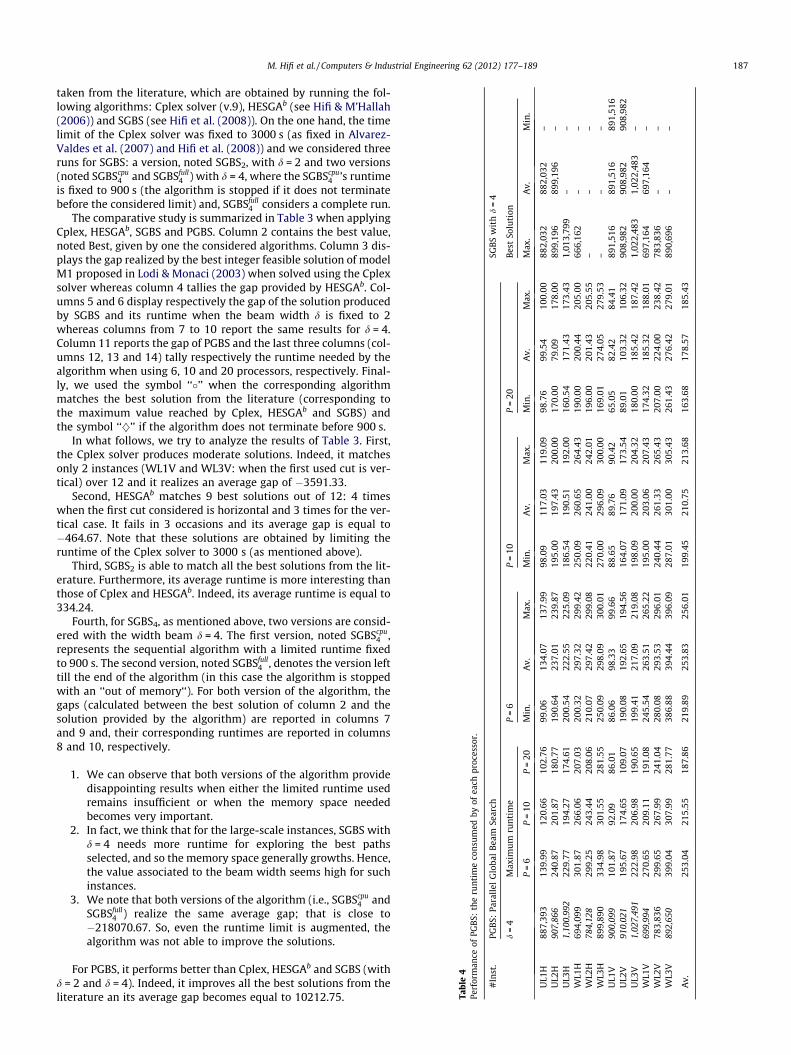
taken from the literature, which are obtained by running the fol-lowing algorithms: Cplex solver (v.9), HESGAb (see Hifi & M’Hallah(2006)) and SGBS (see Hifi et al. (2008)). On the one hand, the timelimit of the Cplex solver was fixed to 3000 s (as fixed in Alvarez-Valdes et al. (2007) and Hifi et al. (2008)) and we considered threeruns for SGBS: a version, noted SGBS2, with d = 2 and two versions(noted SGBScpu

4 and SGBSfull4 ) with d = 4, where the SGBScpu

4 ’s runtimeis fixed to 900 s (the algorithm is stopped if it does not terminatebefore the considered limit) and, SGBSfull

4 considers a complete run.The comparative study is summarized in Table 3 when applying

Cplex, HESGAb, SGBS and PGBS. Column 2 contains the best value,noted Best, given by one the considered algorithms. Column 3 dis-plays the gap realized by the best integer feasible solution of modelM1 proposed in Lodi & Monaci (2003) when solved using the Cplexsolver whereas column 4 tallies the gap provided by HESGAb. Col-umns 5 and 6 display respectively the gap of the solution producedby SGBS and its runtime when the beam width d is fixed to 2whereas columns from 7 to 10 report the same results for d = 4.Column 11 reports the gap of PGBS and the last three columns (col-umns 12, 13 and 14) tally respectively the runtime needed by thealgorithm when using 6, 10 and 20 processors, respectively. Final-ly, we used the symbol ‘‘�’’ when the corresponding algorithmmatches the best solution from the literature (corresponding tothe maximum value reached by Cplex, HESGAb and SGBS) andthe symbol ‘‘}’’ if the algorithm does not terminate before 900 s.

In what follows, we try to analyze the results of Table 3. First,the Cplex solver produces moderate solutions. Indeed, it matchesonly 2 instances (WL1V and WL3V: when the first used cut is ver-tical) over 12 and it realizes an average gap of �3591.33.

Second, HESGAb matches 9 best solutions out of 12: 4 timeswhen the first cut considered is horizontal and 3 times for the ver-tical case. It fails in 3 occasions and its average gap is equal to�464.67. Note that these solutions are obtained by limiting theruntime of the Cplex solver to 3000 s (as mentioned above).

Third, SGBS2 is able to match all the best solutions from the lit-erature. Furthermore, its average runtime is more interesting thanthose of Cplex and HESGAb. Indeed, its average runtime is equal to334.24.

Fourth, for SGBS4, as mentioned above, two versions are consid-ered with the width beam d = 4. The first version, noted SGBScpu

4 ,represents the sequential algorithm with a limited runtime fixedto 900 s. The second version, noted SGBSfull

4 , denotes the version lefttill the end of the algorithm (in this case the algorithm is stoppedwith an ‘‘out of memory‘‘). For both version of the algorithm, thegaps (calculated between the best solution of column 2 and thesolution provided by the algorithm) are reported in columns 7and 9 and, their corresponding runtimes are reported in columns8 and 10, respectively.

1. We can observe that both versions of the algorithm providedisappointing results when either the limited runtime usedremains insufficient or when the memory space neededbecomes very important.

2. In fact, we think that for the large-scale instances, SGBS withd = 4 needs more runtime for exploring the best pathsselected, and so the memory space generally growths. Hence,the value associated to the beam width seems high for suchinstances.

3. We note that both versions of the algorithm (i.e., SGBScpu4 and

SGBSfull4 ) realize the same average gap; that is close to

�218070.67. So, even the runtime limit is augmented, thealgorithm was not able to improve the solutions.

For PGBS, it performs better than Cplex, HESGAb and SGBS (withd = 2 and d = 4). Indeed, it improves all the best solutions from theliterature an its average gap becomes equal to 10212.75.

Table 5Performance of PGBS on the second set of instances: runtime consumed by the Master processor and the load balancing cost.

Runtime Runtime Runtime and Load Balancing CostPGBS with d = 4 runtime Av. Slave proc. Av. Master proc.Nb. Processors Nb. Processors Nb. Processors

#Inst. 6 10 20 6 10 20 6 10 20

UL1H 134.07 120.66 102.76 134.07 117.03 99.54 5.92 3.63 3.22UL2H 237.01 201.87 180.77 237.01 197.43 79.09 3.86 4.44 101.68UL3H 222.55 194.27 174.61 222.55 190.51 171.43 7.22 3.76 3.18WL1H 297.32 266.06 207.03 297.32 260.65 200.44 4.55 5.41 6.59WL2H 297.42 243.44 208.06 297.42 241.00 201.43 1.83 2.44 6.63WL3H 298.09 301.55 281.55 298.09 296.09 274.05 36.89 5.46 7.50UL1V 98.33 92.09 86.01 86.06 89.76 82.42 15.81 2.33 3.59UL2V 192.65 174.65 109.07 192.65 171.09 103.32 3.02 3.56 5.75UL3V 217.09 206.98 190.65 217.09 200.00 185.42 5.89 6.98 5.23WL1V 263.51 209.11 191.08 263.51 203.06 185.32 7.14 6.05 5.76WL2V 293.53 267.99 241.04 293.53 261.33 224.00 6.12 6.66 17.04WL3V 394.44 307.99 281.77 394.44 301.00 276.42 4.60 6.99 5.35

Av_cpu 253.04 215.55 187.86 253.83 210.75 178.57 8.57 4.81 14.29% Balancing 1.15 2.27 1.90


Concerning its runtime, the analysis is made following the num-ber of the processors used:

1. The average runtime of PGBS64ð1Þ is much smaller than the

253.04 s average runtime of SGBS2, the 900 seconds ofSGBScpu

4 and the 3000 s of the Cplex solver.(a) According to the SGBS2’s average runtime, PGBS6

4ð1Þdecreases the average runtime of 24.3%. Moreover, onthe one hand, its speedup S(6) and its efficiency F(6) arerespectively equal to 1.32 and 0.22 respectively.

(b) According to the average runtimes of both versions ofSGBS with d = 4 (i.e., SGBScpu

4 and SGBSfull4 ), PGBS6

4ð1Þ real-izes a more interesting average runtime, even the secondversion SGBSfull

4 was stopped because of the importantmemory space needed. In this case, when comparing thefirst version, i.e., SGBScpu

4 , PGBS64ð1Þ’s speedup S(6) and

its efficiency F(6) are respectively equal to 3.56 and 0.59respectively.

2. PGBS104 ð1Þ’s average runtime decreases of 35.5% regarding

the PGBS68ð1Þ’s average runtime.

(a) On the one hand, the speedup S(10) and the efficiencyF(10) become respectively equal to 1.55 and 0.16respectively.

(b) On the other hand, when considering SGBScpu4 ;PGBS6

4ð1Þ’sspeedup S(6) and its efficiency F(6) are respectively equalto 4.18 and 0.42 respectively.

3. PGBS204 ð1Þ’s average runtime is more interesting. Indeed, in

this case, it decreases from 215.55 s (according toPGBS10

4 ð1Þ’s average runtime) to 187.86 s. Note that the dim-inution becomes more important compared to the best serialversion of the algorithm, i.e., its decreases of 43.7% onaverage.

(a) On the one hand, its S(20) and F(20) are respectively equalto 1.78 and 0.09 respectively.

(b) On the other hand, when using d = 4 i.e.,SGBS4; PGBS6

4ð1Þ’s speedup S(6) and its efficiency F(6)are respectively equal to 4.79 and 0.24 respectively.

5.3. PGBS versus SGBS

In order to evaluate the impact of the the parallel approach, wedecided to compare the results produced by both approaches(SGBS and PGBS) with varying the final runtime consumed. Be-cause the parallel version of the algorithm is tailored for hardnessinstances, we just considered the second set of instances. For these

instances, we first considered the runtime realized by PGBS whenvarying the number of slave processors (reported in Table 4, col-umns from 2 to 4) and we selected among all runtimes consumedby the used slave processors, three significant ones: the minimumruntime (noted Min_cpu), the average runtime (noted Av_cpu), themaximum runtime (noted Max_cpu). The three aforementionedvalues are reported in Table 4 following the number of slave pro-cessors used: columns from 6 to 8 with 6 processors, columns from9 to 11 with 10 processors and columns from 12 to 14 with 20 pro-cessors. Second, SGBS was run with the three aforementioned val-ues and the results reached by the algorithm are reported in Table4 (the three last columns). Third and last, from Table 4, we observethat the quality of solutions reached by SGBS are very far to thoseproduced by the parallel version PGBS. According to the compara-tive study, we can also show the interesting effect induced by thediversification phase used by the parallel algorithm. Moreover,using the parallel version PGBS becomes more interesting, sinceit is able to produce better solutions than those produced by SGBSand without any problem of storage memory.

Another interesting point, when applying parallel approaches, isto study the impact of the cost induced by the load balancingbetween the processors. Herein, we exploited the results of Table 4for evaluating the percentage value during the resolution searchconsidered by the parallel beam search. From these values, weextracted the runtime dedicated to the load balancing used by themaster processor. Table 5 summarizes these results: as shown fromTable 5, globally only 2% of the global runtime of PGBS is assignedfor the load balancing. Indeed, such a percentage varies from1.15% (with 6 slave processors) to 2.27% (with 20 slave processors).

6. Conclusion

This paper solves the constrained two-staged two-dimensionalcutting problem using a parallel global beam search. The algorithmcan be viewed as a truncated branch-and-bound where only a sub-set of nodes are investigated. It is based in exploring on parallelsome elite nodes, selected following a best-first search strategy,according to the master–slave paradigm. The computational inves-tigation shows that the parallel global beam search outperformsthe serial version and other existing algorithms for two sets ofinstances varying from large to very-large ones. It yields optimalsolutions for some large problems and improves the majority ofthe best known solutions taken from the literature.


References

Alvarez-Valdes, R., Martı, R., Parajón, A., & Tamarit, J. M. (2007). GRASP and pathrelinking for the two-dimensional two-staged cutting stock problem. INFORMSJournal on Computing, 19, 1–12.

BEA (2007). MessageQ, programming guide. BEA Corporation.BEA (2007). MessageQ, Introduction to Message Queuing. BEA Corporation.Beasley, J. E. (1985). Algorithms for unconstrained two-dimensional guillotine

cutting. Journal of the Operational Research Society, 36, 297–306.Belov, G., & Scheithauer, G. (2006). A branch-and-cut-and-price algorithm for one-

dimensional stock cutting and two-dimensional two-stage cutting. EuropeanJournal of Operational Research, 171(1), 85–106. 1985.

Crainic, T. G., Le Cun, B., & Roucairol, C. (2006). Parallel branch-and-boundalgorithms. In E-G. Talbi (Ed.), Parallel combinatorial optimization. Wiley.ISBN:978-0-471-72101-7.

Dyckhoff, H. (1990). A typology of cutting and packing problems. European Journal ofOperational Research, 44, 145–159.

Gendron, B., & Crainic, T. G. (1994). Parallel branch-and-bound algorithms: Surveyand synthesis. Operations Research, 42(6), 1042–1066.

Gilmore, P. C., & Gomory, R. E. (1961). A linear programming approach to the cuttingstock problem. Operations Research, 9, 849–859.

Gilmore, P. C., & Gomory, R. E. (1965). Multistage cutting problems of two and moredimensions. Operations Research, 13, 94–119.

Grama, A., Kumar, V., & Pardalos, P. (1993). Parallel processing of discrete optimizationproblems. Encyclopedia of Microcomputers. John Wiley & Sons.

Hifi, M. (2001). Exact algorithms for large-scale unconstrained two and three stagedcutting problems. Computational Optimization and Applications, 18, 63–88.

Hifi, M., Negre, S., & Saadi, T. (2009). A parallel algorithm for constrained fixed two-staged two-dimensional cutting/packing problems. In IEEE/CIE39: Proceedings ofthe international conference on computers & industrial engineering (pp. 328–330).Troyes, France, 6–9 July (2009).

Hifi, M., M’Hallah, R., & Saadi, T. (2008). Algorithms for the constrained two-stagedtwo-dimensional cutting problem. INFORMS Journal on Computing, 20, 212–221.

Hifi, M., & M’Hallah, R. (2006). Strip generation algorithms for two-staged two-dimensional cutting stock problems. European Journal of Operational Research,172, 515–527.

Hifi, M., & M’Hallah, R. (2005). An exact algorithm for constrained two-dimensionaltwo-staged cutting problems. Operations Research, 53, 140–150.

Hifi, M., & Roucairol, C. (2001). Approximate and exact algorithms for constrained(un)weighted two-dimensional two-staged cutting stock problems. Journal ofCombinatorial Optimization, 5, 465–494.

Hifi, M., & Saadi, T. (2005). Using strip generation procedures for solvingconstrained two-staged cutting problems. In The fifth ALIO/EURO conference oncombinatorial optimization. Paris, France: ENST.

Kantorovich, L. V. (1960). Mathematical methods of organizing and planningproduction. Management Science, 6, 363–422.

Kellerer, H., Pferschy, U., & Pisinger, D. (2003). Knapsack problems. Springer.Lodi, A., & Monaci, M. (2003). Integer linear programming models for 2-staged two-

dimensional knapsack problems. Mathematical Programming, 94, 257–278.Morabito, R., & Arenales, M. (1996). Staged and constrained two-dimensional

guillotine cutting problems: An and–or-graph approach. European Journal ofOperational Research, 94(3), 548–560.

Ow, P. S., & Morton, T. E. (1988). Filtered beam search in scheduling. InternationalJournal of Production Research, 26, 297–307.

Vairaktarakis, G. (1997). Analysis of algorithms for master-slave system. IEEETransactions, 29(11), 39–949.

Walker, D. W., & Dongarra, J. J. (1996). MPI: A standard message passing interface.Supercomputer, 12, 56–68.

Wäscher, G., Haussner, G., & Schumann, H. (2007). An improved typology of cuttingand packing problems. European Journal of Operational Research, 183,1106–1108.

a parallel algorithm for constrained two-staged two-dimensional cutting problems

Documents