a numerical study of vortex ring formation at the edge of a

J. Fluid Mech. (1994), vol. 216, pp. 139-161 Copyright 0 1994 Cambridge University Press

139

A numerical study of vortex ring formation at the edge of a circular tube

By MONIKA NITSCHE’ AND ROBERT KRASNY2 Program in Applied Mathematics, University of Colorado, Boulder, CO 80309-0526, USA Department of Mathematics, University of Michigan, Ann Arbor, MI 48109-1003, USA

(Received 5 November 1993 and in revised form 25 March 1994)

An axisymmetric vortex-sheet model is applied to simulate an experiment of Didden (1979) in which a moving piston forces fluid from a circular tube, leading to the formation of a vortex ring. Comparison between simulation and experiment indicates that the model captures the basic features of the ring formation process. The computed results support the experimental finding that the ring trajectory and the circulation shedding rate do not behave as predicted by similarity theory for starting flow past a sharp edge. The factors responsible for the discrepancy between theory and observation are discussed.

1. Introduction Didden (1979) performed an experiment in which a moving piston forces fluid from

a circular tube, leading to the formation of a vortex ring. Figure 1 (a) is a schematic diagram of the experiment showing the piston, the tube wall, and the free shear layer which separates at the edge of the tube. Didden (1979) presented a flow visualization of the ring formation process as well as detailed measurements of the ring trajectory, the flow field along the tube exit-plane, and the circulation shedding rate at the edge.

One aim of the experiment was to investigate the relation between the properties of the vortex ring (circulation, diameter, velocity) and the generating piston motion (stroke length, tube diameter, velocity history). Several theoretical models have been proposed for this purpose (see the review of vortex rings by Shariff & Leonard 1992). The slug-flow model assumes that the fluid leaves the tube as a rigid cylinder, moving with the piston velocity. Another model is based on the analogy with self-similar vortex-sheet roll-up due to starting flow past a sharp edge (Pullin 1978, 1979, Saffman 1978). However, Didden (1979, 1982) found that neither of these models correctly predicts the experimentally observed ring trajectory and circulation shedding rate. He explained this by noting that the slug-flow model fails to incorporate the starting flow past the edge, the roll-up of the free shear layer, and the production of secondary vorticity on the outer tube wall, while the similarity theory fails to account for the self- induced ring velocity. Following this, Auerbach (1987a, b) performed an experimental study of two-dimensional vortex pair formation at the edge of a rectangular tube. He observed the same discrepancy between similarity theory and experiment as in the case of the vortex ring, but concluded that it results instead from the theory’s neglect of either secondary vorticity or the entraining jet flow near the edge.

The present work simulates Didden’s (1979) experiment using a vortex-sheet model in which the flow is taken to be axisymmetric with zero swirl, but similarity is not imposed. The model, sketched in figure l(b), represents the shear layer and solid

140 M . Nitsche and R. Krasny

(4 (b) Tube wall Free shear layer Bound vortex sheet Free vortex sheet

/ Piston

FIGURE 1 . (a) Schematic diagram of Didden’s (1979) experiment showing piston, tube wall, and free shear layer. (b) Vortex-sheet model showing free and bound vortex sheets.

boundaries as free and bound vortex sheets, respectively. The free vortex sheet separates at the edge of the tube and is convected with the flow. The piston motion is simulated by varying the strength of the bound vortex sheet. This model incorporates several factors mentioned above which are absent in the slug-flow model and the similarity theory.

The vortex-sheet model has been used extensively to compute separating flow past a sharp edge (see the reviews by Clements & Maul1 1975; Leonard 1980; Graham 1985; Sarpkaya 1989). In particular, it has been applied to study axisymmetric separation at a circular edge by Davies & Hardin (1974), Acton (1980), and de Bernardinis, Graham & Parker (1981). Such computations employ a time-stepping procedure in which discrete vortex elements of suitable strength are released from the edge at regular intervals. The present method adopts the same basic approach, but differs from previous work in details of the numerical implementation. The vortex-blob method is used here to regularize the roll-up of the free vortex sheet (Chorin & Bernard 1973). This method inserts an artificial smoothing parameter S into the equation governing the sheet’s motion. Computations are performed with 6 > 0 and information about the vortex sheet is inferred from the zero smoothing limit 6+0. Convergence studies indicate that the vortex-blob method is capable of resolving spiral roll-up in two- dimensional flow (Anderson 1985; Krasny 1986). A number of investigators have extended the vortex-blob method to study axisymmetric vortex-sheet motion in free space (Martin & Meiburg 1991 ; Dahm, Frieler & Tryggvason 1992; Caflisch, Li & Shelley 1993 ; Nitsche 1992). Aside from roll-up, another difficult aspect of the problem is separation at a sharp edge. The present approach is based on the relation between the circulation shedding rate and the slip velocities on either side of the edge. Finally, the present work uses fourth-order Runge-Kutta time-stepping with variable step size, and an adaptive point insertion technique, to maintain resolution as the sheet rolls up. A two-dimensional version of this method was presented by Krasny (199 1).

The vortex-sheet model is based on Prandtl’s (1927) premise that the fluid motion can be decomposed into a viscous inner flow and an inviscid outer flow. The model is meant to approximate the outer flow, and it neglects viscous effects such as energy dissipation and flow displacement due to boundary layers. Nonetheless, a recurring theme in fluid dynamics is that the vortex-sheet model provides an asymptotic approximation for slightly viscous flow. One aim of the present work is to test the validity of this idea by comparing simulations based on the model with detailed measurements from a well-controlled laboratory experiment. The issue is somewhat complicated by the fact that the sheet’s motion is inferred from vortex-blob

Vortex ring formation at the edge of a tube 141

computations with 6 > 0. However, the work of Tryggvason, Dahm & Sbeih (1991) supports this approach. They studied the Kelvin-Helmholtz problem for periodic vortex-sheet roll-up in two-dimensional flow, comparing vortex-blob simul3Aions with finite-difference solutions of the Navier-Stokes equations. Their results indicate that the zero smoothing limit 6+ 0 agrees with the zero viscosity limit v+ 0. Hence, at least for the Kelvin-Helmholtz problem, vortex-blob simulations do provide an approximation to a genuine viscous flow. The present work seeks to extend this conclusion to starting flow past a sharp edge.

The paper is organized as follows. The vortex-sheet model and numerical method are described in $2. In $3, results of the simulation are compared with the experimental measurements of Didden (1979). Section 4 discusses the findings, with emphasis on clarifying the factors responsible for the discrepancy between similarity theory and observation. The conclusions are summarized in $5.

2. Vortex-sheet model and numerical method 2.1. Free vortex sheet

The model is defined in terms of cylindrical coordinates (x,r) (see figure lb). The experimental shear layer is represented as an axisymmetric free vortex sheet,

( X V , 0, w, t)), 0 d r G rT( t ) , (2.1)

where r is the Lagrangian circulation parameter along the sheet and r T ( t ) is the total shed circulation at time t. The equations governing axisymmetric vortex-sheet motion have been derived by Pugh (1989), Kaneda (1990), Caflisch & Li (1992) and Dahm et al. (1992). A derivation is outlined here for the case of axisymmetric flow with zero swirl.

The vortex sheet is thought of as a continuous distribution of circular vortex filaments centred on the axis r = 0. The value of the stream function at (x, r), due to a regularized filament of unit strength located at (2, r"), is given by

where p2 = (x - f)2 + r2 + P - 2rr"cos 0 and 6 is the vortex-blob smoothing parameter. The exact stream function for a circular vortex filament is obtained by setting 6 to zero. Following Lamb (1931), the stream function is expressed as

where h = @, -p l ) / (p2 + pl), p: = (x - X)2 + ( r - q2 + S2, pi = ( x - f)2 + ( r + q2 + S2, and F(A), E(h) are the complete elliptic integrals of the first and second kind. The velocity induced by a circular filament has axial and radial components,

The partial derivatives of $s are given by the chain rule,

142

where, upon expressing F'(h), E'(h) in terms of F(h), E(h),

M . Nitsche and R. Krasny

For r =l= 0, the induced velocity is evaluated directly from (2.4). For r = 0, the velocity is evaluated by taking the limit r + O in (2.4),

The velocity induced by the free vortex sheet is obtained by integrating over the sheet,

6) (x, v ) = s" (") (x, r ; xf(F, t) , g(r , t ) ) dF. 0 0 8

2.2. Bound vortex sheet Let L denote the length of the tube and R the radius. The piston and tube are represented as a bound vortex sheet parametrized by arclength s,

O G s G R {E::;, R), R d s < R+L. (xO(s), rb(s)) =

The velocity induced by the bound vortex sheet is

(2.10)

where ~ ( s , t ) is the bound-sheet strength. Note that the smoothing parameter 6 is set to zero in (2.10). Hence, 6jumps from zero on the bound sheet to a non-zero value on the free sheet. This feature requires some explanation.

It is necessary to set 6 > 0 on the free sheet in order to resolve spiral roll-up, but this does not apply to the bound sheet since its shape is fixed. However, the main reason for setting 6 = 0 on the bound sheet is to prevent ill-conditioning in the equation for the bound-sheet strength. This will be discussed below, after the discretization is described. For now, consider the effect of the jump in 6 upon the velocity induced by the free and bound sheets,

(2.1 1)

A difficulty occurs at the edge (x, r ) = (L, R), where the singular kernel on the bound sheet cannot be balanced by the regularized kernel on the free sheet. This causes the radial component of (2.11) to diverge as (x, r ) + (L, R) along a general path. However, this is not a drawback since u(L, R) is set to zero in the simulation by application of the normal boundary condition on the tube wall. The axial component of (2.11) remains bounded in spite of the jump in 6. In the simulation, u(L, R) is computed from (2.11) by applying a consistent quadrature rule to the integral (details will be given in the next section). The effect of the jump in 6 upon the induced velocity is explicitly verified in the Appendix, for the case of a flat two-dimensional vortex sheet of uniform strength.

7

0

-7


0 5 10 15

FIGURE 2. Potential flow induced by the bound vortex sheet. Circles denote the bound-filament locations.

2.3. Discretization The free vortex sheet is represented as a set of filaments (xf(t),{(t)) with circulation parameter values r,, j = 0, .... Nf. The number of free filaments increases in time owing to vortex shedding, as described below. The bound vortex sheet is represented as a fixed set of filaments (xb(s,), rb(si)) corresponding to a discretization of arclength,

j = 0, .... N !

s, =< (2.12)

The bound filaments are uniformly spaced on the back of the tube, but are bunched together on the tube wall to provide better resolution near the edge (see figure 2, where circles denote the bound filament locations). The free filaments are convected with the induced velocity (2.1 l),

- _ dxf dr 3 f - u(x:,r$, 3 - u(x:,r$, - - dt dt

(2.13)

which is evaluated by applying the trapezoid rule to the integrals (2.8), (2.10). The values of the sheet strength at the bound-filament locations g(s,, t) are

determined by imposing conditions on the induced velocity. Let (xy, r r ) , j = 1,. ... Nb, denote points located midway between consecutive bound filaments. The conditions are

u(xy,ry) = 0, j = N!, .... N b , (2.14~)

(2.14b) u(x7, ry)-u(xjm_l, rjm_,) = 0, j = 2, .... N:,

U(&O) = U,(t). (2.14~)


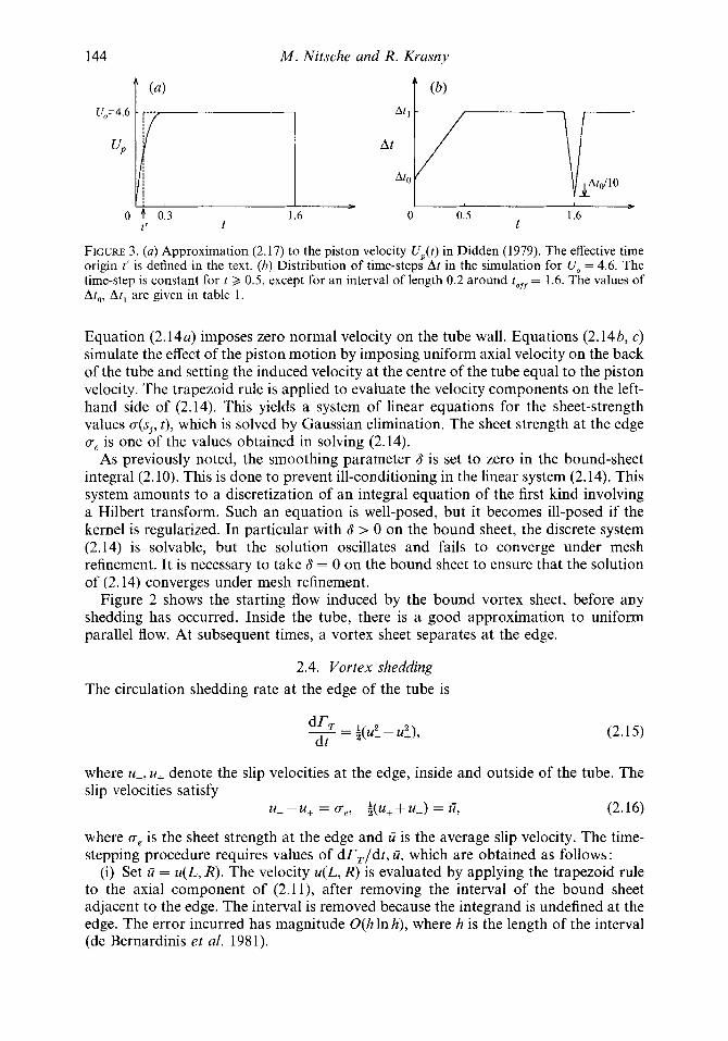
FIGURE 3. (a) Approximation (2.17) to the piston velocity U J t ) in Didden (1979). The effective time origin t' is defined in the text. (b) Distribution of time-steps At in the simulation for U, = 4.6. The time-step is constant for t 0.5, except for an interval of length 0.2 around t , = 1.6. The values of Ato, Atl are given in table 1.

Equation (2 .14~) imposes zero normal velocity on the tube wall. Equations (2.14h, c) simulate the effect of the piston motion by imposing uniform axial velocity on the back of the tube and setting the induced velocity at the centre of the tube equal to the piston velocity. The trapezoid rule is applied to evaluate the velocity components on the left- hand side of (2.14). This yields a system of linear equations for the sheet-strength values a(sj, t), which is solved by Gaussian elimination. The sheet strength at the edge re is one of the values obtained in solving (2.14).

As previously noted, the smoothing parameter 6 is set to zero in the bound-sheet integral (2.10). This is done to prevent ill-conditioning in the linear system (2.14). This system amounts to a discretization of an integral equation of the first kind involving a Hilbert transform. Such an equation is well-posed, but it becomes ill-posed if the kernel is regularized. In particular with 6 > 0 on the bound sheet, the discrete system (2.14) is solvable, but the solution oscillates and fails to converge under mesh refinement. It is necessary to take 6 = 0 on the bound sheet to ensure that the solution of (2.14) converges under mesh refinement.

Figure 2 shows the starting flow induced by the bound vortex sheet, before any shedding has occurred. Inside the tube, there is a good approximation to uniform parallel flow. At subsequent times, a vortex sheet separates at the edge.

2.4. Vortex shedding The circulation shedding rate at the edge of the tube is

= f(u? - u t ) , dT, dt

(2.15)

where t i c , u+ denote the slip velocities at the edge, inside and outside of the tube. The slip velocities satisfy

u--u+ = re, k(u++u-) = a, (2.16)

where re is the sheet strength at the edge and U is the average slip velocity. The time- stepping procedure requires values of dr,/dt, a, which are obtained as follows:

(i) Set U = u(L, R). The velocity u(L, R) is evaluated by applying the trapezoid rule to the axial component of (2.11), after removing the interval of the bound sheet adjacent to the edge. The interval is removed because the integrand is undefined at the edge. The error incurred has magnitude O(h In h), where h is the length of the interval (de Bernardinis et al. 1981).


(ii) Obtain the sheet strength ve by solving the linear system (2.14). (iii) From ve,a compute u+,u- using (2.16). Note that the shedding rate (2.15) is

insensitive to the sign of the slip velocity. However, a negative value of u+ or u- signifies attached slip flow on that side of the tube, while a positive value signifies separating flow. Hence, if either u+ < 0 or u- < 0, that value is set to zero to prevent an attached slip flow from contributing to the shedding process.

(iv) Using the values of u,, u-, obtain dr,/dt, fi from (2.15), (2.16). The continuous shedding process is simulated by releasing filaments from the edge

at regular time intervals. At the instant in which a new filament is released, it is convected with velocity (u, u) = (a, 0). This incorporates the normal boundary condition on the tube wall, u(L, R) = 0. The jth filament, shed at time t , is assigned circulation parameter value rj = rT(t).

2.5. Time-stepping and numerical parameters Equations (2.13), (2.15) form a coupled system of ordinary differential equations for the motion of the free filaments (xi, r i ) and the variation of the total shed circulation I',. The system is solved by the fourth-order Runge-Kutta method. Each time-step consists of four stages, a typical stage described as follows:

(i) Solve the linear system (2.14) for the bound-sheet strength values v(sj, t) . (ii) Evaluate the velocity (2.11) of the free filaments u(xi, rf), v(xi, r;). (iii) Evaluate the circulation shedding rate dr,/dt and average slip velocity a, from

(iv) Prepare for the next stage by updating (x:, rf), r,, U,(t). (2.15), (2.16), as described above.

After the fourth stage, the intermediate results are combined to obtain the values of (xi,.T>, I', at the new time level. Some details require further explanation. A new filament is shed only in the first stage of a time-step, not in the second to fourth stages. To prevent irregular point motion near t = 0, a numerical parameter r, controls the vortex shedding at small times. Until the condition rT 2 r, is satisfied, a newly shed filament is removed at the end of a time-step. Afterwards, each shed filament is retained in the computation, except after the piston stops moving, when every other filament is retained. Throughout the simulation, additional filaments are inserted on the free sheet whenever the distance between consecutive filaments is larger than e or when the angular separation (with respect to the spiral centre) is larger than 27c/N,.,,. Point insertion is performed using a piecewise cubic interpolating polynomial with the shedding time t as the interpolation parameter along the sheet. The elliptic integrals are computed using the method of arithmetic-geometric means (Bulirsch 1965).

The simulation is set up to closely match conditions in the experiment. The tube radius is R = 2.5 and the tube length is L = 10 (dimensional units of distance (cm), time (s) and velocity (cm s-l) are assumed throughout). Figure 3 (a) shows the driving velocity used in the simulation,

r

I O , t ' t0ff. The piston accelerates from rest to velocity U, during the interval 0 6 t 6 t,. The piston maintains constant velocity until t = tOff, when it stops moving. The numerical results refer mainly to the case U, = 4.6, t , = 0.3, tOff = 1.6 (as noted, some results


s N; N; At0 At1 r, E NVW

0.40 8 50 0.004 0.020 0.6 0.4 15 0.20 11 70 0.002 0.010 0.4 0.3 20 0.10 16 100 0.001 0.005 0.3 0.2 25

TABLE 1. Numerical parameters for driving velocity U, = 4.6. q, x: number of filaments on tube back and wall; At,, A t l : initial and final time-steps; r,: minimum initial shed circulation; E , N,,,: point insertion parameters controlling distance and angle between consecutive filaments.

refer to U, = 6.9, t, = 0.3, tOff = 1.1). The exponent 2.8 in (2.17) ensures that the piston stroke length

Lo = J"o.ff U,(t)dt

agrees with the experimental value (Lo = 7). Some plots will use the shifted time t , = t - t', where t' = 0.078 is the effective time origin defined by

[ Up(?) dt" = U,(t - t').

Figure 3(b) plots the distribution of time-steps used in the simulation. Small steps are required near t = 0, tOff owing to the variation in the driving velocity. Table 1 gives the numerical parameter values for the case U, = 4.6 (the values for U, = 6.9 are obtained by rescaling time). In practice, a value of the smoothing parameter 6 is chosen and then the remaining discretization parameters are refined until the computed solution is free of grid-scale features. It is apparent from table 1 that smaller values of 6 require greater numerical resolution.

3. Comparison between simulation and experiment 3. I Flow visualization

Figure 4(a) is the experimental flow visualization presented by Didden (1979) (see also van Dyke 1982, p. 43). The free shear layer appears as a streakline, marked by dye injected at the edge of the tube, in the vertical symmetry plane. The figure also shows the deformation of a material line which initially lies across the tube opening (the line has drifted slightly at t = 0 owing to residual fluid motion). The shear layer rolls up into a vortex ring, entraining the material line as it travels downstream. After the piston stops moving (toff = 1.6), a counter-rotating vortex ring forms at the edge of the tube. Figure 4(b) is the result of the simulation with smoothing parameter S = 0.2. The free vortex sheet is plotted along with a material line having the same initial shape as in the experiment. There is good agreement between simulation and experiment for the shape of the evolving shear layer and material line. This can be seen in more detail in figure 5, which presents an enlarged view of the experiment and simulation at t = 1.45. For t > tOff, the simulation captures the formation of the counter-rotating vortex ring. At the later times shown, the outer shape of the computed spiral has a similar degree of ellipticity to that in the experiment. A slight discrepancy occurs at t = 3.31 in that the gap between the two outer turns on the primary spiral is larger in the simulation than in the experiment. A possible explanation (N. Didden, private communication) is that swirl develops at late times in the experiment, causing the dye particles to leave the symmetry plane and narrowing the gap as viewed from the side.

Figure 6 shows the computed solution at t = 2.28 for three values of the smoothing


3.31 i FIGURE 4. Flow visualization of vortex-ring formation ( U , = 4.6, to, = 1.6). (a) Experiment, from

Didden (1979). (b) Simulation, S = 0.2.

parameter, 6 = 0.4, 0.2, 0.1. As 6 is reduced, the spiral core is more tightly rolled up. However, the core location and the shape of the outer turns are only weakly dependent on 6. Reducing 6 by half causes roughly a tenfold increase in the C.P.U. time. The simulation with 6 = 0.1 uses 2500 free filaments and requires 6 hours of C.P.U. time on a Sparc-10 workstation.


(b) 5.1 I

-5.1 8.0 1 0

FIGURE 5. Comparison at t = 1.45. (a) Experiment, from Didden (1979). (b) Simulation, S = 0.2.

3.2. Flow field Figure 7 shows the computed velocity field for 6 = 0.2, before and after the piston shutoff time. The vortex sheet and material line appear as a dashed curve in the lower half-plane. At t = tiff, the ring has moved away from the edge and the velocity across the tube exit-plane resembles a slug-flow profile. A small region of negative radial velocity occurs near the edge, arising from the ring-induced circulatory flow. As a result, the vortex sheet appears to leave the edge at a slight inward angle. A similar feature can be seen in the experiment (figure 5a). At t = t&, the velocity field near the edge is completely changed. The vortex ring induces a starting flow around the edge from outside to inside the tube, leading to the formation of a counter-rotating ring for t ’ t o w

Figure 8 presents the velocity profiles along the tube exit-plane for t < tOff . Didden’s (1979) experimental measurements are on the left and the computed profiles for 6 = 0.2 are on the right. As will be seen, the computed profiles are not uniformly valid up to the edge. In keeping with the idea of the vortex-sheet model as an asymptotic approximation for the outer flow, the computed profiles should be judged on the extent to which they capture the experimental flow away from the edge.

Figure 8(a, b) plots the axial velocity u(L, r ) for 0 < r < 2.5, across the tube opening. The experimental profiles satisfy the no-slip condition on the tube wall, but the computed profiles do not. Away from the wall however, there is reasonably good agreement between simulation and experiment. Owing to the starting flow around the edge, the axial velocity at small times has a peak near the wall. At later times, as the ring moves away from the edge, the axial velocity becomes almost uniform across the tube opening, increasing to a slightly higher value than the driving velocity U, = 4.6. At t = 1 .O, 1.6, the computed profile is uniform over a smaller portion of the opening than in the experiment.

Figure 8(c, d ) plots the axial velocity u(L, r ) for 2.5 < r < 3.5, outside the tube. At


0.5 L 4.5 4.5 r -

0.5 L 4.5

small times, again owing to the starting flow, the axial velocity is negative. The peak negative velocity increases in magnitude for t < 0.2, as the piston accelerates. The growing vortex ring displaces the starting flow away from the wall and induces positive axial velocity near the wall. This occurs earlier in the simulation than in the experiment. At later times, both the experimental and the computed axial velocity outside the tube approach a small positive value.

Figure 8(e,f> plots the radial velocity u(L, r ) for 1.4 < r < 3.3, across the edge. The radial velocity in the experiment falls to zero on both sides of the edge, but the computed velocity has a weak singularity at the edge owing to the jump in the smoothing parameter. At t = 0.1, the radial velocity is positive inside and outside of the tube, as expected for starting flow. For t 2 0.2, a region of negative radial velocity appears outside the tube owing to the developing ring-induced circulatory flow. At t = 1.0, 1.6, there is a good agreement between simulation and experiment for the radial velocity outside the tube. Inside the tube, the radial velocity in the experiment iKs positive, while the simulation predicts negative values at late times. Note that negative radial velocity inside the tube is consistent with the observation that the shear layer leaves the edge at a slight inward angle (figure 5) .

Didden (1979) noted that the boundary layer on the inner tube wall has a displacement effect, causing the flow to exceed the piston velocity U, = 4.6 as it exits the tube (figure 8a). A similar displacement and consequent speed-up occurs in the


(4 I . . . . . . . . . . . . . .

I . # . . . . . . . . . . . .

0 I _____ - - 7 - - ----- ----- ---c-

. . . . . . . . . . . . . . . . . . . . . . . . . . . . . . . . .

. . . . . . . . . . . . . . . . . . . . . . . . . . . . 10 15

FIGURE 7. Computed velocity field for S = 0.2. (a) t = tiIf, (b) t = tifT The free vortex sheet and material line appear as a dashed curve in the lower half-plane.

simulation (figure 8 b), arising there not from a boundary-layer effect but instead from the ring-induced negative radial velocity inside the tube (figure Sf). This alternative displacement mechanism may also play a role in the experiment.

Figure 9 plots the vorticity w(L, r ) for 2.1 < r < 3.4, across the edge. Didden (1979) obtained the vorticity by numerically differentiating the measured velocity. In the simulation, the vorticity is obtained by analytically differentiating the velocity (2.1 1). Since the bound sheet is not regularized, it induces irrotational flow away from the wall. Hence, the computed vorticity is associated entirely with the regularized free sheet. The prominent boundary layers in figure 9(a) are absent in figure 9(b), but simulation and experiment both predict a positive peak in vorticity outside the tube, away from the wall. As seen from the sketch in figure 9(a), taken from Didden (1979), this peak is associated with the ring vorticity. As the ring moves downstream away from the exit-plane, the peak amplitude decreases. The radial location of the peak moves outward, indicating that the ring diameter is increasing. At a given time, the peak vorticity in the simulation is significantly smaller than the experimentally measured value.

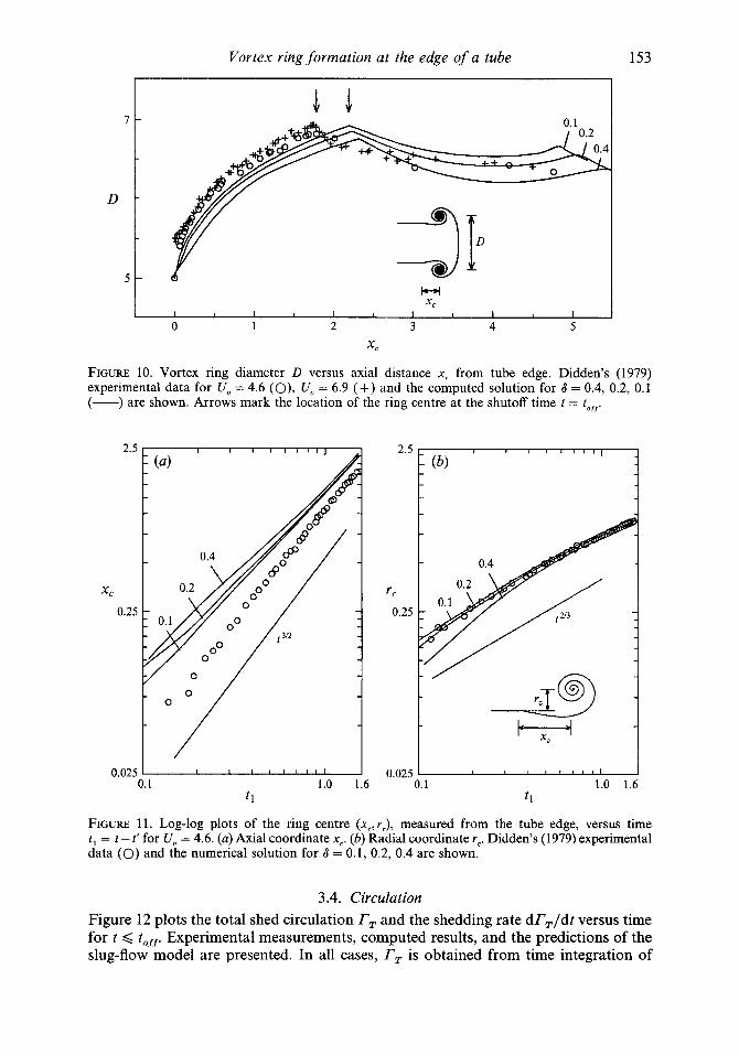
3.3. Vortex-ring trajectory Figure 10 plots the ring diameter D versus axial distance x, from the edge of the tube. In the simulation, the ring centre is taken to be the point of maximum vorticity. Experimental measurements for driving velocity U, = 4.6 (0) and U, = 6.9 (+) are shown, with computed results for smoothing parameter 6 = 0.4, 0.2, 0.1 (solid lines). The experimental results for U, = 4.6, t > toff were obtained from Didden's (1979) flow visualization. According to Didden (private communication), the difference in the ring trajectory for the two values of U, is probably due to a slight variation in the

Vortex ring-formation at the edge of a tube 151

6

5

4

3

2

1

U (cm s-I)

U (cm s

0 5 10 15 20 25

4

2

-9 0

-2

4

V (cm s-I)

3

2

1

0

-1

-2

26 28 30 32 34

5 - 1.6 ::g. I

4 - 0.3 0.4

3 - I

0. I i

0.6

0.2

I I u.l i

2l 1

0 0.5 1.0 1.5 2.0 2.5

(4 " I

L n x I

4 4 2.6 2.8 3.0 3.2 3.4

3 t 2

1

0

-1

-2

1.5 2.0 2.5 3.0 r

FIGURE 8. Velocity profiles along the tube exit plane at the indicated times (U, = 4.6). Didden's (1979) experimental data are given in (a, c , e). Computed results for S = 0.2 are given in (b , d,s). (a, b) Axial velocity u(L, r ) across tube opening, 0 < r < 2.5. (c , d ) Axial velocity u(L, r) outside the tube, 2.5 < r < 3.5. ( e , f ) Radial velocity v(L,r) across the edge, 1.4 < r < 3.3.

experimental procedure, rather than to a Reynolds-number effect. In the simulation, changing the driving velocity amounts to rescaling time and hence the computed trajectory is independent of U,.

The ring diameter increases for t < tOf f when the piston is moving, and decreases for t > tOf f after the piston is brought to rest. As 6 is reduced, the computed trajectory approaches the experimental measurements. Arrows indicate the location of the ring centre at the piston shutoff time. Note that the computed ring has travelled further than the experimental ring at t = tOf f . The diameter D does not decrease monotonically


w (s-

80

60

40

20

0

-20

4 0

4 0

-80

-100

-9

22 24 26 28 30 32

Y (mm)

-20 I

I I I I I

2.2 2.4 2.6 2.8 3.0 3.2 r

FIGURE 9. Vorticity along the tube exit-plane at the indicated times. (a) Experimental measurement (reproduced from Didden 1979). (b) Simulation (8 = 0.2).

for t > toff, but instead has a local maximum between x, = 4 and = 5. This feature could be caused by ‘tumbling’ in the core vorticity distribution. A similar feature has been observed in vortex-ring experiments by Weidman & Riley (1993).

Figure 11 presents log-log plots of the ring centre coordinates (x,, r,), measured from the edge of the tube, versus time t , = t - t’. Experimental measurements for U,, = 4.6 (0) are shown, with computed results for 6 = 0.4, 0.2, 0.1 (solid lines). The computed values of x, in figure 11 (a) lie above the experimental results by an amount which diminishes but does not vanish as S is reduced. This indicates that the computed ring has higher axial velocity than the experimental ring, consistent with the ring locations at t = toff in figure 10. The computed ring velocity was found to be 15-20% higher than values obtained from the experimental measurements. Figure 11 (b) shows good agreement between simulation and experiment for the radial coordinate I , . Didden (1979) found that for t , < 0.6, the ring coordinates increase approximately as x, - t;/2, I , - t:/3. This behaviour is also seen in the simulation. In $4, the observed ring trajectory will be compared with similarity theory for starting flow around an edge.


I

D

5

5 . c 0.1

H xc

I I I I I I

0 1 2 3 4 5

xc

FIGURE 10. Vortex ring diameter D versus axial distance x, from tube edge. Didden’s (1979) experimental data for U, = 4.6 (O), U,, = 6.9 (+) and the computed solution for S = 0.4, 0.2, 0.1 (-) are shown. Arrows mark the location of the ring centre at the shutoff time t = t o f f .

2.5

xc 0.25

0.025 I 1 I I I I I , , I I

0.1 1.0 1.6 tl

2.5

0.25

0.025 I I

0.1 1.0 1.6 tl

FIGURE 11. Log-log plots of the ring centre (xc, rc), measured from the tube edge, versus time t , = t - t’ for U, = 4.6. (a) Axial coordinate x,. (b) Radial coordinate rc. Didden’s (1979) experimental data (0) and the numerical solution for S = 0.1, 0.2, 0.4 are shown.

3.4. Circulation Figure 12 plots the total shed circulation rT and the shedding rate drT/dt versus time for t < tofr Experimental measurements, computed results, and the predictions of the slug-flow model are presented. In all cases, r, is obtained from time integration of


I I L I I I I -10 0 0.4 0.8 1.2 1.6 0 0.4 0.8 1.2 1.6

t t

l/.'O.l 0.2 0.4

-20 - 0 0.4 0.8 1.2 1.6

t

FIGURE 12. (a) Total shed circulation r,. (b) Circulation r,, r, shed from inner, outer tube edges respectively. (c) Circulation shedding rate dr,/dt, dFJdt. Didden (1979) (-----), simulation (-), slug flow (. . . . . .). Computed results for S = 0.4, 0.2, 0.1 are shown.

dr,/dt. Didden (1979, 1982) obtained the shedding rate from the velocity and vorticity profiles in the exit-plane,

= lor+ w(L, r ) u(L, r ) dr, dt

where r+ is the edge of the boundary layer outside the tube. In the simulation, the shedding rate is given in terms of the slip velocities at the edge, dr,/dt = f(u: - ut) . In the slug-flow model, the shedding rate is determined by the piston velocity, dr,/dt = $Up.

Figure 12(a) shows that the simulation overestimates the total shed circulation r,. The computed values of r, decrease as 6 is reduced, but they remain bounded away from the experimentally measured values. The higher total circulation in the simulation explains the higher axial velocity of the computed ring (figure 11a). The slug-flow model underestimates the total shed circulation.


Figure 12(b) plots ri,ro, the circulation shed from the inner and outer tube walls, versus time. Didden (1979) obtained the shedding rates dri/dt, dI',/dt as in (3.2), with appropriate limits of integration. In the simulation dr t /dt = :u2 and dr,/dt = -fu;, while in the slug-flow model, dr,/dt = dr,/dt and dr,/dt = 0. The inner circulation Ti is higher in the simulation than in the experiment, but the discrepancy is less than in T, (figure 12a). The situation is reversed for the outer circulation, the computed values of T, having smaller magnitude than the experimental measurements. For the slug-flow model, the discrepancy with experiment is increased over figure 12(a).

Figure 12(c) plots the inner and outer shedding rates dr,/dt, dI',,/dt versus time. In the experiment, the inner rate increases for t < 0.3 as the piston accelerates, and then decreases slowly to a positive steady-state value as the piston moves with constant velocity. In the simulation dr,/dt has a sharp initial peak which decreases as S is reduced, but still remains significantly higher than the experimental peak. Over longer times, the computed value of dri/dt approaches the experimental steady-state value as 6 is reduced. By comparison, the slug-flow model underestimates the inner steady-state shedding rate. The outer shedding rate dro/dt has a peak in both simulation and experiment near t = 0.3, when the edge of the ring is crossing the exit-plane. The peak value of dr,/dt is smaller in the simulation than in the experiment. For t > 0.3, the outer shedding rate approaches zero although this occurs more rapidly in the simulation.

The main error in the computed circulation occurs at small times, when the simulation over-estimates the inner shedding rate dr,/dt. This leads to higher computed values of total circulation I', and consequently higher axial velocity for the computed ring. The error in dri/dt at small times is attributed mainly to the neglect of detailed viscous effects in the vortex-sheet model although discretization and smoothing errors may be partly responsible. At late times prior to piston shutoff, the inner and outer shedding rates in the simulation approach steady-state values in good agreement with experiment.

4. The relation between similarity theory and observation In the similarity theory for starting flow past a sharp edge, the fluid motion takes

place in the complex z-plane with the negative x-axis considered as a semi-infinite flat plate. At t = 0, the complex potential has the form @ = czl/', corresponding to singular flow around the edge (figure 13a). For t > 0, a vortex sheet separates at the edge and rolls up into a spiral in a self-similar manner. It follows from dimensional analysis that the coordinates of the spiral centre obey the power laws, x, - PI3, y , - PI3.

Pullin (1978) computed the self-similar shape of the vortex sheet and found that x, < 0, y , > 0. Hence, similarity theory predicts that the starting vortex follows a straight-line trajectory, travelling upstream above the plate.

It is plausible to assume that this theory applies to the axisymmetric problem during an initial time interval in which the core size of the vortex ring is small compared with the tube diameter. Using this approach, Saffman (1978) and Pullin (1979) have analysed the ring formation process. However, as previously noted, there is a discrepancy between similarity theory and the ring trajectory observed in experiment and simulation. In particular, the observed ring coordinates behave approximately as x, - t;/', r, N t;13, with x,, r, > 0, so that the ring follows a curved trajectory, travelling downstream away from the edge.

Didden (1979) attributed the discrepancy to the theory's neglect of the self-induced ring velocity. Subsequently, Auerbach (1987 a, b) performed an experimental study of

156

(4

M . Nitsche and R. Krasny

(b)

FIGURE 13. Starting flow at an edge. (a) Flat plate (similarity theory). (6) Circular tube (simulation).

two-dimensional vortex-pair formation at the edge of a rectangular tube. He observed the same behaviour in the trajectory of the rectilinear pair as is seen in the axisymmetric ring. From this he concluded that in the case of the vortex-ring, axisymmetry is not responsible for the discrepancy between theory and observation. He also discounted the effects of distant boundary geometry, viscous diffusion, and shear-layer thickness. Searching for a common factor to explain both the axisymmetric and the rectilinear cases, Auerbach (1987a) concluded that the discrepancy is caused by the theory’s neglect of either secondary vorticity generated on the outer tube wall or viscous entrainment by the developing jet. The following discussion seeks to clarify the role of these various factors, using insight gained from the simulation.

Self-induced velocity. The axisymmetric ring has self-induced velocity in the downstream direction owing to the curvature of its filaments. The rectilinear vortex pair studied in Auerbach (19874 has an analogous self-induced velocity because each line filament in the pair has a counter-rotating image across the tube centreline. This is true whether the experiment is performed with two salient edges or with one edge and a bounding plate on the tube centreline (in the latter case, the image filament is bound in the plate). These factors, filament curvature in the axisymmetric case and image vorticity in the rectilinear case, are absent in the similarity theory. As a result, the starting vortex in the similarity theory has no self-induced downstream velocity.

StartingJlow. Figure 13 (b) shows the starting flow in the simulation, near the edge of the circular tube. The axisymmetric starting flow contains a singular component around the edge similar to figure 13(a). However, an additional downstream component is present in figure 13(b). To clarify this, note that the complex potential for a general two-dimensional starting flow has the form Q, = c1 z1’2 + c2 z+ . . . (Auerbach 1987a; Graham 1983). The first term is the singular starting flow of similarity theory (figure 13 a). The second term is an additional component representing uniform flow parallel to the edge. In the rectilinear case, bound vorticity on one edge induces such an additional component in the starting flow at the other edge. In the axisymmetric case, a similar effect arises from the curvature of the bound filaments on the tube. In either case, for both the axisymmetric ring and the rectilinear pair, the starting flow contains a downstream component which is absent in the similarity theory. In both cases, the geometry of the solid boundary is responsible for the discrepancy with similarity theory.


Secondary vorticity. For t < tOff, primary vorticity (positive) is shed from the inner tube wall and secondary vorticity (negative) is shed from the outer wall. Auerbach (1987 a) asserted that similarity theory fails to incorporate secondary vorticity and he proposed this as an explanation for the discrepancy between theory and observation. However, similarity theory uses the same shedding rate (2.15) on which the simulation is based. Hence the theory does take into account secondary vorticity, by altering the circulation shedding rate in response to the slip velocity outside the tube. Admittedly, some important aspects of secondary separation are not captured by similarity theory, especially for flow past a wedge (Pullin & Perry 1980). Moreover, the simulation underestimates the experimentally measured shedding rate outside the tube (figure 12c). Still, the agreement between simulation and experiment, for the observed ring trajectory, suggests that secondary vorticity is not responsible for the discrepancy between theory and observation.

Viscous diflusion, viscous entrainment, shear-layer thickness. These factors are neglected in both the similarity theory and the simulation (the smoothing parameter may represent thickness in a crude way, but presumably not in a detailed sense). In view of the agreement seen between simulation and experiment, these factors apparently do not play a significant role in determining the ring trajectory in the present problem.

Driving velocity. For a precise comparison with similarity theory, the piston should accelerate instantaneously from rest to velocity U,. However, in both experiment and simulation, the piston attains velocity U, over a finite time interval. The absence of a genuine impulsive start in the piston velocity may contribute to the discrepancy between theory and observation.

Didden (1982) noted that similarity theory also fails to predict the observed linear increase T, N t in total shed circulation (figure 12). He pointed out that while the slug- flow model predicts this feature, it underestimates the inner shedding rate (figure 12c). He attributed the underestimation of dT'Jdt to the absence of the boundary-layer displacement effect in the slug-flow model. As already noted, displacement occurs in the simulation due to the ring-induced circulatory flow (figure 7, 8b). The relative importance of the two displacement mechanisms is presently not known.

Before leaving this section, it should be emphasized that the ring trajectory and circulation shedding rate have not been extensively investigated at small times. The singular component of the starting flow should be dominant in such a regime. For this reason, as well as the absence of a genuine impulsive start, the present results do not rule out the possibility that similarity theory does describe axisymmetric vortex sheet roll-up at small times. This issue is left for future investigation.

5. Conclusions An axisymmetric vortex-sheet model has been applied to simulate Didden's (1979)

experiment on vortex-ring formation. The computed results were compared with the experimental measurements. The findings are summarized below.

(i) There is good agreement between simulation and experiment for the flow visualization of the ring formation process. The simulation correctly predicts the ring trajectory, although the computed ring travels N 15-20 % faster than the experimental ring.

(ii) The ring is observed to travel downstream in experiment and simulation, while similarity theory predicts that it travels upstream. The discrepancy is attributed to three factors: the theory's neglect of the self-induced ring velocity (Didden 1979), the

6 F L M 216


absence of a downstream component in the theory's starting flow, and the absence of a genuine impulsive start in experiment and simulation.

(iii) The ring coordinates increase approximately as x, - t3I2, r , - t2I3 in experiment and simulation, while similarity theory predicts the exponent 2/3 for both coordinates. The agreement in the radial exponent may be coincidental in view of the theory's failure to predict the axial exponent. There is currently no theoretical explanation for the apparent power-law increase of the ring coordinatest.

(iv) At small times, the computed values of the inner shedding rate exceed the experimental measurements. This leads to higher circulation in the computed ring and is responsible for the higher axial velocity of the computed ring. At late times prior to piston shutoff, the computed circulation shedding rates agree well with experiment. The discrepancy in the initial circulation shedding rate is attributed to the neglect of detailed viscous effects in the vortex sheet model.

(v) The outer shape of the computed ring is fairly insensitive to the value of the smoothing parameter used in the simulation. There is generally improved agreement between simulation and experiment as the smoothing parameter is reduced.

This work drew inspiration from the experimental study performed by Dr Norbert Didden. We are grateful to him for permission to reproduce figures from his published work. R. K. wishes to thank Dr Karim Shariff for a stimulating discussion which was the catalyst for this work. The results are based on the PhD thesis of Nitsche (1992). We thank one of the referees for suggesting the example discussed in the Appendix. The work was supported by NSF grant DMS-9204271. R.K. is grateful to the UCLA Mathematics Department and Professor Russel Caflisch for hospitality and support provided through NSF grant DMS-9306720 on a sabbatical visit, during the preparation of the final manuscript. The computations were performed at the University of Michigan and the NSF San Diego Supercomputer Center.

Appendix. Evaluation of the induced velocity at the edge Consider a flat two-dimensional vortex sheet of uniform strength located on the

interval y = 0, -L < x < L. The left and right halves of the interval represent the bound and free sheets in the simulation. The origin (x, y ) = (0,O) corresponds to the edge of the tube in the simulation. The smoothing parameter 6 is zero for x < 0 and non-zero for x > 0, and the interval ( - e , 0) on the bound sheet is removed. The following discussion analyses the error in evaluating the induced velocity at the origin. The two components of velocity behave differently and they are discussed separately.

Tangential cornponen t

The exact value of the tangential velocity at a general point (x ,y) is

t (Added in proof) The experimental data do not exhibit power law behaviour x, - ta, Y, - tp over the entire interval 0 < t < tOfr Didden (1979) suggested the values a = 3/2, /l = 2/3 for t < 0.6, but the coordinates grow less rapidly at later times (see his figure 6, present figure 11 a). K. Shariff (private communication) noted that the x, data could be fit about equally well by a = 4/3, and proposed a theoretical justification for this value based on the self-similar growth of circulation, r - PI3, and the relation dx,/dt - T / R . M. Gharib (private communication) pointed out that in the simulation with S = 0.1, x, obeys a power law up to t = t O f f , with a = 1.2 (figure 11 a). This is closer to the value a = 1 obtained in recent experiments by Weigand & Gharib (1994).


This component has a jump discontinuity across the sheet,

u, = lim u(0,y) = -:, u- = lim u(0,y) = i. (A 2) y+n+ y+n-

The tangential velocity on the sheet itself is defined to be the average of the one-sided limits,

The approximation to the tangential velocity is

u(0,O) = i(u+ + u-) = 0. (A 3)

X + tan-1( 0 2 + n1/2)]}. (A4)

The approximation is continuous across the sheet,

and it agrees with the exact value given by (A 3). In the simulation, the tangential velocity at the edge is evaluated by applying the

trapezoid rule to the axisymmetric analogue of the induced velocity integral (A 4). The reason for removing the interval (- E , 0) is that the first integrand on the right of (A 4) is undefined for (x, y ) = (0, 0), s = 0. As shown by (A 5), removing the interval incurs zero error in the two-dimensional case. In the axisymmetric case, the error has size O(slnc), a result which follows from analysis similar to that given by de Bernardinis et al. (1981).

Normal component The exact value of the normal velocity is

(x-s)ds 1 (L+x)'+y2 - _ - 4 X , Y ) = - (x - $2 +y2 4n log (L - x)2 +y2 *

This component is continuous across the sheet (the singularities at x = f L are irrelevant for this discussion). At the origin, the exact value is

v(0,O) = 0. (A 7) The approximate value of the normal velocity is

At the origin, this gives

The approximate value is incorrect in the limit 6-t 0, unless E = 6. In the simulation 6-2


however, the normal velocity at the edge of the tube is not obtained by evaluating the induced velocity integral. Instead, the value is set to zero, by application of the boundary condition on the tube wall.

Remarks (i) If (x , y ) lies away from the bound sheet, then

lim %,€(&Y) = &,Y), lim %,E(X,Y) = 4 G Y ) . (A 10) (6, + 4 o , 0 ) (6 , h)'(O, 0 )

In other words, the approximation converges to the correct result in this case regardless of how the limit (6, e)+ (0,O) is taken. In practice, the simulation sets e = 0 when computing the induced velocity at a free vortex filament.

(ii) The approximate tangential velocity u6, J x , y ) is uniformly bounded, but the normal velocity U ~ , ~ ( X , y ) diverges as (x, y ) + (0,O) for e = 0, 6 > 0. This is reflected by cusps at Y = 2.5 in the velocity profiles of figure S d f ) (although quadrature error on the bound sheet prevents an actual divergence from occurring). In the simulation, the free filaments are advected away from the edge and the divergence of the normal velocity at the edge has not caused difficulty. This implies that while the approximate velocity is not uniformly valid up to the edge, it appears to be valid away from the edge.

R E F E R E N C E S

ACTON, E. 1980 A modelling of large eddies in an axisymmetric jet. J. Fluid Mech. 98, 1 . ANDERSON, C. 1985 A vortex method for flows with slight density variations. J . Comput. Phys. 61,

417. AUERBACH, D. 1987a Experiments on the trajectory and circulation of the starting vortex. J. Fluid

Mech. 183, 185. AUERBACH, D. 19876 Some three-dimensional effects during vortex generation at a straight edge.

Exp. Fluids 5 , 385. BERNARDINIS, B. DE, GRAHAM, J. M. R. & PARKER, K. H. 1981 Oscillatory flow around disks and

through orifices. J. Fluid Mech. 102, 279. BULIRSCH, R. 1965 Numerical calculation of elliptic integrals and elliptic functions. Numer. Maths

7 , 78. CAFLISCH, R. & LI, X. 1992 Lagrangian theory for 3D vortex sheets with axial or helical symmetry.

Trans. Theory Statist Phys. 21, 559. CAFLISCH, R., LI, X. & SHELLEY, M. 1993 The collapse of an axi-symmetric, swirling rotex sheet.

Nonlinearity 6, 843. CHORIN, A. J. & BERNARD, P. S . 1973 Discretization of a vortex sheet, with an example of roll-up.

J . Comput. Phys. 13, 423. CLEMENTS, R. R. & MAULL, D. J. 1975 The representation of sheets of vorticity by discrete vortices.

Prog. Aero. Sci. 16, 129. DAHM, W. J. A., FRIELER, C. E. & TRYGGVASON, G. 1992 Vortex structure and dynamics in the near

field of a coaxial jet. J . Fluid Mech. 241, 371. DAVIES, P.O.A.L. & HARDIN, J. C. 1974 Potential flow modelling of unsteady flow. In Numerical

Methods in Dynamics (ed. C. A. Brebbia & J. J. Connor), p. 42. Pentech. DIDDEN, N. 1979 On the formation of vortex rings: rolling-up and production of circulation. 2.

Angew. Math. Phys. 30, 101. DIDDEN, N. 1982 On vortex formation and interaction with solid boundaries. In Vortex Motion (ed.

E.-A. Muller), p, 1 . Vieweg & Sohn. GRAHAM, J. M. R. 1983 The lift on an aerofoil in starting flow. J . Fluid Mech. 133, 413. GRAHAM, J. M. R. 1985 Application of discrete vortex methods to the computation of separated

flows. In Numerical Methods for Fluid Dynamics II, (ed. K. W. Morton & M. J . Baines), p. 273. Clarendon.


KANEDA, Y . 1990 A representation of the motion of a vortex sheet in a three-dimensional flow. Phys.

KRASNY, R. 1986 Desingularization of periodic vortex sheet roll-up. J . Comput. Phys. 65, 292. KRASNY, R. 1991 Vortex sheet computations : roll-up, wakes, separation. Lectures in Applied

LAMB, H. 193 1 Hydrodynamics. Cambridge University Press. LEONARD, A. 1980 Vortex methods for flow simulation. J. Comput. Phys. 37, 289. MARTIN, J. E. & MEIBURG, E. 1991 Numerical investigation of three-dimensionally evolving jets

subject to axisymmetric and azimuthal perturbations. J. Fluid Mech. 230, 271. NITSCHE, M. 1992 Axisymmetric vortex sheet roll-up. PhD thesis, University of Michigan. PRANDTL, L. 1927 The generation of vortices in fluids of small viscosity. J . R. Aero. SOC. 31, 718. PUGH, D. A. 1989 Development of vortex sheets in Boussinesq flows - formation of singularities.

PULLIN, D. I . 1978 The large-scale structure of unsteady self-similar rolled-up vortex sheets. J . Fluid

PULLIN, D. I. 1979 Vortex ring formation at tube and orifice openings. Phys. Fluids 22, 401. PULLIN, D. I. & PERRY, A. E. 1980 Some flow visualization experiments on the starting vortex.

SAFFMAN, P. G. 1978 The number of waves on unstable vortex rings. J. Fluid Mech. 84, 625. SARPKAYA, T. 1989 Computational methods with vortices - the 1988 Freeman Scholar Lecture.

SHARIFF, K. & LEONARD, A. 1992 Vortex rings. Ann. Rev. Fluid Mech. 24, 235. TRYGGVASON, G., DAHM, W. J. A. & SBEIH, K. 1991 Fine structure of vortex sheet roll-up by viscous

VAN DYKE, M. 1982 An Album of Fluid Motion. Parabolic Press. WEIDMAN, P. D. & RILEY, N. 1993 Vortex ring pairs: numerical simulation and experiment. J. Fluid

Mech. 257, 31 1-337. WEIGAND, A. & GHARIB, M. 1994 On the evolution of laminar vortex rings. Preprint.

Fluids A 2, 458.

Mathematics, vol. 28, p. 385. AMS.

PhD thesis, Imperial College, London.

Mech. 104, 45.

J . Fluid Mech. 97, 239.

Trans ASME I : Fluids Engng 1 11, 5.

and inviscid simulation. Trans. ASME I : J. Fluids Engng 113, 31.

a numerical study of vortex ring formation at the edge of a

Documents