A Numerical Study of ‘‘Hijikawa-Arashi’’: A Thermally Driven GapWind Visualized by Nocturnal Fog

JUNSHI ITO

Atmosphere and Ocean Research Institute, The University of Tokyo, Kashiwa, Chiba, Japan

TOSHIYUKI NAGOSHI

Iwate University, Morioka, Iwate, Japan

HIROSHI NIINO

Atmosphere and Ocean Research Institute, The University of Tokyo, Kashiwa, Chiba, Japan

(Manuscript received 20 July 2018, in final form 15 March 2019)

ABSTRACT

A renowned local wind in Japan, ‘‘Hijikawa-Arashi,’’ is a thermally driven nocturnal gap wind ac-

companied by fog. The wind is visually identified by the fog along the valley of the Hijikawa River between

the Ozu basin and the Seto Inland Sea during the early morning in autumn and winter. A fine-resolution

numerical model is employed to reproduce the main observed features of Hijikawa-Arashi. A vertical

resolution of 10 m or less at the lowest level is required to express the nocturnal radiative cooling of the

land that is required for fog formation in the basin, and fine horizontal resolution is necessary to express a

realistic valley through which the fog is advected to the sea. Multiple hydraulic jumps accompanied by

supercritical flow occur because of the complex topography. Both moisture transport by the sea breeze

during the daytime and evaporation from the land surface are important for accumulating moisture to

produce the fog.

1. Introduction

‘‘Hijikawa-Arashi’’ is the Japanese name for a stormy

wind that blows along the Hijikawa River in Ozu City,

Ehime Prefecture, Shikoku Island, Japan (Fig. 1). It is

a southeasterly wind that blows from the Ozu basin to

the estuary of the Hijikawa River. A unique feature of

Hijikawa-Arashi is that it can be observed without in-

struments because it is fascinatingly visible because of

the accompanying radiative fog that develops from the

surface in the Ozu basin during a clear night with calm

winds (Fig. 2; see supplemental movie S1 in the online

supplemental material and the description therein). It oc-

curs in early morning during late autumn and early winter

when the synoptic pressure gradient is weak and the

weather is fair, and is most frequent in November. The

magnificent scenery of Hijikawa-Arashi is one of the nat-

ural tourist attractions in that region, and the local gov-

ernment, Ozu City, maintains a panoramic viewpoint in a

park on a hill adjacent to the Hijikawa River (point 2 in

Fig. 3a; Fig. 3b).

The topography around the region where Hijikawa-

Arashi occurs is quite complex. The Hijikawa River has a

number of branches that originate from the westernmost

edge of the mountain range on Shikoku Island (Fig. 1c).

Many of these branches first flow southward, which is op-

posite to the final flow direction of theHijikawa to the Seto

Inland Sea in the north.1 These branches join together in

Denotes content that is immediately available upon publica-

tion as open access.

Supplemental information related to this paper is available at the

Journals Online website: https://doi.org/10.1175/JAMC-D-18-0189.s1.

Corresponding author: Junshi Ito, junshi@aori.u-tokyo.ac.jp

1 In fact, ‘‘Hiji’’ in Japanese means an arm representing an arm

bent at the elbow and ‘‘Kawa’’ means river, so that ‘‘Hijikawa’’

means a river with a large bend.

JUNE 2019 I TO ET AL . 1293

DOI: 10.1175/JAMC-D-18-0189.1

� 2019 American Meteorological Society. For information regarding reuse of this content and general copyright information, consult the AMS CopyrightPolicy (www.ametsoc.org/PUBSReuseLicenses).

Unauthenticated | Downloaded 01/11/22 08:37 AM UTC

the Ozu basin to form a single final channel of 10-km

length, where the river flows out to the Seto Inland Sea

through a narrow valley. At its narrowest, the valley is

about 100mwide (Fig. 1c), and the elevation of the valley

bottom within the basin is only ;10m above sea level.

The dynamics of Hijikawa-Arashi do not appear to be

the same as those of many other local winds reported

in the literature, as discussed by Ohashi et al. (2015).

Hijikawa-Arashi may be classified as a type of gap wind,

which is defined as a strong low-level wind through a

channel or a gap driven by a pressure gradient (see

http://glossary.ametsoc.org/wiki/Gap_wind). Mayr et al.

(2007) presented a comprehensive review of the dy-

namics of gap wind, and Ohashi et al. (2015) presented a

list of studies of gap winds.

Most gap winds are driven by a pressure gradient that

is imposed by a synoptic-scale disturbance. However, in

some cases, gap winds are driven by the diurnal thermal

contrast between a large plain and a smaller basin or

valley that has a lesser heat capacity. These gap winds

are likely to reverse their direction during the daytime

and nighttime transitions (e.g., Zängl 2004; Chrust et al.2013; Finn et al. 2016). For gaps with larger scales, on the

other hand, both of the synoptic pressure gradient and

thermal contrast can play important roles (e.g., Liu et al.

2000; Banta et al. 2004;Wagenbrenner et al. 2018). Chrust

et al. (2013) reported a strong local nocturnal wind at the

exit of a narrow canyon, Weber Canyon (Utah), in the

United States. They called this wind a ‘‘thermally driven

valley-exit jet’’ to distinguish it from the ordinary gap

winds driven by a synoptic pressure gradient.

Hijikawa-Arashi appears to be similar to the wind

reported by Chrust et al. (2013), yet differs with respect

to the following points. 1) As mentioned above, there is

only aweak slope of the valley bottom along theHijikawa

River, so that katabatic downslope acceleration (as is

important for nocturnal valley winds; e.g., Whiteman

1990) is negligible. 2) The horizontal thermal contrast

across the valley along the Hijikawa River is mainly

between the air over the Seto Inland Sea and that in the

Ozu basin. This contrast is larger than that between the

sea and the coastal area or between the coastal area

FIG. 1. Topographic maps of (a) Japan, (b) Shikoku Island, and (c) theOzu basin. The red square in (a) indicates the area shown in (b), and

the red rectangle in (b) indicates the area shown in (c). Blue lines in (c) indicate the Hijikawa River and its major branches.

FIG. 2. Airborne photograph of Hijikawa-Arashi. Viewed from the Seto Inland Sea in the (a) northeast and

(b) north of the Nagahama estuary on 5 Nov 2014 (courtesy of Ozu City).

1294 JOURNAL OF APPL IED METEOROLOGY AND CL IMATOLOGY VOLUME 58

Unauthenticated | Downloaded 01/11/22 08:37 AM UTC

and the basin. 3) The fog may contribute to nocturnal

cooling in the Ozu basin, and it might affect the char-

acteristics of the wind in addition to visualizing the

wind. 4) As will be shown in the discussion, enhance-

ment of the wind speed of Hijikawa-Arashi is signifi-

cant not only at the valley exit (estuary), but also at the

right downstream of a gap in the middle of the valley.

Therefore, we will call Hijikawa-Arashi a ‘‘thermally

driven gap wind.’’

Ohashi et al. (2015) carried out surface observations

along the Hijikawa River and investigated the environ-

mental conditions that favor the occurrence of strong

wind at the estuary, whereas Ohashi et al. (2018) con-

ducted observations to investigate thermo-physiological

impacts of the cold winds on people. Several other

studies of Hijikawa-Arashi have been published in

Japanese. For example, Nagoshi (2009) studied the

wind in a laboratory experiment using a scale model

of the topography of the valley. Numerical studies on

Hijikawa-Arashi have been also conducted, using the

Cloud Resolving Storm Simulator (CReSS; Tsuboki and

Sakakibara 2002) with a horizontal resolution of 300m,

and Nagoshi et al. (2013) successfully reproduced fog

in the Ozu basin and the strong local wind at the estuary

for the observed case of 5 January 2010. However, the

horizontal resolution of their study was not fine enough

to resolve the narrowest part of the valley. These

authors attempted to further improve the horizontal

resolution, but a numerical instability prevented their

calculation. Shigeta (2009) used theWeatherResearch and

Forecasting (WRF) Model to reproduce the intensified

near-surface wind at the estuary and discussed its ver-

tical profile.

To reproduce a realistic Hijikawa-Arashi, a numerical

model with full physics is required, which includes re-

alistic topography, fog generation, and radiation. In

particular, the model needs to employ very fine resolu-

tion to resolve the narrow valley along the Hijikawa

River, although a relatively small calculation domain

may be used since Hijikawa-Arashi occurs under a weak

pressure gradient in a moving high.

The present study undertook a numerical simula-

tion of two cases of Hijikawa Arashi using a JMA

nonhydrostatic model (Saito et al. 2006). The aim is to

reproduce not only the strong wind speed of Hijikawa-

Arashi but also the way in which it is visualized by fog

and to understand its dynamics. Very high horizontal

resolution of 80m and fine vertical resolution of 5m

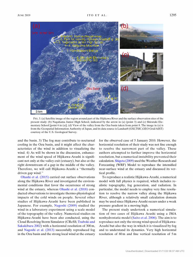
FIG. 3. (a) Satellite image of the region around part of the HijikawaRiver and the surface observation sites of the

present study: (b) Nagahama Junior High School, indicated by the arrow in (a) (point 3) and (c) Shirataki Ele-

mentary School [point 6 in (a)]. (d) View of the valley from the Ozu basin taken from point 8. The image in (a) is

from the Geospatial Information Authority of Japan, and its data source is Landsat8 (GSI,TSIC,GEOGrid/AIST)

courtesy of the U.S. Geological Survey.

JUNE 2019 I TO ET AL . 1295

Unauthenticated | Downloaded 01/11/22 08:37 AM UTC

near the surface were used to realistically reproduce

the phenomena.

The remainder of this paper is organized as follows.

Section 2 describes the numerical model and its configu-

ration, the two cases to be simulated, and the surface ob-

servations used to verify the simulation results. Section 3

gives an overview of the numerical results at various res-

olutions, and section 4 compares the numerical results with

surface observations. Section 5 discusses resolution de-

pendence, dynamics, and the processes that accumulate

moisture to form the fog. Finally, concluding remarks are

presented in section 6.

2. Experimental design and target cases

a. Numerical model

Thepresent studyuses the JapanMeteorologicalAgency’s

Non-HydrostaticModel (JMA-NHM),which is one of the

regional NWP models used for operational forecasts by

the JMA (Saito et al. 2006). Like other NWPmodels, this

model considers many physical processes that are rele-

vant to the atmosphere, surface–atmosphere interaction,

and soil. The present study employs the Deardorff (1980)

turbulence scheme, the Beljaars and Holtslag (1991)

surface-layer parameterization, bulk cloud microphysics,

and long- and shortwave radiation. Three kinds of ex-

periments were carried out by changing the resolution as

follows:

1) Experiment CC with coarse vertical and horizontal

resolution,

2) Experiment FC with fine vertical and coarse hori-

zontal resolution, and

3) Experiment FF with fine vertical and horizontal

resolution.

The configuration of each experiment is listed in Table 1.

There were 3 times as many vertical levels for Experi-

ments FC andFF as for Experiment CC, while themodel

top height for Experiments FC and FF was lower than

for Experiment CC. Thus, the vertical resolution of

the lower layers in Experiments FC and FF was about

4 times as fine as that in Experiment CC.

Initial and boundary conditions of Experiments CC

and FC were given by interpolating the Meso Analysis

(MANL)2 provided by the JMA, whereas those of Ex-

periment FFwere given by the output of Experiment FC

every 5min. Sea surface temperatures (SSTs) are also

given by interpolating the dataset for each day provided

by JMA, but their changes are very small.

The computational domain and topography for each

experiment are shown in Fig. 4. Terrain-following coor-

dinates (Saito et al. 2006) were used, and the topography

and land were generated by smoothing the 50-m mesh

map provided by the Geospatial Information Authority

of Japan. The maximum gradient of topography in the

numerical model was suppressed to 0.5. The valley along

theHijikawaRiver is so narrow that experimentswith the

coarser horizontal resolution (Experiments CC and FC)

cannot resolve it adequately, and artificial saddles

appear in the valley (Fig. 5a). On the other hand, the

experiment with the finer horizontal resolution (Ex-

periment FF) is sufficient to resolve the river path even

at the narrowest part of the valley. Some grid cells at the

river were assigned as water surface in Experiment FF,

although the river is imperfectly resolved and thus is

discontinuous (Fig. 5b).

b. Case overview and field observations

The present study investigates two case studies of ob-

served Hijikawa-Arashi: one on 4 January 2015 that is

referred to as Case J and the other on 4 November 2015

(Case N; supplemental movie S1). In both cases, the area

was covered by synoptic highs, and fine weather is

generally expected (Fig. 6). According to data of sur-

face observatories operated by the JMA, the nighttime

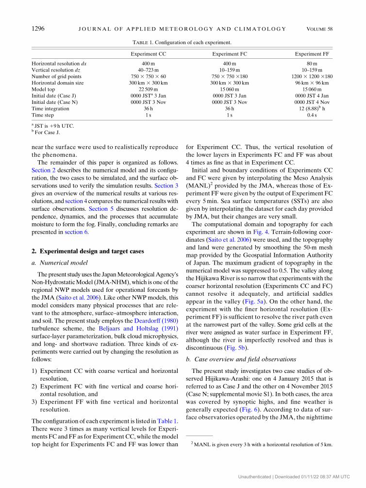
TABLE 1. Configuration of each experiment.

Experiment CC Experiment FC Experiment FF

Horizontal resolution dx 400m 400m 80m

Vertical resolution dz 40–723m 10–159m 10–159m

Number of grid points 750 3 750 3 60 750 3 750 3180 1200 3 1200 3180

Horizontal domain size 300 km 3 300 km 300 km 3 300 km 96 km 3 96 km

Model top 22 509m 15 060m 15 060m

Initial date (Case J) 0000 JSTa 3 Jan 0000 JST 3 Jan 0000 JST 4 Jan

Initial date (Case N) 0000 JST 3 Nov 0000 JST 3 Nov 0000 JST 4 Nov

Time integration 36 h 36 h 12 (8.88)b h

Time step 1 s 1 s 0.4 s

a JST is 19 h UTC.b For Case J.

2MANL is given every 3 h with a horizontal resolution of 5 km.

1296 JOURNAL OF APPL IED METEOROLOGY AND CL IMATOLOGY VOLUME 58

Unauthenticated | Downloaded 01/11/22 08:37 AM UTC

weather at Matsuyama observatory (40 km northeast

of Ozu) was fair for both cases, and was partially cloudy

(Case J) and fair (Case N) in the morning, suggesting

that significant radiative cooling occurred during both

nights. Similar to the cases described by Ohashi et al.

(2015), winds recorded by Automated Meteorolog-

ical Data Acquisition System (AMeDAS) stations

in Ehime prefecture were generally weak northerlies

that are less than 5m s21, except at Nagahama station

(point 1 in Fig. 3a), which is located near the estuary of

the Hijikawa River.

SSTswere 287 and 294K forCases J andN, respectively.

In both cases, SSTs were 10K or more warmer than the

lower atmosphere in the basin during the morning.

Such a large temperature contrast is characteristic of

the cold season.

We made our own observations only for Case N. As

referred to in section 1, visual observations were

conducted by drone (DJI Phantom2 VISION1). The

drone was launched from the top of Ashiyama (point

4 in Fig. 3a) at a height of 482m, and video footage

was recorded at 250m above ground level (AGL).

Anemometers (Vaisala WXT520) and thermometers

(TANDD Thermo Recorder TR-73U) were placed at

two sites (Figs. 3b,c): on the roof of Nagahama Junior

High School at the estuary (Fig. 3b; point 3 in Fig. 3a) at

;15m AGL, and near the ground at Shirataki Elemen-

tary School, which is located about 1 km upstream of

the narrowest point of the valley (Fig. 3c; point 6 in

Fig. 3a). Since these instruments were not deployed in

Case J, we use data fromAMeDAS stations atNagahama

and at the center of the Ozu basin (point 7 in Fig. 3a) to

analyze Case J.

FIG. 4. Computational domain for Experiments CC and FC

(shaded area) and FF (white box). Color shading represents

topography.

FIG. 5. Topography in the simulations around the estuary of the

Hijikawa River in (a) Experiment FC (dx 5 400m) and (b) Experi-

ment FF (dx 5 80m). Black lines indicate boundaries between land

and water surfaces for each simulation.

JUNE 2019 I TO ET AL . 1297

Unauthenticated | Downloaded 01/11/22 08:37 AM UTC

3. Numerical results

In the following, most of the results are for Case J,

for which the simulated fog was denser. Figure 7 shows

the simulated surface wind speed at 10m AGL at 0700

Japan standard time (JST) for Case J. Remarkably

strong southeasterly winds occurred near the estuary

of the Hijikawa River, even in Experiment CC, which

has the coarsest resolution. The strong southeasterly

wind was confined to the areas around the estuary, as

reported by Ohashi et al. (2015); this was also evident

in the simulation of Case N (not shown).

FIG. 6. Surface weather maps for (a) Case J and (b) Case N

provided by the JMA. The area where Hijikawa-Arashi occurs is

indicated by green arrows.

FIG. 7. Surface wind near the estuary. Surface wind vectors (ar-

rows), their magnitude (shading), and topography (purple contours)

for Experiments (a) CC, (b) FC, and (c) FF.

1298 JOURNAL OF APPL IED METEOROLOGY AND CL IMATOLOGY VOLUME 58

Unauthenticated | Downloaded 01/11/22 08:37 AM UTC

Experiments with the finer vertical resolution (Ex-

periments FC and FF) produced stronger along-valley

wind than in Experiment CC (Fig. 7), and this stronger

wind will be shown to be more reasonable (section 5a).

The difference in vertical resolution led to a marked

difference in the formation of radiation fog in the Ozu

basin during the night. Figure 8 shows the potential

temperature, water vapor mixing ratio, and cloud water

mixing ratio at the center of the Ozu basin, and Fig. 9

shows the accumulated column-integrated cloud water

mixing ratio below 300-m height, whichmay be regarded

as fog. The experiment with the finer vertical resolution

(Experiment FC) yielded lower near-surface temperature

than Experiment CC, with a temperature difference in

the midnight between 25 and 5m AGL exceeding 5K

(Fig. 8a). Thewater vapormixing ratio for Experiment FC

was slightly higher than that for Experiment CC (Fig. 8b).

In Experiment FC that started from the previous day,

the temporal evolutions of wind and potential temper-

ature profiles at the estuary and in the basin are shown in

Fig. 10. In both Case J and Case N, convective boundary

layers with northerly or northwesterly sea breezes

develop in the daytime on the previous day; in turn,

southeasterlies in the shallow layers near the ground

corresponding to Hijikawa-Arashi become significant

soonafter the sunset.Onsets and ends of the southeasterlies

are remarkably different between the two cases probably

because of the larger-scale environments. In particular, the

strong southeasterlies kept flowing after sunrise and did not

cease even at 1200 JST in Case J (Fig. 10a). This occurred

because upper-layer clouds covering the region intervened

the solar radiation to warm up the ground and cold airmass

in the Ozu basin.

When the horizontal resolution was also increased

(i.e., fromExperiments FC to FF), themaximum surface

wind speed increased from 13.7 to 17.7m s21 (Figs. 7b,c).

The surface wind speed over the sea exhibited a pattern

of stripes parallel to the coastline in Experiment FF

(Fig. 7c). A similar stripe pattern, visualized by fog, was

actually observed over the sea (Fig. 2a). This pattern

may be associated with the gravity wave at the top of the

shallow cold flow (Fig. 10a).

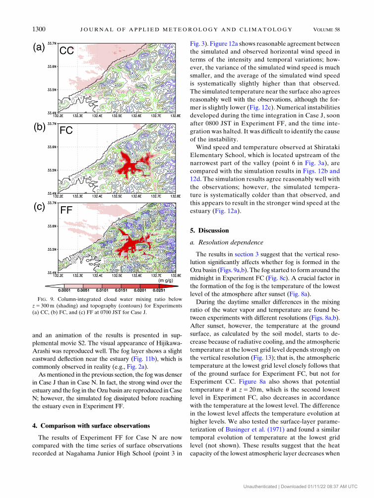
The amount of fog in theOzu basin varied little between

Experiments FC and FF (Figs. 9b,c); however, a significant

difference is found near the estuary: the fog was blocked

by the unrealistic saddle in the valley in Experiment FC

(Fig. 9b), whereas it flowed through the valley and reached

the sea in Experiment FF (Fig. 9c). A previous simulation

using CReSS with a coarser horizontal resolution of

300m (Nagoshi et al. 2013) gave results similar to those

of Experiment FC.

A three-dimensional visualization of simulated cloud

water mixing ratio for Experiment FF is shown in Fig. 11,

FIG. 8. Time series of (a) potential temperature u, (b) water vapor

qy , and (c) cloud water mixing ratio qc at heights of 5 and 20m at the

center of the Ozu basin where the AMeDAS station (Ozu) is located

(point 8 in Fig. 3a) for various experiments for Case J.

JUNE 2019 I TO ET AL . 1299

Unauthenticated | Downloaded 01/11/22 08:37 AM UTC

and an animation of the results is presented in sup-

plemental movie S2. The visual appearance of Hijikawa-

Arashi was reproduced well. The fog layer shows a slight

eastward deflection near the estuary (Fig. 11b), which is

commonly observed in reality (e.g., Fig. 2a).

Asmentioned in the previous section, the fog was denser

in Case J than in Case N. In fact, the strong wind over the

estuary and the fog in theOzubasin are reproduced inCase

N; however, the simulated fog dissipated before reaching

the estuary even in Experiment FF.

4. Comparison with surface observations

The results of Experiment FF for Case N are now

compared with the time series of surface observations

recorded at Nagahama Junior High School (point 3 in

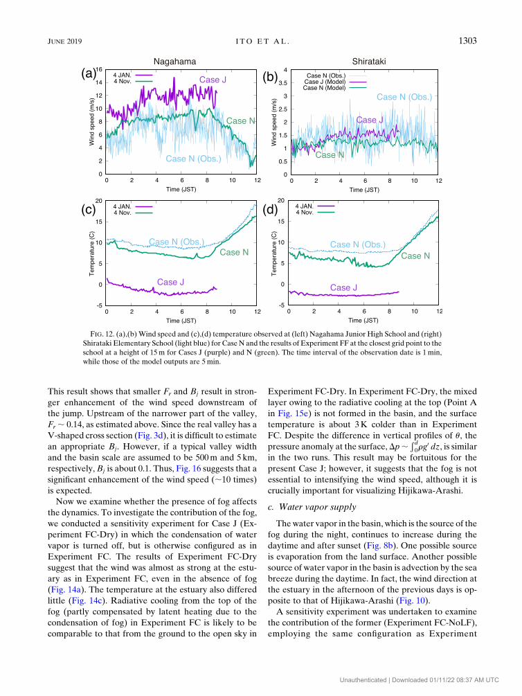
Fig. 3). Figure 12a shows reasonable agreement between

the simulated and observed horizontal wind speed in

terms of the intensity and temporal variations; how-

ever, the variance of the simulated wind speed is much

smaller, and the average of the simulated wind speed

is systematically slightly higher than that observed.

The simulated temperature near the surface also agrees

reasonably well with the observations, although the for-

mer is slightly lower (Fig. 12c). Numerical instabilities

developed during the time integration in Case J, soon

after 0800 JST in Experiment FF, and the time inte-

gration was halted. It was difficult to identify the cause

of the instability.

Wind speed and temperature observed at Shirataki

Elementary School, which is located upstream of the

narrowest part of the valley (point 6 in Fig. 3a), are

compared with the simulation results in Figs. 12b and

12d. The simulation results agree reasonably well with

the observations; however, the simulated tempera-

ture is systematically colder than that observed, and

this appears to result in the stronger wind speed at the

estuary (Fig. 12a).

5. Discussion

a. Resolution dependence

The results in section 3 suggest that the vertical reso-

lution significantly affects whether fog is formed in the

Ozu basin (Figs. 9a,b). The fog started to form around the

midnight in Experiment FC (Fig. 8c). A crucial factor in

the formation of the fog is the temperature of the lowest

level of the atmosphere after sunset (Fig. 8a).

During the daytime smaller differences in the mixing

ratio of the water vapor and temperature are found be-

tween experiments with different resolutions (Figs. 8a,b).

After sunset, however, the temperature at the ground

surface, as calculated by the soil model, starts to de-

crease because of radiative cooling, and the atmospheric

temperature at the lowest grid level depends strongly on

the vertical resolution (Fig. 13); that is, the atmospheric

temperature at the lowest grid level closely follows that

of the ground surface for Experiment FC, but not for

Experiment CC. Figure 8a also shows that potential

temperature u at z5 20m, which is the second lowest

level in Experiment FC, also decreases in accordance

with the temperature at the lowest level. The difference

in the lowest level affects the temperature evolution at

higher levels. We also tested the surface-layer parame-

terization of Businger et al. (1971) and found a similar

temporal evolution of temperature at the lowest grid

level (not shown). These results suggest that the heat

capacity of the lowest atmospheric layer decreases when

FIG. 9. Column-integrated cloud water mixing ratio below

z5 300m (shading) and topography (contours) for Experiments

(a) CC, (b) FC, and (c) FF at 0700 JST for Case J.

1300 JOURNAL OF APPL IED METEOROLOGY AND CL IMATOLOGY VOLUME 58

Unauthenticated | Downloaded 01/11/22 08:37 AM UTC

the vertical grid size is decreased; consequently, given the

heat flux at the ground surface, the atmospheric tem-

perature follows more closely that of the ground surface.

The evolution of the radiation fog after its formation

seems to be similar to that reported by Nakanishi (2000).

The fog at z5 5m appears prior to that at z5 20m

(Fig. 8c). Once the fog forms just above the ground, up-

ward longwave radiation from the top of the fog layer

causes active convection in the layer and effectively cools

the temperature of the whole layer, even in the presence

of warming, because of the release of latent heat. After

the fog started to develop in Experiment FC at 0000 JST

4 January, the temperature of the lowest atmospheric

level actually decreased further by 2K (Fig. 13). On the

other hand, the temperature of the ground started to

increase soon after the fog formed, probably because of

the downward longwave radiation from the fog.

Although we did not carry out surface observations

for Case J, surface temperature data from the AMeDAS

station at the center of the Ozu basin are available. The

observed time series of surface temperature indeed

continued to decrease after sunset (Fig. 13) and is more

consistent with the simulated temperature for Experi-

ment FC than for Experiment CC.

We conducted an additional experiment in which only

the resolution at the lowest level for Experiment CC is

improved from 40 to 10m while the number of vertical

levels is kept at 60. The result of this experiment (not

shown) indicates that the fine resolution at the lowest

level is particularly important for the fog near the surface.

Figure 14 compares the wind speed and surface tem-

perature at the estuary among Experiments CC, FC, and

FF. For both Cases J and N, the wind speed is strongest

in Experiment FF. The wind speeds at the estuary are

significantly different between Experiments FC and FF,

although the temperature differs little (Fig. 14). Two

possible reasons for the greater wind speed in Experi-

ment FF may be considered: first, the finer topography

can resolve the narrow valley, which is likely to result

in a higher wind speed (see the following subsection);

second, the bottom boundaries of some grid cells on the

Hijikawa River in Experiment FF are classified as

water surface, which has weaker friction than land and

thus contributes to the higher wind speed (Fig. 5b).

b. Dynamics

As mentioned in section 1, the enhancement of sur-

face wind speed downstream of the narrow valley

FIG. 10. Potential temperature (shading), the height with cloud water mixing ratio larger than 0.01 g kg21 (white

hatching), and horizontal wind speeds (wind barbs) in a time–height cross section (a),(c) at the estuary (Nagahama)

and (b),(d) in the basin (Ozu) for (top) Case J and (bottom) Case N in Experiment FC. Note that the ranges of the

shading are different between the top and bottom panels.

JUNE 2019 I TO ET AL . 1301

Unauthenticated | Downloaded 01/11/22 08:37 AM UTC

appears to be associated with a supercritical hydraulic

flow.The cold air in the basin flows out along theHijikawa

River while it accelerates and reduces its layer thickness

(Fig. 15a; the time evolution is shown in Figs. 15d,e, and

supplemental movie S3).

The flow depicted in Fig. 15 is not simple. At least two

jumps accompanying increases in the layer depth of the

cold air appear to occur along the final 5 km of the river.

As seen from movie S3, these jumps occur at fixed lo-

cations and remain stationary. The first jump occurs

downstream of the narrowest point of the valley (J1 in

Fig. 15a). Downstream of the narrowest point, the width

of the valley increases near Yamatobshi Bridge (point 5

in Fig. 3) where a tributary joins the Hijikawa River.

Then another jump occurs at the estuary (J2 in Fig. 15a).

Two obvious increases in surface wind speed along the

Hijikawa River are indeed found upstream of the jumps

(Fig. 15b). Multiple hydraulic jumps over a longer dis-

tance have been reported for a gap wind inHowe Sound,

British Columbia (Finnigan et al. 1994).

The temperature deficit Du of the cold airmass up-

stream of the narrowest point (point A in Fig. 15d)

with respect to the air over the sea is about 12K, and

the thickness of the cold air mass d is about 450m.

This induces a positive hydrostatic pressure anomaly

Dp; rg0d; 140 Pa, where g0 [ g(Du/u0) is the reduced

gravity, g is gravitational acceleration, u0 is the standard

temperature, and r is the density of the air. This hy-

drostatic pressure anomaly is comparable to the differ-

ence in the simultaneously observed sea level pressure

between the basin and estuary, as reported by Ohashi

et al. (2015).

The Froude number (Fr [ u/ffiffiffiffiffiffiffig0d

p) at point A is es-

timated as ;0.14 (u ; 2m s21), which is subcritical. In

the area between the two jumps (e.g., point B in Fig. 15,

where u ; 11m s21 and d ; 205m), Fr ; 1.06, which is

slightly supercritical. At the estuary (point C in Fig. 15,

where u ; 14m s21 and d ; 50m), Fr ; 3.16, which is

supercritical.

Since a clear capping inversion exists above the cold

air (Fig. 15d), it is of interest to apply a theoretical

analysis of a two-layer flow, which is analogous to shal-

low water theory. Saito (1992) studied shallow water

flow over a saddle-shaped topography and reported a

regime with a stationary hydraulic jump. Following

Saito (1992), we seek a solution for a stationary hydro-

static jump in a two-layer flow over a channel, although

Hijikawa-Arashi in reality is much more complex than

assumed in the theory (e.g., multiple jumps as men-

tioned above, surface friction, and a V-shaped valley

as seen in Fig. 3d). Using the notation of Saito (1992),

the system of governing equations may be written as

follows:

u2i

2g01 h

i5

u22

2g01h

2, (1)

u2d

2g01 h

d5

u21

2g01 h

1, (2)

hiuib05 h

2u2bj5 h

1u1bj5h

dudb0, and (3)

u25

ffiffiffiffiffiffiffiffiffiffiffiffiffiffiffiffiffiffiffiffiffiffiffiffiffiffiffiffih1

h2

g0h21 h

1

2

s, (4)

where hi and ui are the height and velocity of the cold

air upstream of the narrow part, respectively; h2 and u2

are those upstream of a jump, and h1 and u1 are those

downstream of a jump; hd and ud are those far down-

stream; and bo and bj are channel widths upstream and

at the jump, respectively. After nondimensionalization,

the above system for 6 equations with 10 unknowns

is shown to be governed by two nondimensional num-

bers (Buckingham p theorem): the Froude number

Fr [ ui/ffiffiffiffiffiffiffiffig0hi

pin the far upstream and the ratio of

the channel width at the jump to upstream Bj [ bj/b0.

The solution also must satisfy the critical condition

11 0:5F2r 2 1:5(Fr/Bj)

(2/3)# 0 (Long 1953).

Figure 16 shows the enhanced wind speed upstream of

the jump u2/u0 over the parameter space of Fr and Bj.

FIG. 11. Three-dimensional visualization of the simulated Hiji-

kawa-Arashi for Experiment FF for Case J: (a) looking north, with

the estuary at the upper right; (b) looking south from the estuary.

1302 JOURNAL OF APPL IED METEOROLOGY AND CL IMATOLOGY VOLUME 58

Unauthenticated | Downloaded 01/11/22 08:37 AM UTC

This result shows that smaller Fr and Bj result in stron-

ger enhancement of the wind speed downstream of

the jump. Upstream of the narrower part of the valley,

Fr ; 0.14, as estimated above. Since the real valley has a

V-shaped cross section (Fig. 3d), it is difficult to estimate

an appropriate Bj. However, if a typical valley width

and the basin scale are assumed to be 500m and 5km,

respectively, Bj is about 0.1. Thus, Fig. 16 suggests that a

significant enhancement of the wind speed (;10 times)

is expected.

Now we examine whether the presence of fog affects

the dynamics. To investigate the contribution of the fog,

we conducted a sensitivity experiment for Case J (Ex-

periment FC-Dry) in which the condensation of water

vapor is turned off, but is otherwise configured as in

Experiment FC. The results of Experiment FC-Dry

suggest that the wind was almost as strong at the estu-

ary as in Experiment FC, even in the absence of fog

(Fig. 14a). The temperature at the estuary also differed

little (Fig. 14c). Radiative cooling from the top of the

fog (partly compensated by latent heating due to the

condensation of fog) in Experiment FC is likely to be

comparable to that from the ground to the open sky in

Experiment FC-Dry. In Experiment FC-Dry, the mixed

layer owing to the radiative cooling at the top (Point A

in Fig. 15e) is not formed in the basin, and the surface

temperature is about 3K colder than in Experiment

FC. Despite the difference in vertical profiles of u, the

pressure anomaly at the surface, Dp;Ð d0rg0 dz, is similar

in the two runs. This result may be fortuitous for the

present Case J; however, it suggests that the fog is not

essential to intensifying the wind speed, although it is

crucially important for visualizing Hijikawa-Arashi.

c. Water vapor supply

Thewater vapor in the basin, which is the source of the

fog during the night, continues to increase during the

daytime and after sunset (Fig. 8b). One possible source

is evaporation from the land surface. Another possible

source of water vapor in the basin is advection by the sea

breeze during the daytime. In fact, the wind direction at

the estuary in the afternoon of the previous days is op-

posite to that of Hijikawa-Arashi (Fig. 10).

A sensitivity experiment was undertaken to examine

the contribution of the former (Experiment FC-NoLF),

employing the same configuration as Experiment

FIG. 12. (a),(b) Wind speed and (c),(d) temperature observed at (left) Nagahama Junior High School and (right)

Shirataki Elementary School (light blue) for CaseN and the results of Experiment FF at the closest grid point to the

school at a height of 15m for Cases J (purple) and N (green). The time interval of the observation date is 1min,

while those of the model outputs are 5min.

JUNE 2019 I TO ET AL . 1303

Unauthenticated | Downloaded 01/11/22 08:37 AM UTC

FC except that the soil water is set to zero throughout

the time integration. The NWP model prescribes the

surface water vapor flux from the land to the atmo-

sphere by considering the soil water budget. There-

fore, the surface water vapor fluxes from the land only

are eliminated.

As a result of reduced vapor supply from the land, the

amount of cloud water corresponding to the fog in the

lower atmosphere in Case J is significantly decreased

(Figs. 9b and 17). Nevertheless, the wind speed and

temperature at the estuary vary little between Experi-

ment FC and Experiment FC-NoLF (Figs. 14a,c), which

is consistent with the results of Experiment FC-Dry.

Figure 8b shows that the water vapor mixing ratio in

the basin in Experiment FC-NoLF increases in almost

the same manner as in Experiment FC during the day-

time, and this suggests that advection by sea breezes is

also important. Furthermore, the difference between

Experiments FC and FC-NoLF becomes larger after

sunset (after 1600 JST in Fig. 8b). Nocturnal katabatic

valley winds (e.g., Whiteman 1990) from various valleys

converge at the center of the basin, and contribute to the

accumulation of water vapor. In Experiment FC-NoLF,

the katabatic winds are drier because of the absence of

the water vapor flux from the land surface.

Another sensitivity experiment was conducted (Ex-

periment FC-NoSea), employing the same configuration

as Experiment FC except that the sea surface in a square

of about 100 km 3 100 km around the estuary of the

Hijikawa River is changed to the land (Fig. 18a). As a

result, the cloud water in the basin in the next morning

almost disappears in Experiment FC-NoSea (Fig. 18b).

FIG. 14. (a),(b) Wind speed and (c),(d) temperature observed at Nagahama Junior High School (estuary) for (left)

Case J and (right) Case N for various configurations of numerical experiments.

FIG. 13. Time series of atmospheric temperature at the lowest

grid level (solid lines) and the ground surface temperature (dashed

lines) for Experiments CC (purple) and FC (green) for Case J at

the center of the Ozu basin. Hourly data recorded at the AMeDAS

station (Ozu) are shown by light blue dots.

1304 JOURNAL OF APPL IED METEOROLOGY AND CL IMATOLOGY VOLUME 58

Unauthenticated | Downloaded 01/11/22 08:37 AM UTC

This result confirms the daytime sea breeze substantially

contributes to the water vapor supply.

d. Enhanced thermal contrast

This subsection clarifies that the sea has another role in

addition to the water vapor supply. The configuration of

Experiment FC-NoSea exhibited in the previous sub-

section is similar to other thermally driven gap winds

for which a small basin is connected to a larger basin

through a narrow valley. Now, the ground surface tem-

perature decreases in the night because of radiative

cooling on the drained land in Experiment FC-NoSea.

The ground surface temperature in the basin is about

270K in the morning of Case J, and SST of the Seto

Inland Sea is almost fixed to be 287K. Whereas, in Exper-

iment FC-NoSea, that of the drained land is 277K.

Figure 18c shows surface wind speed around the es-

tuary of the Hijikawa River in Experiment FC-NoSea.

The gap wind indeed occurs by virtue of the character-

istic topography. However, compared with Experiment

FC (Fig. 7b), the surface wind speed associated with

the gap wind is about 2m s21 weaker. This deceleration

appears to be caused by the smaller thermal contrast in

the absence of the sea. These results show thatHijikawa-

Arashi is driven by the horizontal gradient of hydrostatic

pressure between theOzu basin and the Seto Inland Sea.

The pressure tends to be higher in the Ozu basin where

the downslope winds along the radiatively cooled sur-

rounding slopes and compensating adiabatic ascents in

the center accumulate cold air effectively. The warm

air caused by the SST over the sea also contributes to

increase the horizontal pressure gradient.

6. Conclusions

Hijikawa-Arashi, a thermally driven gap wind that

occurs in the northwestern part of Shikoku Island in

Japan during the cold season, was reproduced reason-

ably well by a NWP model with fine horizontal (80m)

and vertical resolution (;10m near the surface). Al-

though it is not usual to employ such a fine resolution

in a NWP model, the present study demonstrated its

potential in simulating microscale meteorological phe-

nomena. Simulated temporal variations in temperature

and wind speed agree reasonably well with those ob-

served at surface stations. Even the fog layer flowing out

over the Seto Inland Sea from the estuary, which is one

of the unique features ofHijikawa-Arashi, is reproduced

for one case.

Fine vertical resolution near the surface is essential

in simulating a realistic cooling of the lower atmo-

sphere after sunset and fog formation in the Ozu basin.

FIG. 16. Enhancement of flow speed upstream of a hydraulic

jump u2/u0 over the parameter space of the Froude number Fr and

the ratio of the channel width at the jump to upstreamBj predicted

by the analytic solution of a two-layer flow.

FIG. 15. (a) Potential temperature (shading) and wind vectors,

and (b) horizontal wind velocity at 10m AGL (positive to the left)

along the red dotted line shown in (c) that shows topography by

shading. The locations of two jumps are indicated as J1 and J2 in

(a). The narrowest point in the valley is marked by the cross in (c),

and vertical profiles of potential temperature and horizontal

velocity, at points A, B, and C in (c), are shown in (d) and (e),

respectively.

JUNE 2019 I TO ET AL . 1305

Unauthenticated | Downloaded 01/11/22 08:37 AM UTC

At coarse vertical resolution, the temperature of the lower

atmosphere is less affected by that of the land surface. This

issue is likely to commonly arise when nocturnal stable

boundary layers are simulated in NWP models.

The successful numerical simulation clarifies the dy-

namics and environmental features of Hijikawa-Arashi.

The temperature contrast of 10K or more between the

air over the sea and that in the Ozu basin develops be-

cause of nighttime radiative cooling of the land. The

strong wind at the estuary is caused by the outflow of

cold air that accumulated over the Ozu basin and is en-

hanced by the narrow gap in the valley of the Hijikawa

River. Detailed features of Hijikawa-Arashi were

also simulated well; for example, two distinct hydraulic

jumps occur, one just downstream of the narrowest part

of the valley and the other at the estuary; and the river

surface with relatively low surface friction helps to

form the strong wind.

Water vapor provided by the daytime sea breeze and

evaporation from the land surface seem to be important

in forming the fog in the Ozu basin. Although the fog is

important for visualizing the wind, it may not be critical

to the dynamics. The wind of the same strength can

occur in an environment with less water vapor supplies

owing to the characteristic topography.

The present resolution may be insufficient to simulate

steam fog observed on the surface of water bodies (e.g.,

Fig. 2b) and that takes the formof longitudinal rolls, which

is a preferred pattern of thermal convection in the pres-

ence of a strong vertical shear (Asai 1970). An additional

issue concerning steam fog is the temperature of the water

surface, as no high-resolution data of sea surface tem-

perature in the Seto Inland Sea were available for the

present simulation. Furthermore, no data were available

for the river surface temperature, so that we tentatively

employed the SST of the nearby sea in its place.

FIG. 18. (a) Topography and coast lines (white), (b) column-

integrated cloud water mixing ratio below z5 300m (shading) as

in Fig. 9, and (c) surface wind vectors (arrows) and magnitude

(shading) as in Fig. 7 in Experiment FC-NoSea.

FIG. 17. As in Fig. 9b, but for Experiment FC-NoLF in which soil

water is eliminated.

1306 JOURNAL OF APPL IED METEOROLOGY AND CL IMATOLOGY VOLUME 58

Unauthenticated | Downloaded 01/11/22 08:37 AM UTC

The enhancement of the wind at the estuary is rela-

tively easy to predict with a NWP model. In fact, it was

even reproduced in Experiment CC when no fog was

formed for Case J. Since Hijikawa-Arashi visualized by

fog is an important tourist attraction, its prediction may

be useful for tourists. We have shown that finer hori-

zontal and vertical resolutions, realistic topography,

and details of land use are necessary for its accurate

prediction. Furthermore, reliable representation of tur-

bulent diffusion seems to be important in predicting

whether the fog is advected to the estuary or dissipated

along its path. This remains a topic to be studied in

the future.

Acknowledgments. We thank Masaru Kurosaka for

surface observations, Yukitaka Ohashi for useful discus-

sions, and three anonymous reviewers for their helpful

comments. This workwas supported by JSPSKAKENHI

Grants 26800244, 17K04837, 26350181, and 23501000,

and by the Advancement of Meteorological and Global

Environmental Predictions Utilizing Observational Big

Data of the Social and Scientific Priority Issues (Theme 4)

to be tackled by using the post K computer of the

FLAGSHIP 2020 Project.

REFERENCES

Asai, T., 1970: Stability of a plane parallel flow with variable ver-

tical shear and unstable stratification. J. Meteor. Soc. Japan,

48, 129–139, https://doi.org/10.2151/jmsj1965.48.2_129.

Banta, R. M., L. S. Darby, J. D. Fast, J. O. Pinto, C. D. Whiteman,

W. J. Shaw, and B. W. Orr, 2004: Nocturnal low-level jet in a

mountain basin complex. Part I: Evolution and effects on local

flows. J. Appl. Meteor., 43, 1348–1365, https://doi.org/10.1175/JAM2142.1.

Beljaars, A. C. M., and A. A. M. Holtslag, 1991: Flux parameteriza-

tion over land surfaces for atmospheric models. J. Appl.Meteor.,

30, 327–341, https://doi.org/10.1175/1520-0450(1991)030,0327:

FPOLSF.2.0.CO;2.

Businger, J. A., J. C. Wyngaard, Y. Izumi, and E. F. Bradley,

1971: Flux-profile relationships in the atmospheric surface

layer. J. Atmos. Sci., 28, 181–189, https://doi.org/10.1175/1520-0469(1971)028,0181:FPRITA.2.0.CO;2.

Chrust, M. F., C. D. Whiteman, and S. W. Hoch, 2013: Observa-

tions of thermally driven wind jets at the exit of Weber Can-

yon, Utah. J. Appl. Meteor. Climatol., 52, 1187–1200, https://

doi.org/10.1175/JAMC-D-12-0221.1.

Deardorff, J.W., 1980: Stratocumulus-cappedmixed layers derived

from a three-dimensional model. Bound.-Layer Meteor., 18,495–527, https://doi.org/10.1007/BF00119502.

Finn, D., and Coauthors, 2016: Evidence for gap flows in the Birch

Creek Valley, Idaho. J. Atmos. Sci., 73, 4873–4894, https://

doi.org/10.1175/JAS-D-16-0052.1.

Finnigan, T. D., J. A. Vine, P. L. Jackson, S. E. Allen, G. A.

Lawrence, andD.G. Steyn, 1994:Hydraulic physicalmodeling

and observations of a severe gap wind. Mon. Wea. Rev., 122,

2677–2687, https://doi.org/10.1175/1520-0493(1994)122,2677:

HPMAOO.2.0.CO;2.

Liu, M., D. L. Westphal, T. R. Holt, Q. Xu, M. Liu, D. L. Westphal,

T.R.Holt, andQ.Xu, 2000:Numerical simulation of a low-level

jet over complex terrain in southern Iran.Mon. Wea. Rev., 128,

1309–1327, https://doi.org/10.1175/1520-0493(2000)128,1309:

NSOALL.2.0.CO;2.

Long, R. R., 1953: Some aspects of the flow of stratified fluids: I. A

theoretical investigation. Tellus, 5, 42–58, https://doi.org/

10.3402/tellusa.v5i1.8563.

Mayr, G. J., and Coauthors, 2007: Gap flows: Results from the

Mesoscale Alpine Programme. Quart. J. Roy. Meteor. Soc.,

133, 881–896, https://doi.org/10.1002/qj.66.

Nagoshi, T., 2009: Teaching materials on a fluid experiment of the

local wind by using a solid relief model of geographical fea-

tures: A case study of Hijikawa Arashi, a kind of land breeze

with fogs. Educ. Earth Sci., 62, 65–76.

——, S. Saito, S. Inoue, M. Yoshioka, M. Kato, and K. Tsuboki,

2013: Numerical simulation of fog in ‘‘Hijikawa-Arashi’’

using a cloud resolving model ‘‘DVD-CReSS’’ (in Japanese).

Proc. Meteorological Society of Japan Autumn Meeting,

Sendai, Japan, Meteorological Society of Japan, D117.

Nakanishi, M., 2000: Large-eddy simulation of radiation fog.

Bound.-Layer Meteor., 94, 461–493, https://doi.org/10.1023/

A:1002490423389.

Ohashi, Y., T. Terao, Y. Shigeta, and T. Ohsawa, 2015: In situ

observational research of the gap wind ‘‘Hijikawa-arashi’’

in Japan. Meteor. Atmos. Phys., 127, 33–48, https://doi.org/

10.1007/s00703-014-0345-1.

——, T. Katsuta, H. Tani, T. Okabayashi, S. Miyahara, and

R. Miyashita, 2018: Human cold stress of strong local-wind

‘‘Hijikawa-arashi’’ in Japan, based on the UTCI index and

thermo-physiological responses. Int. J. Biometeor., 62, 1241–

1250, https://doi.org/10.1007/s00484-018-1529-z.

Saito, K., 1992: Shallow water flow having a lee hydraulic jump

over a mountain range in a channel of variable width.

J. Meteor. Soc. Japan, 70, 775–782, https://doi.org/10.2151/

jmsj1965.70.3_775.

——, and Coauthors, 2006: The operational JMA nonhydrostatic

mesoscale model. Mon. Wea. Rev., 134, 1266–1298, https://

doi.org/10.1175/MWR3120.1.

Shigeta, Y., 2009: Numerical simulation and observation of

Hijikawa-arashi. Proc. Meteorological Society of JapanAutumn

Meeting, Vol. 96, Fukuoka, Japan, Meteorological Society of

Japan, D306, http://ci.nii.ac.jp/naid/110007626680/.

Tsuboki, K., and A. Sakakibara, 2002: Large-scale parallel com-

puting of cloud resolving storm simulator. High Performance

Computing: ISHPC 2002, H. P. Zima et al., Eds., Lecture

Notes in Computer Science, Vol 2327, Springer, 243–259.

Wagenbrenner, N., J. Forthofer, C. Gibson,A. Indreland, B. Lamb,

and B. Butler, 2018: Observations and predictability of gap

winds in the Salmon River Canyon of central Idaho, USA.

Atmosphere, 9, 45, https://doi.org/10.3390/atmos9020045.

Whiteman, C. D., 1990: Observations of thermally developed wind

systems in mountainous terrain. Atmospheric Processes over

Complex Terrain, W. Blumen, Ed., Amer. Meteor. Soc., 5–42.

Zängl, G., 2004: A reexamination of the valley wind system in the

Alpine Inn Valley with numerical simulations.Meteor. Atmos.

Phys., 87, 241–256, https://doi.org/10.1007/s00703-003-0056-5.

JUNE 2019 I TO ET AL . 1307

Unauthenticated | Downloaded 01/11/22 08:37 AM UTC

CORRIGENDUM

JUNSHI ITO,a TOSHIYUKI NAGOSHI,b AND HIROSHI NIINOc

aGraduate School of Science, Tohoku University, Sendai, Miyagi, Japanb Iwate University, Morioka, Iwate, Japan

cAtmosphere and Ocean Research Institute, The University of Tokyo, Kashiwa, Chiba, Japan

(Manuscript received 5 May 2021, in final form 20 May 2021)

Figure 15 in Ito et al. (2019) did not include two panels, Figs. 15d and 15e, that werementioned in the

text and caption, and labels indicating points A, B, and C in Fig. 15c were not properly placed. The

corrected figure is presented here. The errors do not affect the results and discussion.

We regret that these mistakes occurred during the preparation of the final typescript and were

overlooked through proofreading. The authors apologize for any inconvenience.

Acknowledgments. Authors thank Professor Yukitaka Ohashi for pointing out the mistake.

REFERENCES

Ito, J., T. Nagoshi, andH. Niino, 2019: A numerical study of ‘‘Hijikawa-Arashi’’: A thermally driven gap wind

visualized by nocturnal fog. J. Appl. Meteor. Climatol., 58, 1293–1307, https://doi.org/10.1175/JAMC-D-

18-0189.1.

Corresponding author: Junshi Ito, junshi@tohoku.ac.jp

JUNE 2021 CORR IGENDUM 873

DOI: 10.1175/JAMC-D-21-0086.1

� 2021 American Meteorological Society. For information regarding reuse of this content and general copyright information, consult the AMS CopyrightPolicy (www.ametsoc.org/PUBSReuseLicenses).

Unauthenticated | Downloaded 01/11/22 08:37 AM UTC

FIG. 15. (a) Potential temperature (shading) and wind vectors

and (b) horizontal wind velocity at 10 m AGL (positive to the left)

along the red dotted line shown in (c) a plot of the valley of interest,

in which the topography is shown by shading. The locations of two

jumps are indicated as J1 and J2 in (a). The narrowest point in the

valley is marked by the cross in (c). Also shown are vertical profiles

of (d) potential temperature and (e) horizontal velocity at points

A, B, and C in (c).

874 JOURNAL OF APPL IED METEOROLOGY AND CL IMATOLOGY VOLUME 60

Unauthenticated | Downloaded 01/11/22 08:37 AM UTC