a novel signal processing method for intraoperative

Florida International UniversityFIU Digital Commons

FIU Electronic Theses and Dissertations University Graduate School

11-15-2013

A Novel Signal Processing Method forIntraoperative Neurophysiological Monitoring inSpinal SurgeriesKrishnatej VedalaFlorida International University, [email protected]

Follow this and additional works at: http://digitalcommons.fiu.edu/etd

Part of the Bioelectrical and Neuroengineering Commons, Biomedical Commons, BiomedicalDevices and Instrumentation Commons, Neurosciences Commons, Other Neuroscience andNeurobiology Commons, Signal Processing Commons, and the Surgical Procedures, OperativeCommons

This work is brought to you for free and open access by the University Graduate School at FIU Digital Commons. It has been accepted for inclusion inFIU Electronic Theses and Dissertations by an authorized administrator of FIU Digital Commons. For more information, please contact [email protected].

Recommended CitationVedala, Krishnatej, "A Novel Signal Processing Method for Intraoperative Neurophysiological Monitoring in Spinal Surgeries" (2013).FIU Electronic Theses and Dissertations. Paper 1038.http://digitalcommons.fiu.edu/etd/1038

http://digitalcommons.fiu.edu?utm_source=digitalcommons.fiu.edu%2Fetd%2F1038&utm_medium=PDF&utm_campaign=PDFCoverPages

http://digitalcommons.fiu.edu/etd?utm_source=digitalcommons.fiu.edu%2Fetd%2F1038&utm_medium=PDF&utm_campaign=PDFCoverPages

http://digitalcommons.fiu.edu/ugs?utm_source=digitalcommons.fiu.edu%2Fetd%2F1038&utm_medium=PDF&utm_campaign=PDFCoverPages

http://digitalcommons.fiu.edu/etd?utm_source=digitalcommons.fiu.edu%2Fetd%2F1038&utm_medium=PDF&utm_campaign=PDFCoverPages

http://network.bepress.com/hgg/discipline/231?utm_source=digitalcommons.fiu.edu%2Fetd%2F1038&utm_medium=PDF&utm_campaign=PDFCoverPages










http://digitalcommons.fiu.edu/etd/1038?utm_source=digitalcommons.fiu.edu%2Fetd%2F1038&utm_medium=PDF&utm_campaign=PDFCoverPages

mailto:[email protected]

FLORIDA INTERNATIONAL UNIVERSITY

Miami, Florida

A NOVEL SIGNAL PROCESSING METHOD FOR INTRAOPERATIVE

NEUROPHYSIOLOGICAL MONITORING IN SPINAL SURGERIES

A dissertation submitted in partial fulfillment of the

requirements for the degree of

DOCTOR OF PHILOSOPHY

in

ELECTRICAL ENGINEERING

by

Krishnatej Vedala

2013

To: Dean Amir MirmiranCollege of Engineering and Computing

This dissertation, written by Krishnatej Vedala, and entitled A Novel Signal Process-ing Method for Intraoperative Neurophysiological Monitoring in Spinal Surgeries,having been approved in respect to style and intellectual content, is referred to youfor judgment.

We have read this dissertation and recommend that it be approved.

Armando Barreto

Jean Andrian

Naphtali Rishe

Malek Adjouadi, Major Professor

Date of Defense: November 15, 2013

The dissertation of Krishnatej Vedala is approved.

Dean Amir MirmiranCollege of Engineering and Computing

Dean Lakshmi N. ReddiUniversity Graduate School

Florida International University, 2013

ii

© Copyright 2013 by Krishnatej Vedala

All rights reserved.

iii

DEDICATION

I dedicate this dissertation to my wonderful parents and my sister.

iv

ACKNOWLEDGMENTS

This dissertation has been made possible by the collective support of my family,

friends and mentors. I would like to thank my parents and my sister who are my

greatest support system in life. Their unconditional love and support have kept me

going through the hard times.

My mentor Dr. Malek Adjouadi has taught me a great deal in professional, personal

and intellectual development. He has always had my best interest at heart and has

provided me with every opportunity to grow. I am grateful for all the kindness and

patience that he has shown me over the years. I would like to thank my gurus, Dr.

Armando Barreto, Dr. Jean Andrian and Dr. Naphtalie Rishe, naming a few, whose

interaction gave me new insights to my research work.

I would also like to thank our collaborators Dr. Ilker Yaylali and Dr. Melvin Ayala

for their invaluable advice and directions. My thanks also go to my colleages at

Center for Advanced Technology and Education (CATE) Dr. Mercedes Cabrerizo,

Dr. Mohammed Goryawala, Dr. Changan Han, Dr. Jin Wang, Dr. Yu Chen and

many more current and former members for their many useful suggestions.

I would also like to thank the members of the Electrical Engineering Department,

Mr. Oscar Silveira, Ms. Pat Brammer and Ms. Ana Saenz and Ms. Maria Benincasa

from the School of Engineering for the support throughout the course of my studies

and the laughs we have shared.

I would like to express my special thanks to my friends around the globe. They have

come and gone but each one leaving a permanent impression in my life in a special

v

way and taught me to live life to the fullest. Their support and good wishes have

been the driving force in helping me successfully finish my dissertation.

vi

ABSTRACT OF THE DISSERTATION

A NOVEL SIGNAL PROCESSING METHOD FOR INTRAOPERATIVE

NEUROPHYSIOLOGICAL MONITORING IN SPINAL SURGERIES

by

Krishnatej Vedala

Florida International University, 2013

Miami, Florida

Professor Malek Adjouadi, Major Professor

Intraoperative neurophysiologic monitoring (IONM) is an integral part of spinal

surgeries and involves the recording of somatosensory evoked potentials (SSEP).

However, clinical application of IONM still requires anywhere between 200 to 2000

trials to obtain an SSEP signal, which is excessive and introduces a significant

delay to prevent potential neurological risks during surgery. The main objective

of this dissertation is to develop a means to obtain the SSEP signal using a much

reduced number of trials (20 trials or less) while still optimizing the effectiveness

of the monitoring system. The preliminary research steps were to determine those

characteristics that distinguish the SSEP with the ongoing brain activity. We first

established that the brain activity is indeed quasi-stationary whereas an SSEP is

expected to be identical every time a trial is recorded.

A novel algorithm is subsequently developed using Chebyshev time windowing for

preconditioning of SSEP trials to retain the morphological characteristics of so-

matosensory evoked potentials (SSEP). This preconditioning was followed by the

application of a principal component analysis (PCA)-based algorithm utilizing quasi-

stationarity of EEG on 12 preconditioned trials. A unique Walsh transform opera-

tion was then used to identify the position of the SSEP event. An alarm is raised

vii

when there is a 10% time in latency deviation and/or 50% peak-to-peak amplitude

deviation, as per the clinical requirements. The algorithm shows consistency in the

results in monitoring SSEP in up to 6-hour surgical procedures even under this

significantly reduced number of trials.

In this study, the analysis was performed on the data recorded in 29 patients who

underwent surgery during which the posterior tibial nerve was stimulated and SSEP

response was recorded from scalp EEG. This method is shown empirically to be more

clinically viable than present day approaches. In all 29 cases, the algorithm took on

an average 4sec to extract an SSEP signal, as compared to conventional methods,

which take up to several minutes.

The monitoring process using the algorithm was successful and proved conclusive

under the clinical constraints throughout the different surgical procedures with an

accuracy of 91.5%. Higher accuracy and faster execution time, observed in the

present study, in determining the SSEP signals provided for a much improved and

effective neurophysiological monitoring process.

viii

TABLE OF CONTENTS

CHAPTER PAGE

1. INTRODUCTION . . . . . . . . . . . . . . . . . . . . . . . . . . . . . . . 11.1 Intraoperative Monitoring . . . . . . . . . . . . . . . . . . . . . . . . . . 11.2 Motivation . . . . . . . . . . . . . . . . . . . . . . . . . . . . . . . . . . . 21.3 Hypotheses . . . . . . . . . . . . . . . . . . . . . . . . . . . . . . . . . . 31.4 Research Questions . . . . . . . . . . . . . . . . . . . . . . . . . . . . . . 41.5 Significance of the study . . . . . . . . . . . . . . . . . . . . . . . . . . . 41.6 Literature Survey . . . . . . . . . . . . . . . . . . . . . . . . . . . . . . . 51.7 Database and Recordings . . . . . . . . . . . . . . . . . . . . . . . . . . 7

2. ALGORITHM VERSION 1 – EIGEN SPACE FILTERING . . . . . . . . 102.1 Background . . . . . . . . . . . . . . . . . . . . . . . . . . . . . . . . . . 102.2 Structure of the algorithm . . . . . . . . . . . . . . . . . . . . . . . . . . 112.3 Implementation . . . . . . . . . . . . . . . . . . . . . . . . . . . . . . . . 152.3.1 AMUSE algorithm – Noise components filtering . . . . . . . . . . . . . 232.3.2 Walsh transform – Automated peak detection . . . . . . . . . . . . . . 252.4 Implementation Results . . . . . . . . . . . . . . . . . . . . . . . . . . . 26

3. ALGORITHM VERSION 2 – TEMPORAL FILTERING . . . . . . . . . 373.1 Background . . . . . . . . . . . . . . . . . . . . . . . . . . . . . . . . . . 373.2 Gaussian Template . . . . . . . . . . . . . . . . . . . . . . . . . . . . . . 373.3 Chebyshev Filtering . . . . . . . . . . . . . . . . . . . . . . . . . . . . . 38

4. ALGORITHM VERSION 3 – COMBINATION OF EIGEN & TEMPORALFILTERING . . . . . . . . . . . . . . . . . . . . . . . . . . . . . . . . . . 44

4.1 Merits of Pre-filtering . . . . . . . . . . . . . . . . . . . . . . . . . . . . . 444.2 Implementation . . . . . . . . . . . . . . . . . . . . . . . . . . . . . . . . 444.2.1 Data Acquisition . . . . . . . . . . . . . . . . . . . . . . . . . . . . . . 444.2.2 Pre-filtering or Pre-conditioning . . . . . . . . . . . . . . . . . . . . . . 474.2.3 Eigen Space . . . . . . . . . . . . . . . . . . . . . . . . . . . . . . . . . 474.2.4 Reconstruction . . . . . . . . . . . . . . . . . . . . . . . . . . . . . . . 514.2.5 Information Extraction . . . . . . . . . . . . . . . . . . . . . . . . . . . 514.3 Results . . . . . . . . . . . . . . . . . . . . . . . . . . . . . . . . . . . . . 514.3.1 Implementation . . . . . . . . . . . . . . . . . . . . . . . . . . . . . . . 514.3.2 False Alarms . . . . . . . . . . . . . . . . . . . . . . . . . . . . . . . . 54

5. CONCLUSIONS AND FUTURE WORK . . . . . . . . . . . . . . . . . . 635.1 Conclusions from algorithm versions . . . . . . . . . . . . . . . . . . . . 635.1.1 Version 1 . . . . . . . . . . . . . . . . . . . . . . . . . . . . . . . . . . 635.1.2 Version 2 . . . . . . . . . . . . . . . . . . . . . . . . . . . . . . . . . . 645.1.3 Version 3 . . . . . . . . . . . . . . . . . . . . . . . . . . . . . . . . . . 66

ix

5.2 Discussion . . . . . . . . . . . . . . . . . . . . . . . . . . . . . . . . . . . 695.3 Future Study and Recommendations . . . . . . . . . . . . . . . . . . . . 715.3.1 Exhaustive study . . . . . . . . . . . . . . . . . . . . . . . . . . . . . . 715.3.2 Practical implementation . . . . . . . . . . . . . . . . . . . . . . . . . 71

REFERENCES . . . . . . . . . . . . . . . . . . . . . . . . . . . . . . . . . . 73

VITA . . . . . . . . . . . . . . . . . . . . . . . . . . . . . . . . . . . . . . . . 82

x

LIST OF TABLES

TABLE PAGE

2.1 Results of analysis from the implementation of algorithm of version 1 . . 274.1 Patient details and algorithm version 3 accuracy results . . . . . . . . . 484.2 Summary of the results from the implementation of the proposed algo-

rithm showing the average variability in the time latency and ampli-tude and the total number of false alarms raised for each patient. . . 57

4.3 Amplitude and time latency consistency for patient 10 from table 4.1 . . 595.1 Summary of results showing the average percentage error and percentage

deviation . . . . . . . . . . . . . . . . . . . . . . . . . . . . . . . . . 65

xi

LIST OF FIGURES

FIGURE PAGE

1.1 Screen-shot of CASCADE IONM system displaying SSEP extractedfrom four bi-polar electrodes. . . . . . . . . . . . . . . . . . . . . . . 8

2.1 Flowchart for the algorithm version 1 and the details of AMUSE algo-rithm are indicated by the arrow. . . . . . . . . . . . . . . . . . . . . 12

2.2 Comparison between algorithm version 1 and clinical implmentations . . 162.2 (cont.) . . . . . . . . . . . . . . . . . . . . . . . . . . . . . . . . . . . . . 172.3 Y1(n) - The ten components of the ten trials recorded, X1(n), from

the CZ–FZ channel and decomposed using AMUSE algorithm. TheX-axis represents the sampling time intervals. . . . . . . . . . . . . . 19

2.4 PSD of two components from fig. 2.3 . . . . . . . . . . . . . . . . . . . . 202.4 (cont.) . . . . . . . . . . . . . . . . . . . . . . . . . . . . . . . . . . . . . 212.5 Reconstruction of SSEP from high frequency and low frequency compo-

nents . . . . . . . . . . . . . . . . . . . . . . . . . . . . . . . . . . . 242.6 Significance of removing the low-frequency components . . . . . . . . . . 332.7 Application of Walsh transform to identify the position of the SSEP . . 342.8 Automated detection of evoked response from 10 trials. . . . . . . . . . 352.9 Consistency in detecting P37 and N45 peak latencies from the CZ–FZ

recording of subject 20 with the peak latencies (algorithm vs. clini-cal) as given in table 2.1d. . . . . . . . . . . . . . . . . . . . . . . . . 36

3.1 Outline of the SSEP recording timeline as compared with the clinicalmonitoring. By the time one clinical SSEP is obtained, the algorithmversion 2 obtained 10 SSEP signals. . . . . . . . . . . . . . . . . . . 41

3.2 Comparison of signals before and after applying Chebyshev filtering withthe actual average signal. . . . . . . . . . . . . . . . . . . . . . . . . 42

3.3 The signal to noise ratio (SNR) comparison for raw signals and after.SNR values are provided for the two cases when 12 trials are usedand for 200 raw trials. . . . . . . . . . . . . . . . . . . . . . . . . . . 43

4.1 Flowchart for the complete algorithm version 3. . . . . . . . . . . . . . . 454.2 A set of twelve successive unrejected recordings for the patient 7 in

table 4.1. . . . . . . . . . . . . . . . . . . . . . . . . . . . . . . . . . 464.3 The components of a set of 12 raw sweeps obtained using the AMUSE

algorithm . . . . . . . . . . . . . . . . . . . . . . . . . . . . . . . . . 494.4 The components of a set of 12 pre-conditioned sweeps obtained using

the AMUSE algorithm . . . . . . . . . . . . . . . . . . . . . . . . . . 504.5 A comparison of the components and the extracted SSEP from fig. 4.3

(dotted lines) and fig. 4.4 (solid lines). . . . . . . . . . . . . . . . . . 524.6 Comparison of SSEP extracted by the algorithm using only 12 trials

with that obtained using the traditional method of averaging of 113trials. . . . . . . . . . . . . . . . . . . . . . . . . . . . . . . . . . . . 53

xii

4.7 Outline of the SSEP recording timeline as compared with the clinicalmonitoring. By the time one clinical SSEP is obtained, the algorithmversion 3 obtaining 12 SSEP signals. . . . . . . . . . . . . . . . . . . 54

4.8 Sequence of extracted SSEPs of 100ms throughout the surgery. . . . . . 564.9 The signal to noise ratio (SNR) comparison for clinical SSEP signals and

post-processed signals. SNR values are provided for the two caseswhen 12 trials are used and for 200 raw trials. . . . . . . . . . . . . . 60

4.10 Comparison of a false positive SSEP signals as detected due to highamplitude variation for patient 8 in table 4.1 C3–C4 montage at23min through the procedure with the baseline SSEP. . . . . . . . . 61

4.11 The baseline signal and tSSEP signals at different times shown for com-parison. . . . . . . . . . . . . . . . . . . . . . . . . . . . . . . . . . . 62

xiii

SYMBOLS AND ABBREVIATIONS

AMUSE Algorithm for multiple signal extraction

AVF Arteriovenous fistula

DCT Discrete cosine transform

EEG Electroencephalogram

FFT Fast Fourier transform

FIR Finite impulse response

IFFT Inverse FFT

IIR Infinite impulse response

IOM Intraoperative monitoring

IONM Intraoperative neurophysiological monitoring

LPF Low pass filter

MEP Motor evoked potentials

N45 Negative peak of SSEP at 45ms

P37 Positive peak of SSEP at 37ms

PCA Principal component analysis

SNR Signal to noise ratio

SEP Sensory evoked potentials

SSEP Somatosensory evoked potentials

SVD Singular value decomposition

TLIF Transforaminal lumbar interbody fusion surgery

tSSEP Tibial nerve SSEP

xiv

CHAPTER 1

INTRODUCTION

1.1 Intraoperative Monitoring

Intraoperative monitoring (IOM) is an important protocol that clinicians adhere to

during surgeries. The patient undergoing a surgery is continuously monitored for

a variety of physiological processes so as to make sure that the surgery does not

lead to unanticipated and potential long term changes. The IOM protocols were

developed and form standard protocols in procedures when the spine, brain and

peripheral nerves are at risk. Examples of IOM include the following:

(a) Intraoperative fetal monitoring during nonobstetric surgery in pregnancy (Kil-

patrick et al., 2010)

(b) Coronary sinus lactate assay for metabolic monitoring of heart (Crittenden,

2001)

(c) Sensory evoked potentials for functional integrity of sensory pathways. (Grundy,

1983)

Iatrogenic spinal cord injury is the most feared complication of scoliosis surgery.

The use of somatosensory-evoked potentials (SSEPs) as a monitoring tool during

neurosurgical procedures has been reported widely in literature dating as far back

as the late 1940s (Dawson, 1947).SSEPs are nowadays routinely used for monitoring

the function of the spinal cord in procedures when the spine, brain and peripheral

nerves are at risk. They have been utilized in major studies that have reported

procedures affecting the spine such as deformity correction, spinal fracture repair

1

and tumor removal (Jones et al., 1983; Nash et al., 1977; Nuwer and Dawson, 1984);

procedures affecting the brain such as aneurysm repair and carotid endarterectomy

(Friedman et al., 1991; Hargadine and Snyder, 1982; Lam et al., 1991); and proce-

dures involving the peripheral nerves (Mahla et al., 1984; Nercessian et al., 1989;

Porter et al., 1989). They are also used for the identification of the sensory portion

of the sensorimotor cortex (Celesia, 1979). SSEPs are also widely used for intra-

operative neurophysiological monitoring (IONM) in surgeries for scoliosis (Pastorelli

et al., 2011; Schwartz et al., 2007), pedicle-screw placement procedures (Jou et al.,

2003) and spinal cord related surgical procedures (Dinner et al., 1986; McGarry

et al., 1984; Nuwer et al., 1995; Deletis and Sala, 2008; Deletis, 2007).

1.2 Motivation

Somatosensory evoked potentials (SSEP) monitoring is a valuable tool for medical

diagnostics and surgical purposes (Dinner et al., 1986; Strahm et al., 2003; Khan

et al., 2006; Epstein et al., 1993; Toleikis, 2005). These electroencephalography

(EEG)-based signals are obtained through external stimulus applied to a sensory

organ such as the tibial nerve, and are identified by a positive peak followed by a

negative peak with a specific time range and amplitude.

The SSEP are characterized by a fixed time difference between the application of

the stimulus and the occurrence of these two peaks (i.e., time latency) and the

peak-to-peak amplitude of the signal. The peaks are identified by an alphabet (P

or N) indicating positive or negative peak followed by a number indicating the peak

latency in milliseconds. For a healthy average human, the tibial nerve SSEP peaks

are P37 and N45 i.e., a positive peak at 37ms and a negative peak at 47ms. In the

recorded EEG signals, the SSEP is the required signal and all other superimposed

2

signals are considered as noise. The signal to noise ratio (SNR) of SSEP is very low

because of other signals superimposed on the EEG, and this has been the major

barrier for their study. It was Dr. Dawson who first introduced the potential

application of SSEP (Dawson, 1947) and also realized the difficulty in extracting

them from the EEG, and hence his approach of averaging the signals in time has

proven very effective and remains the predominant practice. This method, however,

improves the SNR by a factor of√N and hence requires a large number of trials

to be averaged to obtain the desired SSEP, typically ranging from few hundreds up

to 3000 trials. The stimulus is typically provided at a rate of 3Hz (Society, 2006)

and hence the time required before obtaining the SSEP could be quite large. Thus,

a robust method of recording and monitoring SSEP with a minimum number of

trials, although challenging, provides valuable information for the clinicians during

surgery.

1.3 Hypotheses

The following are the main hypotheses that are assumed for intra-operative moni-

toring within the research context of this dissertation:

(a) The recorded EEG signals are wide sense ergodic processes with zero-mean white

Gaussian noise.

(b) The eigen system components, of the recorded EEG signals, obtained using the

algorithm are mutually independent.

(c) The SSEP obtained from the first recording, called the baseline signal, is the

ideal SSEP and is clinically assumed to remain constant for that patient through-

out the surgical procedure.

3

(d) Time latency deviation by no more than 10% from the baseline, and peak-to-

peak amplitude deviations of no more than 50% from the baseline are considered

standard safeguards.

1.4 Research Questions

Research questions that are posed on the basis of the aforementioned hypotheses

include:

(a) What characterizes an evoked potential from a regular action potential?

(b) Why do conventional signal processing algorithms fail to extract SSEP from an

EEG recording?

(c) In conventional PCA analysis, the components corresponding to the higher

eigenvalues are the noise introducing components. Would this conventional

wisdom work for SSEP signals as well? Does this signify the extremely low

signal-to-noise ratio (SNR) of the SSEP?

(d) On what factors is the optimum number of signals for PCA analysis based upon?

(e) If the SSEP being recorded is the result of a pulse stimulus, can the nerve con-

duction and electrical pathway be modeled as the step response of an unknown

linear or non-linear electrical system?

1.5 Significance of the study

The research is significant for two specific reasons:

(a) Higher prospects for detecting SSEP signals with high accuracy and consis-

tency throughout the entire surgical procedure and with the ability of using a

4

much-reduced optimal number of trials will provide the surgeons timely valuable

information to guide their course of action during the surgical procedures while

ensuring a more effective monitoring process.

(b) Provide as a consequence enhancements to intraoperative neurophysiological

monitoring since the SSEP signals can now be acquired faster for closer scrutiny

of neurological function during spinal surgery and thus reduce the likelihood of

post-operative physiological complications.

1.6 Literature Survey

Although effective, the averaging technique has a major drawback in that it requires

a significant amount of trials to be collected in order to generate a realistic SSEP,

which is not practical in terms of the monitoring time required (Hussain, 2008).

As a result of this unyielding problem, various efforts have been made to reduce

the number of trials. Efforts to reduce the number of trials have used techniques

such as parametric decomposition (Bai et al., 2001), Bayesian analysis (Truccolo

et al., 2003) and digital filters (Friedman et al., 1991). Another study reported the

use of amplitude-modulated stimulus while performing steady-state analysis on the

recorded signals (Noss et al., 1996). Also, the latency as the time difference between

successive trials was used for noise removal (Kong and Oiu, 2001).

More recent advances using functional source separation of SSEP signals have been

utilized to provide information about underlying EEG characteristics that can be

used for SSEP detection (Porcaro et al., 2009). Phase-based techniques have also

been used to successfully reduce the number of trials to 200 (Simpson et al., 2000).

A more recent approach using neural networks was used to classify auditory-evoked

5

potentials and to classify anesthetic states but relied on 1000 trials (Zhang et al.,

2001).

Some studies have also shown detection of SSEP from as low as a single trial but

such techniques are greatly affected by the recording noise (Hu et al., 2011a; Nishida

et al., 1993; Turetsky et al., 1989). Other studies have shown a comparison of various

blind source separation techniques for SSEP detection (Liu et al., 2011). These often

rely on correlation measures to evaluate the extracted SSEP from the baseline or

true SSEP and do contend with the amount of noise present in the EEG recordings.

Blind source separation does not guarantee extraction of the SSEP by one of its

components. The understanding of the fact that SSEP is one of the sources re-

sulting to the EEG and the remaining finite number of sources can be attributed to

noise. It then becomes tempting to develop and apply blind source separation (BSS)

algorithms to extract the useful source, the SSEP. Here, stress must be placed on the

fact that all the sources of the EEG change in time and amplitude. It then follows

that none of PCA or ICA components can on their own give complete information

of the SSEP. BSS has been proved quite effective in extracting auditory evoked po-

tentials using higher order correlations. This was facilitated by the proximity of

stimulus source to the brain.

However, the sources of SSEP are the distal ends of tibial and ulnar nerves and the

recorded signals also have the disturbance arising from the ongoing surgical proce-

dure. Previous studies on SSEP using PCA using a multitude of trials always found

that the SSEP waveform characteristics are always distributed among more than

one component. Each eigenvector contributes to a certain percentage of variance

in the data. Hence, different PCA and ICA methods extract different information

6

from the SSEP but not a complete SSEP unless a large number of trials are used

for analysis and thus affecting the goal of the study.

Standard algorithms often consider time-amplitude variations between individual

trials and common features between the individual signals. The later fact led to the

use of the principal component analysis (PCA) for estimating components associated

with noise (Glaser and Ruchkin, 1976; Moore, 1981; Regan, 1990; Suter, 1970). The

PCA is based on eigen-decomposition of the raw SSEP signal matrix. A modified

version of PCA-based signal decomposition technique named Algorithm for Multiple

Signal Extraction (AMUSE) (Crespo-Garcia et al., 2008; Tong et al., 1990) showed

great potential at reducing the number of trials to the ten noise-free trials of the

first twenty trials only.

1.7 Database and Recordings

All data for all the patients that were considered as part of the study in this disser-

tation came de-identified from recorded surgeries performed at Oregon Health and

science University (OHSU) hospital for over a period of one year from September

2010 to November 2011. The data was collected initially from 16 patients with just

one set of recordings and thereafter 12 more patients with continuous recordings

throughout the surgeries were obtained. The clinical monitoring was performed us-

ing CASCADE IONM as shown in fig. 1.1. The tSSEP were chosen because of their

wide study and reliability as they lie farthest from the brain and provide the longest

path for the SSEP (Fukuda et al., 2007; Kany and Treede, 1997; Sako et al., 1998;

Terada et al., 2009; van de Wassenberg et al., 2008).

Stimuli of intensity 45mA were applied to the posterior tibial nerve with a pulse

7

Figu

re1.1:

Screen-sho

tof

CASC

ADE

IONM

system

displaying

SSEP

extractedfro

mfour

bi-polar

electrod

es.

8

repetition rate of 3.1 per second and the evoked potentials were recorded from the

scalp following the international 10/20 system. Two bipolar recordings viz., the C3–

C4 and CZ–FZ were recorded and digitized at 6400Hz sampling rate for a duration

of 100ms ensuing a total of 640 samples and band-limited between 30Hz and 500Hz.

The surgical procedures lasted for 1.5 to 6 hours during which time the patients were

monitored continuously. All the surgeries were successful without the raise of any

alarms in the tSSEP and the primary goal was to observe if the proposed algorithm

was able to correctly validate the results. The surgical cases presented have been

successful and no alarm was raised during the procedures to prove the consistency

of the algorithm.

Consistency in positive and negative peaks and the peak-to-peak amplitude are the

main characteristics of the SSEP sought in the monitoring process for any patient

undergoing surgery. In a tSSEP signal, the typical time latency for a positive peak is

37ms and that of a negative peak is 45ms (referred to as P37 and N45, respectively).

(Pastorelli et al., 2011; Nuwer, 2008). During a surgical procedure, these values

obtained from the first recording are termed as the baseline values and are clinically

expected to remain consistent throughout the procedure. Any research endeavor

involving SSEP would have to extract and then effectively and accurately monitor

such main characteristics during the entire procedure, and if for any unforeseen

event, such monitoring must also include timely warning for any cause for alarm.

9

CHAPTER 2

ALGORITHM VERSION 1 – EIGEN SPACE FILTERING

2.1 Background

The approach that was first undertaken in this study reduces this average to an

optimal number of ten trials using an eigen-decomposition technique coupled with

a unique Walsh operator to pinpoint the position of maximum amplitude, which

served as an indicator of the presence of the SSEP peaks. A measure of caution

was taken, in that a thorough mathematical assessment of the eigen components

was performed at the onset to remove any trial that was fraught with noise in order

not to burden the averaging process with the intention not to exceed 10 trials as

a maximum. In the clinical cases involved in this study, with a stimulus rate of

3.1Hz, using 200 to 500 trials, the time required to record the trials varied anywhere

between 70s to 3.2min.

Standard algorithms often consider time-amplitude variations between individual

trials and common features between the individual signals. The latter fact prompted

the use of principal component analysis (PCA) for estimating components associated

with noise and the SSEP (Suter, 1970; Glaser and Ruchkin, 1976; Moore, 1981;

Regan, 1990). The PCA is an analysis that is based on eigen-decomposition of a

signal matrix. A modified version of PCA based signal decomposition technique

named Algorithm for Multiple Signal Extraction (AMUSE) (Crespo-Garcia et al.,

2008; Tong et al., 1990) was implemented to reduce the number of trials to 10.

In retrospect, the AMUSE algorithm is equivalent to cascading two PCA systems

(Tong et al., 1991), with the following basic assumptions:

10

1. Data is a set of zero-mean wide sense ergodic process, the components of which

are mutually independent.

2. Noise in the data is assumed zero-mean white Gaussian noise.

To satisfy the first condition, however, the arrangement of the recorded trials was

verified to be Toeplitz matrix and thus implying ergodicity (Wirfalt and Jansson,

2010).

Walsh transform was implemented such as to automate the latency detection after

obtaining the SSEP signal. The broad scope of applicability of the Walsh transform

yielded, as examples, excellent results in (a) extracting stereo features to recover

depth information in 2-D images (Adjouadi and Candocia, 1994; Adjouadi et al.,

1996; Candocia and Adjouadi, 1997) and (b) in detecting interictal spikes in EEG

data as means to detect seizures in pediatric epilepsy (Adjouadi et al., 2004, 2005;

Tito et al., 2010). In this SSEP application, a second order Walsh operator was

found to be extremely effective in localizing the SSEP under only 10 trials even

when the morphology of this signal is not yet quite similar as that of the so-called

true morphology obtained with a much larger number of trials (200 to 500).

2.2 Structure of the algorithm

The structure of the proposed algorithm is illustrated in fig. 2.1. This figure contains

the main mathematical derivations that were used with a brief description of what

each step performs.

1. The original data matrix, which certainly includes noisy signals, is generated

using recorded SSEP signals during successive trials from the same bipolar

11

Given data of N trials after which the required signalwas observed

Arrange the nth trial as the nth row of matrix X(n)

Apply AMUSE algorithm

Reconstruct the individual signals Xr(n) = HT ·Yr(n)

Obtain a single time series (xr) by averaging the rows of Xr(n).

Filter the signal xr using a 8th order ellipticalIIR low-pass filter with cut-off frequency of 250Hz, 0.1dB pass-band

ripple and 50dB stop-band ripple

Automate the peak detection exploiting the fact that it corresponds to zerocrossing in the first differential and a maxima or minima in the second differential.

AMUSE algorithm

Obtain covariance matrix Rx of theinput matrix X(n)

Obtain the singular values using singular valuedecomposition (SVD) Rx = V ·Φ ·U

Gaussian noise is removed by subtracting the noice variance (σ2)

Xb = X− σ2 where σ2 = mean(Φ−1/2 ·V ·X

)

Obtain covariance of Xb and compute its eigenvalues Eand eigenvectors Λ

Transformation matrix H = ΛT ·Φ−1/2 ·V

Figure 2.1: Flowchart for the algorithm version 1 and the details of AMUSE algo-rithm are indicated by the arrow.

12

recording channel spanning the rows

X =

x1(1) x2(1) · · · xm(1)

x1(2) x2(1) · · · xm(1)... ... . . . ...

x1(n) x2(n) · · · xm(n)

=

x(1)T

x(2)T

...

x(n)T

(2.1)

where X(n) =[x1(n) x2(n) · · · xm(n) · · · xM(n)

]T

is the nth trial

data, x(n) is the vector of nth trial and xm(n) is the mth sample from nth

trial data.

2. The AMUSE algorithm (Tong et al., 1991; Crespo-Garcia et al., 2008) similar

to the principal component analysis is applied on the matrix X following the

steps below:

(a) Compute the (N× N) covariance matrix:

Rx = X ·XT (2.2)

(b) Determine the singular values Φ of Rx using singular value decomposition

(SVD) technique giving three matrices; U is a unitary matrix, V is a

diagonal matrix for transformation and Φ is the required matrix:

Rx = V ·Φ ·U (2.3)

(c) Remove the Gaussian noise components by subtracting the noise variance

13

estimated as the mean of the singular matrix with the equation eq. (2.4)

σ2 = mean(Φ− 1

2 ·V ·X)

(2.4)

such that

Xb = X− σ2 (2.5)

(d) Determine the covariance of Xb and further decompose it to find its eigen-

values and the corresponding eigenvectors Λ to be used in step (e). This

step ensures that all the singular values are distinct.

(e) Obtain the transformation matrix

H = ΛT ·Φ− 12 ·V (2.6)

(f) Determine the independent components as

Y(n) = H ·X (2.7)

3. Individual components were then studied and those that had the difference

between first two consecutive frequency peaks less than -30dB/Hz were re-

moved. To remove a component, the corresponding row of Y(n) was replaced

with zeros and a new matrix Yr(n) was consequently constructed.

4. New individual signals as rows of X were then retrieved from the matrix Y(n)

obtained in step 2-(e) above using the equation:

Xr(n) = HT ·Yr(n) (2.8)

14

5. Arithmetic mean was computed across each column to obtain a single time

varying signal and was passed through a 250Hz low pass filter (LPF), for

experimental reasons that are detailed in the implementation section.

6. Detection of the peak that coincides with the occurrence of the SSEP was

automated using the Walsh transformation method (Weide et al., 1978; Smith,

1981; Adjouadi et al., 2004, 2005) to indicate the evoked potential response.

Thus, implementing the algorithm on its own assuming the number of sources equal

to the number of trials and a suitable noise variance σ will remove the white Gaus-

sian noise from the signals. Additional improvement can be obtained if the known

noise components in the matrix are removed. Since the eigenvalues are arranged

in descending order of their magnitude, the estimated components are arranged

according to increasing statistical variance; often referred to as signal complexity

implying addition of more frequency components. The second condition is automat-

ically satisfied since the brain activity is a random process.

2.3 Implementation

As an illustrative example, fig. 2.2 shows comparative results of the algorithm using

10 trials for a subjects 16 and 20, shown here as illustrative examples, in contrast

with the results obtained using the conventional method with 200 trials. MAT-

LAB® programs were created by the authors that take the raw signal vector and

the possible number of components as input and returns the estimated components,

the transformation matrix, and reconstructed signals as the output. Once the com-

ponents are estimated, filtering is used to remove unwarranted components.

15

(a) Subject 16: A close approximation and a very similar morphology

Figure 2.2: Illustration showing a comparison between the results of the algorithmusing 10 trials (solid line) and the clinical data using 200 trials (dotted line). Timeinstances shown to the left of the markers are the locations where the evoked po-tential was detected using the Walsh transformation method on C3–C4 signal. Thetime values adjecent the markers are the time instances of the SSEP selected byclinical experts.

16

0 10 20 30 40 50 60 70 80 90 100

−1

−0.8

−0.6

−0.4

−0.2

0

0.2

0.4

0.6

0.8

1

Time (ms)

t=49ms→

← t=41ms

t=41ms→

← t=50ms

(b) Subject 20: A very close approximation with very ambiguous morphology

Figure 2.2: (cont.)

17

Note the small discrepancies that exist between the markers for the negative and

positive peaks as detected through 10 trials only in contrast to those of the signal

obtained using 200 trials. These results are considered significant although the

morphologies of the two signals are still quite different.

This particular study involved initially 16 subjects with the objective to estimate

the location of the SSEP event using only 10 trials in comparison to the locations

provided by clinical experts using 200 to 500 trials; and four other subjects were later

included in the study with recordings provided at different stages of their respective

surgical procedures. These later datasets were assessed to ascertain consistency and

reproducibility of the results. For the recording process, two bipolar channels C3–C4

and CZ–FZ were used to record the desired signals. For these patients, the SSEP

signals were recorded by applying stimuli of intensity 45mA and pulse duration of

200µs at posterior tibial nerve of the right leg with a 3.1Hz repetition rate. The

positive terminal of stimulus is connected to the distal end and the negative terminal

to the proximal end of the tibial nerve. The amplifier gain was set to 10 and a 25µV

trial rejection threshold is used. The data was recorded at 6400Hz sampling rate

for duration of 100ms and with the 60Hz external interference component removed,

yielding 640 samples per signal. The raw trial signals are band-limited from 10Hz to

1000Hz and the clinical average between 30Hz and 500Hz. For illustration purposes,

the 10 resulting independent components in one of the studies are shown in fig. 2.3

with similar results obtained for the other recording channel.

From fig. 2.3, it is evident that the higher eigenvectors contain the larger amount

of background EEG components. These characteristic low frequency components

were observed in data obtained from all the test subjects and varied from 6Hz to

25Hz, while the high frequency components were as high as 418Hz. The frequency

18

Figure 2.3: Y1(n) - The ten components of the ten trials recorded, X1(n), from theCZ–FZ channel and decomposed using AMUSE algorithm. The X-axis representsthe sampling time intervals.

19

(a) PSD of Y1(1), obtained from the largest eigenvalue

Figure 2.4: PSD of two components from fig. 2.3: The symbol f indicates thefrequency and ‘PSD’ indicates the PSD at the corresponding frequency. PSD wasestimated using periodogram estimation method (Stoica and Moses, 1997).

20

(b) PSD of Y1(10), obtained from the lowest eigenvalue and has multiple sharp peaks

Figure 2.4: (cont.)

21

and amplitude variations in a component represent the separation between signals

from successive trials. Thus, the frequency represents frequent variations between

trials and the amplitude represents the amount of variation between the individual

trials. Hence, the power spectral density (PSD) (Stoica and Moses, 1997) analysis

of these signals will give a better understanding of both the amount of variation and

the frequency of variation in order to effectively remove background EEG activity,

which is regarded as noise in SSEP signals.

One important observation that can be made was that the lower eigenvalue compo-

nents had a very sharp power peaks at a single frequency and the higher eigenvalue

components had sharp spikes at multiple frequencies as shown in fig. 2.4.

Figure 2.4a has a sharp peak at 18.75Hz and the difference between the first two

peaks is 27.08dB/Hz, indicating that the 18.75Hz component contributes 500 times

more than the 418.8Hz component. In fig. 2.4b, the difference between the first two

peaks is 7.49dB/Hz, indicating that the 12.5Hz component contributes only 5.6 times

more than the 418.8Hz component. The cause can be attributed to the statistical

variance exhibited by the higher magnitude eigenvalues. The power spectrum was

computed using the fast Fourier transform (FFT) method (Frigo and Johnson, 1998).

It can be assumed that since these singular frequency components will contribute

solely to their corresponding frequencies they can be eliminated. For reconstruction

purposes, the components that have less than two peaks higher than -30dB/Hz were

removed. The -30dB/Hz threshold was arbitrarily chosen based on the total power

contribution of the component. To show the significance of the observation, raw data

from the first 10 trials are averaged in time compared with the average of 300 trials

from the same subject during the same operation; the low-frequency components

22

were estimated and removed and a final signal was obtained as shown in fig. 2.6.

2.3.1 AMUSE algorithm – Noise components filtering

These characteristic low frequency components were observed in data obtained from

all the test subjects and varied from 6Hz to 25Hz, while the high frequency com-

ponents were as high as 418Hz. The frequency and amplitude variations in a com-

ponent represent the separation between signals from successive trials. Thus, the

frequency represents frequent variations between trials and the amplitude represents

the amount of variation between the individual trials. Hence, the power spectral

density (PSD) analysis of these signals will give a better understanding of both the

amount of variation and the frequency of variation in order to effectively remove

background EEG activity, which is regarded as noise in SSEP signals.

An important observation that can be made was that the lower eigenvalue com-

ponents had very sharp power peaks at single frequency and the higher eigenvalue

components had sharp spikes at multiple frequencies. The cause can be attributed

to the statistical variance exhibited by the higher magnitude eigenvalues. An ex-

ample of high and low frequency components is presented in fig. 2.5. Notice that

the reconstructed signal resembles the desired SSEP waveform in terms of peak la-

tencies more closely upon the removal of the high-power low frequency components.

It can be inferred that since these singular frequency components will contribute

solely to their corresponding frequencies they can be eliminated. For reconstruction

purposes, the components that have less than two peaks higher than -30dB/Hz were

removed. The -30dB/Hz threshold was arbitrarily chosen based on the total power

contribution of the component. To show the significance of the observation, raw

data from the first 10 trials are averaged in time compared with the average of 200

23

200 400 600

−10

−5

0

5

10(a

)

200 400 600

−10

−5

0

5

10

(b)

200 400 600

−10

−5

0

5

10

15

(c)

Figure 2.5: Reconstruction of SSEP from high frequency and low frequency compo-nents and compared with the known clinical average. (a) SSEP reconstruction aftereliminating high-frequency components, (b) SSEP reconstruction after eliminatinglow-frequency components and (c) the known clinical SSEP waveform. The X-axisrepresents the time samples and Y-axis represents the amplitude.

24

trials from the same subject during the same operation; the low-frequency compo-

nents were estimated and removed and a final signal was obtained as was shown in

fig. 2.6.

It should be indicated that the signal obtained after filtering is still not smooth

enough to obtain a valid inference. From the frequency spectra obtained, frequencies

higher than 250Hz were randomly distributed and hence need to be filtered out

from the signal. The average signal obtained was filtered using an eighth order

Butterworth LPF with a cut-off frequency of 250Hz. The signal was then tested for

the maxima and minima using the first order and second order differentials. The

peaks in the Walsh-transformed signal are then used to automate the identification

of the evoked response. A difference operator can be used but they have a serious

drawback of being highly susceptible to noise, and thus a smoothing operator need

to be included to improve the differentiator’s signal to noise ratio (SNR). The Walsh

differentiation method (Adjouadi et al., 2004, 2005; Weide et al., 1978) was utilized

to overcome the problem, as described in the following section.

2.3.2 Walsh transform – Automated peak detection

The second order Walsh operator of length four (W rN ≡ W 2

4 ), equivalent to a four-

point second- order differentiation operator, was convolved with the average signal

to obtain a Walsh-transformed signal whose peak location is found to determine

the peak locations of the SSEP (at least for 70% of the cases where noise was not

preponderant). The magnitude of each of the points as a function of time of this

Walsh-transformed signal was defined by performing the following convolution:

W = 14(w2

4 ∗Xfinal)

(2.9)

25

where, w24 =

[1 −1 −1 1

]is the Walsh kernel, which is functionally similar to

the second-order derivative and the center point difference[

1 −2 1], and where

the symbol ‘*’ represents the convolution operation. The peaks of W are obtained

to localize the two peaks of the SSEP response corresponding to P37 and N45 for

the tibial nerve. The Walsh maximum always corresponds to either P37 or N45 that

is verified from the sign of the amplitude of the signal at the detected time instance.

Once the maximum peak is obtained automatically, the next maximum point with

opposite polarity defines the second peak.

Figure 2.7 shows the process as it applies for subject 2 and as can be seen the

method effectively filters the noise and highlights the evoked response with just 10

trials. The figure compares the time occurrences of Walsh transform peaks detected

on the given average signal in fig. 2.7(a) with that from the signal obtained from 10

trials using the proposed algorithm in fig. 2.7(b). The algorithm was successfully

implemented on 20 subjects ensuring the repeatability of the algorithm.

A similar Walsh transformation when squared can be easily compared with the

second order derivative. Figure 2.8 shows such an implementation wherein the

Walsh transform is able to detect the SSEP peaks even though the morphology of

the signal is incomprehensible.

2.4 Implementation Results

The details on the trials and SSEP locations of the 20 subjects included in the

study are summarized in tables 2.1a to 2.1d (Vedala et al., 2012b,a). For each of

the first 16 subjects, table 2.1a provides the SSEP response locations for the two

bipolar recording channels obtained clinically and are contrasted to those locations

26

Table2.1:

Results

ofan

alysis

from

theim

plem

entatio

nof

algorit

hmof

version1

(a)Resultan

alysis

ofthealgo

rithm

implem

entatio

nin

detectingtheSS

EPlocatio

nsfor16

subjects.

Subj.

No.#

No. of trials

C3–C

4pe

aklatencies

(ms)

CZ–F

Zpe

aklatencies

(ms)

Difference

betw

een

clinical

andalgorit

hmlatencies(m

s)Clin

ical

Algorith

mClin

ical

Algorith

mC

3–C

4C

Z–F

ZP3

7N45

P37

N45

P37

N45

P37

N45

P37

N45

P37

N45

1196

35.0

45.0

31.4

38.4

43.0

58.0

46.9

58.6

3.6

6.6

3.9

0.6

2100

38.0

50.0

45.8

57.2

30.0

40.0

38.8

46.2

7.8

7.2

8.8

6.2

334

45.0

57.0

45.0

55.8

47.0

56.0

39.2

46.2

0.0

1.2

7.8

9.8

4102

45.0

57.0

45.0

56.2

35.0

47.0

36.6

46.8

0.0

0.8

1.6

0.2

5200

42.0

53.0

38.4

49.2

44.2

52.0

44.2

51.1

3.6

3.8

0.0

0.9

6227

43.4

51.7

38.8

50.3

44.2

52.0

41.1

52.7

4.6

1.4

3.1

0.7

7230

40.4

47.6

36.7

49.7

40.6

48.7

48.0

61.4

3.7

2.1

7.4

12.7

8237

51.4

60.3

45.2

52.0

53.1

60.0

43.4

50.2

6.2

8.3

9.7

9.8

9221

42.1

50.3

46.1

53.0

43.2

51.5

49.1

58.0

4.0

2.7

5.9

6.5

10229

43.7

50.4

48.8

54.8

46.4

51.8

41.6

51.4

5.1

4.4

4.8

0.4

11214

45.0

55.3

50.9

58.4

46.4

56.0

52.2

67.3

5.9

3.1

5.8

11.3

12236

36.6

40.9

36.4

48.0

40.4

47.9

46.4

58.0

0.2

7.1

6.0

10.1

13234

38.7

49.0

40.6

47.5

48.1

56.0

46.1

53.3

1.9

1.5

2.0

2.7

14228

41.7

48.2

50.2

57.3

42.3

53.4

44.2

51.3

8.5

9.1

1.9

2.1

15225

40.9

47.9

41.9

48.8

41.2

50.0

44.1

51.1

1.0

0.9

2.9

1.1

16225

35.0

40.0

37.3

44.4

35.0

56.8

51.7

58.8

2.3

4.4

16.7

2.0

Average:

3.7

4.0

5.5

4.8

27

(b)Algorith

mconsist

ency

analysis

onthreesubjects

(num

bers

17,18

and

19)recorded

atdiffe

rent

timeintervalsdu

ringthe

respectiv

esurgeries.

Fortheresults

tobe

consist

ent,

thepe

aklatenc

iesshou

ldbe

with

in10

%of

thefirst

peak

(baselinevalue)

throug

hout

thesurgeryin

atleaston

eelectrod

eas

high

lighted

.

Subj.

#

Tim

eof

record-

ing

C3–C

4pe

aklatenc

ies

(ms)

CZ–F

Zpe

aklatenc

ies

(ms)

%Inter-setvaria

tionfro

mthefirst

recordingsetpe

rsubject

Diff.be

tweenclin.an

dalgo

.latenc

ies(m

s)C

3–C

4C

Z–F

Z

Clin

ical

Algorith

mClin

ical

Algorith

mClin

ical

Algorith

mClin

ical

Algorith

mClin

ical

Algorith

mP3

7N45

P37

N45

P37

N45

P37

N45

P37

N45

P37

N45

P37

N45

P37

N45

P37

N45

P37

N45

Subj.17

10:24AM

40.6

50.3

43.3

47.5

40.0

49.5

38.1

45.2

--

--

--

--

2.7

2.8

1.9

4.3

11:01AM

41.2

60.0

40.5

47.5

41.0

60.0

40.5

48.3

1.5%

19.3%

6.5%

0.0%

2.5%

21.2%

6.3%

6.9%

0.7

12.5

0.5

11.7

11:30AM

40.1

56.4

46.7

53.3

40.7

49.2

39.2

55.8

1.2%

12.1%

7.9%

12.2%

1.8%

0.6%

2.9%

23.5%

6.6

3.1

1.5

6.6

11:56AM

37.5

60.0

40.0

45.5

40.6

48.9

38.8

46.2

7.6%

19.3%

7.6%

4.2%

1.5%

1.2%

1.8%

2.2%

2.5

14.5

1.8

2.7

12:22PM

40.7

47.1

39.1

45.6

40.3

49.3

38.8

45.2

0.2%

6.4%

9.7%

4.0%

0.7%

0.4%

1.8%

0.0%

1.6

1.5

1.5

4.1

Subj.18

8:45

AM

51.4

58.4

49.8

59.2

50.3

58.1

45.5

53.3

--

--

--

--

1.6

0.8

4.8

4.8

9:49

AM

51.5

61.0

55.3

63.0

50.9

51.2

48.4

56.1

0.2%

4.5%

11.0%

6.4%

1.2%

11.9%

6.4%

5.3%

3.8

22.5

4.9

10:13AM

51.7

60.0

47.2

58.1

50.6

59.0

52.0

58.9

0.6%

2.7%

5.2%

1.9%

0.6%

1.5%

14.3%

10.5%

4.5

1.9

1.4

0.1

10:24AM

52.5

61.0

55.0

62.5

50.3

59.0

45.0

52.5

2.1%

4.5%

10.4%

5.6%

0.0%

1.5%

1.1%

1.5%

2.5

1.5

5.3

6.5

10:32AM

51.7

60.3

51.3

56.7

50.3

58.4

54.5

61.2

0.6%

3.3%

3.0%

4.2%

0.0%

0.5%

19.8%

14.8%

0.4

3.6

4.2

2.8

Subj.19

4:00

PM40

.648

.749

.857

.841

.848

.439

.446

.6-

--

--

--

-9.2

9.1

2.4

1.8

5:00

PM41

.550

.145

.052

.042

.846

.540

.847

.52.2%

2.9%

9.6%

10.0%

2.4%

3.9%

3.6%

1.9%

3.5

1.9

21

5:57

PM41

.549

.845

.953

.441

.750

.638

.845

.90.0%

0.6%

1.8%

2.4%

2.6%

8.5%

5.1%

3.4%

4.4

3.6

2.9

4.7

Averag

e:2.7

4.4

2.5

4.9

28

(c)Algorith

mconsist

ency

analysis

forsubject20

atdiffe

rent

instan

cesdu

ringasix

-hou

rsurgical

proced

ure.

Notethat

only

the

CZ–F

Zrecordings

wereclinically

provided

foran

alysis.

Subj.#

Tim

eof

Recording

CZ–F

Zpe

aklatencies

(ms)

%Inter-set

varia

tion

from

thefirst

record-

ingsetpe

rsubject

Clin

ical

-Algorith

mlatencies

(ms)

Clin

ical

Algorith

mClin

ical

Algorith

mP3

7N45

P37

N45

P37

N45

P37

N45

P37

N45

Subj.20

9:43

AM

49.8

58.9

45.9

54.2

--

--

3.9

4.7

10:05AM

50.3

58.1

47.7

55.6

1.0%

1.4%

3.9%

2.6%

2.6

2.5

10:30AM

50.1

59.0

50.3

57.0

0.6%

0.2%

9.6%

5.2%

0.2

2.0

10:55AM

50.1

58.1

46.7

59.2

0.6%

1.4%

1.7%

9.2%

3.4

1.1

11:28AM

48.4

57.3

45.8

58.1

2.8%

2.7%

0.2%

7.2%

2.6

0.8

11:50AM

47.9

56.8

44.8

52.8

3.8%

3.6%

2.4%

2.6%

3.1

4.0

12:20PM

47.1

56.7

41.9

48.0

5.4%

3.7%

8.7%

11.4%

5.2

8.7

12:45PM

47.0

56.0

45.9

58.8

5.6%

4.9%

0.0%

8.5%

1.1

2.8

1:05

PM47.3

55.6

41.4

48.4

5.0%

5.6%

9.8%

10.7%

5.9

7.2

1:35

PM45.6

55.1

44.7

51.6

8.4%

6.5%

2.6%

4.8%

0.9

3.5

1:55

PM46.7

55.6

46.2

59.8

6.2%

5.6%

0.7%

10.3%

0.5

4.2

2:20

PM45.7

55.2

47.3

54.2

8.2%

6.3%

3.1%

0.0%

1.6

1.0

2:45

PM47.1

55.7

49.4

57.3

5.4%

5.4%

7.6%

5.7%

2.3

1.6

3:04

PM46.2

55.4

45.0

51.9

7.2%

5.9%

2.0%

4.2%

1.2

3.5

3:28

PM46.0

54.8

41.6

60.8

7.6%

7.0%

9.4%

12.2%

4.4

6.0

3:45

PM45.9

55.0

46.6

54.2

7.8%

6.6%

1.5%

0.0%

0.7

0.8

Average:

2.5

3.4

29

(d) Amplitude consistency for subjects 17 thru 20 corresponding to the peak latenciesshown in tables 2.1b and 2.1c. For Subjects 17, 19 and 20, the amplitudes are from CZ–FZchannel and for subject 18 from the C3–C4 channel.

Subj. # Time ofrecording P-P Ampl. (µV) P-P Ampl. Error (%)

Subj. 17

10:24 AM 0.66 -11:01 AM 0.57 13%11:30 AM 0.65 2%11:56 AM 0.93 41%12:22 PM 0.61 9%

Subj. 18

8:45 AM 0.53 -9:49 AM 0.28 47%10:13 AM 0.46 12%10:24 AM 0.50 5%10:32 AM 0.63 19%

Subj. 194:00 PM 0.51 -5:00 PM 0.73 43%5:57 PM 0.52 2%

Subj. 20

9:43 AM 0.91 -10:05 AM 0.86 5%10:30 AM 0.70 23%10:55 AM 0.62 32%11:28 AM 0.48 47%11:50 AM 0.65 28%12:20 PM 0.85 6%12:45 PM 0.82 10%1:05 PM 1.00 10%1:35 PM 0.74 18%1:55 PM 0.51 44%2:20 PM 0.66 27%2:45 PM 0.70 23%3:04 PM 0.87 4%3:28 PM 0.92 2%3:45 PM 0.74 18%

30

determined by the proposed algorithm. It includes the error (difference) in millisec-

onds (ms) of the estimated SSEP location with respect to the corresponding actual

location as provided by the clinicians. For 14 of these 16 subjects, the location de-

termined by the proposed algorithm relied solely on the first ten trials or recorded

signals. For the remaining two subjects, it was noted that two of the first ten trials

were corrupted and were replaced by the successively recorded signals to constitute

the required 10 trials, for consistency purposes.

With the initial findings in using these 16 subjects, four more subjects were added

to the study to assess consistency in detecting the baseline peak latencies. To prove

the plausibility of an SSEP monitoring system, the system should show consistency

at different times in a single surgical procedure. Four such cases were then obtained

and analyzed for at least one consistent peak throughout the procedure. The high-

lighted entries show the consistency of the peaks i.e., within ±10% of the first peak

latency (baseline value) as detected by the algorithm using ten trials. Tables 2.1b

to 2.1d show recordings at different times through these added four surgeries and

a comparison of peaks is provided between the estimated peak latencies using the

algorithm and those provided clinically.

It can be seen from tables 2.1a to 2.1d and figs. 2.7 and 2.9 that the algorithm output

from ten trials using the proposed algorithm closely mimics (within a 10% time

latency deviation and within 50% peak-to-peak amplitude deviation) the average

signal obtained clinically using a multitude of trials and the response could be clearly

visualized. This algorithm is simple enough to be implemented in the recording

device itself.

Present day recording systems, such as CASCADE® Intra-operative Monitoring rely

31

on amplitude threshold or area under the curve schemes for the SSEP peak detection.

A well-defined criterion needs to be applied to appropriately remove the noisy trial

recordings and a much better response can be obtained while still contending with

a limited number of trials. Another observation is that the individual trials show a

typical frequency pattern wherein the average power density in the frequency range

of 0Hz to 50Hz is at least 10dB/Hz greater than that in the frequency range of 100Hz

to 200Hz. This information can be utilized to implement automated noisy signal

elimination and enhance the performance of the system. The algorithm implemented

for all the subjects achieved very promising SSEP detection results with an accurate

detection in at least one bipolar recording channel.

With all these results, a retrospective on the merits of the proposed algorithm helps

us to

• identify and get rid of the corrupted SSEP signal components,

• determine the time (latency) variations in different SSEP trials and

• justify our assumption of independent SSEP trial signals.

The drawback of the algorithm was that the resulting SSEP waveform might not be

true to its morphology even though the Walsh transform is able to detect the peaks.

This issue was addressed in version 2 of the algorithm.

32

Figure 2.6: Significance of removing the low-frequency components: (a) Averageof raw signals from 10 trials, (b) noise components estimated from the 10 trialsin fig. 2.3, (c) average of raw signals from 200 trials and (d) signal obtained afterfiltering signal in (a) showing the possible location of the SSEP response. The X-axisrepresents the time in seconds.

33

Figure 2.7: Application of Walsh transform to identify the position of the SSEP: (a)Left column displays the signal obtained using conventional averaging. The plot onthe top left shows the given average signal obtained from 200 trials and the possiblelocation of evoked potential response using the Walsh operation shown below it. (b)Right column displays the signal obtained using the proposed algorithm and thedetected location of evoked potential response obtained using the Walsh operationshown below it.

34

010

20

30

40

50

60

70

80

90

−6

−4

−2 0 2 4

(A)

Filt

ere

d A

vg.

Tim

e (

m−

sec)

010

20

30

40

50

60

70

80

90

−1

−0.5 0

0.5 1

1.5 2

2.5

(B)

after

250H

z L

PF

Tim

e (

m−

sec)

010

20

30

40

50

60

70

80

90

−1.5 −1

−0.5 0

0.5 1

1.5

(C)

Giv

en A

vera

ge

Tim

e (

m−

sec)

010

20

30

40

50

60

70

80

90

012

x 1

0−

4(D

) (d

2y/d

t2)2

Tim

e (

m−

sec)

010

20

30

40

50

60

70

80

90

012x 1

0−

4

Tim

e (

m−

sec)

(E)

(W4

2)2

Figu

re2.8:

Autom

ated

detectionof

evok

edrespon

sefro

m15

trials.

(A)The

averagesig

nalo

btainedfro

mthesurgical

room

.(B

)Signa

lobtainedaftera

pplyingAMUSE

algorit

hman

daveragingthe10

reconstructedsig

nals.

(C)S

igna

lfrom

(B)filteredusingthe250H

zLP

F.(D

)Second

deriv

ativesqua

redan

d(E

)Walsh

tran

sform

squa

red.

35

Figure 2.9: Consistency in detecting P37 and N45 peak latencies from the CZ–FZrecording of subject 20 with the peak latencies (algorithm vs. clinical) as given intable 2.1d.

36

CHAPTER 3

ALGORITHM VERSION 2 – TEMPORAL FILTERING

3.1 Background

Version 1 of the algorithm was proven to be successful in identifying the SSEP peaks

using mathematical tools while not limiting to signal morphology. However, if the

SSEP was indeed extracted, the SSEP waveform should be clearly identified by the

peaks and the signal morphology. Keeping this in mind, it was understood that the

morphology of the signal, was present in the temporal domain.

3.2 Gaussian Template

The first temporal filtering approach developed by our group developed was based

on Gaussian template (Goryawala et al., 2012, 2011). The algorithm steps are

summarized as follows:

(a) Noise removal: Any trial with a standard deviation greater than the mean of

standard deviations of the set for base-line is considered a noisy trial and is

rejected.

(b) Three step filtering: 60Hz noise, 300Hz LPF and 25-point moving average filter

for signal smoothing.

(c) Averaging: The signals are now averaged similar to clinical approach in time to

obtain the SSEP and position and amplitude are obtained.

(d) Gaussian template: A patient specific template was generated from the base-line

signal and convolved with the average signal obtained from step C.

37

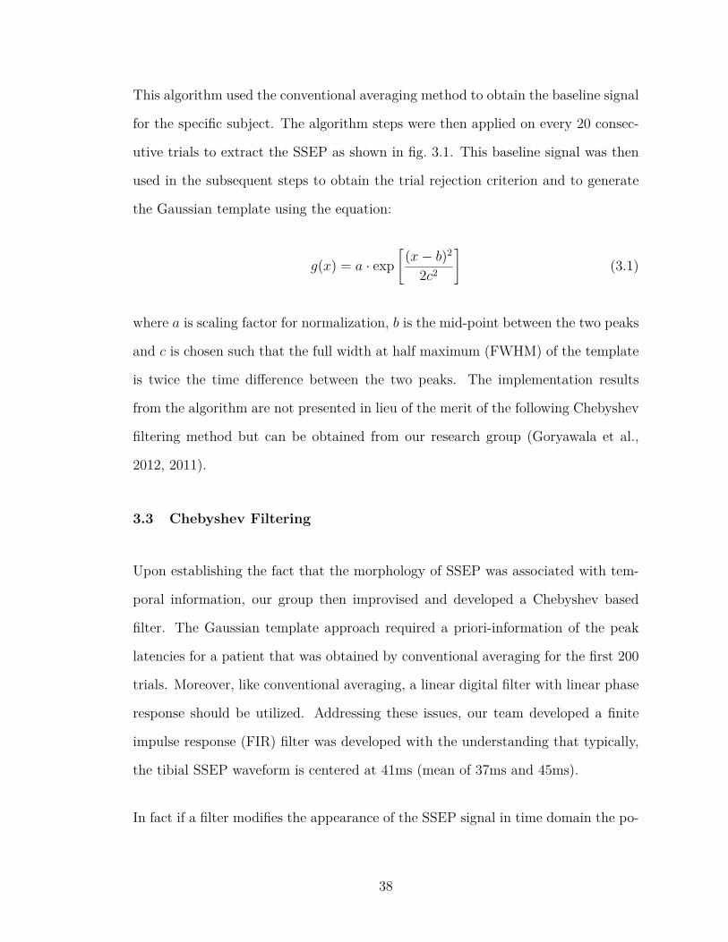
This algorithm used the conventional averaging method to obtain the baseline signal

for the specific subject. The algorithm steps were then applied on every 20 consec-

utive trials to extract the SSEP as shown in fig. 3.1. This baseline signal was then

used in the subsequent steps to obtain the trial rejection criterion and to generate

the Gaussian template using the equation:

g(x) = a · exp[

(x− b)2

2c2

](3.1)

where a is scaling factor for normalization, b is the mid-point between the two peaks

and c is chosen such that the full width at half maximum (FWHM) of the template

is twice the time difference between the two peaks. The implementation results

from the algorithm are not presented in lieu of the merit of the following Chebyshev

filtering method but can be obtained from our research group (Goryawala et al.,

2012, 2011).

3.3 Chebyshev Filtering

Upon establishing the fact that the morphology of SSEP was associated with tem-

poral information, our group then improvised and developed a Chebyshev based

filter. The Gaussian template approach required a priori-information of the peak

latencies for a patient that was obtained by conventional averaging for the first 200

trials. Moreover, like conventional averaging, a linear digital filter with linear phase

response should be utilized. Addressing these issues, our team developed a finite

impulse response (FIR) filter was developed with the understanding that typically,

the tibial SSEP waveform is centered at 41ms (mean of 37ms and 45ms).

In fact if a filter modifies the appearance of the SSEP signal in time domain the po-

38

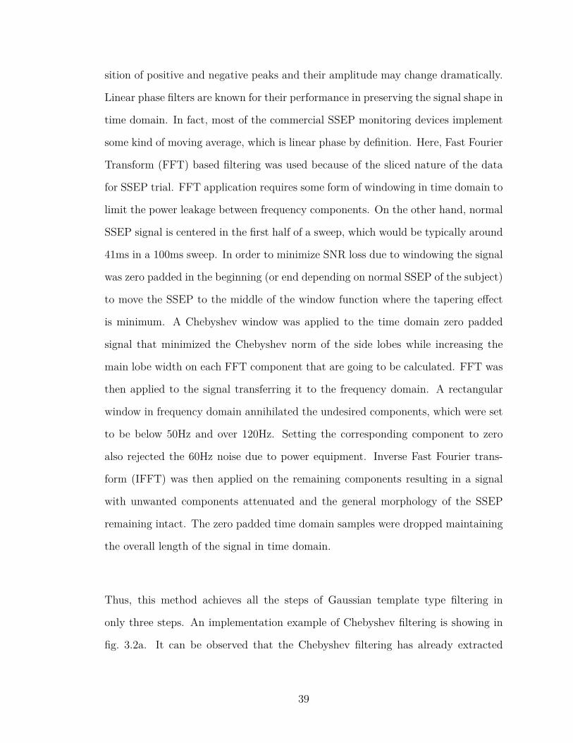
sition of positive and negative peaks and their amplitude may change dramatically.

Linear phase filters are known for their performance in preserving the signal shape in

time domain. In fact, most of the commercial SSEP monitoring devices implement

some kind of moving average, which is linear phase by definition. Here, Fast Fourier

Transform (FFT) based filtering was used because of the sliced nature of the data

for SSEP trial. FFT application requires some form of windowing in time domain to

limit the power leakage between frequency components. On the other hand, normal

SSEP signal is centered in the first half of a sweep, which would be typically around

41ms in a 100ms sweep. In order to minimize SNR loss due to windowing the signal

was zero padded in the beginning (or end depending on normal SSEP of the subject)

to move the SSEP to the middle of the window function where the tapering effect

is minimum. A Chebyshev window was applied to the time domain zero padded

signal that minimized the Chebyshev norm of the side lobes while increasing the

main lobe width on each FFT component that are going to be calculated. FFT was

then applied to the signal transferring it to the frequency domain. A rectangular

window in frequency domain annihilated the undesired components, which were set

to be below 50Hz and over 120Hz. Setting the corresponding component to zero

also rejected the 60Hz noise due to power equipment. Inverse Fast Fourier trans-

form (IFFT) was then applied on the remaining components resulting in a signal

with unwanted components attenuated and the general morphology of the SSEP

remaining intact. The zero padded time domain samples were dropped maintaining

the overall length of the signal in time domain.

Thus, this method achieves all the steps of Gaussian template type filtering in

only three steps. An implementation example of Chebyshev filtering is showing in

fig. 3.2a. It can be observed that the Chebyshev filtering has already extracted

39

the morphology of the SSEP signal from one trial. However, the morphology may

not always be true to the characteristics due to the unpredictable nature of the

background brain activity as shown in fig. 3.2b.

To analyze the effectiveness of the algorithm, we check the SNR for the algorithm

with that of the clinical approach. The formula for calculating the SNR is as follows:

SNR = 20× log10

(SSEP signal amplitude

noise amplitude

)(3.2)

The signal is obtained by taking the ensemble average of all the available trials and

the noise signal is obtained by alternate addition and subtraction of all the available

trials. This method allows us to obtain the SSEP signal and the noise without

the SSEP signal at both the input and output of the algorithm (MacDonald et al.,

2005). Figure 3.3 shows a typical SNR comparison wherein the proposed Chebyshev

filtering provides with an SNR of 6.58dB using just 12 trials as compared with clinical

averaging with takes as many as 114 trials to achieve the same SNR.

40

��

��

��

��

��

��

��

��

Figure 3.1: Outline of the SSEP recording timeline as compared with the clinicalmonitoring. By the time one clinical SSEP is obtained, the algorithm version 2obtained 10 SSEP signals.

0 10 20 30 40 50 60 70 80 90 100

−5

−4

−3

−2

−1

0

1

2

3

4

Time (ms)

Am

plit

ude (

µV

)

Cheby. filtered

Raw

Actual SSEP

(a) Morphology clearly identifiable.

41

0 10 20 30 40 50 60 70 80 90 100

−4

−3

−2

−1

0

1

2

3

Time (ms)

Am

plit

ude (

µV

)

Cheby. filtered

Raw

Actual SSEP

(b) Morphology not so clearly identifiable.

Figure 3.2: Comparison of signals before and after applying Chebyshev filtering withthe actual average signal.

42

50 100 150 200 250 300−15

−10

−5

0

5

10

15

20

25

SNR=6.58 @N=12 SNR=6.651 @N=114

Number of Trials

SN

R (

dB

)

Signal to Noise Ratio (SNR)

Raw SSEP

Time Frequency Filtered SSEP

Figure 3.3: The signal to noise ratio (SNR) comparison for raw signals and after.SNR values are provided for the two cases when 12 trials are used and for 200 rawtrials.

43

CHAPTER 4

ALGORITHM VERSION 3 – COMBINATION OF EIGEN & TEMPORAL

FILTERING

Version 1 of the algorithm involved direct application of the eigen based filtering on

the recorded data and followed by frequency based filtering. In version 2, a frequency

based Gaussian template was used to achieve the same goal. The combination of the

two opens up a wider angle of view to understand better the physiology of SSEP. A

flowchart which summarizes the key steps taken is shown in fig. 4.1.

4.1 Merits of Pre-filtering

Linear phase filters are known for their performance in preserving the signal shape

in the time domain. In fact, most of the commercial SSEP monitoring devices

implement some kind of moving average, which is linear phase by definition. Here,

FFT based filtering was used as explained in the previous chapter.

A Chebyshev window is applied in this case to the time domain zero padded signal

that minimizes the Chebyshev norm of the side lobes while increasing the main lobe

width on each FFT component that are going to be calculated.

4.2 Implementation

4.2.1 Data Acquisition

The data acquisition process in this implementation involved creating a matrix of 12

successive unrejected trials for each bipolar recording channel. The same rejection

44

START

Initialize N trials=1, N reject=0, X=empty

Obtain the most recent sweep= x

Rejection criterion:

max|x|{> 15 OR

= 0

Perform chebychev windowing in time domain.Remove 60Hz and its harmonics.

Append the signal x to the matrix XIncrement N trials by one.

Is N trials = 12?

Perform Eigen-space filtering onmatrix X

SSEP approximation is the time-average of thereconstructed signals.

Perform Walsh-operator convolution to detectthe P37 and N45 peaks.

CONTINUE TILL END OF SURGERY

No(N reject++)

Yes No

Yes

Figure 4.1: Flowchart for the complete algorithm version 3.

45

-6-4-20246A

mplitude

X(1) X(2) X(3)

-6-4-20246

X(4) X(5) X(6)

-6-4-20246

X(7) X(8) X(9)

-6-4-202460 20 40 60 80 100

X(10)

0 20 40 60 80 100

X(11)

0 20 40 60 80 100

Time (ms)

X(12)

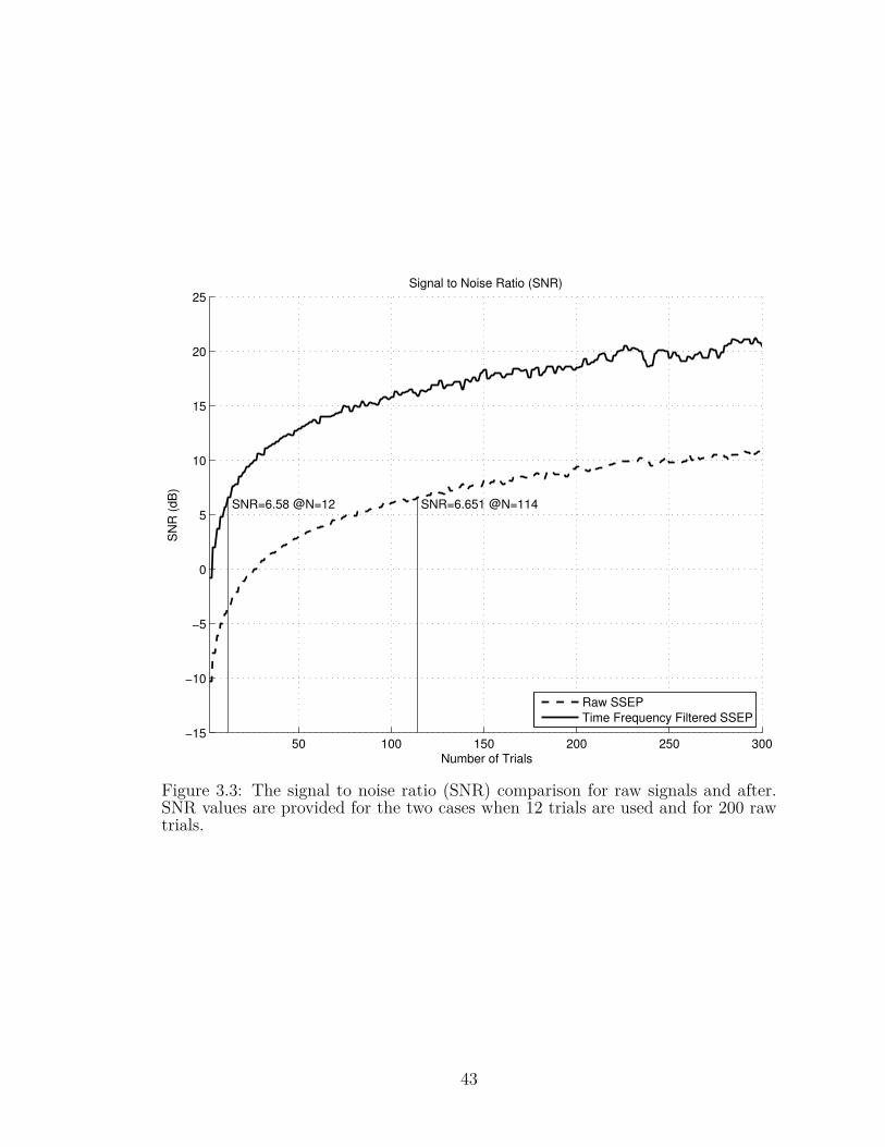
Figure 4.2: A set of twelve successive unrejected recordings for the patient 7 intable 4.1.

46

criterion was used to follow the requirements in the clinical settings i.e., if the

amplitude is 0µV or greater than 25µV, reject the signal from further analysis fig. 4.2.

4.2.2 Pre-filtering or Pre-conditioning

Each of the 12 signals was then preconditioned to remove the 60Hz noise and band

limit the signal from 50Hz to 120Hz. To achieve this with minimum spectral leak-

age, the signal was first zero-padded in time domain and a Chebyshev window was

applied. The signal was then converted to frequency domain using fast Fourier

transform (FFT) (Madhok et al., 2010; Hu et al., 2011b), where the rectangular

window was applied. The inverse FFT will result in a signal devoid of unwanted

frequency components and the zero padding can now be removed to get back a signal

of 100ms.

4.2.3 Eigen Space

A form of principal component analysis used for blind source separation, called

AMUSE was used to analyze the eigen-components of the data set. Experimental

evaluations showed that it was always the first three components that contribute

to the noise and background EEG in the recordings. Eliminating these components

was expected to result in the SSEP from that recording. Figure 4.3 shows the signals

before pre-filtering and fig. 4.4 shows the signals after performing the pre-filtering

operation.

47

Table4.1:

Details

ofthepa

tientswith

age,

sex,

thesurgical

procedurethey

underw

ent,

thetim

epe

riodof

thesurgery

durin

gwhich

theSS

EPwe

rerecorded,the

numbe

roftria

lsused

pera

ssessm

entfor

clinical

mon

itorin

gby

signa

l-averaging

metho

d,theaccuracy

oftheprop

osed

algorit

hman

dthelast

columnshow

sthestan

dard

deviationof

thepe

aklatencies

from

theba

selin

evalues.

Patie

nt#

Sex

(M/F

)Age

Surgical

Procedure

Duration

(hrs)

No.

oftrials

per

assess-

ment

Accuracy

Stan

dard

Devia-

tion

(σ)

1F

41Cerebrala

neurysm

clipping

2200

92.7%

3.0m

s2

F47

T10-S1po

steriorspinal

fusio

n2

200

88.1%

3.2m

s3

F71

Cerebrala

neurysm

clipping

2200

95.9%

1.7m

s4

F75

T10-S1po

steriorspinal

fusio

n6

200

94.4%

1.9m

s5

M73

Anterioran

dpo

steriorlumba

rfusio

n4

3294.7%

1.9m

s6

F66

T4-S1

posteriorspinal

fusio

n1.5

138

91.2%

2.1m

s7

F11

Posteriorspinal

fusio

nforscoliosis

2113

89.4%

2.1m

s8

F64

L5-S1TLIF

2213

96.3%

1.5m

s9

F76

T10-S1po

steriorspinal

fusio

n2.5

200

87.2%

3.6m

s10

F21

T2-T12

post

spinal

fusio

n3.5

200

95.4%

1.2m

s11

M70

Carotid

enda

rectom

y1.4

200

94.3%

1.8m

s12

F58

AVfistula

1.2

200

78.6%

4.2m

s

48

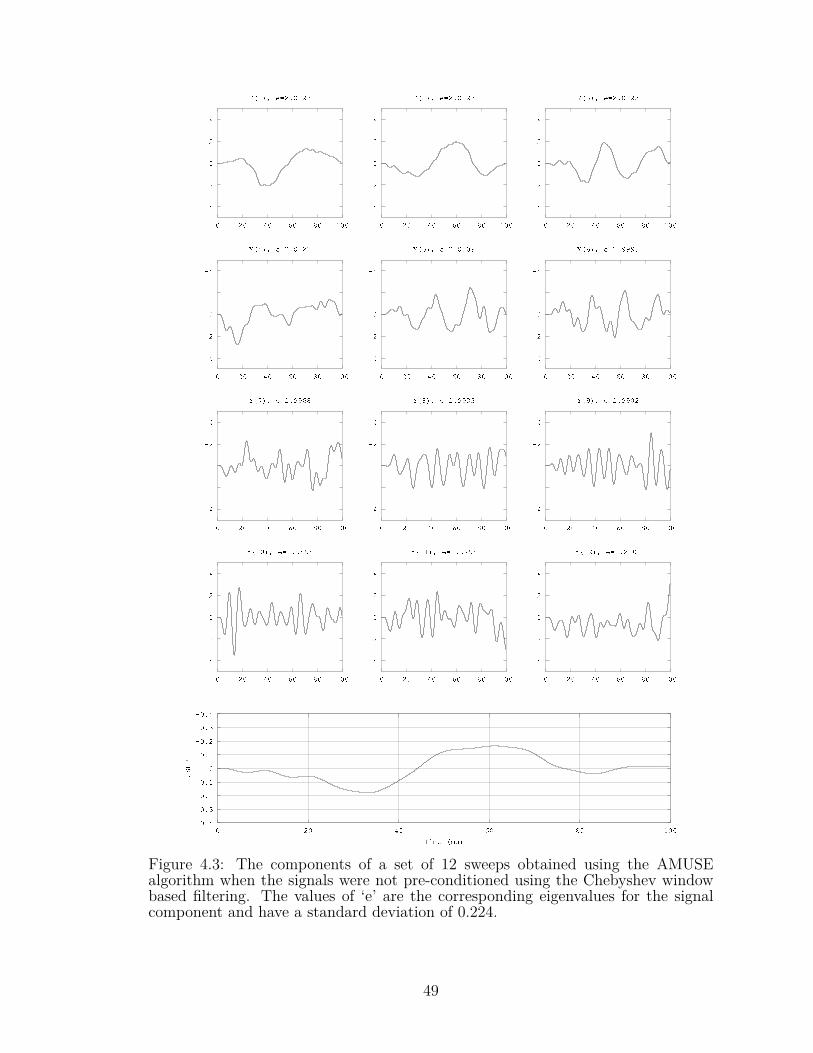
Figure 4.3: The components of a set of 12 sweeps obtained using the AMUSEalgorithm when the signals were not pre-conditioned using the Chebyshev windowbased filtering. The values of ‘e’ are the corresponding eigenvalues for the signalcomponent and have a standard deviation of 0.224.

49

Figure 4.4: The components of a set of 12 sweeps obtained using the AMUSEalgorithm when the signals were pre-conditioned using the Chebyshev window basedfiltering. The values of ‘e’ for each component are the corresponding eigenvalues andhave a standard deviation of 0.0034.

50

4.2.4 Reconstruction

These filtered components are used to reconstruct the signals Xr fig. 4.5 that was

the SSEP signal from each of the recordings. These 12 reconstructed signals are

then averaged in time and the time-locked SSEP signal was obtained.

4.2.5 Information Extraction

A Walsh kernel representing the first derivative can then be used to automate the

peak detection (Adjouadi et al., 2004) and was used on the extracted SSEP signal

to obtain the P37 and N45 peak latencies and the peak-to-peak amplitude fig. 4.6.

4.3 Results

The algorithm in this version was robust enough that it would run continuously

receiving the EEG recordings, checking for corrupt signals and processing a set

of 12 successive good trials to provide with a morphologically and mathematically

accurate SSEP waveform. The timeline for the algorithm is represented in fig. 4.7.

4.3.1 Implementation

This new algorithm provides an improvement in preserving the morphological char-

acteristics of the SSEP waveforms from earlier versions 1 and 2. The previous algo-

rithm addressed the issue of automated peak detection and presented an algorithm

that was designed for the specific intension of being able to verify the waveform by

manual inspection. In this new algorithm the objective was to extract automati-

cally the SSEP with a minimum number of sweeps or trials and yet obtain the same

51

Figure 4.5: A comparison of the components and the extracted SSEP from fig. 4.3(dotted lines) and fig. 4.4 (solid lines).

52

-0.64

0.0

0.5-0.7

0.0

0.50 20 40 60 80 100

Time (ms)

AlgorithmAveragingP37 N45

Figure 4.6: Comparison of SSEP extracted by the algorithm using only 12 trialswith that obtained using the traditional method of averaging of 113 trials.

morphology as that obtained with the maximum number of trials traditionally used.

Significant comfort is reached when time latencies and morphology conform to the

true signal.

To weigh the merits of the proposed algorithm, and for illustrative purposes, imple-

mentation steps performed on the data for patient number 8 in table 4.1 throughout

the 2-hour surgical procedure with all the 479 extracted SSEP waveforms is pre-

sented in fig. 4.8. Figure 4.8 displays the extracted waveforms through another

similar surgery of patient 7. The baseline signal is the very first extracted SSEP

using the same procedure on the first 12 sweeps and is at the very top of the fig-

53

ure. The detected P37 and N45 latencies have been marked with vertical lines for

reference. All the 12 tested surgical outcomes were clinically successful without

any alarms raised during the surgeries and no neurological damage to the patients

were found. To analyze the effectiveness of the algorithm, we check the SNR for

the algorithm with that of the clinical approach. The formula used for calculating

the SNR was presented warlier in eq. (3.2). The signal is obtained by taking the

ensemble average of all the available trials and the noise signal is obtained by alter-

nate addition and subtraction of all the available trials. This method allows us to

obtain the SSEP signal and the noise without the SSEP signal at both the input

and output of the algorithm (MacDonald et al., 2005). Figure 4.9 shows the SNR

improvement achieved by application of the Chebyshev time-frequency windowing

method. Table 4.2 summarizes the results from the implementation of the algorithm

on all 12 patients.

4.3.2 False Alarms

The sensitivity and accuracy of the algorithm can be analyzed based on the number

of detections by the algorithm and the actual alarms raised. In the surgeries per-

formed, however, although there were no alarms raised but the proposed algorithm

��

��

��

��

��

��

��

��

Figure 4.7: Outline of the SSEP recording timeline as compared with the clinicalmonitoring. By the time one clinical SSEP is obtained, the algorithm version 3obtaining 12 SSEP signals.

54

(a) Sequence of 479 SSEPs of 100ms extracted in sequence during the two hour-longsurgery of patient# 7 in table 4.1 from the C3–C4 channel. The baseline signal (earliestSSEP) is on the very top and the last SSEP extracted is at the bottom. Two verticallines mark the P37 (first one on the left at 41ms) and N45 (second vertical line at 48.5ms)baseline values for reference. Five of the signals in the region marked by a box are displayedin the adjacent plot for illustration. The numbers marked on them are the set numbersfrom which the SSEP were extracted.

55

(b) Sequence of 358 SSEPs of 100ms extracted in sequence during the two hour-longsurgery of patient# 8 in table 4.1 from the C3–C4 channel. The baseline signal (earliestSSEP) is on the very top and the last SSEP extracted is at the bottom. Two vertical linesmark the P37 (first one on the left at 39.3ms) and N45 (second vertical line at 46.3ms)baseline values for reference.

Figure 4.8: Sequence of extracted SSEPs of 100ms throughout the surgery.

56

Table 4.2: Summary of the results from the implementation of the proposed algo-rithm showing the average variability in the time latency and amplitude and thetotal number of false alarms raised for each patient.

Patient# Average variability (%) Number offalse alarmsTime latency Amplitude

1 5.1 8 42 3.2 29 33 1.3 22 44 5.8 18 55 2.6 13 46 1.9 12 27 2.3 20 28 7.1 26 59 3.6 19 410 4.1 25 311 2.9 18 312 2.4 15 2

Average: 3.3 19 1.6 /hr

did raise alarms that can be considered as false alarms. The false alarms detected

were due to peak-to-peak amplitude variation of more than 50%, fig. 4.10. It was

shown in table 4.2 that there were, on an average, 1.6 false alarms per hour. If

the false alarms are quantized as the percentage of false alarms occurring per sub-

ject for every set of 12 trials used to extract the SSEP, we obtain an average of

0.09% of false alarms for this specific presented study. It must be noted that the

extracted SSEP signals are obtained every twelve trials and hence the short-term

SSEP changes that go unnoticed by the conventional averaging method are easily

acquired using the algorithm. Hence, for a true positive, the changes must persist

for 12 successive SSEP extracted using the algorithm. No such case was observed

in the study confirming that no alarms were raised during the procedures.

As an example, the implementation results for patient 10 from table 4.1 are pre-

sented in table 4.3. Another example of consistency through a surgical procedure is

57

displayed in fig. 4.11.

58

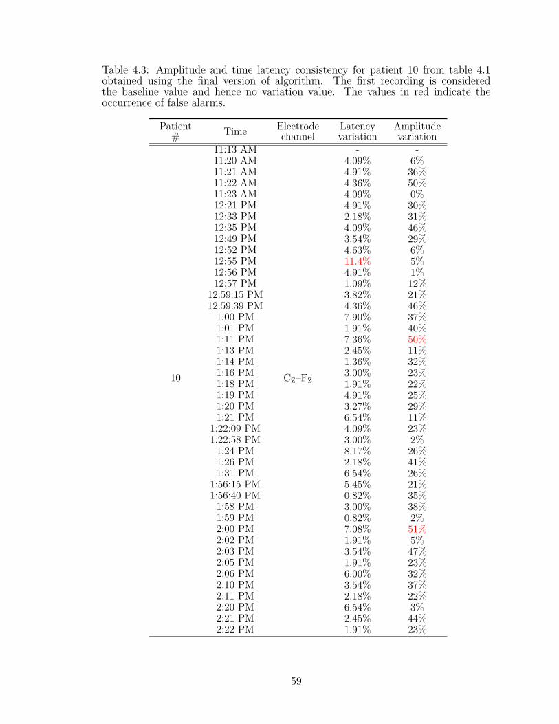
Table 4.3: Amplitude and time latency consistency for patient 10 from table 4.1obtained using the final version of algorithm. The first recording is consideredthe baseline value and hence no variation value. The values in red indicate theoccurrence of false alarms.

Patient# Time Electrode

channelLatencyvariation

Amplitudevariation

10

11:13 AM

CZ–FZ

- -11:20 AM 4.09% 6%11:21 AM 4.91% 36%11:22 AM 4.36% 50%11:23 AM 4.09% 0%12:21 PM 4.91% 30%12:33 PM 2.18% 31%12:35 PM 4.09% 46%12:49 PM 3.54% 29%12:52 PM 4.63% 6%12:55 PM 11.4% 5%12:56 PM 4.91% 1%12:57 PM 1.09% 12%

12:59:15 PM 3.82% 21%12:59:39 PM 4.36% 46%1:00 PM 7.90% 37%1:01 PM 1.91% 40%1:11 PM 7.36% 50%1:13 PM 2.45% 11%1:14 PM 1.36% 32%1:16 PM 3.00% 23%1:18 PM 1.91% 22%1:19 PM 4.91% 25%1:20 PM 3.27% 29%1:21 PM 6.54% 11%

1:22:09 PM 4.09% 23%1:22:58 PM 3.00% 2%1:24 PM 8.17% 26%1:26 PM 2.18% 41%1:31 PM 6.54% 26%

1:56:15 PM 5.45% 21%1:56:40 PM 0.82% 35%1:58 PM 3.00% 38%1:59 PM 0.82% 2%2:00 PM 7.08% 51%2:02 PM 1.91% 5%2:03 PM 3.54% 47%2:05 PM 1.91% 23%2:06 PM 6.00% 32%2:10 PM 3.54% 37%2:11 PM 2.18% 22%2:20 PM 6.54% 3%2:21 PM 2.45% 44%2:22 PM 1.91% 23%

59

0

5

10

15

20

25

30

50 100 150 200 250 300

SNR (dB)

Number of trials

RawPreconditioned

SNR=9.2907

SNR=4.7834

SNR=1.2935

N=12

Figure 4.9: The signal to noise ratio (SNR) comparison for clinical SSEP signalsand post-processed signals. SNR values are provided for the two cases when 12 trialsare used and for 200 raw trials.

60

-0.8

-0.6

-0.4

-0.2

0

0.2

0.4

0.6

0.80 20 40 60 80 100

SSEP Amplitude (mV)

Time (ms)

BaselineFalse Positive

Figure 4.10: Comparison of a false positive SSEP signals as detected due to highamplitude variation for patient 8 in table 4.1 C3–C4 montage at 23min through theprocedure with the baseline SSEP.

61

0

0

0

0

0

0 20 40 60 80 100

Time (ms)

Baseline

37min

1hr 14min

1hr 51min

2hr 28min

0.3µV

P37 N45

Figure 4.11: The baseline signal and tSSEP signals at different times shown forcomparison. The vertical markers are for average P37 and N45 peak latencies forPatient# 9 from table 4.1. Note that the vertical axis is inverted, with positivedirection going downward following the convention of displaying SSEP.

62

CHAPTER 5

CONCLUSIONS AND FUTURE WORK

The new algorithms developed and presented in the dissertation attempted to ad-

dress the hypotheses proposed and questions raised in this study. The primary

objective was to understand the characteristics of an SSEP and classify it from

background brain activity, a task that is critical in monitoring spinal surgeries.

5.1 Conclusions from algorithm versions

5.1.1 Version 1

The eigen-decomposition process helped reduce significantly the number of trials, a

clinical outcome that is highly desirable, and allowed for a thorough assessment that

delineated signal trend from noise. The use of the Walsh operator proved highly

effective in detecting the evoked potential peak latencies using an optimal number

of trials (in this study, limited to 10). The algorithm no longer depends on the

signal morphology and automates the process from selection of a minimum number

of trials based on their frequency response, applying the algorithm on them and

using the unique Walsh transformation method to automatically indicate the SSEP

response and the peak latencies. The results from the automated detection scheme

and interpretation of the characteristic peak using the Walsh operation coincide

with expertsâĂŹ opinions.

For all of the cases the noted average misalignment between the clinical peak la-

tencies and those obtained using the proposed algorithm, including both bipolar

channels, was 3.38ms and 4.3ms for P37 and N45, respectively. It should be stated

that when such misalignments happen during a surgical procedure, even when a

63

maximum number of trials is used, clinicians select one of the two channels that is

viewed as more representative of the SSEP morphology.

The Walsh operator proved highly effective in identifying the SSEP occurrence even

when the morphology of the signal is quite different from that obtained at a much

higher number of trials. In the automated process, a thorough analysis yielded a

better mathematical assessment of the noise signal involved in evoked potentials.

Since there are no intensive mathematical operations involved in the algorithm, it

can be feasibly realized in hardware form and/or integrated in the present systems

to establish a very valuable tool in IONM.

5.1.2 Version 2

Consistency in the results is also satisfied by the current algorithm for SSEP de-

tection, which demonstrated an average percentage deviation of 4.47 ± 3.33% and

3.73 ± 3.92% in the detection of the time latencies of the P37 and N45 peaks, re-

spectively, using the C3–C4 channel; and 4.60 ± 4.18% and 3.30 ± 2.46% when the

CZ–FZ channel is used. Also, the algorithm was able to get consistent results in the

detection of the peak-to-peak amplitude of the SSEP signals. The algorithm demon-

strated an average percentage deviation of 19.81±13.84% and 23.97±24.23% in the

calculation of the SSEP peak-to-peak amplitude for the C3–C4 and CZ–FZ channels,

respectively. These values are below the clinically approved levels for deviation of

10% for the time latencies and 50% for the peak-to-peak amplitude. What is even

more important is the fact that the results were found to be consistent throughout

the surgical procedure for all the patients considered.

During surgery, the decisions are based on either one of the channels: C3–C4 and

64

Table 5.1: Summary of results showing the average percentage error and percentagedeviation in SSEP detection using either C3–C4 channel or CZ–FZ channels. Thelogical OR function of the two channels is denoted by symbol (V).

Electrode % Error % Deviation from baselineP37 N45 P37 N45 p-p Amp

C3–C4 3.70± 3.04 4.03± 3.28 4.47± 3.33 3.73± 3.92 19.81± 13.84CZ–FZ 3.51± 3.68 4.07± 3.35 4.60± 4.18 3.30± 2.46 23.97± 24.23

(C3–C4) V(CZ–FZ) 1.91± 1.38 2.11± 1.82 2.46± 1.84 1.88± 1.26 11.14± 10.44

CZ–FZ. The clinicians select one of the two channels that is viewed as more represen-

tative of the SSEP morphology. Taking this into consideration, table 5.1 presents

the results of a logical ‘OR’ function that represents the results obtained by us-

ing the results from the electrode that provided the better results. Table 5.1 thus

provides an estimate of the best-case scenario where the electrode that provided a

better detection of the SSEP is picked for the analysis. Please note that patient

4 was not included in the analysis for this OR function analysis since the C3–C4

data were not available. The results in table 5.1 demonstrate that the algorithm is

capable of detecting the P37 and N45 peak latencies with a very high accuracy of

about 98% in situations when the best electrode channel is chosen. As such, the

average percentage deviations from the baseline are also reduced by approximately

a factor of 2.

Various other techniques have addressed the problem of SSEP detection with the aim

of reducing the number of trails. It was shown that 50 input trials can provide similar

performance as compared to the ones obtained using 1000 trials (Lam et al., 2005).

Single trial determination of SSEP using a combination of EEG-based probabilistic

independent component analysis and wavelet filtering had been presented (Hu et al.,

2011b). Another study had also shown the determination of SSEPs using 80 trials

which provided an average accuracy of 0.75% ± 1.12 and 0.86% ± 0.37 of the P37

65

and N45 peaks (Hu et al., 2009). Liu et al. presented an independent component

analysis (ICA) method for the detection of SSEP monitoring using 300 simulated

trials (Liu et al., 2007).

The developed algorithm provides a simple yet precise solution toward the detection

of the SSEP waveform from a significantly reduced number of trials. Instructive

steps were consolidated from empirical evaluations and observations to ensure that

noisy signals were removed using key pre-processing steps. These included (1) a

statistical threshold on the amplitude of the signals which removed a priori any

trial whose change is one standard deviation higher than the mean of the standard

deviations of all 30 channels; and on the remaining trials, (2) the use of a fouth-order

Butterworth notch filter with a stop band from 55 Hz to 65 Hz that removed the

ubiquitous 60 Hz noise; (3) the use of a fifth-order Butterworth low-pass filter with a

cut-off frequency of 300 Hz that served as a notch filter to remove any unwarranted

high-frequency components, which in the context of the desired SSEP signal are

considered as noise; and (4) the use of a moving average filter with a 25-point

window that served as a smoothing filter.

With all these initial preprocessing steps properly executed, a significant contri-

bution of this algorithm is in introducing patient-specific Gaussian templates that

envelop the SSEPs, delineating them clearly from other portions of the signal and

any remnant artifacts embedded within a given trial.

5.1.3 Version 3

The algorithm is able to exploit multiple characteristics of the SSEP simultaneously

viz., the morphology of the signal in time domain, the frequency characteristics and

66

the eigen space components that contribute to the signal. The AMUSE algorithm

is able to separate the SSEP with the background brain activity but is not able to

preserve the signal morphology in the time domain.

The novelty of the approach was the use of Chebyshev windowing for precondi-

tioning the signal before linear filtering for 60Hz notch and low pass filter. The

windowing method considerably improved the SNR of the raw signals (fig. 4.9) but

still required 50 or more number of trials to obtain the SNR close to practical values

(Goryawala et al., 2012; Hu et al., 2003). Thus enhancing the prospects for the

AMUSE algorithm to better classify the signal components. The preconditioning

improved the SNR by about 4dB in the first twelve trials. The important contribu-

tion was the improvement in SNR by preconditioning in a much reduced number of

trials and coupled with the AMUSE algorithm to better extract the SSEP preserving

the morphology of the signal.

When linear filtering was performed without this pre-conditioning, the signal com-

ponents obtained in the AMUSE algorithm did not show a trend in the signal-noise

power characteristics and the standard deviation of the eigenvalues was high, typ-

ically of the order of 0.12. Though the extracted SSEP was clearly identifiable

(fig. 4.3), the signal showed spreading in time and was reconstructed from the com-

ponents with the higher eigenvalues. With the windowing, however, as was illus-

trated in fig. 4.4, the eigenvalues were more organized with noise power concentrated

in the components with the higher eigenvalues. This is because the Chebyshev win-

dow limits the spectral power leakage and concentrates them in the frequency band

of interest thus improving the contrast of the signal. Figures 4.3 and 4.4 depicted

the same set of 12 sweeps that form the 5th SSEP of the fig. 4.8, the former without

the Chebyshev windowing and the latter with Chebyshev windowing. These two

67

results were superimposed and displayed in fig. 4.6 for comparative purposes.

The AMUSE algorithm performed in the same manner in both cases and was able

to separate the signal components attributing to the background EEG. However,

with no signal preconditioning, the signal components showed (1) wide variation

with respect to their corresponding eigenvalues and (2) wide amplitude variations;

whereas with conditioning, the components showed (1) close and evenly distributed

eigenvalues and (2) the signal power of the components was relatively uniform.

It was also interesting to observe that the signal components with and without the

preconditioning showed regions of very high correlation. The signal preconditioning

thus helped to improve the contrast between the signal components that the AMUSE

algorithm extracts. These results provide the impetus to proceed with an exhaustive

number of implementations for further confirmation.

The algorithm was tested on 12 patients and the results were presented in table 4.2.

The algorithm was successful in extracting the SSEP signals throughout all surgeries.

These results were obtained using only 12 trials that passed the exclusion criterion

and checks for the consistencies and any causes for false alarms. The 12 surgical

cases did not have any alarms raised during the clinical procedures. The algorithm,

however, did raise alarms and these were termed as ‘false alarms’. This fact assures

us that the algorithm is capable of detecting and raising alarms. As such, the

accuracy of the algorithm was defined as

%Accuracy =(

1− no.of false alarmsno.of SSEP signals

)× 100 (5.1)

The sensitivity and accuracy of the algorithm can be analyzed based on the number

68

of detections by the algorithm and the actual alarms raised. In the surgeries that

were performed, no alarms were raised throughout; however the algorithm did raise

alarms that were considered as false alarms. It was shown in table 4.2 that there

are, on an average, 1.6 false alarms per hour. If the false alarms are quantized as

the percentage of false alarms occurring per subject for every set of 12 trials used

to extract the SSEP, we obtain an average of 0.09% of false alarms.

It is very important to note that since the extracted SSEP signals are obtained every

twelve trials and hence the short-term SSEP changes that would have otherwise gone

unnoticed by the conventional averaging method are easily detected when using the

proposed algorithm. Hence, for a true positive, the changes must persist for 12

successive SSEP signals extracted using the algorithm. No such case was observed

in the study confirming that no alarms were raised during the procedures.

On an average, the algorithm raised 1.6 false alarms per hour and presented an

accuracy of 91.5%. An example of a typical SSEP extracted using the proposed

algorithm for a given subject at five different instances of time during the surgery

was shown in fig. 4.10. Note the merits of using Chebyshev as means to preserve

the morphology of the SSEP signal.

5.2 Discussion

In version 1, it was observed that even though the automation scheme was shown to

be viable, the IIR filtering applied at the very end might not give an SSEP true to

its morphological characteristics to be observed by experienced eye (Vedala et al.,

2012b). We observed, in the final version 3, that such filtering is more beneficial

when applied prior to eigen-space filtering. Conventional systems also adopt a sim-

69

ilar approach of filtering using moving average type filters after signal averaging.

These are linear phase filters. Hence, we choose Chebyshev time windowing prior

to eigen-space filtering. This has the merit of limiting power leakage of the fre-

quency components of SSEP to adjacent frequencies. A rectangular window in the

frequency domain eliminated undesired frequency components and preserved those

frequencies that contribute most to the SSEP signal. It is also effective in removing

the 60Hz noise introduced by the electrical equipment in the vicinity.

It is a long known fact that EEG sources are non-stationary (Delorme et al., 2012),

however, during the 100ms time windows, as is common in IONM, the EEG sources

are considered quasi-stationary (Kaplan et al., 2005; Zygierewicz et al., 2006), and

hence the AMUSE algorithm was able to identify only the known stationary SSEP

component. On the other hand, the use of Chebyshev time window a priori made

certain that any other stationary and quasi-stationary components are eliminated.

The current algorithms assume that the SSEP does not change during the time

when the 200 or more trials are recorded and rely on the frequency characteristics

of the signal rather than the SSEP morphology in time domain. Other proposed

approaches also tend to focus on only one aspect of the SSEP characteristics, mainly

in the frequency domain. The present approach in retrospect focuses on preserving

the time domain features of SSEP and eliminates the inter-trial variance and extracts

the SSEP while considering the ongoing brain activity.

To ascertain the validity of the algorithm, we present the results of the implementa-

tion of the algorithm on 12 surgical procedures that lasted anywhere between 1.5 and

6hrs. These surgeries were successful with no resulting neurophysiological effects.

The algorithm also ascertained that the peak latencies and peak-to-peak amplitudes

70

are within the required limits to prove consistency. The algorithm, however, raised

1.6 false alarms per hour. This can be considered as a good sign because this proves

that the algorithm is capable of detecting a true alarm, although not experienced

in these surgeries.

5.3 Future Study and Recommendations

5.3.1 Exhaustive study

The data available for the study contained no true positive cases and hence, a critical

study involving sensitivity of the algorithm could not be presented. Future study

should involve the following:

(a) Implementation of algorithm on patients where a true clinical alarm was indeed

raised in order to assess the algorithm’s accuracy and sensitivity in detecting

true positives.

(b) Implementation of algorithm on SSEP waveforms from other extremities (e.g.

ulnar nerve).

(c) Implementation of algorithm on expanded subject cases involving appropriate

statistics that include gender, height, type of surgical procedure and the type

of anaesthesia used.

5.3.2 Practical implementation

The simplistic nature of the final algorithm (version 3) makes it possible for its

potential implementation in both hardware and software forms. The present IONM

software systems can readily incorporate the algorithm and provide the benefits

71

readily. The hardware implementation provides many advantages. Primarily, im-

plementation in hardware form would minimize both the setup process and the

processing requirements in the operating theater, but at the same time providing

with the same benefits of a software based system.

72

REFERENCES

Adjouadi, M., Cabrerizo, M., Ayala, M., Sanchez, D., Yaylali, I., Jayakar, P., andBarreto, A. (2005). Detection of interictal spikes and artifactual data through or-thogonal transformations. Journal of clinical neurophysiology : official publicationof the American Electroencephalographic Society, 22(1):53–64.

Adjouadi, M. and Candocia, F. (1994). A stereo matching paradigm based onthe Walsh transformation. IEEE Transactions on Pattern Analysis and MachineIntelligence, 16(12):1212–1218.

Adjouadi, M., Candocia, F., and Riley, J. (1996). Exploiting Walsh-based attributesto stereo vision. IEEE Transactions on Signal Processing, 44(2):409–420.

Adjouadi, M., Sanchez, D., Cabrerizo, M., Ayala, M., Jayakar, P., Yaylali, I., andBarreto, A. (2004). Interictal spike detection using the Walsh transform. IEEEtransactions on bio-medical engineering, 51(5):868–72.

Bai, O., Nakamura, M., Nagamine, T., and Shibasaki, H. (2001). Parametric mod-eling of somatosensory evoked potentials using discrete cosine transform. IEEETransactions on Biomedical Engineering, 48(11):1347–51.

Candocia, F. and Adjouadi, M. (1997). A similarity measure for stereo featurematching. IEEE Transactions on Image Processing, 6(10):1460–4.

Celesia, G. G. (1979). Somatosensory evoked potentials recorded directly from hu-man thalamus and Sm I cortical area. Archives of neurology, 36(7):399–405.

Cichocki, A., Shishkin, S. L., Musha, T., Leonowicz, Z., Asada, T., and Kurachi, T.(2005). EEG filtering based on blind source separation (BSS) for early detection ofAlzheimer’s disease. Clinical neurophysiology : official journal of the InternationalFederation of Clinical Neurophysiology, 116(3):729–37.

Crespo-Garcia, M., Atienza, M., and Cantero, J. L. (2008). Muscle artifact removalfrom human sleep EEG by using independent component analysis. Annals ofBiomedical Engineering, 36(3):467–75.

Crittenden, M. D. (2001). Intraoperative metabolic monitoring of the heart: I. Clin-ical assessment of coronary sinus metabolites. The Annals of Thoracic Surgery,72(6):S2220–S2226.

73

Dawson, G. D. (1947). Cerebral Responses to Electrical Stimulation of PeripheralNerve in Man. Journal of neurology, neurosurgery, and psychiatry, 10(3):134–40.

Deletis, V. (2007). Basic methodological principles of multimodal intraoperativemonitoring during spine surgeries. European spine journal : official publicationof the European Spine Society, the European Spinal Deformity Society, and theEuropean Section of the Cervical Spine Research Society, 16 Suppl 2:S147–52.

Deletis, V. and Sala, F. (2008). Intraoperative neurophysiological monitoring ofthe spinal cord during spinal cord and spine surgery: a review focus on the cor-ticospinal tracts. Clinical neurophysiology : official journal of the InternationalFederation of Clinical Neurophysiology, 119(2):248–64.

Delorme, A., Palmer, J., Onton, J., Oostenveld, R., and Makeig, S. (2012). Inde-pendent EEG sources are dipolar. PloS one, 7(2):e30135.

Dinner, D. S., Lüders, H., Lesser, R. P., Morris, H. H., Barnett, G., and Klem, G.(1986). Intraoperative spinal somatosensory evoked potential monitoring. Journalof neurosurgery, 65(6):807–14.

Epstein, N. E., Danto, J., and Nardi, D. (1993). Evaluation of IntraoperativeSomatosensory-Evoked Potential Monitoring During 100 Cervical Operations.Spine, 18(6):737–747.

Friedman, W. A., Chadwick, G. M., Verhoeven, F. J., Mahla, M., and Day, A. L.(1991). Monitoring of somatosensory evoked potentials during surgery for middlecerebral artery aneurysms. Neurosurgery, 29(1):83–8.

Frigo, M. and Johnson, S. G. S. S. (1998). FFTW: an adaptive software architecturefor the FFT. In Proceedings of the 1998 IEEE International Conference on Acous-tics, Speech and Signal Processing, ICASSP ’98 (Cat. No.98CH36181), volume 3,pages 1381–1384. IEEE.

Fukuda, H., Sonoo, M., and Ishibashi, M. (2007). Muscle afferent contributions totibial nerve somatosensory evoked potentials investigated using knee stimulations.Clinical Neurophysiology, 118(9):2104–2111.

Glaser, E. and Ruchkin, D. S. (1976). Principles of Neurobiological Signal Analysis.Academic Press, New York.

Goryawala, M., Yaylali, I., Cabrerizo, M., Vedala, K., and Adjouadi, M. (2011). Aneffective novel patient specific Gaussian template based scheme for somatosensory

74

evoked potential detection. In 2011 IEEE Signal Processing in Medicine andBiology Symposium (SPMB), pages 1–6, New York, NY. IEEE.

Goryawala, M., Yaylali, I., Cabrerizo, M., Vedala, K., and Adjouadi, M. (2012).An effective intra-operative neurophysiological monitoring scheme for aneurysmclipping and spinal fusion surgeries. Journal of neural engineering, 9(2):026021.

Grundy, B. L. (1983). Intraoperative monitoring of sensory-evoked potentials. Anes-thesiology, 58(1):72–87.

Hargadine, J. R. and Snyder, E. (1982). Brain stem and somatosensory evokedpotentials: application in the operating room and intensive care unit. Bulletin ofthe Los Angeles neurological societies, 47:62–75.

Hu, Y., Liu, H., and Luk, K. D. (2011a). Time-frequency analysis of somatosensoryevoked potentials for intraoperative spinal cord monitoring. Journal of clinicalneurophysiology : official publication of the American Electroencephalographic So-ciety, 28(5):504–11.

Hu, Y., Liu, H., and Luk, K. D. (2011b). Time-frequency analysis of somatosensoryevoked potentials for intraoperative spinal cord monitoring. Journal of clinicalneurophysiology : official publication of the American Electroencephalographic So-ciety, 28(5):504–11.

Hu, Y., Luk, K. D., and Xie, X. (2009). Surface somatosensory evoked poten-tial detection by FPGA based multi-adaptive filter. In 2009 4th InternationalIEEE/EMBS Conference on Neural Engineering, pages 673–676. IEEE.

Hu, Y., Luk, K. D. K., Lu, W. W., and Leong, J. C. Y. (2003). Application of time-frequency analysis to somatosensory evoked potential for intraoperative spinalcord monitoring. Journal of neurology, neurosurgery, and psychiatry, 74(1):82–7.

Hussain, A. M. (2008). A Practical Approach to Neurophysiologic IntraoperativeMonitoring. Demos Medical Publishing.

Jones, S. J., Edgar, M. A., Ransford, A. O., and Thomas, N. P. (1983). A systemfor the electrophysiological monitoring of the spinal cord during operations forscoliosis. The Journal of bone and joint surgery. British volume, 65(2):134–9.

Jou, I.-M., Hsu, C.-C., Chern, T.-C., Chen, W.-Y., and Dau, Y.-C. (2003). Spinalsomatosensory evoked potential evaluation of acute nerve-root injury associatedwith pedicle-screw placement procedures: an experimental study. Journal of

75

orthopaedic research : official publication of the Orthopaedic Research Society,21(2):365–72.

Kany, C. and Treede, R. D. (1997). Median and tibial nerve somatosensory evokedpotentials: middle-latency components from the vicinity of the secondary so-matosensory cortex in humans. Electroencephalography and Clinical Neurophysi-ology, 104(5):402–10.

Kaplan, A. Y., Fingelkurts, A. a., Fingelkurts, A. a., Borisov, S. V., and Dark-hovsky, B. S. (2005). Nonstationary nature of the brain activity as revealed byEEG/MEG: Methodological, practical and conceptual challenges. Signal Process-ing, 85(11):2190–2212.

Khan, M. H., Smith, P. N., Balzer, J. R., Crammond, D., Welch, W. C., Gerszten,P., Sclabassi, R. J., Kang, J. D., and Donaldson, W. F. (2006). Intraopera-tive somatosensory evoked potential monitoring during cervical spine corpectomysurgery: experience with 508 cases. Spine, 31(4):E105–13.

Kilpatrick, C. C., Puig, C., Chohan, L., Monga, M., and Orejuela, F. J. (2010). In-traoperative fetal heart rate monitoring during nonobstetric surgery in pregnancy:a practice survey. Southern medical journal, 103(3):212–5.

Kong, X. and Oiu, T. (2001). Latency change estimation for evoked potentials:A comparison of algorithms. Medical & Biological Engineering & Computing,39(2):208–224.

Lam, A. M., Manninen, P. H., Ferguson, G. G., and Nantau, W. (1991). Monitor-ing electrophysiologic function during carotid endarterectomy: a comparison ofsomatosensory evoked potentials and conventional electroencephalogram. Anes-thesiology, 75(1):15–21.

Lam, B. S. C., Hu, Y., Lu, W. W., Luk, K. D. K., Chang, C. Q., Qiu, W., and Chan,F. H. Y. (2005). Multi-adaptive filtering technique for surface somatosensoryevoked potentials processing. Medical engineering & physics, 27(3):257–66.

Liu, H., Chang, C. Q., Luk, K. D. K., and Hu, Y. (2011). Comparison of blind sourceseparation methods in fast somatosensory-evoked potential detection. Journal ofclinical neurophysiology : official publication of the American Electroencephalo-graphic Society, 28(2):170–7.

Liu, H., Hu, Y., Chang, C. Q., and Luk, K. D. K. (2007). Fast extraction ofsomatosensory evoked potential based on second order blind identification. In

76

29th Annual International Conference of the IEEE Engineering in Medicine andBiology Society, volume 2007, pages 5457–60, Lyon. IEEE.

Loring, T. T. A., Worth, D. D. E., and Tang, A. A. C. (2004). Multiresolution met-rics for detecting single-trial evoked response potentials (ERPS). In Proceedingsof 2004 International Conference on Machine Learning and Cybernetics (IEEECat. No.04EX826), volume 7, pages 4240–4245. IEEE.

MacDonald, D. B., Al Zayed, Z., and Stigsby, B. (2005). Tibial somatosensoryevoked potential intraoperative monitoring: recommendations based on signal tonoise ratio analysis of popliteal fossa, optimized P37, standard P37, and P31 po-tentials. Clinical neurophysiology : official journal of the International Federationof Clinical Neurophysiology, 116(8):1858–69.

Madhok, J., Maybhate, A., Xiong, W., Koenig, M. A., Geocadin, R. G., Jia, X.,and Thakor, N. V. (2010). Quantitative assessment of somatosensory-evokedpotentials after cardiac arrest in rats: prognostication of functional outcomes.Critical care medicine, 38(8):1709–17.

Mahla, M. E., Long, D. M., McKennett, J., Green, C., and McPherson, R. W.(1984). Detection of brachial plexus dysfunction by somatosensory evoked poten-tial monitoring–a report of two cases. Anesthesiology, 60(3):248–52.

McGarry, J., Friedgood, D. L., Woolsey, R., Horenstein, S., and Johnson, C.(1984). Somatosensory-evoked potentials in spinal cord injuries. Surgical neu-rology, 22(4):341–3.

Moore, B. (1981). Principal component analysis in linear systems: Controllability,observability, and model reduction. IEEE Transactions on Automatic Control,26(1):17–32.

Nash, C. L., Lorig, R. a., Schatzinger, L. a., and Brown, R. H. (1977). Spinal cordmonitoring during operative treatment of the spine. Clinical orthopaedics andrelated research, 126:100–5.

Nercessian, O. A., Gonzalez, E. G., and Stinchfield, F. E. (1989). The use of so-matosensory evoked potential during revision or reoperation for total hip arthro-plasty. Clinical orthopaedics and related research, (243):138–42.

Nishida, S., Nakamura, M., and Shibasaki, H. (1993). Method for single-trialrecording of somatosensory evoked potentials. Journal of biomedical engineer-ing, 15(3):257–62.

77

Noss, R. S., Boles, C. D., and Yingling, C. D. (1996). Steady-state analysis of so-matosensory evoked potentials. Electroencephalography and Clinical Neurophysi-ology, 100(5):453–61.

Nuwer, M. R. (2008). Intraoperative Monitoring of Neural Function. Elsevier ScienceHealth Science Division.

Nuwer, M. R. and Dawson, E. (1984). Intraoperative evoked potential monitoring ofthe spinal cord: enhanced stability of cortical recordings. Electroencephalographyand clinical neurophysiology, 59(4):318–27.

Nuwer, M. R., Dawson, E. G., Carlson, L. G., Kanim, L. E., and Sherman, J. E.(1995). Somatosensory evoked potential spinal cord monitoring reduces neuro-logic deficits after scoliosis surgery: results of a large multicenter survey. Elec-troencephalography and clinical neurophysiology, 96(1):6–11.

Pastorelli, F., Di Silvestre, M., Plasmati, R., Michelucci, R., Greggi, T., Morigi,A., Bacchin, M. R., Bonarelli, S., Cioni, A., Vommaro, F., Fini, N., Lolli, F.,and Parisini, P. (2011). The prevention of neural complications in the surgicaltreatment of scoliosis: the role of the neurophysiological intraoperative monitor-ing. European spine journal : official publication of the European Spine Society,the European Spinal Deformity Society, and the European Section of the CervicalSpine Research Society, 20 Suppl 1:S105–14.

Porcaro, C., Coppola, G., Di Lorenzo, G., Zappasodi, F., Siracusano, A., Pierelli, F.,Rossini, P. M., Tecchio, F., and Seri, S. (2009). Hand somatosensory subcorticaland cortical sources assessed by functional source separation: an EEG study.Human brain mapping, 30(2):660–74.

Porter, S. S., Black, D. L., Reckling, F. W., and Mason, J. (1989). Intraoperativecortical somatosensory evoked potentials for detection of sciatic neuropathy duringtotal hip arthroplasty. Journal of Clinical Anesthesia, 1(3):170–176.

Regan, D. (1990). Human Brain Electrophysiology: Evoked Potentials and EvokedMagnetic Fields in Science and Medicine, volume 74. Elsevier Science Publishing,New York.

Sako, K., Nakai, H., Kawata, Y., Takizawa, K., Satho, M., and Yonemasu, Y.(1998). Temporary arterial occlusion during anterior communicating or anteriorcerebral artery aneurysm operation under tibial nerve somatosensory evoked po-tential monitoring. Surgical neurology, 49(3):316–22; discussion 322–3.

78

Schwartz, D. M., Auerbach, J. D., Dormans, J. P., Flynn, J., Drummond, D. S.,Bowe, J. A., Laufer, S., Shah, S. A., Bowen, J. R., Pizzutillo, P. D., and Jones,K. J. (2007). Neurophysiological detection of impending spinal cord injury dur-ing scoliosis surgery. The Journal of bone and joint surgery. American volume,89(11):2440–9.

Simpson, D. M., Tierra-Criollo, C. J., Leite, R. T., Zayen, E. J., and Infantosi,A. F. (2000). Objective response detection in an electroencephalogram duringsomatosensory stimulation. Annals of Biomedical Engineering, 28(6):691–8.

Smith, W. D. (1981). Walsh versus Fourier estimators of the EEG power spectrum.IEEE Transactions on Biomedical Engineering, 28(11):790–3.

Society, A. C. N. (2006). Guideline 9A: Guidelines on evoked potentials. Journal ofclinical neurophysiology : official publication of the American Electroencephalo-graphic Society, 23(2):125–37.

Stoica, P. and Moses, R. L. (1997). Introduction to spectral analysis. Prentice Hall,Upper Saddle River, New Jersey, 1 edition.

Strahm, C., Min, K., Boos, N., Ruetsch, Y., and Curt, A. (2003). Reliability ofperioperative SSEP recordings in spine surgery. Spinal cord : the official journalof the International Medical Society of Paraplegia, 41(9):483–9.

Suter, C. M. (1970). Principal component analysis of average evoked potentials.Experimental Neurology, 29(2):317–327.

Terada, K., Umeoka, S., Baba, K., Sakura, Y., Usui, N., Matsuda, K., Tottori,T., Mihara, T., Usui, K., Nakamura, F., and Inoue, Y. (2009). Generators oftibial nerve somatosensory evoked potential: recorded from the mesial surface ofthe human brain using subdural electrodes. Journal of Clinical Neurophysiology,26(1):13–6.

Tito, M., Cabrerizo, M., Ayala, M., Jayakar, P., and Adjouadi, M. (2010). Acomparative study of intracranial EEG files using nonlinear classification methods.Annals of biomedical engineering, 38(1):187–99.

Toleikis, J. R. (2005). Intraoperative monitoring using somatosensory evoked po-tentials. A position statement by the American Society of NeurophysiologicalMonitoring. Journal of clinical monitoring and computing, 19(3):241–58.

79

Tong, L., Liu, R.-w., Soon, V., and Huang, Y.-F. (1991). Indeterminacy and iden-tifiability of blind identification. IEEE Transactions on Circuits and Systems,38(5):499–509.

Tong, L., Soon, V. V., Huang, Y., and Liu, R. (1990). AMUSE: a new blind iden-tification algorithm. In IEEE International Symposium on Circuits and Systems,volume 3, pages 1784–1787. IEEE.

Truccolo, W., Knuth, K. H., Shah, A., Bressler, S. L., Schroeder, C. E., and Ding, M.(2003). Estimation of single-trial multicomponent ERPs: differentially variablecomponent analysis (dVCA). Biological Cybernetics, 89(6):426–38.

Turetsky, B. I., Raz, J., and Fein, G. (1989). Estimation of trial-to-trial variation inevoked potential signals by smoothing across trials. Psychophysiology, 26(6):700–12.

van de Wassenberg, W. J. G., Kruizinga, W. J., van der Hoeven, J. H., Leen-ders, K. L., and Maurits, N. M. (2008). Multichannel recording of tibial-nervesomatosensory evoked potentials. Neurophysiologie clinique = Clinical neurophys-iology, 38(5):277–88.

Vedala, K., Yaylali, I., Cabrerizo, M., Goryawala, M., and Adjouadi, M. (2012a).Intraoperative Neurophysiologic Monitoring During Surgical Treatment of SpinalSurgeries. In Neurocritical Care Society, 10th Annual Meeting, volume 17 Suppl2, page S66, Denver, CO. Neurocritical Care.

Vedala, K., Yaylali, I., Cabrerizo, M., Goryawala, M., and Adjouadi, M. (2012b).Peak detection of somatosensory evoked potentials using an integrated principalcomponent analysis-walsh method. Journal of clinical neurophysiology : officialpublication of the American Electroencephalographic Society, 29(2):165–73.

Weide, B. W., Andrews, L. T., and Iannone, A. M. (1978). Real-time analysis ofEEG using Walsh transforms. Computers in Biology and Medicine, 8(4):255–263.

Wirfalt, P. and Jansson, M. (2010). On Toeplitz and Kronecker structured covari-ance matrix estimation. In 2010 IEEE Sensor Array and Multichannel SignalProcessing Workshop, pages 185–188. IEEE.

Zhang, X.-S. S., Roy, R. J., Schwender, D., and Daunderer, M. (2001). Discrim-ination of Anesthetic States using Mid-Latency Auditory Evoked Potential andArtificial Neural Networks. Annals of Biomedical Engineering, 29(5):446–453.

80

Zygierewicz, J., Mazurkiewicz, J., Durka, P. J., Franaszczuk, P. J., and Crone,N. E. (2006). Estimation of short-time cross-correlation between frequency bandsof event related EEG. Journal of Neuroscience Methods, 157(2):294–302.

81

VITA

Krishnatej Vedala

2007 B.E., Electronics and TelecommunicationNorth Maharashtra UniversityJalgaon, India

2008 M.S., Electrical EngineeringFlorida International UniversityMiami, Florida

2013 Ph. D. Candidate, Electrical EngineeringFlorida International UniversityMiami, Florida

JOURNAL PUBLICATIONS

Vedala K., Motahari A., Cabrerizo M., Goryawala M., Yaylali I. & Adjouadi M.Quasi-stationaryity of EEG for Intraoperative Monitoring During Spinal Surgeries.The Scientific World Journal, Under review.

Goryawala, M., Yaylali, I., Cabrerizo, M., Vedala, K. & Adjouadi, M. An effec-tive intra-operative neurophysiological monitoring scheme for aneurysm clipping andspinal fusion surgeries. Journal of neural engineering 9(2), 026021, pp:1-12 (2012).PMID: 22419062

Vedala, K., Yaylali, I., Cabrerizo, M., Goryawala, M. & Adjouadi, M. Peak de-tection of somatosensory evoked potentials using an integrated principal compo-nent analysis-walsh method. Journal of clinical neurophysiology : official publica-tion of the American Electroencephalographic Society 29, pp:165-73 (2012). PMID:22469683

CONFERENCE PUBLICATIONS

Vedala K., Motahari A., Goryawala M., Cabrerizo M., Yaylali I. & Adjouadi M.Novel Time-Frequency-Eigen Filter for Intraoperative Neurophysiologic Monitoringin Spinal Surgeries. Neural Engineering (NER), 2013 6th International IEEE/EMBSConference on, In Press.

82

http://www.ncbi.nlm.nih.gov/pubmed/22419062


Motahari A., Vedala K., Goryawala M., Cabrerizo M., Yaylali I. & Adjouadi M.A SomatoSensory Evoked Potential Monitoring Algorithm Using Time FrequencyFiltering. Neural Engineering (NER), 2013 6th International IEEE/EMBS Confer-ence on, In Press.

Vedala, K., Yaylali, I., Cabrerizo, M., Goryawala, M. & Adjouadi, M. Intraopera-tive neurophysiologic monitoring during surgical treatment of spinal surgeries. In2013 10th Annual Neurocritical Care Society Meeting, [Denver, CO - Oct. 5, 2012],Abstract in: Neurocritical Care, 17 Suppl 2, pp: S1-337 (2012). PMID: 22990584

Goryawala, M., Yaylali, I., Cabrerizo, M., Vedala, K. & Adjouadi, M. An effectivenovel patient specific Gaussian template based scheme for somatosensory evokedpotential detection. In 2011 IEEE Signal Processing in Medicine and Biology Sym-posium (SPMB) pp:1-6 (2011). PMID: 22419062

83



a novel signal processing method for intraoperative

Documents