a novel formulation of point vortex dynamics on the sphere
TRANSCRIPT

J Nonlinear SciDOI 10.1007/s00332-013-9182-5
A Novel Formulation of Point Vortex Dynamicson the Sphere: Geometrical and Numerical Aspects
Joris Vankerschaver · Melvin Leok
Received: 5 September 2012 / Accepted: 21 June 2013© Springer Science+Business Media New York 2013
Abstract In this paper, we present a novel Lagrangian formulation of the equationsof motion for point vortices on the unit 2-sphere. We show first that no linear La-grangian formulation exists directly on the 2-sphere but that a Lagrangian may beconstructed by pulling back the dynamics to the 3-sphere by means of the Hopffibration. We then use the isomorphism of the 3-sphere with the Lie group SU(2)
to derive a variational Lie group integrator for point vortices which is symplectic,second-order, and preserves the unit-length constraint. At the end of the paper, wecompare our integrator with classical fourth-order Runge–Kutta, the second-ordermidpoint method, and a standard Lie group Munthe-Kaas method.
Keywords Point vortices · Hopf fibration · Symplectic integration · Variationalmethods
Mathematics Subject Classification 37M15 · 76B47 · 70H03
Communicated by P. Newton.
J. Vankerschaver is on leave from Department of Mathematics, Ghent University, Krijgslaan 281,9000 Ghent, Belgium
J. Vankerschaver (B) · M. LeokDepartment of Mathematics, University of California, San Diego, 9500 Gilman Drive, La Jolla,CA 92093-0112, USAe-mail: [email protected]
M. Leoke-mail: [email protected]
Present address:J. VankerschaverDepartment of Mathematics, Imperial College London, London SW7 2AZ, UK
J Nonlinear Sci
1 Introduction
Point vortices are point-like singularities in the vorticity field of an ideal fluid. Firstdescribed by von Helmholtz (1858), they form a finite-dimensional singular solutionof the Euler equations and are now a classical subject in hydrodynamics, see amongothers Lamb (1945), Milne-Thomson (1968), Saffman (1992), Newton (2001).
The interest in point vortices is two-fold. On the one hand, paraphrasing Aref(2007), the description of point vortices forms a veritable playground for classi-cal mathematics and gives rise to interesting phenomena from dynamical systems,such as periodic motions (Soulière and Tokieda 2002; Borisov et al. 2004), (rela-tive) equilibria (Polvani and Dritschel 1993; Kidambi and Newton 1998; Aref 2011),and chaotic advection and topological chaos in fluids (Boyland et al. 2003). On thenumerical front, on the other hand, desingularizations of the point-vortex equations,such as the classical vortex blob method of Chorin (1973) form the basis for impor-tant classes of particle methods for the Euler and Navier–Stokes equations. The ideais that the vorticity field of an arbitrary fluid can be approximated by a number ofvortex blobs whose motion is then followed in time. Strong analytical estimates existthat link the behavior of the vortex blobs with the solution of the Euler equations thatthey approximate (Majda and Bertozzi 2002).
On the sphere, the dynamics of point vortices was first described by Bogomolov(1977) after a model by Gromeka (see Newton 2001 for an historical overview) and isin some sense a generalization of the planar case (see also Kimura and Okamoto 1987and Polvani and Dritschel 1993). The relevance of point vortices of the sphere lies inthe fact that they provide a first approximation of the behavior of certain geophysicalflows for which the curvature of the earth is important, and which persist over longperiods of time. The mathematical description of point vortices on the sphere is anarea of active research: fixed and relative equilibria of the three-vortex problem weredescribed in Polvani and Dritschel (1993), Kidambi and Newton (1998) (see alsoPekarsky and Marsden 1998), while more general equilibria were described in Limet al. (2001), Chamoun et al. (2009), Newton and Sakajo (2011). Conditions for thecollapse of point-vortex configurations on the sphere were established in Kidambiand Newton (1998) and Sakajo (2008).
Most of the research on point vortices on the sphere has focused on the existenceof analytical solutions such as relative equilibria for few point vortices, but compara-tively little is known about the behavior of arbitrary configurations of vortices. One ofthe contributions of this paper is to construct a geometric numerical integrator whichis second-order accurate, preserves the geometry of the sphere, and is symplectic. Assymplectic integrators are known to capture the long-term behavior of a Hamiltoniansystem better than classical integrators (see Pullin and Saffman 1991 for an appli-cation of symplectic integrators to point-vortex dynamics in the plane, and Marsdenand West 2001; Hairer et al. 2002 for a general overview of variational integrationtechniques), we expect our geometric integrator to give insight into the behavior ofnon-equilibrium vortex configurations, even over long integration times.
1.1 Aims and Contributions of This Paper
The contributions of this paper are two-fold. In the first part of this paper, we constructa Lagrangian description for point vortices on the sphere in terms of pairs of complex
J Nonlinear Sci
numbers. We first review the Lagrangian description for point vortices in the plane(see e.g. Chapman 1978; Newton 2001; Rowley and Marsden 2002) and then showvia a simple topological argument that no (linear) Lagrangian exists for the dynamicsof point vortices on the two-dimensional sphere S
2.We then use the Hopf fibration, a distinguished submersion from the three-sphere
S3 to the two-sphere S
2, to pull back the Hamiltonian description to S3, where the
topological obstruction for the existence of a linear Lagrangian vanishes. We explic-itly construct this Lagrangian and we show that the equations of motion give rise toa (finite-dimensional) non-linear Schrödinger equation on S
3 with gauge freedom.These equations bear a remarkable similarity to the equations of motion for pointvortices in the complex plane, only now the location of each point vortex is specifiedby a pair of complex numbers (or equivalently, a (unit) quaternion) instead of a singleone.
In the second part of the paper, we design a variational numerical integrator forpoint vortices on the sphere using the linear Lagrangian on S
3. We use the identi-fication between the 3-sphere S
3 and the Lie group SU(2) of special unitary 2-by-2matrices to write the update equation for the integrator as a fixed-point equation in theLie algebra su(2), and we show how the discrete equations of motion are symplectic,self-adjoint, second-order, and preserve the unit-length constraint in S
3. At the endof the paper, we compare our integrator to the classical fourth-order Runge–Kuttamethod, as well as to a number of geometric integration methods. We show that thegeometric integrators, and in particular the Hopf variational integrator, outperformRunge–Kutta in the medium run, even though they are only second-order accurate.
1.2 Background and Historical Overview
Linear Lagrangian Formulation for Planar Vortices We review here the Lagrangianand Hamiltonian descriptions of point vortices in the plane. The Hamiltonian descrip-tion of point vortices on the sphere will be reviewed in Sect. 3.
For point vortices in the plane, the equations of motion are given in complex formby
zα = −2i∂H
∂z∗α
. (1.1)
Here, the zα (α = 1, . . . ,N ) represent the locations in the complex plane of each ofthe vortices, and Γα is a real parameter which specifies the circulation around eachvortex. The Hamiltonian function is given by
H(z1, . . . , zN) = − 1
4π
∑
α<β
ΓαΓβ log |zα − zβ |2. (1.2)
These equations can be derived from a Lagrangian which is linear in the velocities(see Chapman 1978) and is given by
L = 1
2i
N∑
α=1
Γα
(z∗αzα − zαz∗
α
) − H(z1, . . . , zN). (1.3)
J Nonlinear Sci
For future reference, we point out that the linear part of the Lagrangian can be writtenas
∑Γαθ(zα, zα), where θ is the one-form given by
θ = 1
2Im
(z∗ dz
). (1.4)
The exterior derivative of θ is nothing but the area form on the complex plane:
dθ = 1
2Im
(dz∗ ∧ dz
) = dx ∧ dy. (1.5)
It can be shown that the flow of the point-vortex equations (1.1) preserves a weightedsum of such area forms, given by
N∑
α=1
Γα dθα =∑
α=1
Γα dxα ∧ dyα,
where dθα refers to the area form (1.5) expressed in the coordinates of the αth vortex.This is an example of a symplectic form on the phase space C
N .The advantage of having a Lagrangian description for the dynamics of point vor-
tices is that the standard results for the construction of Lagrangian variational inte-grators (see Marsden and West 2001 for an overview) can now be applied. This is thekey observation of Rowley and Marsden (2002), who constructed a class of second-order variational integrators by discretizing the Lagrangian (1.3) using centered finitedifferences.
Before turning to the case of point vortices on the sphere, we point out that manynon-canonical Hamiltonian systems can be rephrased as Euler–Lagrange equationsthat come from a Lagrangian which is linear in the velocities. This observation wasmade by Birkhoff (1966) in his study of Pfaffian systems and was used in Faddeevand Jackiw (1988) as a starting point for the description of Hamiltonian systemswith constraints. Linear Lagrangians also appear in the description of the non-linearSchrödinger equation and the KdV equation.
The Dynamics of Point Vortices on the Sphere The equations of motion for N pointvortices with strengths Γi , i = 1, . . . ,N on the unit sphere S
2 can be written as fol-lows (see Newton 2001). If we denote the position vector of the ith vortex by xi (sothat ‖xi‖ = 1), the point-vortex equations can be written in Euclidian form as
xk = 1
4π
∑
j �=k
Γj
xj × xk
1 + σ 2 − xk · xj
, (1.6)
where σ is a small regularization parameter which is added to ensure that the limitof the right-hand side exists when xk tends to xj . Note that Eqs. (1.6) conserve thevortex moment, defined as
M =N∑
i=1
Γixi .
J Nonlinear Sci
We also point out that due to topological reasons, the total vorticity on the sphere mustbe zero (see Newton 2001; Boatto and Koiller 2008). If the sum of the strengths ofthe point vortices is not zero,
∑Ni=1 Γi �= 0, then the full vorticity field on the sphere
will have counterrotating point vortices or patches of vorticity to balance the effectof the point vortices.
Non-existence of a Linear Lagrangian for Vortices on the Sphere In Sect. 3, we willreview the Hamiltonian formulation for the point-vortex equations (1.6). We now dis-cuss the Lagrangian formulation, and in particular we argue that no linear Lagrangianexists for the dynamics of point vortices on S
2. This can be seen by the fact that a lin-ear Lagrangian on (S2)N would necessarily have to be of the form L = AΓ −H , withAΓ a one-form on (S2)N . The symplectic form preserved by the flow of the Euler–Lagrange equations would then be dAΓ , which is by definition exact. However, asimple topological argument can be used to show that on (S2)N , or on any compactmanifold, any symplectic form must be non-exact. We reproduce this argument forthe case of point vortices below; see McDuff and Salamon (1998) for the generalcase.
For point vortices on the sphere, the phase space is the product (S2)N of N copiesof the unit sphere S
2, equipped with a symplectic form BΓ which is a weighted sumof the area forms on the individual spheres:
BΓ =N∑
i=1
ΓiΩi,
where Ωi is the area form on the ith copy of S2.As (S2)N is compact, this form cannot be exact. The argument to see this is as
follows (see McDuff and Salamon 1998): integrate the symplectic volume form
BNΓ := 1
N !BΓ ∧ · · · ∧BΓ =(
N∏
i=1
Γi
)Ω1 ∧ · · · ∧ ΩN
over the entire phase space to get
∫
(S2)NBN
Γ = (4π)N
(N∏
i=1
Γi
)�= 0.
On the other hand, if the symplectic form BΓ were exact, BΓ = dAΓ , then BNΓ would
be exact too, since in this case BNΓ = 1/N !d(AΓ ∧ BΓ ∧ · · · ∧ BΓ ). In this case,
integrating over (S2)N would result in zero symplectic volume because of Stokes’theorem, a contradiction.
One way out is as follows. Below, we will see that the area symplectic form Ω onS
2 can be pulled back to an exact two-form on the three-sphere S3. This will allow usto construct a linear Lagrangian for vortical structures on (S3)N , and the solutions ofthe Euler–Lagrange equations for this Lagrangian will be seen to project down ontosolutions of the point-vortex equations on (S2)N . By discretizing the Lagrangian vari-ational principle on (S3)N (using the techniques from Marsden and West (2001) and

J Nonlinear Sci
Lee et al. (2007)), we will then be able to construct a variational integrator for pointvortices which is automatically symplectic, second-order, and unit-length preserving.
Other Approaches to the Numerical Integration of Point Vortices The use of sym-plectic methods in vortex dynamics was pioneered by Pullin and Saffman (1991),who used a fourth-order symplectic Runge–Kutta scheme to integrate the equationsof motion for four vortices in the plane. It is not clear, however, how to extend theirmethod to the case of vortices on the sphere.
Hamiltonian variational principles have been developed by Oh (1997) in the con-text of Floer homology and by Novikov (1982) for Morse theory (see also Cendra andMarsden 1987). On the numerical front, geometrical numerical integration of Hamil-tonian systems was described in Brown (2006), Ma and Rowley (2010) and Leokand Zhang (2011), but all of these references assume that the underlying symplecticmanifold is exact. For non-exact symplectic forms (e.g. the case of point vortices onthe sphere) it is as of yet not clear how to discretize the Hamiltonian variational prin-ciple so that the resulting numerical algorithms share some of the properties of thecontinuous system (such as symplecticity and momentum preservation).
We do remark that Ma and Rowley (2010) perform a similar pullback as in thispaper, but using the Lie algebra of the rotation group SO(3) instead of the specialunitary group SU(2), in order to make the dynamics of point vortices on the sphereamenable to geometric integration.
2 The Hopf Fibration
In this section, we introduce our notation and review some aspects of the geometryof the spheres S
2,S3 and the Hopf fibration. This material is standard and can befound in any geometric physics textbook, for instance Frankel (2004). More infor-mation about the Hopf fibration and its role in physics and geometry can be found inMontgomery (2002), Urbantke (2003), Lemaître (1948) and the references therein.
Notation We will denote vectors in C2 and their Hermitian conjugates by
ϕ :=[z
u
], and ϕ† := [
z∗, u∗] ,
where z∗ is the complex conjugate of z ∈ C. The Hermitian conjugate of a complexmatrix A will be denoted by A†.
Lowercase Roman letters a, b, . . . will refer to the components ϕa of a vector ϕ inC
2. The Greek letters α,β, . . . will refer to the Cartesian components xα of a vectorx ∈ R
3. The imaginary unit will be denoted by i.The Hermitian inner product on C
2 is given by
〈ϕ1, ϕ2〉 := ϕ†1ϕ2 = z∗
1z2 + u∗1u2.
Note that the Euclidian inner product on C2 can be expressed as
Re〈ϕ1, ϕ2〉 = Re(z∗
1z2 + u∗1u2
). (2.1)
J Nonlinear Sci
The Geometry of S2 We think of the two-sphere S2 as the set of all unit-length
vectors x in R3. The tangent plane TxS
2 at an element x ∈ S2 consists of all vectors,
denoted by δx ∈ R3, which are orthogonal to x:
TxS2 = {
δx ∈ R3 : x · δx = 0
}.
In Cartesian coordinates, the area form Ω on S2 can be described as follows: Ω is
the differential two-form given by
Ω(x)(δx, δy) = x · (δx × δy), (2.2)
for all x ∈ S2 and δx, δy ∈ TxS
2. In spherical coordinates, Ω = sin θ dθ ∧ dφ. Notethat Ω is not exact.
The Geometry of S3 and the Group SU(2) We let S3 be the unit sphere in C2:
S3 = {
(z, u) ∈ C2 : |z|2 + |u|2 = 1
}.
The tangent plane at an element ϕ ∈ S3 is given by the set of all vectors, denoted by
δϕ ∈ C2, which are orthogonal to ϕ:
TϕS3 := {
δϕ ∈ C2 : Re〈δϕ,ϕ〉 = 0
}, (2.3)
where we have expressed the orthogonality between ϕ and δϕ using the inner product(2.1) in C
2.The unit sphere S
3 can be embedded into the complex 2-by-2 matrices by meansof the mapping
[z
u
]∈ S
3 →[z −u∗u z∗
]∈ M2(C),
whose range is precisely the Lie group SU(2) consisting of all Hermitian matrices(U† = U ) with unit determinant (detU = 1). The Lie algebra of SU(2) is the vectorspace su(2), consisting of all 2-by-2 matrices A which are anti-Hermitian (A† = −A)and traceless (trA = 0). The identification of S3 with SU(2) provides a convenientdescription for the tangent spaces (2.3): we have δϕ ∈ TϕS
3 if and only if there is amatrix A ∈ su(2) such that
δϕ = Aϕ. (2.4)
To see this, note that A† = −A implies that 〈ϕ,Aϕ〉 is purely imaginary, so thatRe〈ϕ,Aϕ〉 = 0.
The Lie algebra su(2) has dimension 3 and a convenient basis is given by thematrices τα = iσα , α = 1,2,3, where the σα are the Pauli spin matrices:
σ1 =[
0 11 0
], σ2 =
[0 −ii 0
], and σ3 =
[1 00 −1
]. (2.5)

J Nonlinear Sci
Given a matrix A ∈ su(2), we will denote its components in this basis by aα ,α = 1,2,3, and we put a := (a1, a2, a3). Explicitly,
A = a · (iσ ) =3∑
α=1
aα(iσα), (2.6)
where σ represents the vector (σ 1, σ 2, σ 3). We will refer to a ∈ R3 as the vector
representation of the matrix A ∈ su(2).The Pauli matrices satisfy a number of useful identities: the multiplication identity
is
σασβ = δαβI + i3∑
γ=1
εαβγ σγ , (2.7)
for α,β = 1,2,3, where I is the 2-by-2 unit matrix and εαβγ the Levi-Civita permu-tation symbol. Secondly, there is the completeness property
3∑
α=1
(σα)ab(σα)cd = 2δadδbc − δabδcd , (2.8)
for all a, b, c, d = 1,2. Proofs of these identities can be found in any standard text-book on quantum mechanics.
The Hopf Fibration The group U(1) ∼= S1 of unit complex numbers acts on S
3 bythe diagonal action: eiθ · (z, u) = (eiθ z, eiθu) for all eiθ ∈ S
1 and (z, u) ∈ S3. In terms
of SU(2)-matrices, this action is described as[z −u∗u z∗
]· eiθ =
[z −u∗u z∗
][eiθ 00 e−iθ
]. (2.9)
The orbit space of this action, S3/S1, can be identified with the two-sphere S2.
Explicitly, there exists a surjective submersion π : S3 → S2, called the Hopf fibration,
given by
π(z,u) = (2 Re
(z∗u
),2 Im
(z∗u
), |z|2 − |u|2), (2.10)
and the fibers of π coincide with the orbits of the group S1 in S
3. In geometricalterms, the map π : S3 → S
2 makes S3 into the total space of a right principal fiber
bundle with structure group S1 over S2. We will refer to the orbits of the S
1-action(2.9) as the S
1-fibers of S3.The Hopf map can be expressed conveniently in terms of the Pauli matrices as fol-
lows. We let σ be the vector (σ1, σ2, σ3). The Hopf map (2.10) can then be describedas
π(ϕ) = ϕ†σϕ. (2.11)
The right-hand side should be interpreted as a vector x in R3, whose components are
given by xα := ϕ†σαϕ, α = 1,2,3.
J Nonlinear Sci
The inner product of two vectors x,y ∈ R3 can be given a convenient description
using the Hopf map. Let x = ϕ†σϕ and y = ψ†σψ . A straightforward consequenceof (2.8) is then that
x · y = 2(ϕ†ψ
)(ψ†ϕ
) − (ϕ†ϕ
)(ψ†ψ
). (2.12)
Connection One-Form and Curvature On S3, there is a distinguished one-form A
which will play a crucial role in obtaining the Lagrangian formulation for point vor-tices. Explicitly, it is given by
A(ϕ) = Im(ϕ† dϕ
),
and we denote the contraction of A(ϕ) with a vector ϕ = (z, u) by
A(ϕ) · ϕ = Im(ϕ†ϕ
) = Im(z∗z + u∗u
). (2.13)
Note the similarity between A and the one-form θ given in (1.4).The form A is the connection one-form of a principal fiber bundle connection, but
we will just treat it as a one-form. The curvature of A is given by
dA = Im(dϕ† ∧ dϕ
) = Im(dz∗ ∧ dz + du∗ ∧ du
),
and it can be shown that the area form Ω on S2, given by (2.2), satisfies
π∗Ω = 2 dA. (2.14)
This result states that the two-form Ω , which is not exact, nevertheless becomes exactwhen pulled back along the Hopf map to S
3. This will allow us to construct a linearLagrangian for point vortices on S
3.
3 Hamiltonian Formulation of the Vortex Equations
In this section, we review the Hamiltonian description of the equations of motion(1.6) for point vortices on the unit sphere. This system of first-order ODEs can bewritten in Hamiltonian form, where the phase space is the Cartesian product (S2)N
of N copies of the unit sphere S2, equipped with the symplectic form
BΓ (x1, . . . ,xN) =N∑
i=1
ΓiΩ(xi ), (3.1)
where Ω is the standard symplectic area form on S2, given by (2.2).
The Hamiltonian function is given by
H = − 1
4π
∑
i<j
ΓiΓj log(2σ 2 + l2
ij
), (3.2)
J Nonlinear Sci
where lij := ‖xi − xj‖ is the chord distance between the ith and the j th vortex andσ is the cutoff parameter introduced in (1.6).
Hamilton’s equations are then given by ixBΓ = dH . Explicitly, we are looking fora curve t → x(t) ∈ (S2)N such that, for any variation δx(t) ∈ Tx(t)(S
2)N , we have
BΓ (x, δx) = dH(x) · δx.
Using the expression (2.2) for the symplectic form, this can be written as
N∑
i=1
Γixi (xi × δxi ) =N∑
i=1
∇xiH (x) · δxi ,
so that
Γi(xi × xi ) = ∇xiH (x) + λixi , (3.3)
where the Lagrange multipliers λi , i = 1, . . . ,N , have been introduced to enforce theconstraint that the variations δxi be tangent to the unit sphere, so that xi · δxi = 0 forall i = 1, . . . ,N . Taking the cross product of (3.3) with xi then results in
Γi(xi × xi ) × xi = ∇xiH (x) × xi ,
and after expanding the double cross product and using the fact that ‖xi‖ = 1, weobtain
Γi xi = ∇xiH (x) × xi , (3.4)
which is equivalent to (1.6).
4 Lagrangian Formulation of the Vortex Equations on S3
In this section, we show how the Hamiltonian equations (1.6) for point vortices canbe given a Lagrangian formulation. To do this, we lift the point-vortex system fromthe two-sphere S
2 to the three-sphere S3 using the Hopf fibration.
Pullback of the Hamiltonian H Using the projection π given in (2.10), we may pullback the Hamiltonian function on S
2 to S3. If we denote the Hamiltonian function
(3.2) by HS2 and the pullback by HS3 , then we have HS3 = π∗HS2 , or explicitly,
HS3(ϕ1, . . . , ϕN) = HS2
(π(ϕ1), . . . , π(ϕN)
), (4.1)
for all ϕ1, . . . , ϕN ∈ S3. Here, as in the remainder of the text, we have suppressed the
dependence of HS3 on the conjugate variables ϕ†1 , . . . , ϕ
†N .
A straightforward computation shows that HS3 is given by
HS3(ϕ1, . . . , ϕN) := − 1
4π
∑
i<j
ΓiΓj log[2σ 2 + 4
(1 − ∣∣〈ϕi,ϕj 〉
∣∣2)]. (4.2)
J Nonlinear Sci
In the remainder, we will drop the subscript ‘S3’ on the Hamiltonian function, de-noting HS3 simply as H . Note that H is invariant under multiplication by eiθ ∈ S
1 ineach argument separately:
H(. . . , eiθϕk, . . .
) = H(. . . , ϕk, . . .), (4.3)
for k = 1, . . . ,N . The infinitesimal version of this symmetry is
∂H
∂ϕk
ϕk − ϕ†k
∂H
∂ϕ†k
= 0, (4.4)
where there is no sum over the index k.Since multiplying ϕk by a phase factor eiθ corresponds to moving along the S
1-fiber through ϕk , we see that H depends only on the chord distance between theS
1-fibers through ϕ1, . . . , ϕN . This can be shown explicitly in (4.2) by expressingthe inner product |〈ϕi,ϕj 〉| in terms of the Euclidian distance D(ϕi, ϕj ) between theS
1-fibers through ϕi and ϕj , where
D(ϕi, ϕj ) = 2(1 − ∣∣〈ϕi,ϕj 〉
∣∣).
The Linear Lagrangian and the Equations of Motion We now have all the elementsto formulate a Lagrangian description for point vortices using S
3. Recall that a linearLagrangian has the general form L = Θ − H , where dΘ is the symplectic form. Thesymplectic structure on (S3)N is given by the pullback of the symplectic structure on(S2)N ,
π∗(
N∑
i=1
ΓiΩi
)= d
(2
N∑
i=1
ΓiAi
),
so it follows that Θ = 2∑N
i=1 ΓiAi . Therefore, we obtain
L = 2N∑
i=1
ΓiA(ϕi) · ϕi − H(ϕ1, . . . , ϕN), (4.5)
where ϕi ∈ S3 for i = 1, . . . ,N . This generalizes the expression (1.3) for the linear
Lagrangian for point vortices in the plane.The action functional is defined as
S(ϕ(·)) =
∫ t1
t0
L(ϕ(t), ϕ(t)
)dt, (4.6)
where ϕ(t) := (ϕ1(t), . . . , ϕN(t)) is a curve in (S3)N defined on the interval [t0, t1],and its variation is given explicitly by
δS =N∑
i=1
δϕ†i
(−2iΓiϕi + ∂H
∂ϕ†i
)+
N∑
i=1
(2iΓiϕ
†i + ∂H
∂ϕi
)δϕi, (4.7)
J Nonlinear Sci
where the infinitesimal variations δϕi and δϕ†i need to be prescribed carefully. Since
ϕi is an element of S3, the variations δϕi are elements of TϕS
3. Specifically, wefind that δϕi is orthogonal to ϕi . This relation may be incorporated using Lagrangemultipliers λi , resulting in the Euler–Lagrange equations
2iΓiϕi = ∂H
∂ϕ†i
+ λiϕi, (4.8)
together with their Hermitian conjugates and the unit-length constraints
〈ϕi,ϕi〉 = 1. (4.9)
This equation is the analogue of (1.1) for vortices on S3 and can be seen as a non-
linear Schrödinger equation on the product space (S3)N . The analogy with (1.1) canbe made more striking by interpreting ϕi as a unit quaternion, so that (4.8) becomes(up to a constant) the quaternionic version of the complex equation (1.1).
We will refer to Eqs. (4.8), or one of their equivalent forms below, as the Hopf-lifted system on (S3)N .
Determining the Lagrange Multipliers A curious feature of these equations is thatthe multipliers λi reflect gauge degrees of freedom, that is, any choice of λi willpreserve the unit-length constraint equally well. To see this, take the time derivativeof (4.9) and substitute the equations of motion; the result is
1
2iΓi
(−∂H
∂ϕi
− λiϕ†i
)ϕi + 1
2iΓi
ϕ†i
(∂H
∂ϕ†i
+ λiϕi
)= 0,
which simplifies to
∂H
∂ϕi
ϕi − ϕ†i
∂H
∂ϕ†i
= 0,
from which λi is absent. This expression is nothing but the infinitesimal symmetryrelation (4.4) and is therefore identically satisfied.
With hindsight, it is not surprising that there is some indeterminacy in the solutionsof (4.8). After all, these equations arise as pullbacks of equations on S
2. From thispoint of view, changing the multipliers λi will change the dynamics in the directionof the S
1-fibers, but will leave the horizontal dynamics (which projects down to S2)
unchanged.This is similar to the un-reduction approach of Bruveris et al. (2011), in which a
complicated dynamical system on a manifold X is mapped into a simpler problemon the total space of a principal fiber bundle over X. Another conceptually relatedapproach is presented in Lee et al. (2009), which considers continuous and discreteLagrangian systems on S2 by viewing S2 as a homogeneous space with a transitiveSO(3) action, and lifting the Lagrangian on S2 to SO(3). This leads to a Lagrangiansystem on SO(3) with non-isolated solutions parameterized by the isotropy subgroup,but a unique extremizing curve on SO(3) can be obtained by restricting to horizontalcurves with respect to a principle bundle connection. However, the projection of thecurve onto S2 is independent of the choice of the connection.
J Nonlinear Sci
Relation with the Equations on (S2)N By construction, the flow of Eqs. (4.8) on(S3)N will project down onto the flow of the point-vortex equations (1.6) on (S2)N .It is instructive, however, to see this explicitly.
We start again from the variational principle (4.7), but now we do not introduce aLagrange multiplier to incorporate the unit-length constraint. For the sake of clarity,we suppress the explicit index i in (4.7) to arrive at
δS = δϕ†(
−2iΓ ϕ + ∂H
∂ϕ†
)+
(2iΓ ϕ† + ∂H
∂ϕ
)δϕ. (4.10)
As the variation δϕ is tangent to S3, it can be written as δϕ = Aϕ, where A ∈ su(2);
see (2.4). Similarly, we have δϕ† = ϕ†A† = −ϕ†A. Upon substituting these expres-sions in (4.10), we arrive at
δS = −ϕ†A
(−2iΓ ϕ + ∂H
∂ϕ†
)+
(2iΓ ϕ† + ∂H
∂ϕ
)Aϕ
= 2 Re
[(2iΓ ϕ† + ∂H
∂ϕ
)Aϕ
],
so that δS = 0 for all A ∈ su(2) if and only if
Re
[(2iΓ ϕ† + ∂H
∂ϕ
)iσαϕ
]= 0, α = 1,2,3, (4.11)
where the σα are the Pauli matrices (2.5). Note that these equations are equivalent to(4.8).
We now let x ∈ S2 be the image of ϕ ∈ S
3 under the Hopf map, and we recall from(2.11) that the components of x are given by xα = ϕ†σαϕ. Taking the time derivative,we obtain
xα = 2 Re(ϕ†σαϕ
). (4.12)
Similarly, we recall that the Hamiltonian functions HS2 and HS3 are related by (4.1),or explicitly HS3(ϕ) = HS2(ϕ†σαϕ). Taking the derivative with respect to ϕ yields
∂HS3
∂ϕ= ∂HS2
∂xβ
ϕ†σβ, (4.13)
and a small calculation, involving the multiplication identity (2.7), then shows that
Re
[i∂H
∂ϕσαϕ
]=
∑
β,γ
εαβγ
∂HS2
∂xβ
xγ = (∇xHS2 × x)α.
Substituting this expression and (4.12) into (4.11) then results in the following vectorequations: Γ x = ∇xHS2 × x, which, upon restoring the sum over all vortices, arenothing but the point-vortex equations (3.4).
J Nonlinear Sci
Singular Vorticity Distributions on S3 The solutions of Eqs. (4.8) on (S3)N project
down onto the solutions of the point-vortex equations on (S2)N . One can thereforeview Eqs. (4.8) on (S3)N as describing singular vorticity fields supported along theS
1-fibers of the Hopf fibration. These fibers are well known to be pairwise linked, butwe do not know of any consequences of this fact for the dynamics of point vortices.
The interpretation of singular distributions of vorticity supported along fibers ofthe Hopf fibration agrees with the results of Shashikanth (2012), Khesin (2012), whoshow that a singular vorticity distribution must necessarily be of codimension 2 orless.
Pre-symplectic Formulation of the Lifted Equations In this concluding paragraph,we show how Eqs. (4.8) on (S3)N can be written in pre-symplectic form, and wefinish with some remarks on the relation between the indeterminacy of the Lagrangemultipliers in (4.8) and the appearance of gauge freedom. The pre-symplectic pointof view is useful to shed further light on the nature of Eqs. (4.8), but we will not useit in the remainder of the paper. This paragraph can therefore be omitted on a firstreading.
We recall first of all that, given a Lagrangian L : T Q → R, the Euler–Lagrangeequations can be written intrinsically as
iXΩL = dEL, (4.14)
where ΩL is the pullback (FL)∗Ω of the canonical symplectic form Ω on T ∗Qalong the Legendre transformation FL, and EL is the Lagrangian energy, definedas EL(q, v) = 〈v,FL(q, v)〉 − L(q, v). Below, instead of pulling everything back bythe Legendre transform, we will work directly on the primary constraint submanifold,defined as the image of the Legendre transform in T ∗Q.
For the Hopf system, we begin by calculating the Legendre transform FL :T (S3)N → T ∗(S3)N . This map is given by
FL : (ϕi, ϕi) → (ϕi,πi), where πi = ∂L
∂ϕi
= 2ΓiA(ϕi).
The primary constraint submanifold is the image of FL and is clearly seen to be asubmanifold of T ∗(S3)N which is diffeomorphic to (S3)N . For the pullback of thecanonical symplectic form on T ∗(S3)N to the primary constraint submanifold wenow obtain
B(S3)N =N∑
i=1
dπi ∧ dϕi = 2N∑
i=1
Γi dA(ϕi) ∧ dϕi.
Note that, as the notation suggests, B(S3)N is the pullback to (S3)N of the point-vortex
symplectic form B given in (3.1): B(S3)N = π∗B, with π : S3 → S
2 the Hopf map. Asa result, B(S3)
N is a pre-symplectic form: its kernel consists of all vectors which aretangent to the fibers of the Hopf fibration, and a small calculation shows that
kerB(S3)N = span
{∂
∂ϕk
ϕk − ϕ†k
∂
∂ϕ†k
, k = 1, . . . ,N
}.
J Nonlinear Sci
Furthermore, it can easily be checked that the Lagrangian energy EL induces afunction on the primary constraint submanifold which is nothing but the lifted Hamil-tonian function HS3 . The Euler–Lagrange equations (4.14) now become
iΓ B(S3)N = dHS3 . (4.15)
These equations do not determine the dynamics completely: given any solution Γ of(4.15), we may add to it an arbitrary element of kerB(S3)
N without changing the phys-ical degrees of freedom. In the literature on degenerate Lagrangians (see for instanceGotay 1979), the elements of kerB(S3)
N are referred to as gauge vector fields for pre-cisely this reason. As the gauge vector fields generate in this case a flow along thefibers of the Hopf fibration, we see that the physical degrees of freedom take valuesin the quotient space (S3/S1)N ∼= (S2)N . This is of course nothing but a restatementof the fact that the Hopf-lifted system arose by lifting point-vortex dynamics from S
2
to S3.
Lastly, we may resolve the issue of gauge indeterminacy by replacing S3 by its
symplectification, which is the product manifold S3 × R
+ equipped with the sym-plectic form
B = d(rA),
where r is the coordinate on the R+-factor. The motion of point vortices on this
twice-enlarged space projects down to the motion of point vortices on S2, and can be
viewed, paraphrasing the terminology of Kostant (2005), as a version of “prequantumvortex dynamics.”1
5 Variational Integrators on SU(2)N
In this section, we propose a discrete version of the Hopf-lifted system on (S3)N . Webegin by discretizing the linear Lagrangian (4.5) using centered finite differences. Bytaking discrete variations, we then obtain a discrete version of Eqs. (4.8) where theconstraints are enforced using a Lagrange multiplier. These equations can be seen asa version of the Moser–Veselov equations (see Moser and Veselov 1991) on (S3)N .
By projecting onto the annihilator space of the constraint forces, we then obtaina discrete version of the projected equations (4.11). Finally, we use the isomorphismbetween S
3 and SU(2) to write the discrete equations of motion in the form of a ho-mogeneous space variational integrator (see Lee et al. 2009) on SU(2) and we arguethat this form of the equations is especially well-suited for numerical implementation.
5.1 Discrete Lagrangian and Discrete Equations of Motion
Let M be the number of discrete time steps, with constant time increment h > 0,and denote the variables at time tn := nh by ϕn := (ϕn
1 , . . . , ϕnN) ∈ (S3)N . We now
propose a discrete counterpart of the linear Lagrangian L in (4.5) by approximating
1We thank M. Gotay for bringing this point to our attention.
J Nonlinear Sci
the action functional (4.6) over the interval [tn, tn+1] by using piecewise linear inter-polants and the midpoint rule (see Marsden and West 2001). In this way, we constructa discrete Lagrangian Ld : (S3)N × (S3)N →R of the form
Ld(ϕn,ϕn+1) = hL
(ϕn + ϕn+1
2,ϕn+1 − ϕn
h
). (5.1)
Explicitly, the discrete linear Lagrangian is given by
Ld(ϕn,ϕn+1) =2
N∑
i=1
ΓiA(ϕ
n+1/2i
) · (ϕn+1i − ϕn
i
) − hH(ϕn+1/2), (5.2)
where ϕn+1/2 := (ϕn + ϕn+1)/2.The discrete action sum is now defined as
Sd(ϕ1, . . . , ϕM
) =M−1∑
i=1
Ld(ϕn,ϕn+1),
and taking variations with respect to ϕni and (ϕn
i )† yields
δSd =N∑
k=1
M−1∑
n=1
δ(ϕn
k
)†[−iΓk
(ϕn+1
k − ϕn−1k
) − hλnkϕ
nk
+ h
2
(D
ϕ†kH
(ϕn−1/2) + D
ϕ†kH
(ϕn+1/2))
]+ (c.c.), (5.3)
where “(c.c.)” stands for the complex conjugate of the expression preceding it. Here,and in the remainder of the paper, Dϕk
denotes the derivative with respect to ϕk , andsimilarly for D
ϕ†k.
The discrete Euler–Lagrange equations are hence
−iΓk
(ϕn+1
k − ϕn−1k
) + h
2
(D
ϕ†kH
(ϕn−1/2) + D
ϕ†kH
(ϕn+1/2)) − hλn
kϕnk = 0,
(5.4)together with their Hermitian conjugates and the unit-length constraints
⟨ϕn+1
i , ϕn+1i
⟩ = 1, (5.5)
and can be viewed as the discrete analogues of the continuous equations (4.8).In contrast to the continuous case, the Lagrange multipliers λn
k in (5.4) are nolonger arbitrary. Instead, they can be found by substituting the discrete equationsof motion into the unit-length constraint (5.5) and solving the resulting system ofquadratic equations for λn
k .
J Nonlinear Sci
Other Discretizations Instead of the midpoint quadrature formula, leading to thediscrete Lagrangian (5.1), we could have chosen another approximation for the dis-crete Lagrangian, leading to a different set of discrete equations. Although theseequations formally exhibit the same properties (symplecticity, preservation of theunit-length constraint, etc.) as the midpoint method introduced previously, some ofthem suffer from undesirable side-effects. A particularly revealing example is ob-tained by using the trapezoid rule instead of the midpoint rule, leading to the discreteLagrangian
Ld(ϕn,ϕn+1) = h
2
(L
(ϕn,
ϕn+1 − ϕn
h
)+ L
(ϕn+1,
ϕn+1 − ϕn
h
)),
which gives rise to the discrete Euler–Lagrange equations
−iΓk
(ϕn+1
k − ϕn−1k
) + hDϕ
†kH
(ϕn
) = hλnkϕ
nk , (5.6)
together with unit-length constraints (5.5). This system, however, is equivalent to the2-step symmetric explicit midpoint integrator (see Hairer et al. 2002, Sect. XV.3.2),which is well known to exhibit parasitic solutions which grow linearly in time. Thesame observation is true for the integrator of Rowley and Marsden (2002) with σ = 0or 1;2 see Appendix A for details.
5.2 The Projected Midpoint Equations
In this section, we show how the discrete Euler–Lagrange equations (5.4) can besignificantly simplified under a number of modest assumptions. The process of sim-plifying the equations proceeds as follows:
1. We first show how the discrete Euler–Lagrange equations can be written in pro-jected form, i.e. without reference to the Lagrange multipliers. The result is (5.7)below.
2. We then show how this discrete second-order equation may be written as the com-position of two first-order equations which are mutually adjoint, resulting in (5.8),(5.9).
3. Lastly, in the case of a S1-invariant Hamiltonian, we show that both first-order
equations can be solved by solving a simple implicit midpoint method on S3, as
in (5.10).
The first two simplifications can be made for any Hamiltonian system on S3. The
last simplification can be only be made when the Hamiltonian on S3 is S
1-invariant(and hence is the pullback of a Hamiltonian function on S
2). This is the case forpoint-vortex dynamics and in fact for the majority of physical systems on S
3 (such asspin-1/2 systems), and is therefore not a very restrictive assumption.
2Here σ refers to the interpolation parameter used in Rowley and Marsden (2002), and should not beconfused with the cutoff parameter used in the rest of the current paper.

J Nonlinear Sci
First Simplification: The Projected Euler–Lagrange Equations To obtain an equiv-alent version of Eqs. (5.4) which does not involve the Lagrange multipliers λn
k , wereturn to the discrete variational principle (5.3), given by
δSd =M−1∑
n=1
δ(ϕn
)†[−iΓ
(ϕn+1 − ϕn−1) + h
2
(Dϕ†H
(ϕn−1/2) + Dϕ†H
(ϕn+1/2))
]
+ (c.c.),
where we have suppressed the vortex index k. Instead of introducing a Lagrange mul-tiplier to enforce the unit-length constraint, we impose the condition that the varia-tions δϕ and δϕ† are tangent to the sphere, so that they can be written as
δϕ = Aϕ, and δϕ† = −ϕ†A,
where A ∈ su(2) is arbitrary; see (2.4). Similar constrained variations were adoptedin Lee et al. (2009). Proceeding as in the case of the continuous variational principle,we then arrive at the following discrete equations:
Re
[(ϕn
)†(iσα)
×(
−iΓ(ϕn+1 − ϕn−1) + h
2
(Dϕ†H
(ϕn−1/2) + Dϕ†H
(ϕn+1/2))
)]= 0,
(5.7)for α = 1,2,3. These equations are supplemented by the unit-length constraint (5.5).Note that Eqs. (5.7) are the discrete version of the continuous projected vortex equa-tions (4.11). Another way to arrive at these equations is simply to project the discreteEuler–Lagrange equations (5.4) onto the subspace orthogonal to ϕn, which is equiv-alent to applying the discrete null space method of Leyendecker et al. (2008).
Second Simplification: The Equivalent First-Order System Equations (5.7) aresecond-order discrete equations: given (ϕn−1, ϕn), the equations can be solved tofind ϕn+1. The discrete equations of motion are hence not self-starting: given theinitial positions ϕ0 for the point vortices, a standard one-step integrator needs to beused to find the positions ϕ1 at the intermediate time t1 = h. Afterwards, the discreteequations of motion can be used to integrate the system forwards in time.
In the next paragraph, we will find a way to recast the second-order equationsas an equivalent first-order system, which is self-starting. We begin by writing thetwo-step method (5.7) as the composition of two one-step methods, which turn outto be mutually adjoint. That this decomposition is possible is a consequence of thefact that the Lagrangian (4.5) is linear in the velocities, and will be analyzed furtherin Appendix A. For now, we just focus on the computations for the point-vortexequations.
We first write Eqs. (5.7) as
Re
[(ϕn
)†(iσα)
(−iΓ
(ϕn+1 − ϕn
) + h
2Dϕ†H
(ϕn+1/2)
)]= −dn
α, (5.8)
J Nonlinear Sci
where the slack variables dnα depend on the configurations ϕn and ϕn−1 only and are
given by
dnα := Re
[(ϕn
)†(iσα)
(−iΓ
(ϕn − ϕn−1) + h
2Dϕ†H
(ϕn−1/2)
)]. (5.9)
One way of solving these equations is to start with initial conditions (ϕn−1, ϕn),compute the slack variables dn
α from (5.9), and to find ϕn+1 from (5.8). We willdiscuss this approach further in Appendix B, but below we discuss an important sim-plification which can be made whenever the Hamiltonian H is S1-symmetric.
Final Simplification: The Equivalence with the Implicit Midpoint Method For thepoint-vortex system, one important further simplification can be made. It turns outthat the system (5.8), (5.9) of first-order equations, with dn
α = 0, is equivalent to theimplicit midpoint method Ψh : ϕn → ϕn+1, where ϕn+1 is given by
−iΓ(ϕn+1 − ϕn
) + h
2Dϕ†H
(ϕn+1/2) = 0. (5.10)
As this method is extremely easy to implement, this is a drastic improvement overthe previous formulations of the discrete Euler–Lagrange equations. As we shall seebelow, this approach is only applicable if the Hamiltonian H is S1-invariant, as is thecase for point vortices. In Appendix B, we sketch an alternative approach to deal withthe case of Hamiltonians that are not invariant.
A first noteworthy property of the midpoint method (5.10) is that it is length pre-serving, without the need for spurious projections. To see this, multiply both sides ofthe equation by i(ϕn+1/2)†, and take the real part to obtain
Γ Re[(
ϕn+1/2)†(ϕn+1 − ϕn
)] = −h
2Re
[(ϕn+1/2)†
Dϕ†H(ϕn+1/2)].
The right-hand side of this equation vanishes because of the S1-symmetry invariance
property (4.4), and we are left with
0 = Γ Re[(
ϕn+1/2)†(ϕn+1 − ϕn
)] = Γ
2
(∥∥ϕn+1∥∥2 − ∥∥ϕn
∥∥2),
which shows that the method is length preserving. We summarize this in the followingproposition.
Proposition 5.1 If the Hamiltonian H is S1-invariant in each of its arguments (i.e.
(4.4) holds), then the implicit midpoint method (5.10) is length preserving.
To prove the equivalence between the implicit midpoint method (5.10) and thefirst-order equations (5.8), (5.9) with dn
α = 0, we proceed as follows. It is clear that asolution of (5.10) is a solution of (5.8) and (5.9) with dn
α = 0, since the latter are justthe projection of the implicit midpoint method on the tangent spaces at ϕn and ϕn+1,respectively.
J Nonlinear Sci
To prove the converse, we assume first that (ϕn−1, ϕn) ∈ S3 × S
3 is a solution ofEq. (5.9) with dn
α = 0. This is equivalent to
−iΓ(ϕn − ϕn−1) + h
2Dϕ†H
(ϕn−1/2) = λϕn,
for some real-valued Lagrange multipliers λ. We now again multiply both sides byi(ϕn+1/2)† and take the real part. After performing essentially the same manipulationsas before, we then arrive at
Cλ = Γ
2
(∥∥ϕn∥∥2 − ∥∥ϕn−1
∥∥2) = 0,
where C = Re[i(ϕn+1/2)†ϕ1]. As C �= 0, this implies that λ = 0 so that (ϕn−1, ϕn)
solves the implicit midpoint method (5.10). The same approach can also be used toshow that the solutions of (5.8) coincide with the solutions of the implicit midpointmethod (5.10).
Proposition 5.2 If the Hamiltonian H is S1-invariant in each of its arguments, thenthe solutions of the implicit midpoint method (5.10) coincide with the solutions of theprojected equations (5.8), (5.9).
Aside: Adjointness of the First-Order Equations The first-order equations (5.8) and(5.9) share a particular structure with other methods derived from linear Lagrangians,as we shall see in Appendix A. We now discuss some of this structure but as the re-mainder of this paragraph does not affect the development of the variational integra-tor, it can safely be omitted on a first reading.
By viewing (5.8) as an equation for ϕn+1 we may introduce a map Φh : S3 → S3
defined by the property that Φh(ϕn) = ϕn+1 if and only (ϕn,ϕn+1) satisfies (5.8),
where the slack variables dnα are viewed as parameters. Likewise, (5.9) can be viewed
as an equation for ϕn given ϕn−1, and we let Ψh : S3 → S3 be the map which takes
ϕn−1 into ϕn.A small calculation then shows that Φh and Ψh are each other’s adjoint, that is,
Ψh
(ϕn−1) = ϕn if and only if Φ−h
(ϕn
) = ϕn−1.
The full discrete Euler–Lagrange equations (5.7) can therefore be solved by compos-ing the one-step methods Ψh and Ψ ∗
h = Φh. As these methods are each others adjoint,the result is symmetric and guaranteed to be of second order. In Appendix A we ar-gue that this decomposition of a two-step method into a system of adjoint one-stepmethods is a general feature of numerical methods derived from a linear Lagrangian.
5.3 Properties of the Variational Integrator
The Symplectic Form Since we have started from the midpoint discretization of acontinuous Hamiltonian, the resulting integrator will be second-order accurate, sym-plectic, and (by construction) unit-length preserving (see Marsden and West 2001).The symplectic form preserved by the numerical algorithm is not the weighted area

J Nonlinear Sci
form on (S2)N given in (3.1) but the two-form
Im
(∂2Ld
∂(ϕ(0)k )†∂ϕ
(1)k
d(ϕ
(0)k
)† ∧ dϕ(1)k
),
where Ld is the discrete Lagrangian given in (5.2), which is an O(h) perturbationof it (see also Rowley and Marsden 2002). The fact that the integrator is symplecticexplains—through backward error analysis (see, for example, Benettin and Giorgilli1994; Hairer 1994; Hairer and Lubich 1997; Reich 1999)—its good near-energypreservation properties.
The Moment of Vorticity The discrete Lagrangian (5.2) has a symmetry which hasgone unnoticed up to this point: if we translate ϕ0 and ϕ1 by the same element U ∈SU(2), then the Lagrangian stays invariant:
Ld(Uϕ0,Uϕ1) = Ld
(ϕ0, ϕ1), for all U ∈ SU(2).
This symmetry gives rise via Noether’s theorem to a conserved quantity J, whosecomponents are given by
Jα
(ϕ0, ϕ1) = Re
(D1L
(ϕ0, ϕ1)†(iσαϕ0))
= Re
((iΓ
(ϕ1)† + h
2DϕH
(ϕ1/2)
)iσαϕ0
),
where the first expression is the standard expression for the discrete momentum map,see e.g. Marsden and West (2001), and D1L refers to the derivative of the Lagrangianwith respect to the first argument.
The conserved quantity J can be rewritten further by taking the complex conjugateof the term inside the brackets and writing
Jα = −Re
((ϕ0)†iσα
(−iΓ
(ϕ1 − ϕ0) + h
2Dϕ†H
(ϕ1/2)
))+ Γ Re
((ϕ0)†
σαϕ0).
An important simplification now occurs: the first term involves the expression (5.10)for the discrete equations of motion to Jα , and hence vanishes along the trajectoriesof the equations of motion. We are left with
Jα = Γ Re((
ϕ0)†σαϕ0
) = Γ x0α,
where x0 ∈ R3 is the projection under the Hopf fibration of ϕ0.
We summarize these developments in the following proposition, where we haverestored the index k labeling the individual vortices.
Proposition 5.3 Along the solutions of the discrete equations of motion (5.10), themoment of vorticity
J =N∑
k=1
Γkxk
is exactly preserved.
J Nonlinear Sci
6 Numerical Results
Throughout this section, we will compare the behavior of the Hopf integrator with anumber of other integrators:
1. A standard, non-variational integrator: we chose a standard explicit fourth-orderRunge–Kutta method (RK4), composed with projection onto the unit sphere inorder to preserve the unit-length constraint. It is well known (see e.g. Hairer et al.2002) that the resulting method is still fourth-order in time. For the numericalorder comparisons in Sect. 6.1 we instead use the projected version of Heun’smethod, which we labeled as RK2.
2. The implicit midpoint method on S2, given by
xn+1k − xn
k
h= 1
4π
∑
j �=k
Γj
xn+1/2j × xn+1/2
k
1 + σ 2 − xn+1/2k · xn+1/2
j
. (6.1)
This is just the standard midpoint method, applied to the vortex equations (1.6).Note that for this vector field, the implicit midpoint method in fact stays on theunit sphere without the need for an explicit projection. To see this, take the dotproduct of both sides of the equation with xn+1/2
k and observe that the right-handside vanishes, so that we get
(xn+1k − xn
k
) · xn+1/2k = 0,
which is equivalent to ‖xnk‖ = ‖xn+1
k ‖, i.e., the length is preserved. This is not ageneral feature of the midpoint method, but is a consequence of the particular formof the point-vortex equations. Furthermore, the midpoint method is symmetricunder the interchange xn
k ↔ xn+1k , h ↔ −h, and as a result the method seems to
have good long-term conservation properties.We note that, despite the similarities, the midpoint method on the sphere is
not exactly equal to the Hopf method. For the midpoint method, the gradient ofthe Hamiltonian is evaluated at the midpoint xn+1/2, which is not exactly on thesurface of the sphere, whereas for the Hopf integrator, the gradient is evaluated atthe projection π(ϕn+1/2) which is on the surface of the sphere.
3. The Lie–Poisson method of Engø and Faltinsen (2002), applied to the point-vortexequations of Sect. 3. This second-order method preserves the vortex moment ex-plicitly, and is a self-adjoint Lie group method, resulting in bounded energy er-ror. However, this method is not symplectic (see Zhong and Marsden 1988). Thismethod is implemented by solving
y1 = Ad∗exp(−ξ)(y0), with ξ = h
2
(∇H(y0) + ∇H(y1)),
where H is the point-vortex Hamiltonian (3.2), y0, y1 are the point-vortex loca-tions in R
3, viewed as the dual so(3)∗ of the Lie algebra of the rotation group, andAd∗
g(y0) = gy0g−1.
J Nonlinear Sci
Our conclusion is that of all four methods, the Hopf integrator and the midpointmethod on S
2 do a good job of preserving the geometric structure of the point-vortexequations. Both methods preserve the vortex moment exactly, while the Hopf integra-tor exhibits in addition the bounded energy error associated with symplectic integra-tors. While the Hopf integrator is a little less accurate than the midpoint method for agiven step size, it is also somewhat faster, so that both methods perform comparably.The fourth-order Runge–Kutta method and the Lie–Poisson method generally exhibita linear drift in the conserved quantities.
On the whole, the conservation properties of the midpoint algorithm seem to besomewhat coincidental, and rely on the fact that for the point-vortex equations, thealgorithm stays on the unit sphere without reprojecting. It is therefore not clear how togeneralize this algorithm to obtain, for instance, higher-order integrators with similarconservation properties. By contrast, for the variational Hopf integrator it suffices tostart from a higher-order version of the discrete Lagrangian (5.1) to obtain a higher-order variational Hopf integrator.
We implemented our algorithm using various routines from the NUMPY andSCIPY scientific libraries (see Oliphant 2007). A version of our code can be found athttps://github.com/jvkersch/hopf_vortices.
6.1 Stable Relative Equilibria of Vortex Rings
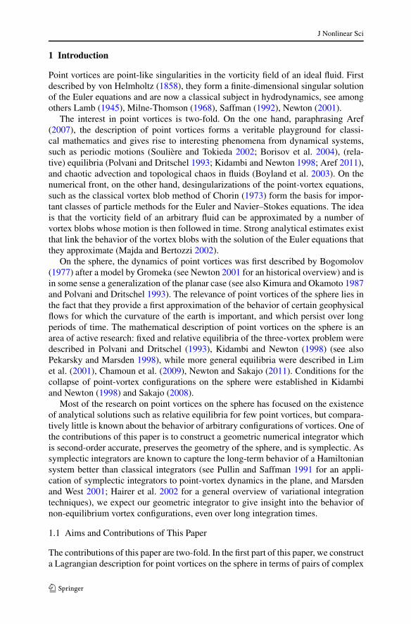
Polvani and Dritschel (1993) have investigated the behavior of a ring of N equidis-tant vortices with the same strength Γ , placed on a circle of fixed latitude on thesphere (see Fig. 1). They found that this configuration is a stable relative equi-librium, provided that N ≤ 7 and that the colatitude is below a certain criticalvalue (dependent on N ). For the case N = 6, the critical colatitude is given byθc = arccos(2/
√5) ≈ 0.464 and the stable relative equilibria satisfy θ0 < θc. The vor-
tex ring rotates around the z-axis with angular velocity Ω = (N − 1) Γ4π
z01−z2
0, where
z0 = cos θ0.For our simulation, we choose N = 6, Γ = 1/6 and θ0 = 0.40, so that Ω ≈ 0.397
and the period T ≈ 15.819. The motion of the first vortex over a number of periodsis illustrated in Fig. 1.
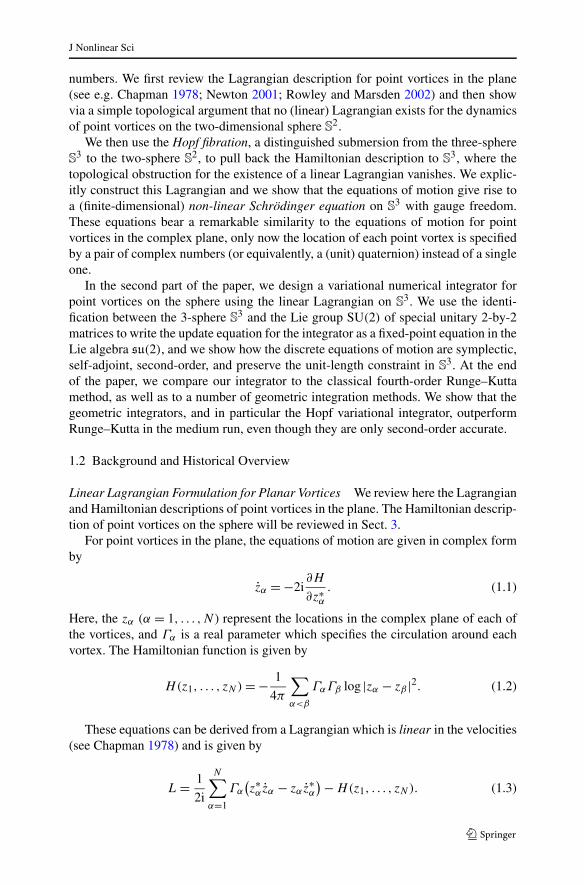
Comparison with Other Integrators We next turn to the energy and momentumconservation properties of the numerical integrator. We simulate the motion of thePolvani–Dritschel vortex ring with time step h = 0.1 and regularization parameterσ = 0.0, for T = 1000 units of time, using all four integrators.
In Fig. 2 we have plotted the absolute energy error �E := |E(tn) − E(t0)| (left)and the moment error �M := ‖M(tn) − M(t0)‖ (right) as a function of time. TheHopf integrator preserves the energy and vortex moment to machine precision, whilethe other three integrators exhibit drifts in both conserved quantities at various rates.
Numerical Order Calculation We know from theoretical considerations that theHopf integrator is second-order accurate, and so are the two other geometric methods.We now illustrate this statement by comparing the solution trajectories generated bythe Hopf integrator with the exact trajectories. For 10 choices of time step h between

J Nonlinear Sci
Fig. 1 Left: Initial conditions for the 6-vortex Polvani–Dritschel vortex ring. Right: x, y and z-componentof the first vortex in the Polvani–Dritschel simulation, where the time step h = 0.1. The trajectory is clearlyseen to be periodic
Fig. 2 Comparison of the energy and momentum preservation between all four methods for the stablePolvani–Dritschel vortex ring. The Hopf integrator preserves both invariants up to machine precision,while the other integrators exhibit a clear drift. Here h = 0.1 and σ = 0.0
10−4 and 10−1 we run the simulation over T = 100 units of time and we computethe absolute error between the numerical and the exact solution. We consider only thefirst vortex, since the trajectories of the other vortices differ from the first by a rigidrotation. More precisely, for each integrator we do the following: if xexact(tn) is theexact position of the first vortex at time tn = nh and xn,h
int is the numerical trajectory,then we compute
�h := maxn
∥∥xexact(tn) − xn,hint
∥∥
for each of the selected time steps. For the sake of comparison, we have also includedthe simulation results for the second-order Heun’s method composed with projectiononto S
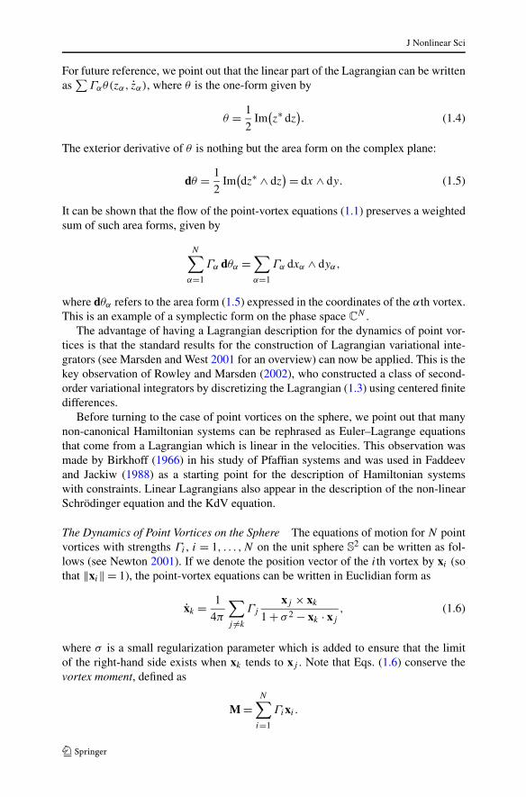
2, which is labeled on the figure as RK2.Figure 3 (left) shows a plot of absolute errors versus time steps for the three ge-
ometric integrators as well as RK2. All four integrators are of second-order. On theright pane of Fig. 3, we have plotted the obtained accuracy for each of the methodsas a function of the expended CPU time.
We see that, apart from a transient regime for large step sizes in which the Hopf in-tegrator is an order of magnitude slower, all three geometric methods perform compa-
J Nonlinear Sci
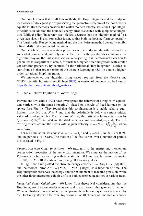
Fig. 3 Left: Absolute error for each of the four integrators for the Polvani–Dritschel vortex ring overT = 100 units of time. All four integrators are second-order accurate in time. Right: Absolute error as afunction of CPU time expended, again for T = 100 units of time. All three geometric integrators exhibitvery similar behavior in accuracy vs. computational cost, and Runge–Kutta is much cheaper than thegeometric integrators for the same accuracy
rably. In relative terms, RK2 clearly outperforms all three geometric methods, sincewith modest computational expense many orders of accuracy are obtained. This ispartly a result of the fact that the Polvani–Dritschel vortex ring is a relatively simple,periodic vortex system. We will see in the examples below that for non-equilibriumconfigurations, the energy and vortex moment slowly drift from their true valueswhen integrated with a non-symplectic integrator.
6.2 The Spherical von Kármán Vortex Street
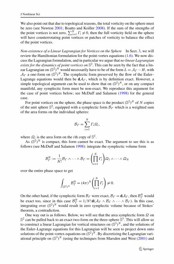
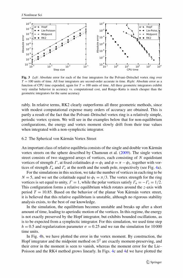
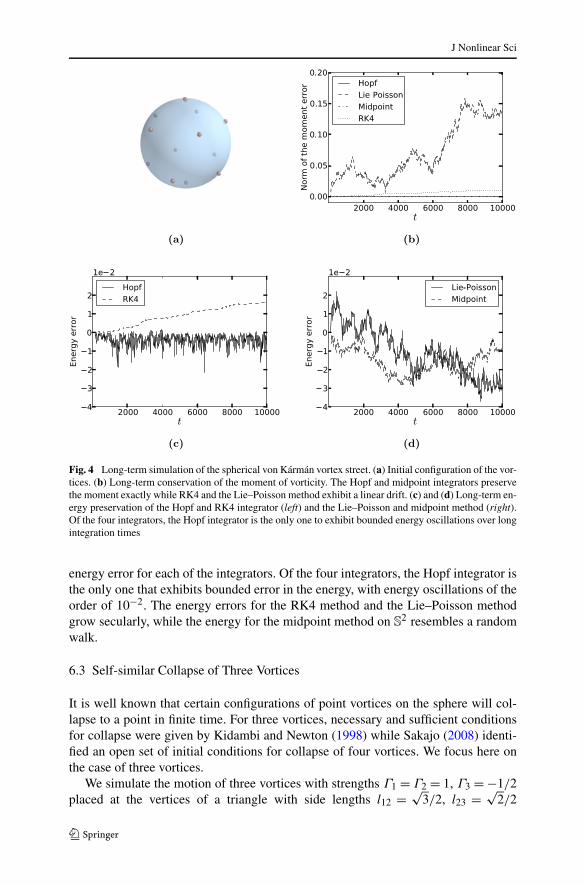
An important class of relative equilibria consists of the single and double von Kármánvortex streets on the sphere described by Chamoun et al. (2009). The single vortexstreet consists of two staggered arrays of vortices, each consisting of N equidistantvortices of strength Γ , at fixed colatitudes φ = φ1 and φ = π −φ1, together with vor-tices of strength Γn and Γs at the north and the south pole, respectively (see Fig. 4a).
For the simulations in this section, we take the number of vortices in each ring to beN = 5, and we set the colatitude equal to φ1 = π/3. The vortex strength for the ringvortices is set equal to unity, Γ = 1, while the polar vortices satisfy Γn = −Γs = 1/2.This configuration forms a relative equilibrium which rotates around the z-axis withperiod T = 10.85. Based on the behavior of the planar Von Kármán vortex street,it is believed that this relative equilibrium is unstable, although no rigorous stabilityanalysis exists, to the best of our knowledge.
In the simulation, the equilibrium becomes unstable and breaks up after a shortamount of time, leading to aperiodic motion of the vortices. In this regime, the energyis not exactly preserved by the Hopf integrator, but exhibits bounded oscillations, asis to be expected from a symplectic integrator. For this simulation, we used time steph = 0.5 and regularization parameter σ = 0.25 and we ran the simulation for 10 000time units.
In Fig. 4b, we have plotted the error in the vortex moment. By construction, theHopf integrator and the midpoint method on S
2 are exactly moment-preserving, andtheir error in the moment is seen to vanish, whereas the moment error for the Lie–Poisson and the RK4 method grows linearly. In Figs. 4c and 4d we have plotted the
J Nonlinear Sci
Fig. 4 Long-term simulation of the spherical von Kármán vortex street. (a) Initial configuration of the vor-tices. (b) Long-term conservation of the moment of vorticity. The Hopf and midpoint integrators preservethe moment exactly while RK4 and the Lie–Poisson method exhibit a linear drift. (c) and (d) Long-term en-ergy preservation of the Hopf and RK4 integrator (left) and the Lie–Poisson and midpoint method (right).Of the four integrators, the Hopf integrator is the only one to exhibit bounded energy oscillations over longintegration times
energy error for each of the integrators. Of the four integrators, the Hopf integrator isthe only one that exhibits bounded error in the energy, with energy oscillations of theorder of 10−2. The energy errors for the RK4 method and the Lie–Poisson methodgrow secularly, while the energy for the midpoint method on S
2 resembles a randomwalk.
6.3 Self-similar Collapse of Three Vortices
It is well known that certain configurations of point vortices on the sphere will col-lapse to a point in finite time. For three vortices, necessary and sufficient conditionsfor collapse were given by Kidambi and Newton (1998) while Sakajo (2008) identi-fied an open set of initial conditions for collapse of four vortices. We focus here onthe case of three vortices.
We simulate the motion of three vortices with strengths Γ1 = Γ2 = 1, Γ3 = −1/2placed at the vertices of a triangle with side lengths l12 = √
3/2, l23 = √2/2
J Nonlinear Sci
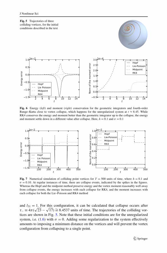
Fig. 5 Trajectories of threecolliding vortices, for the initialconditions described in the text
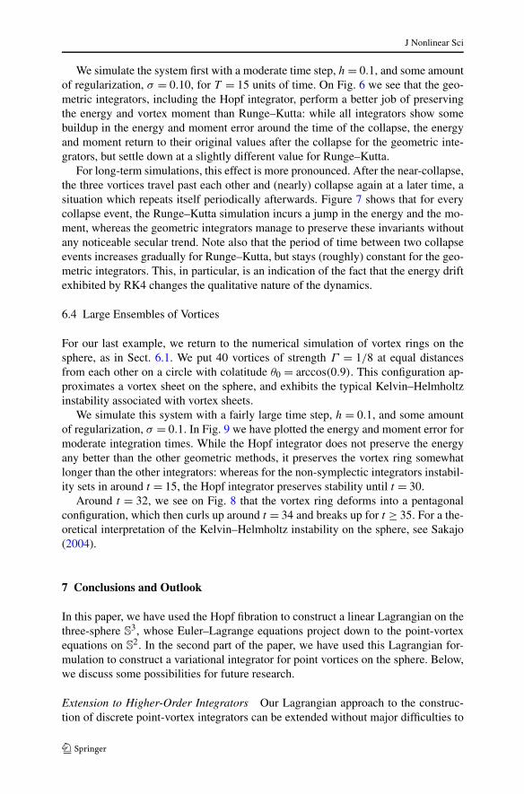
Fig. 6 Energy (left) and moment (right) conservation for the geometric integrators and fourth-orderRunge–Kutta close to vortex collapse, which happens for the unregularized system at t ≈ 8.45. WhileRK4 conserves the energy and moment better than the geometric integrator up to the collapse, the energyand moment settle down in a different value after collapse. Here, h = 0.1 and σ = 0.1
Fig. 7 Numerical simulation of colliding point vortices for T = 500 units of time, where h = 0.1 andσ = 0.10. At regular instances of time, there are collapse events, indicated by the spikes in the figures.Whereas the Hopf and the midpoint method preserve energy and the vortex moment reasonably well awayfrom collapse events, the energy increases with each collapse for RK4, and the moment increases witheach collapse for both the Lie–Poisson and RK4 method
and l31 = 1. For this configuration, it can be calculated that collapse occurs afterτ− ≡ 4π(
√23 − √
17) ∼= 8.4537 units of time. The trajectories of the colliding vor-tices are shown in Fig. 5. Note that these initial conditions are for the unregularizedsystem, i.e. (1.6) with σ = 0. Adding some regularization to the system effectivelyamounts to imposing a minimum distance on the vortices and will prevent the vortexconfiguration from collapsing to a single point.
J Nonlinear Sci
We simulate the system first with a moderate time step, h = 0.1, and some amountof regularization, σ = 0.10, for T = 15 units of time. On Fig. 6 we see that the geo-metric integrators, including the Hopf integrator, perform a better job of preservingthe energy and vortex moment than Runge–Kutta: while all integrators show somebuildup in the energy and moment error around the time of the collapse, the energyand moment return to their original values after the collapse for the geometric inte-grators, but settle down at a slightly different value for Runge–Kutta.
For long-term simulations, this effect is more pronounced. After the near-collapse,the three vortices travel past each other and (nearly) collapse again at a later time, asituation which repeats itself periodically afterwards. Figure 7 shows that for everycollapse event, the Runge–Kutta simulation incurs a jump in the energy and the mo-ment, whereas the geometric integrators manage to preserve these invariants withoutany noticeable secular trend. Note also that the period of time between two collapseevents increases gradually for Runge–Kutta, but stays (roughly) constant for the geo-metric integrators. This, in particular, is an indication of the fact that the energy driftexhibited by RK4 changes the qualitative nature of the dynamics.
6.4 Large Ensembles of Vortices
For our last example, we return to the numerical simulation of vortex rings on thesphere, as in Sect. 6.1. We put 40 vortices of strength Γ = 1/8 at equal distancesfrom each other on a circle with colatitude θ0 = arccos(0.9). This configuration ap-proximates a vortex sheet on the sphere, and exhibits the typical Kelvin–Helmholtzinstability associated with vortex sheets.
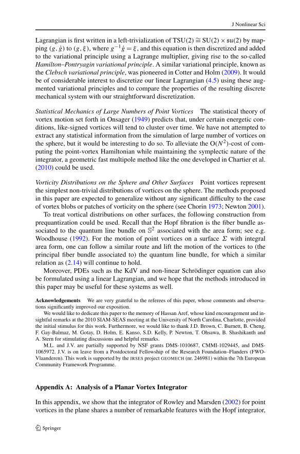
We simulate this system with a fairly large time step, h = 0.1, and some amountof regularization, σ = 0.1. In Fig. 9 we have plotted the energy and moment error formoderate integration times. While the Hopf integrator does not preserve the energyany better than the other geometric methods, it preserves the vortex ring somewhatlonger than the other integrators: whereas for the non-symplectic integrators instabil-ity sets in around t = 15, the Hopf integrator preserves stability until t = 30.
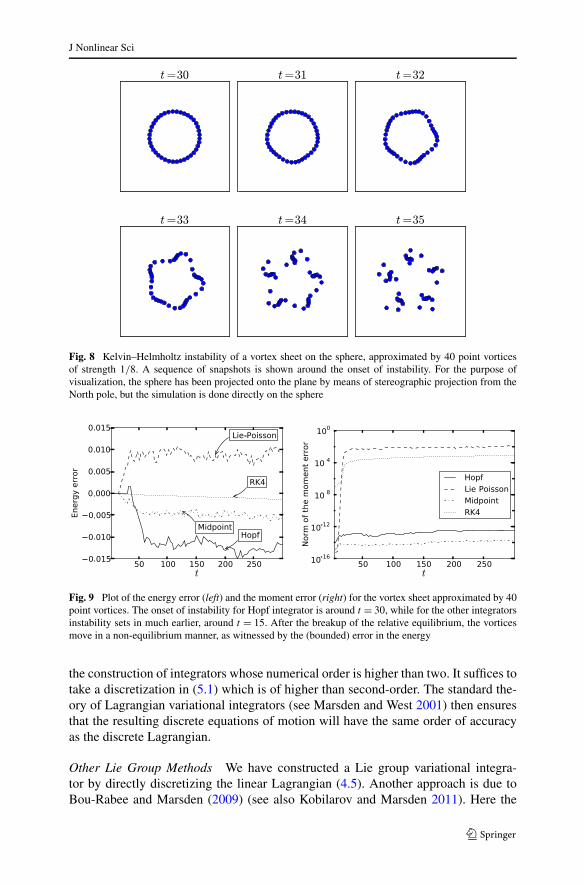
Around t = 32, we see on Fig. 8 that the vortex ring deforms into a pentagonalconfiguration, which then curls up around t = 34 and breaks up for t ≥ 35. For a the-oretical interpretation of the Kelvin–Helmholtz instability on the sphere, see Sakajo(2004).
7 Conclusions and Outlook
In this paper, we have used the Hopf fibration to construct a linear Lagrangian on thethree-sphere S
3, whose Euler–Lagrange equations project down to the point-vortexequations on S
2. In the second part of the paper, we have used this Lagrangian for-mulation to construct a variational integrator for point vortices on the sphere. Below,we discuss some possibilities for future research.
Extension to Higher-Order Integrators Our Lagrangian approach to the construc-tion of discrete point-vortex integrators can be extended without major difficulties to
J Nonlinear Sci
Fig. 8 Kelvin–Helmholtz instability of a vortex sheet on the sphere, approximated by 40 point vorticesof strength 1/8. A sequence of snapshots is shown around the onset of instability. For the purpose ofvisualization, the sphere has been projected onto the plane by means of stereographic projection from theNorth pole, but the simulation is done directly on the sphere
Fig. 9 Plot of the energy error (left) and the moment error (right) for the vortex sheet approximated by 40point vortices. The onset of instability for Hopf integrator is around t = 30, while for the other integratorsinstability sets in much earlier, around t = 15. After the breakup of the relative equilibrium, the vorticesmove in a non-equilibrium manner, as witnessed by the (bounded) error in the energy
the construction of integrators whose numerical order is higher than two. It suffices totake a discretization in (5.1) which is of higher than second-order. The standard the-ory of Lagrangian variational integrators (see Marsden and West 2001) then ensuresthat the resulting discrete equations of motion will have the same order of accuracyas the discrete Lagrangian.
Other Lie Group Methods We have constructed a Lie group variational integra-tor by directly discretizing the linear Lagrangian (4.5). Another approach is due toBou-Rabee and Marsden (2009) (see also Kobilarov and Marsden 2011). Here the
J Nonlinear Sci
Lagrangian is first written in a left-trivialization of TSU(2) ∼= SU(2)× su(2) by map-ping (g, g) to (g, ξ), where g−1g = ξ , and this equation is then discretized and addedto the variational principle using a Lagrange multiplier, giving rise to the so-calledHamilton–Pontryagin variational principle. A similar variational principle, known asthe Clebsch variational principle, was pioneered in Cotter and Holm (2009). It wouldbe of considerable interest to discretize our linear Lagrangian (4.5) using these aug-mented variational principles and to compare the properties of the resulting discretemechanical system with our straightforward discretization.
Statistical Mechanics of Large Numbers of Point Vortices The statistical theory ofvortex motion set forth in Onsager (1949) predicts that, under certain energetic con-ditions, like-signed vortices will tend to cluster over time. We have not attempted toextract any statistical information from the simulation of large number of vortices onthe sphere, but it would be interesting to do so. To alleviate the O(N2)-cost of com-puting the point-vortex Hamiltonian while maintaining the symplectic nature of theintegrator, a geometric fast multipole method like the one developed in Chartier et al.(2010) could be used.
Vorticity Distributions on the Sphere and Other Surfaces Point vortices representthe simplest non-trivial distributions of vortices on the sphere. The methods proposedin this paper are expected to generalize without any significant difficulty to the caseof vortex blobs or patches of vorticity on the sphere (see Chorin 1973; Newton 2001).
To treat vortical distributions on other surfaces, the following construction fromprequantization could be used. Recall that the Hopf fibration is the fiber bundle as-sociated to the quantum line bundle on S
2 associated with the area form; see e.g.Woodhouse (1992). For the motion of point vortices on a surface Σ with integralarea form, one can follow a similar route and lift the motion of the vortices to (theprincipal fiber bundle associated to) the quantum line bundle, for which a similarrelation as (2.14) will continue to hold.
Moreover, PDEs such as the KdV and non-linear Schrödinger equation can alsobe formulated using a linear Lagrangian, and we hope that the methods introduced inthis paper may be useful for these systems as well.
Acknowledgements We are very grateful to the referees of this paper, whose comments and observa-tions significantly improved our exposition.
We would like to dedicate this paper to the memory of Hassan Aref, whose kind encouragement and in-sightful remarks at the 2010 SIAM-SEAS meeting at the University of North Carolina, Charlotte, providedthe initial stimulus for this work. Furthermore, we would like to thank J.D. Brown, C. Burnett, B. Cheng,F. Gay-Balmaz, M. Gotay, D. Holm, E. Kanso, S.D. Kelly, P. Newton, T. Ohsawa, B. Shashikanth andA. Stern for stimulating discussions and helpful remarks.
M.L. and J.V. are partially supported by NSF grants DMS-1010687, CMMI-1029445, and DMS-1065972. J.V. is on leave from a Postdoctoral Fellowship of the Research Foundation–Flanders (FWO-Vlaanderen). This work is supported by the IRSES project GEOMECH (nr. 246981) within the 7th EuropeanCommunity Framework Programme.
Appendix A: Analysis of a Planar Vortex Integrator
In this appendix, we show that the integrator of Rowley and Marsden (2002) for pointvortices in the plane shares a number of remarkable features with the Hopf integrator,
J Nonlinear Sci
which stems from the fact that both systems are derivable from a linear Lagrangian.Similar observations, but for the numerical integration of canonical Hamiltonian sys-tems, were made by Brown (2006).
Decomposition into One-Step Methods Rowley and Marsden (2002) start from thelinear Lagrangian (1.3), which they discretize by setting
Ld(z0, z1) = hL
((1 − α)z0 + αz1,
z1 − z0
h
),
where α ∈ [0,1] is a real interpolation parameter. The equations of motion derivedfrom this Lagrangian are given by
zn+2 − zn
2h= αf (zn+α) + (1 − α)f (zn+1+α), (A.1)
where zn+α := (1 − α)zn + αzn+1 and f (z) is the right-hand side of the vortex equa-tions (1.1). It turns out that for α = 1/2, they can be written as the composition of aone-step method and its adjoint. To see this, we specialize to the case α = 1/2 anduse the fact that the original Lagrangian L is linear in the velocities to write
Ld(z0, z1) = L(z1/2, z1) − L(z1/2, z0),
and we define Ld,+(z0, z1, h) := L(z1/2, z1) and Ld,−(z0, z1, h) := −L(z1/2, z0), sothat Ld = Ld,+ + Ld,−. Consider the adjoint L∗
d of a discrete Lagrangian Ld, whichis defined by L∗
d(z0, z1, h) := −Ld(z1, z0,−h) (see Marsden and West 2001). Then,we have
L∗d,+(z0, z1, h) = Ld,−(z0, z1, h),
and vice versa. This definition is motivated by the fact that the adjoint of the dis-crete Euler–Lagrange flow of a discrete Lagrangian is given by the discrete Euler–Lagrange flow of the adjoint discrete Lagrangian.
The composition of the discrete Euler–Lagrange flow of two discrete Lagrangiansis given by the discrete Euler–Lagrange flow of a composition discrete Lagrangianthat is the sum of the two original discrete Lagrangians. As a result, the discreteEuler–Lagrange flow for Ld is given by the composition of the discrete Euler–Lagrange flows for Ld,+ and its adjoint L∗
d,+ = Ld,−. These discrete flows can beviewed as one-step methods, and are typically only first-order accurate, but their com-position is symmetric and therefore has even order of accuracy, and is, in particular,second-order accurate.
Lastly, we remark that for the point-vortex Lagrangian (1.3) the discrete La-grangians Ld,+ and Ld,− coincide, which means that each of them is individuallyself-adjoint. As a result, the underlying one-step method is second-order. In fact, itcan easily be seen that for α = 1/2, the point-vortex equations (A.1) can be writtenas the composition of the implicit midpoint method
zn+1 − zn
h= f (zn+1/2)
J Nonlinear Sci
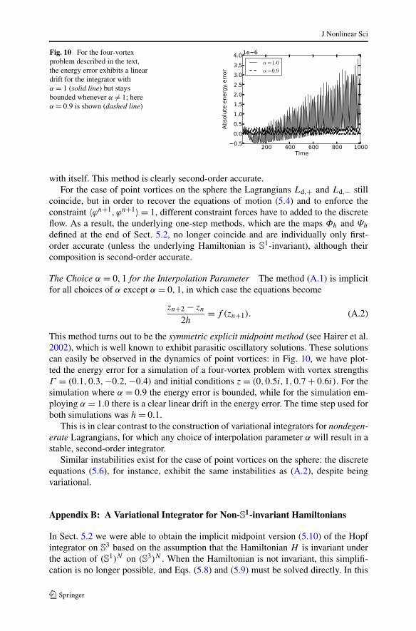
Fig. 10 For the four-vortexproblem described in the text,the energy error exhibits a lineardrift for the integrator withα = 1 (solid line) but staysbounded whenever α �= 1; hereα = 0.9 is shown (dashed line)
with itself. This method is clearly second-order accurate.For the case of point vortices on the sphere the Lagrangians Ld,+ and Ld,− still
coincide, but in order to recover the equations of motion (5.4) and to enforce theconstraint 〈ϕn+1, ϕn+1〉 = 1, different constraint forces have to added to the discreteflow. As a result, the underlying one-step methods, which are the maps Φh and Ψh
defined at the end of Sect. 5.2, no longer coincide and are individually only first-order accurate (unless the underlying Hamiltonian is S
1-invariant), although theircomposition is second-order accurate.
The Choice α = 0,1 for the Interpolation Parameter The method (A.1) is implicitfor all choices of α except α = 0,1, in which case the equations become
zn+2 − zn
2h= f (zn+1). (A.2)
This method turns out to be the symmetric explicit midpoint method (see Hairer et al.2002), which is well known to exhibit parasitic oscillatory solutions. These solutionscan easily be observed in the dynamics of point vortices: in Fig. 10, we have plot-ted the energy error for a simulation of a four-vortex problem with vortex strengthsΓ = (0.1,0.3,−0.2,−0.4) and initial conditions z = (0,0.5i,1,0.7 + 0.6i). For thesimulation where α = 0.9 the energy error is bounded, while for the simulation em-ploying α = 1.0 there is a clear linear drift in the energy error. The time step used forboth simulations was h = 0.1.
This is in clear contrast to the construction of variational integrators for nondegen-erate Lagrangians, for which any choice of interpolation parameter α will result in astable, second-order integrator.
Similar instabilities exist for the case of point vortices on the sphere: the discreteequations (5.6), for instance, exhibit the same instabilities as (A.2), despite beingvariational.
Appendix B: A Variational Integrator for Non-S1-invariant Hamiltonians
In Sect. 5.2 we were able to obtain the implicit midpoint version (5.10) of the Hopfintegrator on S
3 based on the assumption that the Hamiltonian H is invariant underthe action of (S1)N on (S3)N . When the Hamiltonian is not invariant, this simplifi-cation is no longer possible, and Eqs. (5.8) and (5.9) must be solved directly. In this
J Nonlinear Sci
appendix, we outline a strategy for doing so, based on the geometry of the groupSU(2).
Implementing the Unit-Length Constraint: The Cayley Map Given initial conditions(ϕn−1, ϕn), we first compute the slack variables dn
α using (5.9). We must now solve(5.8) for ϕn+1, and we need to impose the unit-length constraint (5.5). This can bedone conveniently using the geometry of SU(2): we write the update map ϕn → ϕn+1
as
ϕn+1 = Unϕn, (B.1)
where Un is an element of SU(2). This ensures that the length of ϕn stays constantover time, since
(ϕn+1)†
ϕn+1 = (ϕn
)†(Un
)†Unϕn = (
ϕn)†
ϕn,
so that, in particular, ‖ϕn‖ = 1 implies that ‖ϕn+1‖ = 1.Equations (5.8) for ϕn+1 can now be expressed as
Re
[(ϕn
)†(iσα)
(−iΓ
(Un − I2×2
)ϕn + h
2Dϕ†H
(ϕn+1/2)
)]= −dn
α, (B.2)
where ϕn+1/2 in the Hamiltonian can be expressed in terms of Un and ϕn by
ϕn+1/2 = 1
2
(ϕn + ϕn+1) = 1
2
(I + Un
)ϕn.
These equations can be solved for Un directly, but a computationally more advan-tageous approach is as follows. As long as the step size h is small, the update matrixUn will be in a neighborhood of the identity element in SU(2). We now parametrizethat neighborhood by means of the Cayley transform Cay : su(2) → SU(2), given by
Cay(A) = (I + A)(I − A)−1.
That is, we search for an element An ∈ su(2) such that Un = Cay(An) will solve(B.2). The advantage is that su(2) is a linear space, and that no constraints needto be imposed on An, as the range of the Cayley map is automatically containedwithin SU(2). A standard non-linear solver can therefore be used to find An. Thisis analogous to the approach used in Lee et al. (2009) to implement the unit-lengthconstraint on S2 by updating the solution on the sphere using a SO(3) action that isparametrized by the Cayley transform from so(3) to SO(3).
Computational Savings Significant computational savings can be obtained byrewriting the Cayley map in a more convenient form. We recall from (2.6) that su(2)
is isomorphic with R3, and we denote the vector representation of An by an ∈ R
3.A small calculation then shows that the Cayley transform can be expressed as
Un = Cay(An
) = 1
1 + ‖an‖2
((1 − ∥∥an
∥∥2)I + 2An
), (B.3)

J Nonlinear Sci
so that
Un − I2×2 = 2
1 + ‖an‖2
(An − ∥∥an
∥∥2I2×2
).
The terms proportional to Γ in (B.2) can then be written as
Re[Γ
(ϕn
)†σα
(Un − I2×2
)ϕn
]
= 2Γ
1 + ‖an‖2Re
[(ϕn
)†σα
(An − ∥∥an
∥∥2I2×2
)ϕn
]
= 2Γ
1 + ‖an‖2
(Re
[(ϕn
)†σαAnϕn
] − ∥∥an∥∥2 Re
[(ϕn
)†σαϕn
])
= −2Γ
1 + ‖an‖2
(an × xn + ∥∥an
∥∥2xn)α, (B.4)
where we have used the expression (2.11) for the Hopf fibration to write xnα =
(ϕn)†σαϕn, as well as the identity
(ϕn
)†σαAnϕn = i
3∑
β=1
(an
)β
(ϕn
)†σασβϕn
= i(an
)α
− (an × xn
)α,
which follows easily from (2.7).Similarly, the terms in (B.2) involving the derivatives of the Hamiltonian can be
written using (4.13) as
Re((
ϕn)†
(iσα)Dϕ†H(ϕn+1/2))
= 1
1 + ‖an‖2
(xn × ∇H
n+1/2S2 − (
an · xn)∇H
n+1/2S2 − (
an × xn) × ∇H
n+1/2S2
)α,
where HS2 is the original point-vortex Hamiltonian (3.2).Combining this expression with (B.4), we see that the first-order equations (B.2)
for Un are equivalent to the following non-linear equation for an:
− 2Γ(an × xn + ∥∥an
∥∥2xn) + h
2
(xn × ∇H
n+1/2S2 − (
an · xn)∇H
n+1/2S2
− (an × xn
) × ∇Hn+1/2S2
)
= −(1 + ∥∥an
∥∥2)dn. (B.5)
The first-order equations (5.9) can be rewritten in a similar fashion as a vectorequation involving xn−1,xn and an−1. However, as there is no need to solve theseequations directly (they merely serve to determine the slack variable dn), we will notgo in further detail.
J Nonlinear Sci
Summary To solve the discrete equations of motion (5.8) and (5.9) in the case of anon-S1-invariant Hamiltonian, we proceed as follows:
1. Given initial conditions (ϕn−1, ϕn) ∈ S3 × S
3, compute the slack dn from (5.9).2. For this dn, find an from (B.5).3. Once an is known, update ϕn to find ϕn+1 using the Cayley map (B.1).
The advantage of computing ϕn+1 indirectly via an is that (B.5) is a non-linearequation defined on su(2)N . As this is a vector space, a standard non-linear solvercan be used to solve (B.5). While Owren and Welfert (2000) developed an extensionof Newton’s method that preserves the Lie group structure, it is much more compu-tationally involved.
References
Aref, H.: Point vortex dynamics: a classical mathematics playground. J. Math. Phys. 48, 065401 (2007)Aref, H.: Relative equilibria of point vortices and the fundamental theorem of algebra. Proc. R. Soc. A,
Math. Phys. Eng. Sci. 467, 2168–2184 (2011)Benettin, G., Giorgilli, A.: On the Hamiltonian interpolation of near to the identity symplectic mappings
with application to symplectic integration algorithms. J. Stat. Phys. 74, 1117–1143 (1994)Birkhoff, G.D.: Dynamical Systems. American Mathematical Society Colloquium Publications, vol. IX.
American Mathematical Society, Providence (1966). With an addendum by Jurgen MoserBoatto, S., Koiller, J.: Vortices on closed surfaces. Preprint. arXiv:0802.4313v1 (2008)Bogomolov, V.A.: Dynamics of vorticity at a sphere. Fluid Dyn. 12, 863–870 (1977). doi:10.1007/
BF01090320Borisov, A.V., Mamaev, I.S., Kilin, A.A.: Absolute and relative choreographies in the problem of point
vortices moving on a plane. Regul. Chaotic Dyn. 9, 101–111 (2004)Bou-Rabee, N., Marsden, J.E.: Hamilton–Pontryagin integrators on Lie groups. I. Introduction and
structure-preserving properties. Found. Comput. Math. 9, 197–219 (2009)Boyland, P., Stremler, M., Aref, H.: Topological fluid mechanics of point vortex motions. Physica D 175,
69–95 (2003)Brown, J.D.: Midpoint rule as a variational-symplectic integrator: Hamiltonian systems. Phys. Rev. D 73,
024001 (2006)Bruveris, M., Ellis, D.C.P., Holm, D.D., Gay-Balmaz, F.: Un-reduction. J. Geom. Mech. 3, 363–387 (2011)Cendra, H., Marsden, J.E.: Lin constraints, Clebsch potentials and variational principles. Physica D 27,
63–89 (1987)Chamoun, G., Kanso, E., Newton, P.K.: Von Kármán vortex streets on the sphere. Phys. Fluids 21, 116603
(2009)Chapman, D.M.F.: Ideal vortex motion in two dimensions: symmetries and conservation laws. J. Math.
Phys. 19, 1988–1992 (1978)Chartier, P., Darrigrand, E., Faou, E.: A regular fast multipole method for geometric numerical integrations
of Hamiltonian systems. BIT Numer. Math. 50, 23–40 (2010)Chorin, A.J.: Numerical study of slightly viscous flow. J. Fluid Mech. 57, 785–796 (1973)Cotter, C.J., Holm, D.D.: Continuous and discrete Clebsch variational principles. Found. Comput. Math.
9, 221–242 (2009)Engø, K., Faltinsen, S.: Numerical integration of Lie–Poisson systems while preserving coadjoint orbits
and energy. SIAM J. Numer. Anal. 39, 128–145 (2002)Faddeev, L., Jackiw, R.: Hamiltonian reduction of unconstrained and constrained systems. Phys. Rev. Lett.
60, 1692–1694 (1988)Frankel, T.: The Geometry of Physics: An Introduction, 2nd edn. Cambridge University Press, Cambridge
(2004)Gotay, M.: Presymplectic manifolds, geometric constraint theory and the Dirac-Bergmann theory of con-
straints. PhD thesis, University of Maryland (1979)
J Nonlinear Sci
Hairer, E.: Backward analysis of numerical integrators and symplectic methods. Ann. Numer. Math. 1,107–132 (1994)
Hairer, E., Lubich, C.: The life-span of backward error analysis for numerical integrators. Numer. Math.76, 441–462 (1997)
Hairer, E., Lubich, C., Wanner, G.: Geometric Numerical Integration, 1st edn. Springer Series in Compu-tational Mathematics, vol. 31. Springer, Berlin (2002)
Khesin, B.: Symplectic structures and dynamics on vortex membranes. Mosc. Math. J. 12, 413–434 (2012).461–462
Kidambi, R., Newton, P.K.: Motion of three point vortices on a sphere. Physica D 116, 143–175 (1998)Kimura, Y., Okamoto, H.: Vortex motion on a sphere. J. Phys. Soc. Jpn. 56, 4203–4206 (1987)Kobilarov, M., Marsden, J.: Discrete geometric optimal control on Lie groups. IEEE Trans. Robot. 27,
641–655 (2011)Kostant, B.: Minimal coadjoint orbits and symplectic induction. In: The Breadth of Symplectic and Poisson
Geometry. Progr. Math., vol. 232, pp. 391–422. Birkhäuser, Boston (2005)Lamb, H.: Hydrodynamics. Dover Publications, New York (1945). Reprint of the 1932 Cambridge Uni-
versity Press editionLee, T., Leok, M., McClamroch, N.H.: Lie group variational integrators for the full body problem. Comput.
Methods Appl. Mech. Eng. 196, 2907–2924 (2007)Lee, T., Leok, M., McClamroch, N.H.: Lagrangian mechanics and variational integrators on two-spheres.
Int. J. Numer. Methods Eng. 79, 1147–1174 (2009)Lemaître, G.: Quaternions et espace elliptique. Pont. Acad. Sci. Acta 12, 57–78 (1948)Leok, M., Zhang, J.: Discrete Hamiltonian variational integrators. IMA J. Numer. Anal. 31, 1497–1532
(2011)Leyendecker, S., Marsden, J.E., Ortiz, M.: Variational integrators for constrained dynamical systems. Z.
Angew. Math. Mech. 88, 677–708 (2008)Lim, C., Montaldi, J., Roberts, M.: Relative equilibria of point vortices on the sphere. Physica D 148,
97–135 (2001)Ma, Z., Rowley, C.W.: Lie-Poisson integrators: a Hamiltonian, variational approach. Int. J. Numer. Meth-
ods Eng. 82, 1609–1644 (2010)Majda, A.J., Bertozzi, A.L.: Vorticity and Incompressible Flow. Cambridge Texts in Applied Mathematics,
vol. 27. Cambridge University Press, Cambridge (2002)Marsden, J.E., West, M.: Discrete mechanics and variational integrators. Acta Numer. 10, 357–514 (2001)McDuff, D., Salamon, D.: Introduction to Symplectic Topology, 2nd edn. Oxford Mathematical Mono-
graphs. The Clarendon Press Oxford University Press, New York (1998)Milne-Thomson, L.: Theoretical Hydrodynamics, 5th edn. MacMillan and Co. Ltd., London (1968). Re-
vised and enlarged editionMontgomery, R.: A Tour of Subriemannian Geometries, Their Geodesics and Applications. Mathematical
Surveys and Monographs, vol. 91. American Mathematical Society, Providence (2002)Moser, J., Veselov, A.: Discrete versions of some classical integrable systems and factorization of matrix
polynomials. Commun. Math. Phys. 139, 217–243 (1991)Newton, P.K.: The N -Vortex Problem. Analytical Techniques. Applied Mathematical Sciences, vol. 145.
Springer, New York (2001)Newton, P.K., Sakajo, T.: Point vortex equilibria and optimal packings of circles on a sphere. Proc. R. Soc.
A, Math. Phys. Eng. Sci. 467, 1468–1490 (2011)Novikov, S.P.: The Hamiltonian formalism and a many-valued analogue of Morse theory. Russ. Math.
Surv. 37, 1 (1982)Oh, Y.-G.: Symplectic topology as the geometry of action functional. I. Relative Floer theory on the cotan-
gent bundle. J. Differ. Geom. 46, 499–577 (1997)Oliphant, T.E.: Python for scientific computing. Comput. Sci. Eng. 9, 10–20 (2007)Onsager, L.: Statistical hydrodynamics. Nuovo Cimento 6, 279–287 (1949)Owren, B., Welfert, B.: The Newton iteration on Lie groups. BIT Numer. Math. 40, 121–145 (2000)Pekarsky, S., Marsden, J.E.: Point vortices on a sphere: stability of relative equilibria. J. Math. Phys. 39,
5894–5907 (1998)Polvani, L.M., Dritschel, D.G.: Wave and vortex dynamics on the surface of a sphere. J. Fluid Mech. 255,
35–64 (1993)Pullin, D.I., Saffman, P.G.: Long-time symplectic integration: the example of four-vortex motion. Proc.
Math. Phys. Sci. 432, 481–494 (1991)Reich, S.: Backward error analysis for numerical integrators. SIAM J. Numer. Anal. 36, 1549–1570 (1999)
J Nonlinear Sci
Rowley, C., Marsden, J.: Variational integrators for degenerate Lagrangians, with application to pointvortices. In: Proceedings of the 41st IEEE Conference on Decision and Control, vol. 2, pp. 1521–1527 (2002)
Saffman, P.G.: Vortex Dynamics. Cambridge Monographs on Mechanics and Applied Mathematics. Cam-bridge University Press, New York (1992)
Sakajo, T.: Motion of a vortex sheet on a sphere with pole vortices. Phys. Fluids 16, 717–727 (2004)Sakajo, T.: Non-self-similar, partial, and robust collapse of four point vortices on a sphere. Phys. Rev. E
78, 016312 (2008)Shashikanth, B.N.: Vortex dynamics in R
4. J. Math. Phys. 53, 013103, 21 (2012)Soulière, A., Tokieda, T.: Periodic motions of vortices on surfaces with symmetry. J. Fluid Mech. 460,
83–92 (2002)Urbantke, H.K.: The Hopf fibration—seven times in physics. J. Geom. Phys. 46, 125–150 (2003)von Helmholtz, H.: Über Integrale der hydro-dynamischen Gleichungen, welche den Wirbelbewegungen
entsprechen. J. Reine Angew. Math. 55, 25–55 (1858)Woodhouse, N.M.J.: Geometric Quantization, 2nd edn. Oxford Mathematical Monographs. The Clarendon
Press Oxford University Press, New York (1992)Zhong, G., Marsden, J.E.: Lie-Poisson Hamilton-Jacobi theory and Lie-Poisson integrators. Phys. Lett. A
133, 134–139 (1988)