a novel dementia diagnosis strategy on arterial spin

Multimed Tools Appl (2016) 75:2067–2090DOI 10.1007/s11042-014-2395-2

A novel dementia diagnosis strategy on arterial spinlabeling magnetic resonance images via pixel-wise partialvolume correction and ranking

Wei Huang ·Peng Zhang ·Minmin Shen

Received: 11 July 2014 / Revised: 9 October 2014 / Accepted: 24 November 2014 /Published online: 6 December 2014© Springer Science+Business Media New York 2014

Abstract Arterial Spin Labeling (ASL) is an emerging magnetic resonance imaging tech-nique attracting increasing attention in dementia diagnosis only beginning from recentyears. ASL is capable to provide direct and quantitative measurement of cerebral blood flow(CBF) of scanned patients, so that brain atrophy of demented patients could be revealedby measured low CBF within certain brain regions through ASL. However, partial volumeeffects (PVE) mainly caused by signal cross-contamination due to pixel heterogeneity andlimited spatial resolution of ASL, often prevents CBF from being precisely measured. Inac-curate CBF is prone to mislead and even deteriorate dementia disease diagnosis results,thereafter. In this paper, a novel dementia disease diagnosis strategy based on ASL is pro-posed for the first time. The diagnosis strategy is composed of two steps: 1) to conductpixel-wise PVE correction on original ASL images and 2) to predict dementia disease sever-ities based on corrected ASL images via ranking. Extensive experiments and comprehensivestatistical analysis are carried out to demonstrate the superiority of the new strategy withcomparison to several existing ones. Promising results are reported from the statistical pointof view.

Keywords Magnetic resonance image · Alzheimer’s disease · Ranking

W. Huang ()School of Information Engineering, Nanchang University, Nanchang, Chinae-mail: [email protected]

P. Zhang ()School of Computer Science, Northwestern Polytechnical University, Xi’an, Chinae-mail: [email protected]

M. ShenINCIDE Center, University of Konstanz, Konstanz, Germanye-mail: [email protected]

M. ShenSchool of Software Engineering, South China University of Technology, Guangzhou, China

mailto:[email protected]



2068 Multimed Tools Appl (2016) 75:2067–2090

1 Introduction

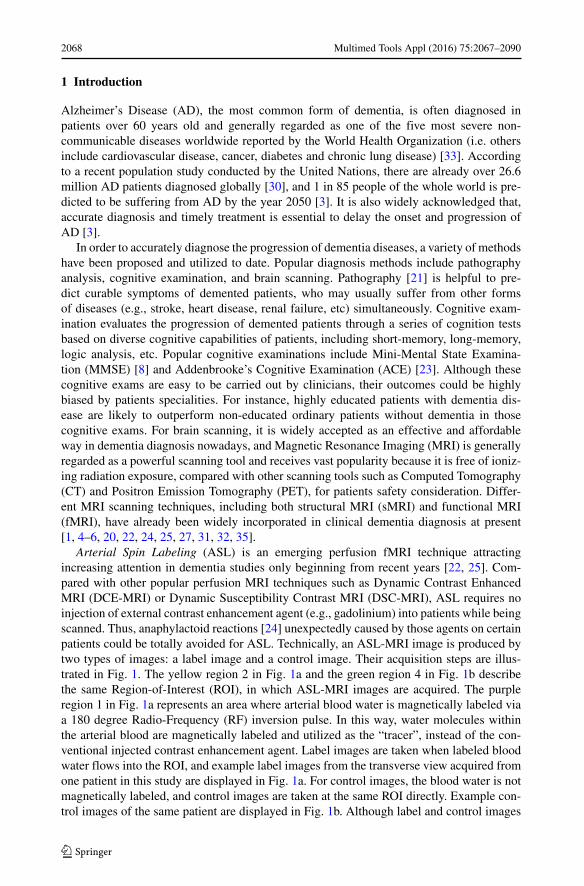
Alzheimer’s Disease (AD), the most common form of dementia, is often diagnosed inpatients over 60 years old and generally regarded as one of the five most severe non-communicable diseases worldwide reported by the World Health Organization (i.e. othersinclude cardiovascular disease, cancer, diabetes and chronic lung disease) [33]. Accordingto a recent population study conducted by the United Nations, there are already over 26.6million AD patients diagnosed globally [30], and 1 in 85 people of the whole world is pre-dicted to be suffering from AD by the year 2050 [3]. It is also widely acknowledged that,accurate diagnosis and timely treatment is essential to delay the onset and progression ofAD [3].

In order to accurately diagnose the progression of dementia diseases, a variety of methodshave been proposed and utilized to date. Popular diagnosis methods include pathographyanalysis, cognitive examination, and brain scanning. Pathography [21] is helpful to pre-dict curable symptoms of demented patients, who may usually suffer from other formsof diseases (e.g., stroke, heart disease, renal failure, etc) simultaneously. Cognitive exam-ination evaluates the progression of demented patients through a series of cognition testsbased on diverse cognitive capabilities of patients, including short-memory, long-memory,logic analysis, etc. Popular cognitive examinations include Mini-Mental State Examina-tion (MMSE) [8] and Addenbrooke’s Cognitive Examination (ACE) [23]. Although thesecognitive exams are easy to be carried out by clinicians, their outcomes could be highlybiased by patients specialities. For instance, highly educated patients with dementia dis-ease are likely to outperform non-educated ordinary patients without dementia in thosecognitive exams. For brain scanning, it is widely accepted as an effective and affordableway in dementia diagnosis nowadays, and Magnetic Resonance Imaging (MRI) is generallyregarded as a powerful scanning tool and receives vast popularity because it is free of ioniz-ing radiation exposure, compared with other scanning tools such as Computed Tomography(CT) and Positron Emission Tomography (PET), for patients safety consideration. Differ-ent MRI scanning techniques, including both structural MRI (sMRI) and functional MRI(fMRI), have already been widely incorporated in clinical dementia diagnosis at present[1, 4–6, 20, 22, 24, 25, 27, 31, 32, 35].

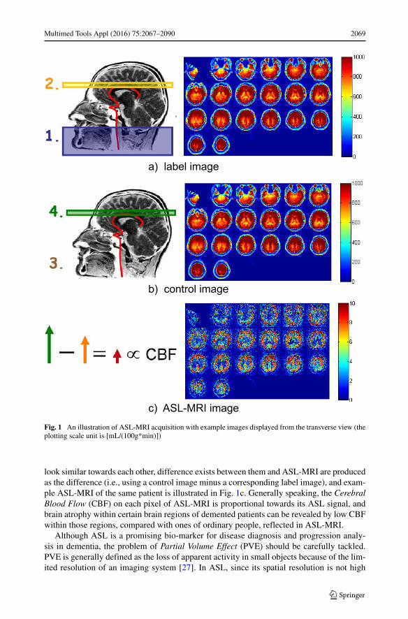
Arterial Spin Labeling (ASL) is an emerging perfusion fMRI technique attractingincreasing attention in dementia studies only beginning from recent years [22, 25]. Com-pared with other popular perfusion MRI techniques such as Dynamic Contrast EnhancedMRI (DCE-MRI) or Dynamic Susceptibility Contrast MRI (DSC-MRI), ASL requires noinjection of external contrast enhancement agent (e.g., gadolinium) into patients while beingscanned. Thus, anaphylactoid reactions [24] unexpectedly caused by those agents on certainpatients could be totally avoided for ASL. Technically, an ASL-MRI image is produced bytwo types of images: a label image and a control image. Their acquisition steps are illus-trated in Fig. 1. The yellow region 2 in Fig. 1a and the green region 4 in Fig. 1b describethe same Region-of-Interest (ROI), in which ASL-MRI images are acquired. The purpleregion 1 in Fig. 1a represents an area where arterial blood water is magnetically labeled viaa 180 degree Radio-Frequency (RF) inversion pulse. In this way, water molecules withinthe arterial blood are magnetically labeled and utilized as the “tracer”, instead of the con-ventional injected contrast enhancement agent. Label images are taken when labeled bloodwater flows into the ROI, and example label images from the transverse view acquired fromone patient in this study are displayed in Fig. 1a. For control images, the blood water is notmagnetically labeled, and control images are taken at the same ROI directly. Example con-trol images of the same patient are displayed in Fig. 1b. Although label and control images

Multimed Tools Appl (2016) 75:2067–2090 2069

Fig. 1 An illustration of ASL-MRI acquisition with example images displayed from the transverse view (theplotting scale unit is [mL/(100g*min)])

look similar towards each other, difference exists between them and ASL-MRI are producedas the difference (i.e., using a control image minus a corresponding label image), and exam-ple ASL-MRI of the same patient is illustrated in Fig. 1c. Generally speaking, the CerebralBlood Flow (CBF) on each pixel of ASL-MRI is proportional towards its ASL signal, andbrain atrophy within certain brain regions of demented patients can be revealed by low CBFwithin those regions, compared with ones of ordinary people, reflected in ASL-MRI.

Although ASL is a promising bio-marker for disease diagnosis and progression analy-sis in dementia, the problem of Partial Volume Effect (PVE) should be carefully tackled.PVE is generally defined as the loss of apparent activity in small objects because of the lim-ited resolution of an imaging system [27]. In ASL, since its spatial resolution is not high


(i.e., it can be perceived by example images in Fig. 1), pixels in ASL-MRI images contain-ing various tissues of Gray Matter (GM), White Matter (WM) and Cerebro-Spinal Fluid(CSF) are likely to be assigned with under-estimated ASL signal and low CBF quantities,which reflects the loss of apparent activity in ASL-MRI because of PVE. In order to correctPVE, there are already several studies conducted in recent years [1, 5, 6], and the regression-based method receives much popularity among them [1]. However, its shortcoming is alsoobvious. Neighboring pixels are usually indispensable for PVE correction on each singlepixel of ASL-MRI, making blurring and loss of brain details inevitable in correction resultsof this method [1]. A case in point is illustrated in the 1st row of Fig. 2. Therefore, in orderto enable ASL a reliable indicator for the following dementia diagnosis, the problem of PVEneeds to be properly handled first.

After PVE correction on ASL-MRI is conducted, the next critical step in dementia diag-nosis is to predict the dementia disease severity based on corrected ASL-MRI of eachpatient. Dementia studies incorporating ASL-MRI only begin to emerge in recent years[4, 22, 25, 31], and most of them concentrate on verifying ASL-MRI as a new indica-tor in identifying dementia disease, with comparison to other previously well-establishedimaging modalities (e.g. PET [25] and FDG-PET, which is short for Fludeoxyglucose-PET[4, 31]). For the majority of contemporary dementia disease diagnosis studies, they mainlyrely on conventional pattern recognition tools [20, 32, 35]. For instance, cortical thicknessmaps are generated from sMRI and Support Vector Machine (SVM) is employed to differ-entiateMild Cognitive Impairment (MCI) from AD in [32]. In [20], the curse-of-dimensionproblem commonly seen in pattern recognition studies is investigated in dementia diagnosis,and ensemble classifiers are constructed via sparse encodings for dementia disease predic-tion. In [35], local volumetric measurements obtained from sMRI are fed into hierarchicalnetworks to discern MCI patients from AD patients. It can be summarized from existing

Fig. 2 An Example of PVE correction results via the compared regression-based method (1st row) and thepixel-wise correction method (2nd) on the same patient (the plotting scale unit is [mL/(100g*min)])


studies that, dementia disease prediction is often considered as either a classification or aregression problem.

In this study, a novel dementia diagnosis strategy based on ASL-MRI is introduced forthe first time. The strategy is composed of two steps. The first step is to introduce a novelpixel-wise PVE correction method, which only incorporates information extracted from onesingle pixel for its own PVE correction, rather than information from both a pixel itselfand its neighboring pixels commonly adopted in contemporary PVE correction methods[1, 5, 6]. Existing problems such as blurring and brain details loss commonly seen in cor-rection results of those contemporary PVE correction methods can be properly tackled, andunder-estimated CBF in ASL-MRI can be well improved. The second step is to present anovel dementia disease prediction method based on corrected ASL-MRI from a new per-spective of ranking, instead of the conventional classification and regression viewpoints incontemporary studies [20, 32, 35]. The reason to conduct dementia disease prediction viaranking is also introduced later.

The organization of this paper is as follows. In Section 2, the pixel-wise PVE correctionmethod is elaborated. Then, the dementia disease prediction method via ranking is intro-duced to fulfill the dementia diagnosis task based on corrected ASL-MRI in Section 3.In Section 4, extensive experiments are conducted to evaluate the performance of the newstrategy, with its two critical steps compared with several conventional PVE correction anddisease prediction methods. Experimental results of all methods are evaluated from thestatistical point of view, and the conclusion of this study is drawn in Section 5. Main contri-butions of this study can be summarized as: 1) A novel pixel-wise PVE correction methodon ASL-MRI, which is capable to tackle problems of blurring and brain details loss in cor-rection results commonly seen in conventional PVE correction methods, is proposed in thispaper; 2) The first attempt to diagnose dementia disease based on corrected ASL-MRI froma new ranking perspective is also introduced.

2 A novel pixel-wise PVE correction method on ASL-MRI

The PVE correction problem in ASL-MRI is described as follows. Provided a singlepixel i in an ASL-MRI image, its control magnetization MC and label magnetization ML

can be directly measured from the acquired control and label images, and they can bemathematically represented as:

MC = PGM · MCGM + PWM · MC

WM + PCSF · MCCSF (1)

ML = PGM · MLGM + PWM · ML

WM + PCSF · MLCSF (2)

where, PGM , PWM , PCSF indicate the fractional GM, WM, CSF tissue volume on pixeli respectively, and they can be obtained from pre-requisite brain segmentation using theSPM toolbox [29] (i.e., in other words, they are known parameters); MC

and ML (i.e.,

represents one of the GM, WM and CSF tissues) denote the control and label magnetizationcaused by tissue on pixel i; they are unknown parameters to be solved in PVE correction.After PVE correction, ASL signal of tissue on the single pixel i can be calculated usingMC

−ML

MC

. Thus, CBF of tissue on the single pixel i is proportional towards its ASL signal

and can be obtained by existing compartment models therein [13].In order to solve unknowns in (1) & (2), regression techniques have been utilized in

[1, 5, 6]. Equation (1) & (2) together construct indefinite equations (i.e., 2 equations, 5


unknowns, given the basic assumption that MCCSF = ML

CSF as the control and label mag-netization of CSF are often equivalent and the number of unknowns in (1) & (2) can bereduced by 1 [10, 17]). Neighbors of pixel i are necessary to be incorporated for adding upextra information for solving the 5 unknowns in regressions. Given an adopted neighbor ofsize n × n, a regression matrix P of the size n2 × 3 can be formulated using PGM , PWM ,and PCSF , which include fractional GM, WM, and CSF tissue volume of all n2 neighborpixels respectively as P ’s three columns. Unknowns MC

and ML on one single pixel can

be obtained using MC = (P T P )−1P T MC and ML

= (P T P )−1P T ML, where MC (ML)depicts a matrix with control (label) magnetization of all n2 neighbor pixels as its elements;T and −1 represent the transpose and the inverse of a matrix, respectively.

Although the regression process is easy to understand and simple to implement, its short-comings are obvious. Since pixel neighbors are incorporated in PVE correction, problemsof blurring and brain details loss become inevitable in its correction results. A case in pointis illustrated in Fig. 2. The 1st row demonstrates solvedMC

GM andMCWM from the transverse

view via the regression-based method [1] with a neighbor of size 5 × 5. When conductingPVE correction on a single pixel i, its all 25 neighboring pixels are incorporated, and mostof them will be utilized again when conducting PVE correction on pixels nearby the singlepixel i. Thus, PVE correction results on a single pixel itself together with its neighboringpixels will demonstrate a high degree of similarity, making blurring and brain details losscommonly seen in those correction results. Therefore, imprecisely calculated CBF basedon those corrected ASL-MRI cannot help in brain atrophy identification, which is likely tomislead or even deteriorate the following critical dementia disease diagnosis.

In order to tackle the above problem, a novel PVE correction method only incorporatinginformation obtained from one single pixel when correcting its own PVE is presented at thissection. Given the basic assumption MC

CSF = MLCSF , (1) & (2) can be firstly re-written as

follows:

M

MC

= MC − ML

MC

= PGM · MGM + PWM · MWM

PGM · MCGM + PWM · MC

WM + PCSF · MCCSF

(3)

where, M represents the difference between the control and label magnetization.Equation (3) is then evaluated using the two following constrained optimization problems:

minN∑

i=1

‖MC,i − PGM · MCGM − PWM · MC

WM − PCSF · MCCSF ‖2

s.t. MCCSF ≥ MC

GM ≥ MCWM (4)

minN∑

i=1

‖Mi − PGM · MGM − PWM · MWM‖2

s.t.MGM

MCGM

≥ MWM

MCWM

(5)

where, i denotes the ith ASL-MRI image obtained within a repeated ASL scanning process,which is realized in the clinical scanning protocol of this study to improve the Signal-to-Noise Radio (SNR) of ASL; constraints in (4) & (5) are based on clinical understandingsof brain tissues in ASL [17, 26]. (4) & (5) can be further constructed using Karush-Kuhn-Tucker (KKT) multipliers, and solved following the split-Bregman method [12]. Details ofthem are elaborated in Table 1.


Table 1 Steps of the Pixel-wise PVE Correction Method

Inputs PGM PWM PCSF MC,i Mi (i = 1, ..., N )

Initialization MC,0GM M

C,0WM M

C,0CSF M0

GM M0WM

Steps

repeat (at iteration k)

Step 1 MC,kGM = minMC

GM

∑Ni=1 ‖MC,i − PGM · MC

GM − PWM · MC,k−1WM − PCSF · M

C,k−1CSF ‖2

+λ1‖MC,k−1CSF − MC

GM‖ + λ3‖MCGM − M

C,k−1WM ‖

Step 2 MC,kWM = minMC

WM

∑Ni=1 ‖MC,i − PGM · M

C,k−1GM − PWM · MC

WM − PCSF · MC,k−1CSF ‖2

+λ2‖MC,k−1CSF − MC

WM‖ + λ3‖MC,k−1GM − MC

WM‖Step 3 M

C,kCSF = minMC

CSF

∑Ni=1 ‖MC,i − PGM · M

C,k−1GM − PWM · M

C,k−1WM − PCSF · MC

CSF ‖2+λ1‖MC

CSF − MC,k−1GM ‖ + λ2‖MC

CSF − MC,k−1WM ‖

until max(‖MC,k+1GM − M

C,kGM‖∞, ‖MC,k+1

WM − MC,kWM‖∞, ‖MC,k+1

CSF − MC,kCSF ‖∞) ≤ tol1

Outputs 1 MCGM MC

WM MCCSF

repeat (at iteration l)

Step 4 MlGM = minMGM

∑Ni=1 ‖Mi − PGM · MGM − PWM · Ml−1

WM‖2 + λ4‖ MGM

MCGM

− Ml−1WM

MCWM

‖Step 5 Ml

WM = minMWM

∑Ni=1 ‖Mi − PGM · Ml−1

GM − PWM · MWM‖2 + λ4‖ Ml−1GM

MCGM

− MWM

MCWM

‖until max(‖Ml+1

GM − MlGM‖∞, ‖Ml+1

WM − MlWM‖∞) ≤ tol2

Outputs 2 MGM MWM

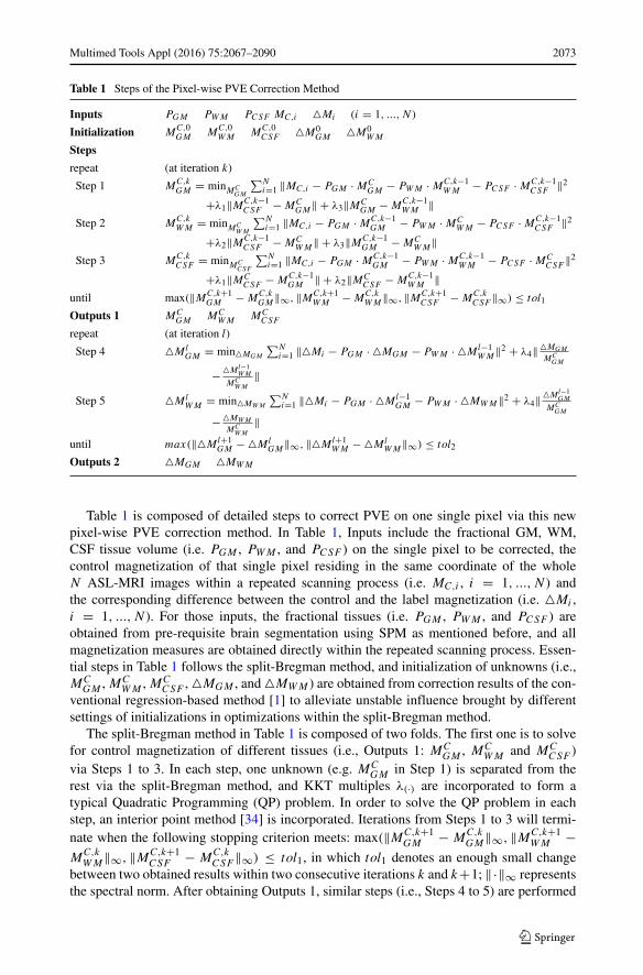
Table 1 is composed of detailed steps to correct PVE on one single pixel via this newpixel-wise PVE correction method. In Table 1, Inputs include the fractional GM, WM,CSF tissue volume (i.e. PGM , PWM , and PCSF ) on the single pixel to be corrected, thecontrol magnetization of that single pixel residing in the same coordinate of the wholeN ASL-MRI images within a repeated scanning process (i.e. MC,i , i = 1, ..., N ) andthe corresponding difference between the control and the label magnetization (i.e. Mi ,i = 1, ..., N ). For those inputs, the fractional tissues (i.e. PGM , PWM , and PCSF ) areobtained from pre-requisite brain segmentation using SPM as mentioned before, and allmagnetization measures are obtained directly within the repeated scanning process. Essen-tial steps in Table 1 follows the split-Bregman method, and initialization of unknowns (i.e.,MC

GM , MCWM , MC

CSF , MGM , and MWM ) are obtained from correction results of the con-ventional regression-based method [1] to alleviate unstable influence brought by differentsettings of initializations in optimizations within the split-Bregman method.

The split-Bregman method in Table 1 is composed of two folds. The first one is to solvefor control magnetization of different tissues (i.e., Outputs 1: MC

GM , MCWM and MC

CSF )via Steps 1 to 3. In each step, one unknown (e.g. MC

GM in Step 1) is separated from therest via the split-Bregman method, and KKT multiples λ(·) are incorporated to form atypical Quadratic Programming (QP) problem. In order to solve the QP problem in eachstep, an interior point method [34] is incorporated. Iterations from Steps 1 to 3 will termi-nate when the following stopping criterion meets: max(‖MC,k+1

GM − MC,kGM‖∞, ‖MC,k+1

WM −M

C,kWM‖∞, ‖MC,k+1

CSF − MC,kCSF ‖∞) ≤ tol1, in which tol1 denotes an enough small change

between two obtained results within two consecutive iterations k and k+1; ‖·‖∞ representsthe spectral norm. After obtaining Outputs 1, similar steps (i.e., Steps 4 to 5) are performed


to calculateMGM andMWM for Outputs 2, following the split-Bregman method as well.After fulfilling all these steps, outcomes obtained from both Outputs 1 and 2 comprise PVEcorrection results obtained by the new pixel-wise PVE correction method. The 2nd row ofFig. 2 demonstrates corresponding correction results obtained by the new method on thesame patient. It can be observed that, problems of blurring and brain details loss which existin the 1st row obtained by the conventional regression-based method can be tackled well.

Although the new method is more sophisticated than the conventional regression-basedmethod and requires more computational time, parallel computing techniques can be incor-porated to improve its efficiency. The merit of the new method in practical implementationis that, PVE correction on each individual pixel only incorporates information obtainedfrom itself, thus PVE corrections on different pixels are totally independent (which is notlike the compared conventional method with neighboring pixels incorporated). Therefore,parallel computing can be carried out with the aid of multi-core & multi-thread processorsfor efficiency boosting in the implementation of the new method. In this study, the averagecomputation time of PVE correction on one patient using the newmethod with parallel com-puting techniques is less than 2 mins using an Intel Core i7-3770 CPU (with 4 cores and 8threads). Thus, the new PVE correction method can effectively handle existing problems ofblurring and brain details loss commonly seen in conventional PVE correction methods, aswell as efficiently accomplish the PVE correction task within an acceptable response time.

3 A novel dementia disease prediction method on corrected ASL-MRI via ranking

After PVE correction on ASL-MRI is conducted, the next critical step is to predict thedementia disease severity of patients based on their ASL-MRI after PVE correction. Con-ventional dementia studies often aim to differentiate patients of various dementia diseaseprogressions, including AD, MCI and Non Cognitive Impairment (NCI) [4, 20, 31, 32, 35].Hence, dementia disease prediction in those conventional studies is often considered aseither a classification or a regression problem, and popular pattern recognition tools suchas SVM and linear/non-linear regressions are often employed [20, 32, 35]. In this section, anovel dementia disease prediction method from a new ranking perspective is presented.

Generally speaking, ranking aims to sort a list of objects according to a system of rat-ing or a record of performance. The intuition to formulate dementia disease prediction viaranking in this study is elaborated as follows. From the conventional classification perspec-tive, such a disease prediction task can be realized by classifying ungraded ASL-MRI intovarious dementia progression stages (i.e., classes), and their disease severity can be sug-gested therein [20, 32, 35]. From the conventional regression perspective, such a diseaseprediction task can be realized within a regression procedure, and disease severities of undi-agnosed patients can be revealed by outcomes of the regression process (i.e., often in termsof real numbers). For both classification and regression methods, ASL-MRI images withclinicians’ diagnosis results are often utilized in their training processes for tuning unknownparameters in either classifiers or regressors, but none of these images will be explicitlyemployed in the subsequent yet important phase, the disease prediction process. Therefore,a typical classification or regression procedure does not comply well with conventionalclinical decision support techniques (e.g., case-based reasoning), in which new cases areto be diagnosed with reference to other previously diagnosed cases. It is known that, sucha case-based reasoning strategy is often relied in real-life clinical diagnosis, and clinicianscan improve their decisions or even gain confidence when referring to previously diagnosedcases. Hence, it inspires us to propose a new dementia disease severity prediction method,


which can explicitly incorporate those previously diagnosed cases in the interpolation ofnew undiagnosed cases, following the introduced conventional clinical decision-makingprocess.

In this study, the disease severity prediction problem is originally considered as a rankingprocess following the above intuition, and ranking can provide a better fit to the predictiontask compared with conventional classification or regression manners. The flowchart of thenew “prediction via ranking” method is illustrated in Fig. 3. The main idea is to sort ASL-MRI into a ranked images list, according to the dementia disease severity depicted in alllisted ASL-MRI images. The disease severity of a new undiagnosed ASL-MRI can then beinterpolated using its neighboring diagnosed ASL-MRI in the ranked list (i.e., Fig. 3). Inorder to achieve such a ranked images list, a ranking function needs to be determined, sothat ASL-MRI images can be sorted into a ranked list based on the ranking function. In thissection, a novel learning method inspired by a conventional position-based ranking evalua-tion measure, the Normalized Discounted Cumulative Gain (NDCG) [15], is introduced tofulfill the ranking function learning task.

The explicit form of NDCG is generally described as below:

NDCG = N−1M × DCG = N−1

M

∑

x∈χ

2r(x) − 1

log2(1 + π(x))(6)

where, x is an ASL-MRI image and χ denotes the set of ASL-MRI images to be ranked;r(x) and π(x) are the annotated dementia disease severity by clinicians (i.e. often in theform of integer grades) and the position of image x within the ranked image list, respec-tively; NM is a normalization term denoting the maximum of DCG, which can be obtainedwhen all images are sorted in a perfect order of decreasing severity of dementia dis-ease. Therefore, the range of NDCG is within [0, 1], where the lower bound and upperbound denote a perfect increasing severity order and a perfect decreasing severity order,respectively.

In order to learn a ranking function based on (6), an optimization process needs to be con-ducted. Unfortunately, optimization cannot be directly applied on (6) for learning ranking

Fig. 3 Flowchart of the “prediction via ranking” method


functions, as NDCG itself is neither continuous nor differentiable in terms of the discreteposition term π(x). Thus, position π(x) needs to be revised and is first approximated asfollows:

π(x) 1 +∑

y =x,y∈χ

sign(sy − sx) = 1 +∑

y =x,y∈χ

sign(f (y) − f (x)

)(7)

where, x represents a d-dimensional feature vector extracted from the ASL-MRI image x;sx is the score of image x calculated from the ranking function f (x), which is of a linearform in this study (i.e. f (x) =< θ, x >, where <, > denotes an inner product between θ

and x. Hence, θ is also a d-dimensional vector and there are d unknown parameters in it tobe learned). sign(sy − sx) is an signum function, whose value is positive when sy ≥ sx andnegative otherwise. The reason to revise position π(x) as (7) is as follows. When the scoreof image x is smaller than that of image y (i.e. sx < sy), sign(sy − sx) becomes positive andπ(x) becomes larger due to (7), which matches the fact that images reflecting lighter diseaseseverity (i.e., indicated by smaller score sx) should be ranked in the rear of a ranked imagelist (i.e. indicated by a larger value of position π(x)), in a demanded descending order ofdisease severity.

Moreover, step transition characteristics of the signum function in (7) makes directionoptimization on (6) still infeasible to be implemented for learning the ranking function f (x).Thus, the signum function in (7) can be further approximated using sign(ζ ) ζ√

ζ 2+α2,

where ζ denotes the variable of the signum function, and α controls the sharpness of theapproximated function towards sign(ζ ). It is shown in Fig. 4 that, the less α becomes,

−10 −5 0 5 10−1

−0.8

−0.6

−0.4

−0.2

0

0.2

0.4

0.6

0.8

1

signum function

α = 0.1

α = 0.5

α = 1

Fig. 4 An illustration of approximating signum function with different α


the more similar it turns towards the signum function. In this way, a new continuousapproximated position π ′(x) can be described as:

π ′(x) 1 +∑

y =x,y∈χ

sign(sy − sx) = 1 +∑

y =x,y∈χ

sign(syx) = 1

+∑

y =x,y∈χ

syx√s2yx + α2

, syx = sy − sx (8)

In this way, a new continuous and differentiable approximation towards NDCG(i.e., denoted as “C-NDCG” in this study) can be explicitly depicted as:

C-NDCG(x) = N−1M

∑

x∈χ

2r(x) − 1

log2(2 + ∑

y =x,y∈χsyx√

s2yx+α2

) (9)

A corresponding algorithm to directly optimize C-NDCG via a gradient method for rank-ing functions learning is listed in Table 2. The critical step here is to calculate the gradient

of C-NDCG with respect to the learned parameter θ(i.e., ∂C-NDCG(x)

∂θ

)in Steps T4&T5 of

Table 2 Steps of ranking functions learning on C-NDCG

Inputs 1. ASL-MRI images for training: x ∈ χ2. ASL-MRI images for validation: xv ∈ χv3. Number of Iterations: T

4. Learning rate: η

TrainingT1. Initialize parameter θ of the ranking function f (x) as θ0

T2. For t = 1 to T

T3. Set θ = θt−1

T4. Feed x ∈ χ to (10) to calculate the gradientT5. Update θ via gradient ascent: θ = θ + η · ∂C-NDCG(x)

∂θ

T6. Set θt = θ

T7. End for T2

Training Validation T learned ranking functions f (x) with T corresponding learned parameters θ

V1. For j = 1 to T

V2. Feed j th learned ranking function fj (x) to xv ∈ χv to rank validation images

V3. Calculate its corresponding NDCG value using (6)

V4. End for V1

V5. Determine fopt (x) as the one with the highest NDCG value

Outputs Optimal learned ranking function: fopt (x)


Table 2. Detailed derivation is elaborated in the Appendix of the paper. The gradient can becomputed as:

∂C-NDCG(x)

∂θ= N−1

M

∑

x∈χ

(− 2r(x) − 1

log22(1 + π ′(x))· 1

(1 + π ′(x)) ln 2

)

×

⎛

⎜⎜⎝∑

y =x,y∈χ

α2

(s2yx + α2

) 32

·(

∂f (y)

∂θ− ∂f (x)

∂θ

)⎞

⎟⎟⎠ (10)

Since the local optimizer of a gradient method cannot always guarantee the global opti-mal solution, we run T iterations of ranking functions learning θt initialized by previouslylearned θ(t−1), where t denotes the t-th iteration. Hence, after conducting the training phasein Table 2, there are T ranking functions learned with their corresponding learned θ . Then,a validation phase is incorporated afterwards to select an optimal ranking function fopt (x)

from those T candidates, as the one with the highest NDCG value after applying all T

learned ranking functions obtained from the training phase to rank the validation set ofimages (i.e., calculated using (6)).

In the testing phase, an undiagnosed ASL-MRI image x is then sorted together withother diagnosed images with clinicians’ annotated grades indicating their disease severi-ties into a ranked image list using fopt (x). Hence, graded information (of those diagnosedcases) is explicitly utilized, which mimics the conventional case-based reasoning procedure.Grade gxi

of the ASL-MRI image x located at position i of the ranked images list can thenbe interpolated using both calculated scores from itself (sxi

) and its neighboring images(sxi−1 , sxi+1 ) as well as their annotated grades (gxi−1 and gxi+1 ), which are known diagno-sis results to clinicians. The grade gxi

of an undiagnosed ASL-MRI image x can then beexplicitly described using the following piecewise function:

gxi=

⎧⎪⎪⎨

⎪⎪⎩

gxi+1 if gxi+1 = gxi−1

gxi+1 + sxi−sxi+1

sxi−1−sxi+1× (gxi−1 − gxi+1) if gxi−1 > gxi+1

gxi−1 + sxi−1−sxi

sxi−1−sxi+1× (gxi+1 − gxi−1) if gxi−1 < gxi+1

(11)

where, sxi= fopt (xi ), sxi−1 = fopt ( ˆxi−1), and sxi+1 = fopt ( ˆxi+1). It can be easily perceived

that, when two neighboring ranked images are of the same disease severity (i.e., gxi+1 =gxi−1 ), the undiagnosed image should share the same severity as them in the ranked imageslist; when two neighboring ranked images are of different disease severities, the severity ofthe undiagnosed image is to be determined by both results of the learned ranking function(i.e., scores) and previously annotated information (i.e., grades), which complies well withthe conventional case-based reasoning procedure.

4 Experiments and analysis

4.1 Data description and pre-processings

In order to demonstrate the superiority of the newly proposed dementia diagnosis strategy,clinical data obtained from 350 real patients, including 110 AD patients, 120 MCI patientsand 120 NCI patients (as normal controls) acquired in the affiliated hospital of NanchangUniversity, is utilized. Informed consent is obtained from all patients for research pur-pose. The averaged age of these patients is 70.56 ± 7.20 years old. In ASL-MRI images


acquisition, A SIEMENS 3T TIM Trio MR scanner is utilized and 23 ASL-MRI imagesare acquired consecutively for each patient to improve the SNR of ASL within a repeatedscanning process (i.e., N =23 in (4) & (5) and relevant Eqs in Table 1). Other acquisitionparameters include: labeling duration = 1500 ms, post-labeling delay = 1500ms, TR/TE =4000/9.1ms, ASL voxel size = 3 × 3 × 5mm3. In PVE correction, pre-defined parametersinclude:λ1 = λ2 = λ3 = 0.1, λ4 = 0.01, tol1 = 10, tol2 = 0.5, the adopted neighbor sizeis 9× 9 when implementing the regression-based PVE correction method for initializationsin Table 1. High-resolution MPRAGE (i.e., which is short for Magnetization Prepared RapidAcquisition Gradient Echo) T1-weighted MRI images [2] are also acquired for all patientssimultaneously in their scannings. After MPRAGE and ASL-MRI images acquisition, brainextraction and motion correction are applied on acquired MPRAGE and ASL-MRI images.The MPRAGE image of every patient is then segmented into GM/WM/CSF componentswith their probability maps PGM , PWM , and PCSF generated for inputs in Table 1, usingthe SPM toolbox [29]. The above obtained maps are then co-registered towards their corre-sponding ASL-MRI images after motion correction for every patient using the FSL toolbox[7].

Experiments in this study are divided into two aspects. The first is to incorporate allpatients’ ASL-MRI images to demonstrate the superiority of the new pixel-wise PVE cor-rection method (i.e., Step 1 of the newly introduced strategy), in comparison with otherconventional PVE correction methods (Section 4.2). The second is to apply the new “predic-tion via ranking” method on ASL-MRI after PVE correction to diagnose dementia disease(i.e., Step 2 of the newly introduced strategy), in comparison with several popular pat-tern recognition tools to reveal the superiority of the new ranking method (Section 4.3).Comprehensive statistical analysis is performed in all experiments.

4.2 Experiments and analysis on PVE correction

As introduced in Section 1, ASL-MRI images suffering from PVE will often result inunder-estimated CBF, and superior PVE correction methods will often improve CBF afterPVE correction better. The newly proposed pixel-wise PVE correction method (denotedas “New”) is compared with the conventional regression-based PVE correction method(denoted as “RB”), regarding calculated CBF from their corrected ASL-MRI results. Forcompared RBmethods, different sizes of neighbors are implemented in experiments, includ-ing sizes of 9 × 9 (i.e., to illustrate a small size of neighborhood), and 15 × 15 (i.e.,to illustrate a large size of neighborhood). They are denoted as “RB-9” and “RB-15”,respectively.

Figure 5 displays PVE correction results of an AD patient obtained by all compared PVEcorrection methods. In this figure, each row represents correction results obtained by onemethod. For columns of Fig. 5, the first column depicts the solved control magnetizationin GM

(i.e. MC

GM

), the second column displays the solved control magnetization in WM(

i.e. MCWM

), the third column demonstrates the solved control magnetization in CSF (i.e.

MCCSF ), and the forth column illustrates histograms of subject-wise averaged ASL sig-

nal MGM

MCGM

(red) and MWM

MCWM

(blue), as well as the calculated voxel-wise ratio of GM flow

towards WM flow annotated on tops of histograms. It can be easily observed that, blurringand brain details loss in correction results of “New” can be greatly improved. Also, the ratioof GM flow to WM flow obtained by “New” is 2.0314, which complies well with clinicalliteratures [17, 26] compared with other methods (e.g., ratio results of “RB-9” and “RB-15”are 1.6853, and 1.7601, respectively in Fig. 5, which are significantly smaller and do not


MCGM

0

500

1000

1500

2000

MCWM

0

500

1000

1500

2000

MCSF

0

500

1000

1500

2000

0 0.005 0.01 0.015 0.020

200

400

600

800

1000

1200

1400

1600

1800

2000ratio GM/WM =2.0314

WMGM

MCGM

0

500

1000

1500

2000

MCWM

0

500

1000

1500

2000

MCSF

0

500

1000

1500

2000

0 0.005 0.01 0.015 0.020

200

400

600

800

1000

1200

1400

1600

1800

2000ratio GM/WM =1.6853

WMGM

MCGM

0

500

1000

1500

2000

MCWM

0

500

1000

1500

2000

MCSF

0

500

1000

1500

2000

0 0.005 0.01 0.015 0.020

200

400

600

800

1000

1200

1400

1600

1800

2000ratio GM/WM =1.7601

WMGM

MCGM

0

500

1000

1500

2000

MCWM

0

500

1000

1500

2000

MCSF

0

500

1000

1500

2000

0 0.005 0.01 0.015 0.020

200

400

600

800

1000

1200

1400

1600

1800

2000ratio GM/WM =2.0314

WMGM

MCGM

0

500

1000

1500

2000

MCWM

0

500

1000

1500

2000

MCSF

0

500

1000

1500

2000

0 0.005 0.01 0.015 0.020

200

400

600

800

1000

1200

1400

1600

1800

2000ratio GM/WM =1.6853

WMGM

MCGM

0

500

1000

1500

2000

MCWM

0

500

1000

1500

2000

MCSF

0

500

1000

1500

2000

0 0.005 0.01 0.015 0.020

200

400

600

800

1000

1200

1400

1600

1800

2000ratio GM/WM =1.7601

WMGM

MCGM

0

500

1000

1500

2000

MCWM

0

500

1000

1500

2000

MCSF

0

500

1000

1500

2000

0 0.005 0.01 0.015 0.020

200

400

600

800

1000

1200

1400

1600

1800

2000ratio GM/WM =2.0314

WMGM

MCGM

0

500

1000

1500

2000

MCWM

0

500

1000

1500

2000

MCSF

0

500

1000

1500

2000

0 0.005 0.01 0.015 0.020

200

400

600

800

1000

1200

1400

1600

1800

2000ratio GM/WM =1.6853

WMGM

MCGM

0

500

1000

1500

2000

MCWM

0

500

1000

1500

2000

MCSF

0

500

1000

1500

2000

0 0.005 0.01 0.015 0.020

200

400

600

800

1000

1200

1400

1600

1800

2000ratio GM/WM =1.7601

WMGM

Fig. 5 PVE correction results on an AD patient obtained by different methods (1st row: New; 2nd row:RB-9; 3rd row: RB-15)

comply well with clinical literatures). Similar results can be observed in all 350 patients aswell. After calculating CBF of all patients based on correction results obtained from all PVEcorrection methods, a box-and-whisker plot summarizing CBF of all patients is illustratedin Fig. 6. In each box, a horizontal line is drawn across the box at the median of CBF, whilethe upper- and lower-quartiles of CBF are depicted as lines above and below the median. Avertical dashed line is drawn up from the upper-quartile and down from the lower-quartileto their most extreme data points, which are within a distance of 1.5 Inter-Quartile Range(IQR) [28]. Each data point beyond ends of the vertical line is marked via a plus sign. It can

40

50

60

70

80

90

100

110

New RB−9 RB−15

CB

F

Fig. 6 Box plot of CBF obtained by all compared PVE correction methods


be observed that, the box of “New” is significantly higher than those of others, which indi-cates that the under-estimated CBF in original ASL-MRI images can be improved better bythe new pixel-wise correction method.

In order to reveal the superiority of “New” in PVE correction from the statistical pointof view, a statistical test made up of one-way Analysis Of Variance (ANOVA) followed bypost-hoc multiple comparison tests [28] is further utilized for statistical analysis on all CBFresults obtained by all compared PVE correction methods on all patients data. ANOVA isa popular correction of models analyzing the difference between diverse group means andtheir associated variations in statistics [28]. In one-way ANOVA, CBF results obtained fromall methods are compared to test a hypothesis (H0) that “CBF means of various methodsare equivalent”, against the general alternative that these means cannot be all the same. P-value is used here as an indicator to reveal whether H0 holds or not. In this study, p-valuescalculated from all CBF results are nearly 0, which is a strong indication that all thesemethods cannot share the same CBF means. Therefore, the next step is to conduct moredetailed paired comparisons. The reason to do so is because that, the alternative against H0is too general. Information about which method is superior from the statistical perspectivecannot be perceived by one-way ANOVA alone. There are two kinds of evaluation afterapplying multiple comparison tests on calculated CBF of all methods, and quantitative eval-uation results are shown in Table 3. For the two kinds of evaluation, one is estimated CBFmean difference, which is a single-value estimator of CBF mean difference. Another is a95 % Confidence Interval (CI). In statistics, a CI is a special form of interval estimator fora parameter (i.e. CBF mean difference in this experiment). Generally speaking, instead ofestimating the parameter by a single value, CI is capable to provide an interval estimationwhich is likely to include the estimated parameter within a specified interval. To be spe-cific, “New” is 4.3904 higher than “RB-9”. The CBF mean difference (i.e., using “New”minus “RB-9”) is likely to fall within a 95 % CI [2.2873, 6.4935]. Since the upper and lowerbounds of the CI are both positive, it gives a strong indication (> 95 %) that the CBF meandifference should be positive. Thus, “New” is superior to “RB-9” in terms of CBF from sta-tistical point of view. For comparisons between “New” and “RB-15”, a similar conclusioncan be drawn from Table 3. To sum up, based on the above statistical analysis, the pixel-wisePVE correction method in the newly introduced dementia diagnosis strategy outperformscompared conventional regression-based methods, from the statistical perspective.

4.3 Experiments and analysis of disease severity prediction

After PVE correction has been fulfilled, the next critical step is to conduct dementia dis-ease severity prediction. In this section, the “prediction via ranking” method (denoted as“Ranking”) is evaluated for its capability of dementia disease prediction, based on ASL-MRI after PVE correction. Its pre-defined parameters are set as T = 200 and η = 0.01 in

Table 3 Multiple comparison test of obtained CBF based on Corrected ASL-MRI from all PVE correctionmethods

Method I Method II CBF Mean Difference (I-II) a 95 % Confidence Interval

New RB-9 4.3904 [2.2873, 6.4935]

New RB-15 2.5758 [0.4727, 4.6789]

RB-9 RB-15 −1.8146 [-3.9177, 0.2885]


Table 2 through trial-and-error for optimal performance; α in (8) controlling the sharpnessof the approximated function towards the signum function is set as 0.1. Mean ASL signalcalculated from the segmented left & right hippocampus, the left & right parahippocampalgyrus, the left & right putamen, and the left & right thalamus (i.e. the above tissue segmen-tation is realized via IBA-SPM [14]) is utilized to construct a 8-dimensional feature vectorx in (7) for each patient. Popular pattern recognition tools widely utilized in conventionaldementia diagnosis studies, including support vector machine (denoted as “SVM” as a clas-sification tool), support vector regression (denoted as “SVR” as a non-linear regressiontool) and linear regression (denoted as “LR”), are implemented in this experiment based onASL-MRI images of all patients after PVE correction, for dementia diagnosis. Since learn-ing is incorporated in “Ranking”, parameters of other methods are also learned for the sakeof fairness. For “SVM” and “SVR”, Gaussian Radial Basis Function (RBF) are adopted askernels; Gaussian widths are learned via the popular radius/margin bound algorithm [18],and SVM-light toolbox [16] is utilized for their implementations. For “LR” and “Ranking”,disease severities of AD, MCI and NCI are labeled as 1, 2 and 3 respectively. Regressioncoefficients in “LR” are determined via labels and regressors (i.e., the 8-dimensional featurevector) of the training data.

The whole dataset of 350 patients is equally divided into 5 subsets to conduct a 5-foldcross validation for statistical evaluation. In each subset, patients with different dementiadisease severities are roughly equivalent (i.e., 22 AD/ 24 MCI/ 24 NCI in each subset).Since there are training, validation and testing phases in the “Ranking” method and thenumber of subsets utilized in them are 3, 1 and 1 individually in each trial of the 5-fold crossvalidation, the total number of trials in the whole 5-fold cross validation isC3

5 ·C12 ·C1

1 = 20,

where C()(∗) denotes the number of combinations of objects from a set of ∗ objects. For

other compared methods without the validation phase (i.e., “SVM”, “SVR” and “LR”), allnon-testing subsets (i.e., training+validation subsets) are utilized for parameters learningin each trial. In order to perceive comprehensive understandings of the newly proposeddementia diagnosis strategy, all compared disease severity prediction methods are tested onall corrected ASL-MRI obtained by all compared PVE correction methods in Sections 4.2,and the combination of PVE correction and disease prediction methods producing the bestperformance in dementia diagnosis can be suggested therein.

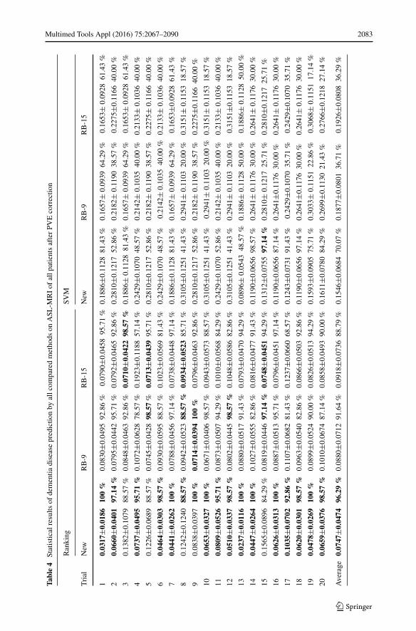
Statistical results of dementia disease prediction obtained by all combinations of PVEcorrection methods and disease severity prediction methods are elaborated in Table 4. Eachentry in Table 4 contains the mean±standard deviation of the difference between predicteddisease severity (i.e., grade) and its ground truth annotated by our senior clinicians deter-mined by consensus, as well as the prediction accuracy (i.e., in percentage) in which onepredicted case is considered to be accurate if the difference between its prediction andground truth is less than 0.3 (i.e., suggested by our senior clinicians based on clinical evi-dence). The least prediction error and the highest prediction accuracy in each trial arehighlighted. It can be observed from Table 4 that, the combination of the pixel-wise PVEcorrection method (“New”) and the “prediction via ranking” method (“Ranking”) achievesthe highest prediction accuracy and the least prediction error in most trials (i.e. 17 out of20 trials with the highest prediction accuracy, and 15 out of 20 trials with the least predic-tion error). We investigated trials that the newly proposed ranking method cannot performthe best, and found that characteristics between different patients vary more in those tri-als. Since ranking is more generative than conventional classification, it is more convenientfor classification models to tackle those more discriminant cases. However, based on allstatistics, the generative ranking method still achieves the most satisfactory outcomes. To


Table4

Statisticalresults

ofdementia

diseasepredictio

nby

allcom

paredmethods

onASL

-MRIof

allp

atientsafterPV

Ecorrectio

n

Ranking

SVM

Trial

New

RB-9

RB-15

New

RB-9

RB-15

10.0317

±0.0186

100%

0.0830

±0.0495

92.86%

0.0790

±0.0458

95.71%

0.1886

±0.1128

81.43%

0.1657

±0.0939

64.29%

0.1653

±0.0928

61.43%

20.0660

±0.0401

97.14%

0.0795

±0.0442

95.71%

0.0792

±0.0465

92.86%

0.2810

±0.1217

52.86%

0.2182

±0.1190

38.57%

0.2275

±0.1166

40.00%

30.1382

±0.1079

88.57%

0.0848

±0.0463

92.86%

0.0710

±0.0422

98.57%

0.1886

±0.1128

81.43%

0.1657

±0.0939

64.29%

0.1653

±0.0928

61.43%

40.0737

±0.0495

95.71%

0.1072

±0.0628

78.57%

0.1923

±0.1188

57.14%

0.2429

±0.1070

48.57%

0.2142

±0.1035

40.00%

0.2133

±0.1036

40.00%

50.1226

±0.0689

88.57%

0.0745

±0.0428

98.57%

0.0713

±0.0439

95.71%

0.2810

±0.1217

52.86%

0.2182

±0.1190

38.57%

0.2275

±0.1166

40.00%

60.0464

±0.0303

98.57%

0.0930

±0.0595

88.57%

0.1023

±0.0569

81.43%

0.2429

±0.1070

48.57%

0.2142

±0.1035

40.00%

0.2133

±0.1036

40.00%

70.0441

±0.0262

100%

0.0788

±0.0456

97.14%

0.0738

±0.0448

97.14%

0.1886

±0.1128

81.43%

0.1657

±0.0939

64.29%

0.1653

±0.0928

61.43%

80.1242

±0.1240

88.57%

0.0942

±0.0523

88.57%

0.0934

±0.0523

85.71%

0.3105

±0.1251

41.43%

0.2941

±0.1103

20.00%

0.3151

±0.1153

18.57%

90.0838

±0.0397

100%

0.0714

±0.0394

100%

0.0796

±0.0463

92.86%

0.2810

±0.1217

52.86%

0.2182

±0.1190

38.57%

0.2275

±0.1166

40.00%

100.0653

±0.0327

100%

0.0671

±0.0406

98.57%

0.0943

±0.0573

88.57%

0.3105

±0.1251

41.43%

0.2941

±0.1103

20.00%

0.3151

±0.1153

18.57%

110.0809

±0.0526

95.71%

0.0873

±0.0507

94.29%

0.1010

±0.0568

84.29%

0.2429

±0.1070

52.86%

0.2142

±0.1035

40.00%

0.2133

±0.1036

40.00%

120.0510

±0.0337

98.57%

0.0802

±0.0445

98.57%

0.1048

±0.0586

82.86%

0.3105

±0.1251

41.43%

0.2941

±0.1103

20.00%

0.3151

±0.1153

18.57%

130.0237

±0.0116

100%

0.0880

±0.0517

91.43%

0.0793

±0.0470

94.29%

0.0896

±0.0543

48.57%

0.1886

±0.1128

50.00%

0.1886

±0.1128

50.00%

140.0447

±0.0264

100%

0.1027

±0.0555

82.86%

0.0816

±0.0477

91.43%

0.1190

±0.0656

98.57%

0.2641

±0.1176

30.00%

0.2641

±0.1176

30.00%

150.1565

±0.0896

84.29%

0.0819

±0.0446

97.14%

0.0748

±0.0451

94.29%

0.1312

±0.0755

97.14%

0.2810

±0.1217

25.71%

0.2810

±0.1217

25.71%

160.0626

±0.0313

100%

0.0887

±0.0513

95.71%

0.0796

±0.0451

97.14%

0.1190

±0.0656

87.14%

0.2641

±0.1176

30.00%

0.2641

±0.1176

30.00%

170.1035

±0.0702

92.86%

0.1107

±0.0682

81.43%

0.1237

±0.0660

68.57%

0.1243

±0.0731

91.43%

0.2429

±0.1070

35.71%

0.2429

±0.1070

35.71%

180.0620

±0.0301

98.57%

0.0963

±0.0540

82.86%

0.0866

±0.0503

92.86%

0.1190

±0.0656

97.14%

0.2641

±0.1176

30.00%

0.2641

±0.1176

30.00%

190.0478

±0.0269

100%

0.0899

±0.0524

90.00%

0.0826

±0.0513

94.29%

0.1593

±0.0905

75.71%

0.3033

±0.1151

22.86%

0.3068

±0.1151

17.14%

200.0659

±0.0376

98.57%

0.1010

±0.0674

87.14%

0.0858

±0.0493

90.00%

0.1611

±0.0780

84.29%

0.2699

±0.1130

21.43%

0.2766

±0.1218

27.14%

Average

0.0747

±0.0474

96.29%

0.0880

±0.0712

91.64%

0.0918

±0.0736

88.79%

0.1546

±0.0684

70.07%

0.1877

±0.0801

36.71%

0.1926

±0.0808

36.29%


Table4

(contin

ued)

SVR

LR

Trial

New

RB-9

RB-15

New

RB-9

RB-15

10.1380

±0.0783

91.43%

0.1848

±0.1078

55.71%

0.1698

±0.1125

64.29%

0.2999

±0.2237

32.86%

0.3619

±0.2610

31.43%

0.3291

±0.2399

31.43%

20.1916

±0.0969

75.71%

0.2120

±0.1018

35.71%

0.2637

±0.1207

31.43%

0.2205

±0.2481

37.14%

0.1458

±0.2390

18.57%

0.1770

±0.2436

20.00%

30.1723

±0.1081

77.14%

0.1991

±0.1208

52.86%

0.2081

±0.1345

57.14%

0.2999

±0.2237

32.86%

0.3619

±0.0939

31.43%

0.3291

±0.2399

31.43%

40.2194

±0.1141

68.57%

0.2951

±0.1298

30.00%

0.2647

±0.1298

37.14%

0.1770

±0.0742

58.57%

0.1351

±0.2579

31.43%

0.1254

±0.2036

37.14%

50.1957

±0.0979

74.29%

0.2077

±0.1031

38.57%

0.2529

±0.1247

37.14%

0.2205

±0.2481

37.14%

0.1458

±0.2390

18.57%

0.1770

±0.2436

20.00%

60.2248

±0.1137

65.71%

0.2524

±0.1303

41.43%

0.2871

±0.1393

35.71%

0.1770

±0.1742

57.14%

0.1351

±0.2579

31.43%

0.1254

±0.2036

37.14%

70.1387

±0.1125

90.00%

0.1653

±0.1079

62.86%

0.2012

±0.1291

51.43%

0.2999

±0.2237

32.86%

0.3619

±0.2610

31.43%

0.3291

±0.2399

31.43%

80.1716

±0.0934

75.71%

0.3048

±0.1258

25.71%

0.2620

±0.1203

31.43%

0.1470

±0.1881

60.00%

0.1393

±0.1713

51.43%

0.1108

±0.1595

51.43%

90.1987

±0.0998

74.29%

0.2143

±0.1082

42.86%

0.2570

±0.1353

40.00%

0.2205

±0.2481

37.14%

0.1458

±0.2390

18.57%

0.1770

±0.2436

20.00%

100.1686

±0.0919

77.14%

0.2904

±0.1290

31.43%

0.2782

±0.1190

28.57%

0.1470

±0.1881

60.00%

0.1393

±0.1713

51.43%

0.1108

±0.1595

51.43%

110.2256

±0.1152

65.71%

0.3038

±0.1332

28.57%

0.2686

±0.1327

35.71%

0.1770

±0.1742

57.14%

0.1351

±0.2579

31.43%

0.1254

±0.2036

37.14%

120.1684

±0.0922

77.14%

0.3050

±0.1255

25.71%

0.2830

±0.1151

24.29%

0.1470

±0.1881

60.00%

0.1393

±0.1713

51.43%

0.1108

±0.1595

51.43%

130.1997

±0.1223

75.71%

0.1883

±0.1101

52.86%

0.1686

±0.1051

58.57%

0.2999

±0.2237

32.86%

0.3619

±0.2610

31.43%

0.3291

±0.2399

31.43%

140.2384

±0.1111

64.29%

0.2368

±0.1093

31.43%

0.2579

±0.1097

30.00%

0.2044

±0.2527

45.71%

0.1024

±0.1991

48.57%

0.1341

±0.1815

52.86%

150.1975

±0.1002

74.29%

0.2327

±0.1053

32.86%

0.2656

±0.1182

30.00%

0.2205

±0.2481

37.14%

0.1458

±0.2390

28.57%

0.1770

±0.2436

30.00%

160.2273

±0.1125

68.57%

0.2304

±0.1084

32.86%

0.2572

±0.1093

28.57%

0.2044

±0.252745.71%

0.1024

±0.1991

48.57%

0.1341

±0.1815

52.86%

170.2196

±0.1121

67.14%

0.2766

±0.1320

34.29%

0.2983

±0.1318

24.29%

0.1770

±0.1742

47.14%

0.1351

±0.2579

31.43%

0.1254

±0.2036

37.14%

180.2273

±0.1123

68.57%

0.2394

±0.1092

27.14%

0.2685

±0.1087

24.29%

0.2044

±0.2527

45.71%

0.1024

±0.1991

48.57%

0.2641

±0.1815

52.86%

190.1679

±0.0921

77.14%

0.2984

±0.1278

30.00%

0.2583

±0.1153

28.57%

0.1470

±0.1881

60.00%

0.1393

±0.1713

51.43%

0.1108

±0.1595

51.43%

200.2305

±0.1116

67.14%

0.2384

±0.1099

31.43%

0.2593

±0.1105

28.57%

0.2044

±0.2527

45.71%

0.1024

±0.1991

48.57%

0.1341

±0.1815

52.86%

Average

0.1461

±0.0744

73.79%

0.1938

±0.0868

37.21%

0.2015

±0.0911

36.36%

0.1698

±0.1174

36.57%

0.2369

±0.1257

26.29%

0.2110

±0.1056

28.57%


be specific, the average prediction accuracy of the newly introduced dementia disease diag-nosis strategy in this study (i.e., “New”+“Rank”) is 96.29 %, and 0.0747 ± 0.0474 as itsmean and standard deviation of prediction errors. The above outcomes are superior to onesof other combinations based on all patients data.

Another interesting thing to notice is that, for one specific prediction method (e.g. “Rank-ing”), corrected ASL-MRI obtained by the pixel-wise correction method (e.g., “New”) canhelp to provide better dementia disease prediction performance than ones obtained by com-pared conventional regression-based methods (i.e., “RB-9” and “RB-15”). For instance, theaveraged prediction accuracy is 96.29 % for “New”+“Ranking”, compared with 91.64 %for “RB-9”+“Ranking” and 88.79 % for “RB-15”+“Ranking”. Similar conclusions can alsobe drawn in each of other disease severity prediction methods (e.g., “SVM”, “SVR” and“LR”) when comparing prediction results based on different PVE correction methods. Allthese observations demonstrate the effectiveness of the pixel-wise PVE correction methodin differentiating patients with various dementia disease severities in both conventionalprediction methods and the newly introduced “prediction via ranking” method. Also, forcorrected ASL-MRI obtained by one specific PVE correction method, the newly introduced“prediction via ranking” method outperforms other conventional prediction methods. Forinstance, based on corrected ASL-MRI obtained by “New”, the dementia diagnosis predic-tion accuracy of “New”+“Ranking”, “New”+“SVM”, “New”+“SVR” and “New”+“LR” are96.29 %, 70.07 %, 73.79 % and 36.57 %, respectively. Thus, the effectiveness of the newlyintroduced “prediction via ranking” method can also be verified.

In Fig. 7, a histogram depicting the distribution of prediction errors obtained by the newlypresented dementia disease diagnosis strategy in this study (i.e., “New”+“Rank”) is illus-trated based on all diagnosis results obtained from the 5-fold cross validation on all patientsdata. The number of testing data in Fig. 7 is 1400 (which equals to 350 × 4, as each testingsubset will be utilized C3

4 × C11 = 4 times brought by different combinations of training

−1 −0.5 0 0.5 10

50

100

150

200

250

300

Prediction Error

Cou

nts

Fig. 7 Histogram of prediction errors obtained by the newly proposed dementia disease diagnosis strategy


−0.05

0

0.05

0.1

0.15

0.2

0.25

0.3

1 2 3 4 5 6 7 8Dimensions of the extracted feature vector from corrected ASL−MRI

Lear

ned

wei

ghts

on

diffe

rent

dim

ensi

ons

Fig. 8 Summary of learned weights on different dimensions of the extracted feature according to outcomesin “New”+“Rank”

and validation subsets in the 5-fold cross validation). It can be observed that, the predictionerror of most cases is within the range [-0.5, 0.5]. In Fig. 8, the distribution of all 8 elementsof the learned θ in the utilized linear ranking function f (x) =< θ, x > of this study is sum-marized based on all learned θ results from the 5-fold cross validation on “New”+“Rank”,where indices 1-8 in Fig. 8 denotes the left & right hippocampus, the left & right parahip-pocampal gyrus, the left & right putamen, and the left & right thalamus sequentially. It canbe observed from Fig. 8 that, all of them have dominant influence on dementia disease diag-nosis (i.e., all medians are within [0.05, 0.15] without much difference), which complieswell with clinical literatures in dementia studies [9, 11, 19].

5 Conclusion

In this study, a new dementia disease diagnosis strategy based on ASL-MRI is proposedfor the first time. There are two steps composed of the whole strategy, including pixel-wisePVE correction and dementia disease severity prediction via ranking. Extensive experimen-tal results and comprehensive statistical analysis demonstrate the superiority of the newdisease diagnosis strategy. Main contributions of this study can be summarized as: 1) A newpixel-wise PVE correction method on ASL-MRI, which is capable to tackle problems ofblurring and brain details loss in correction results commonly seen in conventional PVE cor-rection methods as well as better improve CBF; 2) The first attempt to diagnose dementiadisease based on corrected ASL-MRI from a new ranking perspective. Experimental analy-sis demonstrates the superiority of the newly proposed dementia disease diagnosis strategyover several compared existing methods. Future studies will be continued with more sophis-ticated ranking models investigated for severity prediction of diverse diseases reflected bydifferent modalities of medical images.


Acknowledgments The authors would like to acknowledge national grants 61403182, 61363046,61301194 and 61302121 approved by the National Natural Science Foundation of China, grants20142BBE50023 and 20142BAB217033 approved by the Jiangxi Provincial Department of Science andTechnology, as well as the NWPU grant 3102014JSJ0014 for supporting this study.

Appendix: Derivation of Equation (10)

After applying the chain rule, the gradient of C-NDCG(x) with respect to θ becomes:

∂C-NDCG(x)

∂θ= ∂C-NDCG(x)

∂π ′(x)· ∂π ′(x)

∂θ= N−1

M

∑

x∈χ

∂ 2r(x)−1

log2(1+π ′(x)

)

∂π ′(x)· ∂π ′(x)

∂θ(12)

where, the first term of (12) is derived as follows:

∂ 2r(x)−1

log2(1+π ′(x)

)

∂π ′(x)= − 2r(x) − 1

log22(1 + π ′(x)

) · 1(1 + π ′(x)

)ln 2

(13)

Furthermore, π ′(x) in (13) can be re-written as follows:

π ′(x) 1 +∑

y =x,y∈χ

syx√s2yx + α2

, syx = sy − sx (14)

Apply the chain rule to the second term of (12) after incorporating results in (14):

∂π ′(x)

∂θ= ∂π ′(x)

∂syx

· ∂syx

∂θ

=∑

y =x,y∈χ

√s2yx + α2 − syx · 1

2 · 1√s2yx+α2

· 2syx

s2yx + α2· ∂syx

∂θ

=∑

y =x,y∈χ

s2yx + α2 − syx · syx

(s2yx + α2

) 32

· ∂syx

∂θ

=∑

y =x,y∈χ

α2

(s2yx + α2

) 32

·(

∂f (y)

∂θ− ∂f (x)

∂θ

)(15)

Hence, after substituting derivation results of (13) & (15) into (12), it becomes:

∂C-NDCG(x)

∂θ= N−1

M

∑

x∈χ

(− 2r(x) − 1

log22(1 + π ′(x))· 1

(1 + π ′(x)) ln 2

)

×

⎛

⎜⎜⎝∑

y =x,y∈χ

α2

(s2yx + α2

) 32

·(

∂f (y)

∂θ− ∂f (x)

∂θ

)⎞

⎟⎟⎠ (16)

which is the same as (10).


References

1. Asllani I, Borogovac A, Brown T (2008) Regression algorithm correcting for partial volume effects inarterial spin labeling MRI. Magn Reson Med 60:1362–1371

2. Brant-Zawadzki M, Gillan G, Nitz W (1992) MPRAGE: a three-dimensional, t1-weighted, qradient-echosequence–initial experience in the brain. Radiology 182(3):769–775

3. Brookmeyer R, Johnson E, Ziegler-Graham K, Arrighi M (2007) Forecasting the global burden ofalzheimer’s disease. Alzheimers Dement 3(3):186–191

4. Chen Y, Wolk D, Reddin J, Korczykowski M, Martinez P, Musiek E, Newberg A, Julin P, Arnold S,Greenberg J, Detre J (2011) Voxel-level comparison of arterial spin-labeling perfusion mri and fdg-petin alzheimer disease. Neurology 77(2):1977–1985

5. Du Y, Tsui B, Frey E (2005) Partial volume effect compensation for quantitative brain spect imaging.IEEE Trans Med Imaging 24(8):969–976

6. Erlandsson K, Buvat I, Pretorius H, Thomas B, Hutton B (2012) A review of partial volume correctiontechniques for emission tomography and their applications in neurology, cardiology and oncology. PhysMed Biol 57(21):119–159

7. FMRIB Software Library (FSL) toolbox. http://fsl.fmrib.ox.ac.uk/fsl/fslwiki/8. Folstein M, Folstein S, McHung P (1975) Mini-mental state: a practical method for grading the cognitive

state of patients for the clinician. J Psychiatr Res 12(3):189–1989. Galton C, Patterson K, Graham K, Lambon-Ralph M, Williams G, Antoun N, Sahakian B, Hodges J

(2001) Differing patterns of temporal atrophy in alzheimer’s disease and semantic dementia. Neurology57(2):216–225

10. Golay X, Hendrikse J, Lim T (2004) Perfusion imaging using arterial spin labeling. Top Magn ResonImaging: TMRI 15(1):10–27

11. Gold G, Eniko K, Herrmann F, Canuto A, Hof P, Jean-Pierre M, Constantin B, Giannakopoulos P (2005)Cognitive consequences of thalamic, basal ganglia, and deep white matter lacunes in brain aging anddementia. Stroke 36(6):1184–1188

12. Goldstein T, Osher S (2008) The Split Bregman Method for L1 Regularized Problems. UCLA CAMreport 08–29:1–21

13. Gunn R, Gunn S, Turkheimer F, Aston J, Cunningham V (2002) Positron emission tomography com-partmental models: a basis pursuit strategy for kinetic modeling. J Cereb Blood Flow Metab 22:1425–1439

14. Individual Brain Atlases using Statistical Parametric Mapping (IBA-SPM) Software. http://www.thomaskoenig.ch/Lester/ibaspm.htm

15. Jarvelin K, Kekalainen J (2000) IR Evaluation Methods for Retrieving Highly Relevant Documents. In:Proceedings ACM Special Interest Group Inf Retrieval (SIGIR), pp. 41–48

16. Joachims T SVM light - An Implementation of Support Vector Machine in C. URL http://svmlight.joachims.org

17. Johnson N, Jahng G, Weiner M, Miller B, Chui H, Jagust W, Gorno-Tempini M, Schuff N (2005) Patternof cerebral hypoperfusion in alzheimer disease and mild cognitive impairment measured with arterialspin-labeling mr imaging: initial experience. Radiology 234:851–859

18. Keerthi S (2002) Efficient Tuning of SVM Hyperparameters using Radius/Margin Bound and IterativeAlgorithms. IEEE Trans Neural Netw 13(5):1225–1229

19. Laakso M, Partanen K, Riekkinen P, Lehtovirta M, Helkala E, Hallikainen M, Hanninen T, Vainio P,Soininen H (1996) Hippocampal volumes in alzheimer’s disease, parkinson’s disease with and withoutdementia, and in vascular dementia an mri study. Neurology 46(3):678–681

20. Liu M, Zhang D, Shen D (2012) Ensemble sparse classification of alzheimers disease. NeuroImage60(2):1106–1116

21. Mahendra B (1987) A pathography of dementia. Dementia 1:189–20222. Malpass K, Disease Alzheimer (2012) Arterial Spin-Labeled MRI for Diagnosis and Monitoring of AD.

Nat Rev Neurol 8(3):847–849

http://fsl.fmrib.ox.ac.uk/fsl/fslwiki/

http://www.thomaskoenig.ch/Lester/ibaspm.htm

http://www.thomaskoenig.ch/Lester/ibaspm.htm

http://svmlight.joachims.org

http://svmlight.joachims.org


23. Mioshi E, Dawson K, Mitchell J, Arnold R, Hodges J (2006) The addenbrooke’s cognitive examinationrevised (ace-r): a brief cognitive test battery for dementia screening. Int J Geriatr Psychiatr 21(11):1078–1085

24. Murphy K, Brunberg J, Cohan R (1996) Adverse reactions to gadolinium contrast media: a review of 36cases. Am J Roentgenol 167(4):847–849

25. Musiek E, Chen Y, Korczykowski M, Saboury B, Martinez P, Reddin J, Alavi A, Kimberg D, WolkD, Julin P, Newberg A, Arnold S, Detre J (2012) Direct comparison of fluorodeoxyglucose positronemission tomography and arterial spin labeling magnetic resonance imaging in alzheimer’s disease.Alzheimers Dement 8(1):51–59

26. Parkes L, Rashid W, Chard D, Tofts P (2004) Normal cerebral perfusion measurements using arterialspin labeling: reproducibility, stability, and age and gender effects. Magn Reson Med 51:736–743

27. Partial volume imaging. http://en.wikipedia.org/wiki/Partial volume (imaging)28. Rice J (2007) Mathematical Statistics and Data Dnalysis, second edition. Duxbury Press29. Statistical Parametric Mapping (SPM) toolbox. http://www.fil.ion.ucl.ac.uk/spm/30. United Nations, World Population Prospects. http://www.un.org/esa/population/publications/wpp2006/

WPP2006 Highlights rev.pdf31. Wang Z, Das S, Xie S, Arnold S, Detre J (2013) Arterial Spin Labeled MRI in Prodromal Alzheimer’s

Disease: A Multi-site Study. NeuroImage: Clin 2:630–63632. Wee C, Yap P, Shen D (2013) Prediction of alzheimers disease and mild cognitive impairment using

cortical morphological patterns. Hum Brain Mapp 34(12):3411–342533. World Health Organization, The Top 10 Causes of Death. http://www.who.int/mediacentre/factsheets/

fs310/en/index2.html34. Wright M (2004) The interior-point revolution in optimization: history, recent developments, and lasting

consequences. Bull Am Math Soc 42(39):1–1635. Zhou L, Wang Y, Li Y, Yap P, Shen D (2011) Hierarchical Anatomical Brain Networks for MCI

Prediction: Revisiting Volumetric Measures. PLoS Comput Biol 6(7):e21935

Wei Huang obtained his B.Eng. and M.Eng. from the Harbin Institute of Technology, China in 2004 and2006, respectively. He obtained his Ph.D. from the Nanyang Technological University, Sinagpore in 2011.Before joining the Nanchang University as an Associate Professor, he worked in the University of CaliforniaSan Diego, USA, as well as the Agency for Science Technology and Research, Singapore as Research Staffs.Dr. Huang’s recent research interests mainly include but not limited to medical image processing, patternrecognition, and computer vision.

http://en.wikipedia.org/wiki/Partial_volume_(imaging)

http://www.fil.ion.ucl.ac.uk/spm/

http://www.un.org/esa/population/publications/wpp2006/WPP2006_Highlights_rev.pdf

http://www.un.org/esa/population/publications/wpp2006/WPP2006_Highlights_rev.pdf

http://www.who.int/mediacentre/factsheets/fs310/en/index2.html

http://www.who.int/mediacentre/factsheets/fs310/en/index2.html


Peng Zhang received the B.E. degree from the Xi’an Jiaotong University, China in 2001. He received hisPh.D. from Nanyang Technological University, Singapore in 2011. He is now an Associate Professor inSchool of Computer Science, Northwestern Polytechnical University, China. His current research interestsinclude image processing, signal processing, and computer vision. He is a member of IEEE. He is the TPCmember and reviewer of several high ranked international conferences and journals.

Minmin Shen received the B.Sci. degree in information engineering from the Shanghai Jiao Tong University,Shanghai, China, in 2006, and the Ph.D. degree from the Nanyang Technological University, Singapore, in2011. She was a Research Fellow with the School of Electrical and Electronic Engineering, Nanyang Techno-logical University from 2010 to 2011. She is currently a Marie Curie Fellow at the Department of Computerand Information Science, University of Konstanz, Germany. She is also with School of Software Engineer-ing, South China University of Technology. Her current research interests include biological image/videoprocessing, computer vision, super-resolution, video coding, and video/image enhancement.