a novel decomposition approach for holistic airline

A NOVEL DECOMPOSITION APPROACH FOR HOLISTIC AIRLINE

OPTIMIZATION

LUKAS GLOMB, FRAUKE LIERS, FLORIAN ROSEL

All authors: FAU Erlangen-Nuremberg, Department of Data Science, Cauerstraße 11, 91058 Erlangen,

Germany

Abstract. Airlines face many different planning processes until the day of operation. These include Fleet

Assignment, Tail Assignment and the associated control of ground processes between consecutive flights,

called Turnaround Handling. All of these planning problems have in common that they often need to be

reoptimized on the day of execution due to unplanned events. In many cases, this is still done manually

with the expertise of airline operators in the airline operations center. In order to automate this process and

to be able to find the best possible reoptimization solution, the medium-term aircraft assignments and the

short-term plannable turnaround processes should be optimized in an integrated way. For this purpose we

provide a new integrated mixed integer program, which combines Fleet Assignment, Tail Assignment and

Turnaround Handling. Due to the size of the model, it cannot be solved efficiently as a complete model.

Therefore, we develop a new decomposition algorithm that alternately solves the combined assignment

problems and the turnaround model, and projects the turnaround costs into the objective function of the

combined assignment model. In a computational study with realistic airline data, it is shown that for

many problem instances this method yields feasible and optimal solutions much faster than comparable

benchmark algorithms.

Keywords. OR in Airlines, Mixed Integer Programming, Decomposition, Tail Assignment, Turnaround Optimization

1. Introduction

Airlines face a multitude of different optimization tasks. The resulting optimization problems are

usually divided into different mathematical models, which are solved in a cascading manner. This decom-

position of problems is due to the airlines’ organizational development. Furthermore, solving the combined

optimization problems typically would require exorbitant computational power. Another reason for the

separation of airline planning is that the corresponding decisions have to be done different amounts of

time in advance. Schedule Planning has to be approximately six months in advance due to ticket sales,

while e.g. the Tail Assignment is typically determined a few weeks before the day of operation.

Elementary strategic decisions start with the airline conception, which deals with fleet procurement

and network planning. Based on demand prognoses, it must be decided in the medium-term which routes

must be served how frequently. This selection is linked to the decision which aircraft type executes which

direct flight and how individual aircraft rotations can be adequately adapted to maintenance modalities.

The closer the day of execution comes, the more short-term and dynamic planning is required: One im-

portant aspect of this is the so-called turnaround, which is defined as the set of all processes on ground that

an aircraft must undergo between two flights, like boarding or fueling. The processes must be executed in

a specific order, using certain resources. The turnaround optimization coordinates the parallelization and

E-mail address: [email protected], [email protected], [email protected] (corresponding author).

1

2 GLOMB, LIERS, ROSEL

acceleration of ground processes depending on turnaround resource availability. Since operational deci-

sions are usually not included in long- and medium-term planning, airline operators constantly readjust

plans at the day of execution to ensure smooth operations and to recover from unforeseen disruptions.

These readjustments incorporate medium- and short-term decisions. Hence, an integrated view on these

problems enables the organization of re-planning tasks in an automated, coordinated and effective manner

that typically will lead to better plans, when compared to solving them in a sequential fashion.

Our goal is hence to bring together the airline’s medium- and short-term planning by optimizing aircraft

assignments, including turnaround process planning in order to raise the effectiveness of the schedule

recovery process at the day of operation.

Therefore our problem definition combines three optimization problems: First of all the Fleet Assign-

ment, which deals with the assignment of aircraft types (so-called fleets) to individual flights. Together

with the Tail Assignment, which refines the Fleet Assignment by assigning individual aircraft to the flights,

we denote it as Aircraft Assignment. In addition there is the Turnaround Handling, which coordinates

all processes that an aircraft goes through on the ground between landing and take-off.

Using an integrated model, the coordination of Aircraft Assignment and Turnaround Handling is more

efficient. For example, at peak hours at the airport the integrated model would generally tend to assign

aircraft which require fewer resources. Furthermore, delays can be compensated exploiting the whole flight

network, if necessary: the decision to compensate a delay at the cost of expensive additional turnaround

resources depends on the existence of additional buffer times on the flight string of the aircraft or the

possibility to reschedule some subsequent flights without too much effort.

Our Contribution. Hence, the contribution of this paper is the following: Firstly, a mixed-integer

program is set up which integrates the three optimization problems. To the best of our knowledge, such an

integrated model has not been presented in the literature before. It increases the solution quality compared

to the sequential consideration of Fleet Assignment, Tail Assignment and Turnaround Handling. Secondly,

in order to solve the model quickly and with a provable solution quality, a hierarchical decomposition

algorithm is developed, which considers the Aircraft Assignment model as the master problem and the

Turnaround Handling model as the sub problem. Based on the flight connection variables defined by the

Aircraft Assignment model, the turnaround costs of the sub problem are calculated and then projected

onto the variable space of the master problem. We prove that the algorithm is exact, that means it is

able to find the optimal solution after a finite number of calculation steps. To demonstrate its practical

relevance, the presented algorithm is implemented and benchmarked on instance sets based on a large

german airline’s schedule. The computational results are more than convincing, since the proposed

algorithm performs much better than the benchmark algorithms in realistic scenarios. Moreover, it is

also possible to solve a large proportion of the instances to optimality with the proposed approach, which

has not been able with the benchmark approaches.

The remainder of this paper is organized as follows. In Section 2, we give a brief overview of relevant

literature. In Section 3, the optimization model is presented. We also give an overview about its capabil-

ities. In Section 4, we introduce our decomposition algorithm and prove that it is correct. In Section 5,

we present how instances for our computational study are generated from real-world flight plans and

which benchmark algorithms are used. Based on this, an extensive computational study on two different

instance sets is performed in Section 6. Finally, Section 7 concludes with the main results of this paper

and offers suggestions for future research directions.

A NOVEL DECOMPOSITION APPROACH FOR HOLISTIC AIRLINE OPTIMIZATION 3

2. Literature

The individual problem components are represented in numerous elementary forms in the literature:

The Fleet Assignment problem was modeled based on a connection network with flights as nodes and flight

connections as directed arcs in Abara (1989). The authors of Hane et al. (1995) describe an aggregation

to the considered “time-space-network”. They propose to solve the Fleet Assignment first and assign the

tails based on this solution. Both Fleet Assignment and Tail Assignment are often solved with Column

Generation, which solves pricing problems to obtain sequences of flights, called flight strings as stated in

Barnhart et al. (1998). This approach is effective in large networks with high connectivity.

Up until today, the field’s literature already deals with the integration of dependent optimization

problems, such as schedule planning [Sherali et al. (2010), Sherali et al. (2013), Cadarso and de Celis

(2017), Yan et al. (2020)], often with maintenance planning [Gopalan and Talluri (1998), Clarke et al.

(1996), Sarac et al. (2006)], and likewise with the crew assignment problem in all its variations [Sandhu

and Klabjan (2007), Dunbar et al. (2012), Parmentier and Meunier (2020)]. These model combinations

have been exhaustively discussed in the literature.

Some authors use decomposition approaches like Benders Decomposition (Cordeau et al. (2001), Pa-

padakos (2009)) or Lagrangian Decomposition (Sandhu and Klabjan (2007)) to solve the integrated models

faster. An alternative are heuristics, for example the rolling horizon approach (Glomb et al. (2020)).

However, all model variants mentioned so far have in common that they combine the classical long-

term planning problems. They barely take into account airline operations and approximated operational

structures. Instead of modeling operational aspects as ground times or trajectories precisely, ground times

and flying times are incorporated in an aggregated way, often as constant mean values or expectations.

Especially in the recovery process, i.e., the reaction to unforeseen disruptions, it is easier to shortly adapt

aircraft assignment and ground schedules than crew assignments. Hence it makes perfectly sense to

consider the crew assignment as given and to optimize aircraft assignment and ground schedules jointly.

Although, accurate turnaround optimization is described in the literature separately from the aircraft

assignment models mentioned so far. In Wu and Caves (2004) the effectiveness of on-ground buffer times

was evaluated and proven. Evler et al. (2018) introduced a multiple turnaround dependency model to

investigate the time and resource dependencies on ground. It can be deduced that the efficient steering

of ground processes at airline-specific center airports depends on the overall plan for the whole airport.

Hence, despite the practical relevance, to the best of our knowledge, turnaround interdependencies are

not taken into account in current recovery models. We are currently aware of one paper that solves the

Tail Assignment model while more accurately representing turnaround processes. Eltoukhy et al. (2019)

model a robust version of the Tail Assignment model with maintenance planning and use the turnaround

time reduction approach. This approach allows the stepwise reduction of turnaround times, but the whole

turnaround process is considered aggregatedly. Furthermore the resource scheduling at airports is not

modeled exactly. Hence, our work is an extension, since we model the resource flow exactly and present

an algorithm which solves the emerging problems to global optimality.

We proceed with the description of our optimization models in Section 3. First we introduce the

Aircraft Assignment model, then, based on this, the model for the ground process steering.

3. Modeling

In this section the main model which consists of Aircraft Assignment and Turnaround Handling is

presented. Based on a given flight schedule, it is capable of assigning aircraft to flights and steering


turnaround processes optimally. In order to counteract any resource bottlenecks on the ground, there

is a vehicle routing network for each main airport and resource to ensure the feasibility of the resource

allocation. The integrated model is hence quite large. We first introduce the Aircraft Assignment part

and then split the Turnaround Handling into the ground process scheduling and the ground resource

allocation part. In each part of the model construction we first discuss the necessary sets and parameters,

introduce model variables and then explain the constraints.

3.1. Aircraft Assignment Model: Fleet/Tail Assignment. The goal of the Aircraft Assignment

model is to assign individual aircraft of different aircraft types (so-called fleets) to the flights of the given

schedule. The model is based on underlying graphs, which are called connection networks, as shown in

Figure 1. These were firstly introduced in the context of Tail Assignment by Abara (1989). For each

individual fleet a connection network in the form of a directed graph exists. The graph contains flight

nodes representing all flights which can be served by the corresponding fleet and start nodes for each

aircraft of this fleet. Every aircraft (start) node is connected to all possible flight nodes corresponding

to a flight which can be the aircraft’s first flight. All flight nodes are interconnected as long as they can

be executed consecutively with respect to location and time. We give a brief overview of the input sets,

parameters and model variables used, which are summarized in Table 1.

Set Description

S Set of airports (stations)L Set of flight legs

K Set of aircraft types (fleets)

Qk Set of individual aircraft of fleet kLk Set of flight legs flyable by fleet k

Kl Set of fleets capable to fly flight leg l

Aconk Set of flight connections of fleet k: (i, j) ∈ Acon

k ⇔ i, j ∈ Lk, sarri = sdepj , εi ≤ ςj

Astartk Set of start connections of fleet k: = (q, j) for all q ∈ Qk : j ∈ Lk : sq = sdepj

Ak Union of connection arc sets: Astartk ∪Acon

k

Parameter Description

ck,l Assignment costs of fleet k to flight leg l

sq Start airport of aircraft q

sdepl , sarrl Departure, Arrival airport of flight leg lςl, εl Scheduled time of departure, arrival of flight leg l

Variable Description

xk,(i,j) Binary variable indicating if an aircraft of fleet k is using connection (i, j)

yk,l Binary variable indicating if flight leg l is assigned to fleet k

Table 1. Sets, parameters and variables for the Aircraft Assignment model partL denotes the set of different flight legs and K the set of fleets / aircraft types. Since not every aircraft

type can be assigned to each flight due to range restrictions or low seat capacity, the set Lk describes

the set of flights that can be executed by k ∈ K. Conversely, Kl is defined as the set of fleets capable

of executing l ∈ L. Aconk is the set of allowed flight connections for fleet k ∈ K. Each individual aircraft

q ∈ Qk in the model has its own start airport sq. The set of start connections between aircraft start

nodes q and flights is described by Astartk . The costs of the specific fleet-flight assignment of fleet k ∈ K to

Flight

Aircraft Connection

Figure 1. Connection network per fleet with flight nodes and ground edges


flight leg l ∈ Lk are denoted with ck,l. The parameters sdepl / sarr

l denote the departure / arrival airport

of flight leg l. The parameters ς l / εl denote the scheduled departure / arrival time of flight leg l.

Binary variables yk,l become 1 if flight l is served by fleet k and 0 otherwise. Binary variables xk,(i,j)become 1 if an aircraft of the fleet k is assigned to a connection (i, j) and 0 otherwise. The Aircraft

Assignment part of the integrated model is the following:

min∑k∈K

∑l∈Lk

ck,lyk,l(1a)

s.t.∑

h:(h,l)∈Ak

xk,(h,l) = yk,l ∀l ∈ Lk, k ∈ K(1b)

∑j:(l,j)∈Ak

xk,(l,j) ≤ yk,l ∀l ∈ Lk, k ∈ K(1c)

∑k∈K

yk,l = 1 ∀l ∈ L(1d) ∑l:(q,l)∈Astart

k

xk,(q,l) ≤ 1 ∀q ∈ Qk, k ∈ K(1e)

x, y binary(1f)

The objective function (1a) is designed to minimize the assignment costs of specific fleet-flight combi-

nations. Constraints (1b) and (1c) ensure the flow conservation on each flight, i.e., that every flight has

exactly one preceding and at most one succeeding event. Preceding events can either be flights or starts,

suceeding events only include flights. Constraints (1d) make sure that each flight leg is served by exactly

one aircraft type. Constraint (1e) states that the flow out of aircraft nodes is at most 1, i.e., each aircraft

can be used at most once and has to start at the airport where it is at the beginning. This constraint

also implies count constraints.

3.2. Process Scheduling for isolated Turnaround Processes. Each aircraft has to go through a

variety of processes on ground between arrival and departure. This process sequence is known as the

turnaround and summarized in Figure 2. It shows how individual process steps are divided into pre-flight

and post-flight processes and which abbreviations are used in the following for individual process steps. If

a process has to be finished before another one can start, they are connected with an arc. The previously

Post-Flight Processes Pre-Flight Processes

Catering(CAT)

Cleaning(CLE)

Loading(LOA)

Boarding(BOA)

De-Icing(DEI)

Finalisation(FIN)

Taxi-In(TAXI-IN)

Taxi-Out(TAXI-OUT)

Deboarding(DEB)

Unloading(UNL)

Fueling(FUE)

Figure 2. Schematic representation of the chronological sequence of turnaround process steps

set up model must be linked to the ground processes of the respective assigned aircraft. Hence, time

variables capturing the duration of the individual processes and possible delays are introduced.

Turnaround planners have to make decisions on the characteristics of individual turnaround process

steps, as well as the allocation of the necessary turnaround resources on the ground. At first we neglect


String 1

String 2

String 3

HAM FRA BER FRA DRS

FRA HAM BER FRA BER

FRA HAM FRA DRS FRA

Flight

Turnaround Process

Aircraft Connection

Figure 3. Schematic respresentation of a connection network with timed TurnaroundProcesses during grounding (neglecting start nodes)

the allocation of resources and deal with the timing of the turnaround processes. Therefore, we will

first explain the additionally introduced sets, parameters and variables, which are listed in Table 2. As

Set Description

S Set of airports

P Set of all turnaround steps Ppost ∪ Ppre

Ppost Set of post-flight turnaround steps (2): TAXI-IN,DEB,UNL,CLEPpre Set of pre-flight turnaround steps (2): FUE,CAT,BOA,LOA,FIN,DEI,TAXI-OUTP = (p1, p2)|p1, p2 ∈ Ppost or p1, p2 ∈ Ppre with (p1, p2) in Figure 2P = (p1, p2)|p1 ∈ Ppost, p2 ∈ Ppre with (p1, p2) in Figure 2Parameter Description

cdelayk,l Costs per delay minute on flight leg l when assigned to fleet k

cOPTk,l,p Option costs per turnaround process p of flight l when assigned to fleet k

dk,l Duration of flight l with fleet k

dk,l,p Default duration of process p of flight l when assigned to fleet k

dOPTk,l,p Possible duration reduction for process p of flight l when assigned to fleet k

Variable from (1) Description

xk,(i,j) Binary variable indicating if an aircraft of fleet k is using connection (i, j)

yk,l Determining fleet-flight assignments. Equals 1 if flight l is served by fleet k


ςk,l, εk,l Take-off time, Landing time of flight l executed by fleet kτk,l Delay of flight leg l executed by fleet k

ςk,l,p, δk,l,p, εk,l,p Start time, duration, end time of turnaround process p of flight l executed by fleet kψk,l,p Binary variable indicating if process p of flight l executed by fleet k is reduced

Table 2. Sets, parameters and variables for the turnaround schedule on each connection model

introduced before, let S be the set of airports. The process set P contains turnaround processes like

boarding or catering. P can be partitioned into processes that take place before the flight (P pre) and

processes that take place after the flight (P post). The pre-flight turnaround includes, for example, the

boarding process, as this step directly depends on the number of passengers transported by the following

flight. Tuples of two successive process steps are created in the sets P and P . P covers all tuples in which

the first process is a post-flight process and the second process is a pre-flight process, whereas P includes

all other possible process tuples. The ground model captures two types of costs: cdelayk,l represents the

cost of one delay minute while cOPTk,l,p quantifies the costs of individual turnaround process accelerations

for process p of flight l executed by fleet k. The time which is required to fly flight leg l with fleet k

is dk,l. For all turnaround processes there exists a default time dk,l,p, which can be shortened by dOPTk,l,p

when accelerating / simplifying the process. Here, it is common practice that processes such as taxiing,

boarding or deboarding are speeded up through the choice of closer / better-equipped gates, giving the

aircraft less taxiing time and allowing passengers to get off through both aircraft doors. Processes such

as catering and cleaning can be reduced to a minimum, e.g., only standard catering is provided, only

trash is collected but no carpet cleaning is done. The calculation of the delay is based on the scheduled

time of arrival εl per flight l. To represent these time-related aspects in the model, there exists a start


time variable ςk,l and a landing time variable εk,l for each flight l executed by fleet k. The turnaround

processes per flight l and fleet k are characterized by a variable start time ςk,l,p, duration δk,l,p and end

time εk,l,p as well. This duration can be controlled with the optional acceleration steered by the binary

variable ψk,l,p. The deviation of the scheduled time of arrival εl for flight l from the actual arrival time

εk,l is recorded with the variable τk,l. Taken together, the ground model can be defined as follows:

min∑

k∈K∑

l∈Lk

(cdelayk,l τk,l +

∑p∈P c

OPTk,l,p ψk,l,p

)(2a)

s.t. ςk,l + dk,lyk,l = εk,l ∀l ∈ Lk, k ∈ K(2b)

ς lyk,l ≤ ςk,l ∀l ∈ Lk, k ∈ K(2c)

εk,l ≤ εl + τk,l ∀l ∈ Lk, k ∈ K(2d)

εk,l = ςk,l,TAXI-IN ∀l ∈ Lk, k ∈ K(2e)

ςk,l,p + δk,l,p = εk,l,p ∀l ∈ Lk, k ∈ K, p ∈ P(2f)

εk,l,p1 ≤ ςk,l,p2 ∀l ∈ Lk, k ∈ K, (p1, p2) ∈ P(2g)

εk,i,p1xk,(i,j) ≤ ςk,j,p2xk,(i,j) ∀(i, j) ∈ Ak, k ∈ K, (p1, p2) ∈ P(2h)

εk,l,TAXI-OUT = ςk,l ∀l ∈ Lk, k ∈ K(2i)

δk,l,p = dk,l,pyk,l − dOPTk,l,p ψk,l,p ∀l ∈ Lk, k ∈ K, p ∈ P(2j)

ς, τ, δ, ε ≥ 0(2k)

ψ binary(2l)

The objective of the Turnaround Handling model minimizes the costs for flight arrival delays and turn-

around options. Constraint (2b) makes sure that the end time of each flight l with fleet k equals the

start time plus the flight duration. The start time of a flight is bounded from below by the scheduled

time of departure in (2c). Constraint (2d) measures the delay in the case that the actual touchdown

is planned to be later than the scheduled time of arrival. Constraint (2e) makes sure that the taxiing

process begins directly after the touchdown. Constraint (2f) ensures that every process’s start time plus

its duration equals its end time. Constraint (2g) states that the end time of one process does not exceed

the start time of the downstream process in the process tree, whenever both consecutive processes are

part of the same process set (pre-flight / post-flight). Constraint (2h) states that the end time of one

process is smaller or equal to the start time of the downstream process in the process tree, whenever both

consecutive processes are part of different process sets (pre-flight / post-flight). Constraint (2i) sets the

end time of the taxi-out process to the start time of the corresponding outbound flight. Constraint (2j)

defines the actual duration of each process step depending on the fleet used to execute the respective

flight and the options taken to reduce the individual process times.

3.3. Feasible Resource Allocation at Hub-Airports. Some turnaround processes require the uti-

lization of scarce resources or personnel, as boarding / deboarding stairs or loading agents. In properly

designed flight schedules the number of simultaneous turnaround processes usually does not exceed the

resource availability. However, when disrupted schedules are re-optimized, this scenario can occur and it

has to be decided, which processes are prioritized. Since it is not clear beforehand which processes will

be simultaneous, we set up a Vehicle Routing Problem with Time Windows (VRPTW, see Toth and Vigo

(2014)) to route every resource through all turnaround processes to be served. The model is based on one

resource network per resource and hub-airport, i.e., an airport where we consider detailed resource routing


String 1

String 2

String 3

HAM FRA BER FRA DRS

FRA HAM BER FRA BER

FRA HAM FRA DRS FRA

Flight

Turnaround Process

Aircraft Connection

Airport Resource Route

Figure 4. Schematic representation: Feasible solution for full problem description withone resource routed at S = FRA (neglecting start nodes)

useful. Hubs are airline-specific center airports where airlines have sufficient ground resources or market

power of their own to effectively influence the distribution of resources. Each resource network contains

a start node vstart(s,r) and one node vk,l,(s,r) for each process requiring this resource for each flight l arriving

or departing at the airport (depending if the process is pre- or post-flight) and for each fleet k which can

serve the flight. There is an arc from the start node to every other node and two nodes are connected

if the process corresponding to the second node can be performed after the process corresponding to the

first node. An example for a combined flight network and resource network is shown in Figure 4.

The additional input sets, parameters and variables are summarized in Table 3. The set R contains

Set Description

R Set of turnaround resources: BOA/DEB,LOA/UNL,CLE,FUE,CAT,DEICINGS Subset of S called hub-airports, where ground resources can be steeredLk,(s,r) Subset of L. Flight legs which can be executed by fleet k and

depart or arrive at station s and need resource r for a turnaround processE(s,r) Arcs in ground resource network at station s for resource type r

Parameter Description

T Length of time horizon (a sufficiently large number)

dtrans(s,r) On-ground default resource transfer time

B(s,r) Number of resources of type r at airport s

p(r, s, l) Process p, which execution depends on resource r for flight l on airport s

Variable from (1), (2) Description

yk,l Determining fleet-flight assignments. Equals 1 if flight l is served by fleet kςk,l,p, εk,l,p Start time, end time of turnaround process p of flight l executed by fleet k


ςk,l,(s,r), εk,l,(s,r) Start time and end time of the presence of resource r at airport s for a process p

of flight l executed with aircraft k

we Binary variable indicating if one unit of resource flows along resource network edge eθe Variable expressing the time transferred from e− to e+ along edge e ∈ E(s,r)

Table 3. Sets, parameters and variables for the turnaround resource ground model

all the resources required to perform turnaround processes. The set S is the subset of airports where the

detailed resource tracking model is set up. The set Lk,(s,r) represents the nodes of the ground network,

i.e., the flight processes which may be necessary to perform at the airport with the help of resource r.

Hence, the node set of the ground network is equivalent to vstart(s,r) ∪⋃k∈K Lk,(s,r). The set E(s,r) contains

the arcs of the ground network and connects all ground network nodes which can be served consecutively,

including an arc from the start node to every other node and conversely. The parameter dtrans(s,r) determines

the transfer time necessary to move a resource from one ground network node to the next. The parameter

B(s,r) is equal to the number of resources of type r ∈ R available at airport s ∈ S. The resource routing

optimization model contains additional start / end variables ςk,l,(s,r), εk,l,(s,r), which describe how long

resources are available to perform the corresponding processes. The binary we are equal to 1 if the start

process of arc e is executed before the end node and 0 otherwise. The continuous positive variables θe


equal the end time of the start process of arc e if the corresponding binary variable we is equal to 1 and

0 otherwise. The following model is repeatedly set up for every resource-tracking hub-airport s ∈ S and

for every ground resource r ∈ R . The time coupling of the different turnaround processes is done in

Model (2). The correct temporal coupling of the different flights is assured by Model (1).

min 0(3a)

s.t.∑

e∈δ−(vstart(s,r)

)

we ≤ B(s,r)(3b)

∑e∈δ+(vk,l,(s,r))

we = yk,l ∀k ∈ K, l ∈ Lk,(s,r)(3c)

∑e∈δ−(vk,l,(s,r))

we = yk,l ∀k ∈ K, l ∈ Lk,(s,r)(3d)


θe + dtrans(s,r) yk,l ≤ yk,lςk,l,(s,r) ∀k ∈ K, l ∈ Lk,(s,r)(3e)

∑e∈δ−(vk,l,(s,r))

θe = yk,lεk,l,(s,r) ∀k ∈ K, l ∈ Lk,(s,r)(3f)

ςk,l,(s,r) = ςk,l,p(r,s,l) ∀k ∈ K, l ∈ Lk,(s,r)(3g)

εk,l,(s,r) = εk,l,p(r,s,l) ∀k ∈ K, l ∈ Lk,(s,r)(3h)

θe ≤ Twe ∀k ∈ K, e ∈ E(s,r)(3i)

θ ≥ 0(3j)

w binary(3k)

Problem (3) is a feasibility problem and does not generate any additional costs, as can be seen in (3a). It

evaluates in what extent the decisions made in Model (2) cause additional delays due to ground resource

bottlenecks. If this is the case, this leads to time shifts of processes whose costs are reflected in Prob-

lem (2) by means of the delay variables. Constraint (3b) limits the amount of resource r used to perform

turnaround processes at station s. Constraints (3c) make sure that every node in the ground network has

as many predecessor connections as the number of resources of type r to perform the turnaround process.

In our model this is always equal to the corresponding y-variable, i.e., either 0 or 1. Constraints (3d)

guarantee the same for succeeding connections. Constraints (3e) ensure that the start time of a turn-

around process is at least the sum of time transmission going into the corresponding ground node plus

the transfer time. Constraints (3f) make sure that the end time of a turnaround process equals the time

transmission going out of the node. The process start and end times of Model (2) bound the times in

Constraints (3g) and (3h) at which a resource belonging to the respective process must be available.

Constraint (3i) guarantees that time is only transmitted along edges which are chosen.

Although there is no immediate cost in routing resources on the ground, the problem is still complex: at

an airport, the routing network is a complete graph, unless constraints on the maximum delay are imposed.

Hence, each resource ground network with n connections grows by 2n directed ground connections when

adding a single additional flight connection. All constraints together can be interpreted as an VRPTW

with soft time windows. The classical formulation of the VRPTW involves the following constraint:


Observation 3.1. Constraints (3e), (3f), (3i), (3j) in Model (3) can be replaced by

(4) yk′,iεk′,i,(s,r) + dtrans(s,r) yk,l − T (1− w(vk′,i,(s,r),vk,l,(s,r))

) ≤ yk,lςk,l,(s,r),

for all arcs (vk′,i,(s,r), vk,l,(s,r)) ∈ E(s,r) without changing the mixed-integer feasible set of the problem. We

refer to the resulting model as the classical routing formulation (3*).

Constraint (4) is often used in classical formulations of the VRPTW, where the relation of start and end

times depend on an additional binary variable. The corresponding time windows are defined implicitly

in Model (2), where the scheduled time of departures are the lower bounds and the upper bounds, which

can be exceeded at the costs of some penalties, can be derived from the turnaround process end times.

We will show next that formulation (3) is stronger than formulation (3*):

Lemma 3.2. Let F ∗ be the set of feasible solutions of (3*) and F be the set of feasible solutions of

Problem (3) projected onto the variable space of (3*). Let F ∗ and F be the corresponding sets for the

same problems, where all integrality constraints are neglected. Then,

F = F ∗ and F ⊂ F ∗.

Proof. Consider a feasible solution of (3*). Whenever for an arc e = (vk′,i,(s,r), vk,l,(s,r)) ∈ E(s,r) in

the resource network the value of we equals 1, we set θe to εk′,i,(s,r) and otherwise to 0. Consider a

node vk,l,(s,r) with yk,l = 0. Then it holds, that we is equal to 0 for all e ∈ δ+(vk,l,(s,r)) and for all

e ∈ δ−(vk,l,(s,r)) due to Constraints 3c and (3d). Hence, on all these arcs the corresponding θe has

been set to zero and the Constraints (3e) and (3f) are feasible. Consider a node vk,l,(s,r) with yk,l = 1.

Then it holds due to Constraint (3c), that for exactly one arc e = (vk′,i,(s,r), vk,l,(s,r)) ∈ δ+(vk,l,(s,r)) the

variable we is equal to 1, otherwise 0. Hence,∑

e∈δ+(vk,l,(s,r))θe evaluates to εk′,i,(s,r) and Constraint (3e)

gets Constraint (4), which holds due to the assumption. Analogously, Constraint (3d) implies that for

exactly one arc (vk,l,(s,r), vk′,i,(s,r)) ∈ δ−(vk,l,(s,r)) the variable we is equal to 1, otherwise 0. Hence,∑e∈δ−(vk,l,(s,r))

θe evaluates to εk,l,(s,r) and Constraint (3f) holds. This shows F = F ∗.

We show next that a solution of (3) without integrality constraints can be extended to a solution of

(3*) without integrality constraints. F ⊆ F ∗, since Constraint (4) is implied by (3e), (3f), (3i) and (3j)

for arcs e = (vk′,i,(s,r), vk,l,(s,r)) ∈ E(s,r):

yk′,iεk′,i,(s,r) + dtrans(s,r) yk,l − T (1− we)

(3f)=

∑e∈δ−(vk′,i,(s,r))

θe + dtrans(s,r) yk,l − T (1− we) ≤

≤∑

e∈δ−(vk′,i,(s,r))

θe + dtrans(s,r) yk,l − T (yk′,i − we)

(3d)=

∑e∈δ−(vk′,i,(s,r))

θe + dtrans(s,r) yk,l − T

∑e∈δ−(vk′,i,(s,r))\e

we ≤

(3i)

≤∑

e∈δ−(vk′,i,(s,r))

θe −∑

e∈δ−(vk′,i,(s,r))\e

θe + dtrans(s,r) yk,l ≤


θe + dtrans(s,r) yk,l

(3e)

≤ yk,lςk,l,(s,r).

To prove that in general F 6= F ∗, we consider an instance where T = 300 with a dtrans(s,r) time of 0.

Considering a process ending at time 100, which is in the relaxed solution connected with value we = 0.5

to two followup processes, it is possible for the followup processes to start at time 0 when using the second

model. This is not possible in the first model since the sum of the two outgoing θ variables has to be 100,

being a lower bound for the sum of the start times of the followup processes.


3.4. Model Capability. In this section we will show which possibilities the presented modeling opens up

and how it can be embedded in the application field of airline operations. The problem is not initially of

strategic importance due to its size and can be applied for short-term planning. This can be useful one day

before the day of operations, when one already expects dislocations at certain points of the schedule. This

can be due to several reasons, like technical problems, temporary resource constraints at the hub-airport

or propagated delays. Figure 5 shows how temporal dependencies that arise in this way can be handled.

The planned flight sequences, called flight strings, in Figure 5 require three parallel turnaround processes

”TA2” after the first flight in Frankfurt (FRA). If only two resources are available, the model can find

suitable schedule shifts that bypass this bottleneck while minimizing further costs. As a consequence, the

turnaround process on Flight String 2 is shifted to take place after the bottleneck interval. This does not

cause any direct consequential costs, since immediately afterwards there is a “free” buffer between the

end of the turnaround processes and the take-off for the subsequent flight.

Hub-Airport FRA

Flight String 2 Flight Flight Flight

Flight String 1 Flight

TA1 TA2

Flight

TA1 TA2 free

Flight FRA BER

TA1 TA2 free

FRA

TA1 TA2

MUC

Flight String 3 Flight

TA1 TA2

Flight

TA1 TA2 free

Flight FRA NUE

TA2 free

Time

Figure 5. Exemplary resource bottleneck at FRA due to three parallel turnaroundprocesses TA2; resolution of conflict by shifting turnaround activity to Flight String 2.

Our overall optimization model can be defined as the combination of model part (1), (2) and (3). As

a whole, it is difficult to solve even for small problem instances, as we demonstrate later in Section 6.

Therefore we want to present our decomposition strategy in the next section.

4. Solution Strategy

The integrated model for airline operational planning, which is taking (1), (2) and (3) as one single

model, cannot be solved efficiently as one integrated mixed-integer problem (MIP), even for small in-

stances. We locate the complicating factors at two points: The Aircraft Assignment model (1) contains

at least∑

k∈K |Ak| binary variables, one for each fleet-connection pair. This number grows quadratically

in relation to the number of flights that have to be assigned. In addition, this assignment problem is

combined with the integer problem (3), which is based on |S||R| sub networks and contains |E(s,r)| binary

variables for each sub network. The time dependencies and the turnaround options are also controlled by

binary variables. Thus, we propose a decomposition based solution procedure which exploits the structure

of the model to produce provably good solutions in acceptable time.

The overall model is divided into two parts: We define the model part (1) as the master problem MP.

The remaining model parts (2) and (3) form the sub problem SP(x∗), which depends on a feasible master

solution x∗. This is often omitted in the text when it is clear from context. Conventional decomposition


approaches such as Benders Decomposition are not appropriate, since the solution of the SP depends

crucially on the integer and binary values of the contained variables. Benders Decomposition typically

works with the continuous relaxation of the sub problem, and hence only provides a possible initial

solution for the master problem. Based on this initial solution, an integral solution for the SP has to be

determined, resulting in a heuristic approach. Even if the solution of the MP is optimal for the whole

problem, one cannot assume to prove its optimality if the costs in the original (mixed-integer) sub problem

differ from those of the sub problem without integrality constraints. Variants of Benders Decomposition,

which can deal with mixed-integer sub problems exist, but do not seem to be suitable in our case, since

the emerging sub problems contain many integer variables. More on this is reported in Section 6.

Hence, we developed a new decomposition approach, which solves the MP and the SP iteratively,

starting with the MP. The fleet-assignment plan as well as the flight sequence per aircraft is determined.

All selected connections are fixed and form disjoint paths or so-called flight strings. These flight strings

change the right hand side of the SP in a way that many sub problem variables are implied to be 0 and

hence the feasible space of the sub problem is reduced. Based on this, it is possible to calculate the

solution of SP and pass information about the objective value zSP to the MP in the form of additional

constraints. Then the MP is reoptimized. This approach is illustrated in Figure 6.

Master Problem MP (Aircraft Assignment Model)

Variables: x (integral), y (integral), σ

Sub Problem SP (Process Scheduling & Resource Allocation)

Variables: ψ (integral), w (integral), ς, ε, δ, τ , θ

Objective: zSP

x∗zSP

Figure 6. Scheme of iterative decomposition based on the variables used in the model

Therefore, Section 4.1 describes an approach to deal with the integral nature of the SP. We analyze the

drawbacks of this method and improve it by exploiting information about single connections or special

groups of connections called islands. These are formally defined in Section 4.2. We describe how we find

appropriate islands in Section 4.3. We present our decomposition strategy in Section 4.5. It aims at

deriving efficient inequalities for the MP from the island information.

4.1. Splitting the Problem. First, the basic idea of the decomposition is presented and analyzed. It

is also explained why model splitting in its present form is useful. The results are transferred into an

improved decomposition. This aims at reducing the number of variables in the constraints which are

based on the solution of the SP.

To conduct the approach, the MP objective function (1a) is extended by a variable σ ≥ 0. This reflects

the additional costs of the SP. Thus, the new objective function is

min∑k∈K

∑l∈Lk

ck,lyk,l + σ.

Whenever a variable (e.g. yk,l) either in the MP or the SP comes with an asterisk (∗, e.g. yk,l∗), this

means the value of this variable in an optimal solution determined by some algorithm. We further define

zMP as the optimal value of the master Problem (1), zMP(x) the value of the master solution x, and

zSP(x) as the optimal value of the sub Problem (2)+(3). We often omit (x) in the latter when it is clear


from context. Using this notation, the objective value of SP derived from (2a) equals

zSP(x∗) :=∑k∈K

∑l∈Lk

cdelayk,l · τk,l∗ +

∑k∈K

∑l∈Lk

∑p∈P

cOPTk,l,p · ψk,l,p∗,

for some optimal solution τ∗, ψ∗ of SP(x∗), depending on the connection variable values x∗ fixed in the

current MP solution, since these influence the right-hand side of the SP. With the help of this notation,

valid constraints can be formulated. Since cdelayk,l ≥ 0 and cOPT

k,l,p ≥ 0 ∀k ∈ K, l ∈ Lk, p ∈ P , a sub problem

solution value zSP 6= 0 implies additional positive costs in the MP. This is forced with the help of the set

(5) Ω := (k, i, j)|k ∈ K, (i, j) ∈ Ak, xk,(i,j)∗ = 1,

containing all flight connections that are selected in the current MP solution. The constraint

zSP ·( ∑

(k,i,j)∈Ω

xk,(i,j) − (|Ω| − 1))≤ σ

is included into the MP and is hereinafter referred to as no-good-cut. It ensures that the current combined

assignment of all connection variables together leads to the costs of the master solution increasing by

the current objective function value of the SP. This kind of optimality cut has been used for example in

Codato and Fischetti (2004) and Codato and Fischetti (2006). The authors propose and analyze a general

decomposition approach to solve mixed integer programs involving logical implications. The cuts they

generate are pretty similiar to combinatorial no-good-cuts we presented above. Instead of incorporating

all variables of the MP in the no-good-cut, the number of variables which contribute to the left-hand side

of the cut is reduced. They show that this procedure lead to substantial runtime savings.

Our procedure is the following: In every iteration, directly after solving the SP, one more additional

no-good-cut is added to the MP and kept during the whole solution process. If the MP solution does not

change from one iteration to the next, any other variable assignment leads to higher total costs than the

current combined objective zMP + zSP. In this case, the procedure can be stopped as an optimal solution

for the overall problem has been determined. Otherwise, the solution of the MP will change, resulting in

a new right-hand side of the SP and a new SP solution, which leads to a new constraint for the MP.

The proposed strategy is possible because the MP only contains discrete variables. If continuous

variables as start times or process durations were included, a time shift could lead to a solution of

the MP that varies only minimally, yet avoids the cost of the SP-generated constraint. A pure binary

MP ensures that at least one flight sequence or aircraft assignment changes.

However, the strength of the cut depends on the cost structure. In the extreme case where the costs

of the MP are small compared to the SP, any cost generating solution in the SP is bypassed and the

procedure is forced to generate one constraint per feasible solution of the MP, typically leading to a large

number of iterations. In practice, however, it is to be expected that the majority of the costs will be

incurred in MP, because kerosene costs and costs for suboptimal assignments weigh much more heavily

than selective adjustments to turnaround management. Therefore we expect the number of iterations to

be much smaller. The decomposition algorithm is an exact approach that solves the integrated problem

within finitely many iterations. In addition, a heuristic solution can be determined relatively fast, because

every MP solution leads to a feasible SP provided that the integrated model is feasible.

4.2. Islands and Island Costs. The goal of this section is to improve the basic algorithm by identifying

subsets of flight connection variables and corresponding delay and option variables in the SP. These

subsets have the property that assigning all included flight connection variables to 1 forces costs in the


SP, which are caused by the corresponding delay and option variables. We propose several methods to

identify candidate subsets of master variables with the property that setting them to 1 in the MP causes

a certain cost contribution in the SP in Section 4.3. Next, we define these subsets that we call islands.

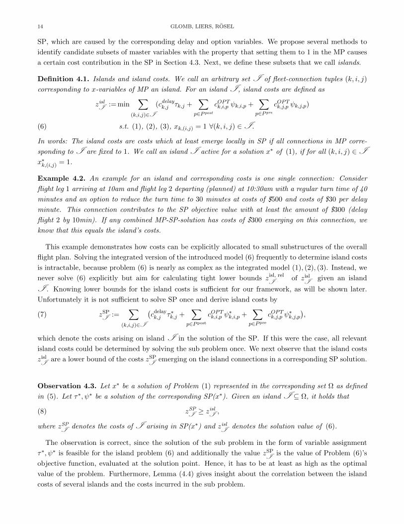
Definition 4.1. Islands and island costs. We call an arbitrary set I of fleet-connection tuples (k, i, j)

corresponding to x-variables of MP an island. For an island I , island costs are defined as

zislI

:= min∑

(k,i,j)∈I

(cdelayk,j τk,j +∑

p∈P post

cOPTk,i,p ψk,i,p +∑p∈P pre

cOPTk,j,p ψk,j,p)

s.t. (1), (2), (3), xk,(i,j) = 1 ∀(k, i, j) ∈ I .(6)

In words: The island costs are costs which at least emerge locally in SP if all connections in MP corre-

sponding to I are fixed to 1. We call an island I active for a solution x∗ of (1), if for all (k, i, j) ∈ Ix∗k,(i,j) = 1.

Example 4.2. An example for an island and corresponding costs is one single connection: Consider

flight leg 1 arriving at 10am and flight leg 2 departing (planned) at 10:30am with a regular turn time of 40

minutes and an option to reduce the turn time to 30 minutes at costs of $500 and costs of $30 per delay

minute. This connection contributes to the SP objective value with at least the amount of $300 (delay

flight 2 by 10min). If any combined MP-SP-solution has costs of $300 emerging on this connection, we

know that this equals the island’s costs.

This example demonstrates how costs can be explicitly allocated to small substructures of the overall

flight plan. Solving the integrated version of the introduced model (6) frequently to determine island costs

is intractable, because problem (6) is nearly as complex as the integrated model (1), (2), (3). Instead, we

never solve (6) explicitly but aim for calculating tight lower bounds zisl, rel

Iof zisl

Igiven an island

I . Knowing lower bounds for the island costs is sufficient for our framework, as will be shown later.

Unfortunately it is not sufficient to solve SP once and derive island costs by

(7) zSPI

:=∑

(k,i,j)∈I

(cdelayk,j τ∗k,j +

∑p∈Ppost

cOPTk,i,p ψ∗k,i,p +

∑p∈Ppre

cOPTk,j,p ψ∗k,j,p

),

which denote the costs arising on island I in the solution of the SP. If this were the case, all relevant

island costs could be determined by solving the sub problem once. We next observe that the island costs

zislI

are a lower bound of the costs zSPI

emerging on the island connections in a corresponding SP solution.

Observation 4.3. Let x∗ be a solution of Problem (1) represented in the corresponding set Ω as defined

in (5). Let τ∗, ψ∗ be a solution of the corresponding SP(x∗). Given an island I ⊆ Ω, it holds that

(8) zSPI≥ zisl

I,

where zSPI

denotes the costs of I arising in SP(x∗) and zislI

denotes the solution value of (6).

The observation is correct, since the solution of the sub problem in the form of variable assignment

τ∗, ψ∗ is feasible for the island problem (6) and additionally the value zSPI

is the value of Problem (6)’s

objective function, evaluated at the solution point. Hence, it has to be at least as high as the optimal

value of the problem. Furthermore, Lemma (4.4) gives insight about the correlation between the island

costs of several islands and the costs incurred in the sub problem.


Lemma 4.4. Let x∗ be a solution of Problem (1) and let E be a collection of pairwise disjoint Islands

which are active for x∗. Then it holds that zSP ≥∑

I ∈E zislI

.

Proof. We prove first that the cardinality |j ∈ L | ∃k ∈ K, i ∈ L,I ∈ E : (k, i, j) ∈ I | is either 0 or 1.

Assume it is not true, then there exist (k, i, j) 6= (k′, i′, j) with x∗k,(i,j) = x∗k′,(i′,j) = 1. In case k = k′ this

contradicts Constraint (1b), since the left side of the constraint evaluates to 2 and the right side is binary.

In case k 6= k′, Constraint (1b) implies that y∗k,j = y∗k′,j = 1. This contradicts Constraint (1d) since the

left side evaluates to 2 6= 1. Similar arguments apply to |i ∈ L|∃k ∈ K, j ∈ L,I ∈ E : (k, i, j) ∈ I |.Hence, rearranging the following sum is possible, since it is assured that no summand appears twice on

the left side, whereby τI , ψI are part of the solutions of (6) for every I :∑I ∈E

zislI

=∑I ∈E

∑(k,i,j)∈I

(cdelayk,j τIk,j +

∑p∈Ppost

cOPTk,i,p ψIk,i,p +

∑p∈Ppre

cOPTk,j,p ψIk,j,p)

Obs. 4.3≤

∑I ∈E

∑(k,i,j)∈I

(cdelayk,j τ∗k,j +

∑p∈Ppost

cOPTk,i,p ψ∗k,i,p +

∑p∈Ppre

cOPTk,j,p ψ∗k,j,p)

rearrange≤

∑k∈K

∑j∈Lk:∃i∈Lk,I ∈E :(k,i,j)∈I

cdelayk,j τ∗k,j

+∑k∈K

∑i∈Lk:∃j∈Lk,I ∈E :(k,i,j)∈I

∑p∈Ppost

cOPTk,i,p ψ∗k,i,p

+∑k∈K

∑j∈Lk:∃i∈Lk,I ∈E :(k,i,j)∈I

∑p∈Ppre¸

cOPTk,j,p ψ∗k,i,p

add positive terms≤

∑k∈K

∑l∈Lk

cdelayk,l τ∗k,l +

∑k∈K

∑l∈Lk

∑p∈P

cOPTk,l,p ψ

∗k,l,p = zSP

This is exactly the statement of the lemma.

Next we show how easy-to-solve relaxations of Problem (6) can be determined. Hence, an observation is

presented which describes the solutions of Problem (6), when the Aircraft Assignment model constraints

are dropped. It serves as the theoretical substantiation of the following steps.

Observation 4.5. Let P be Problem (6) for island I dropping system (1) and let F be the set of all

fleet-flight combinations which are not included in I , namely

F := (k, l) ∈⋃k′∈Kk′ × Lk′ \ (k′, l′) : ∃j : (k′, l′, j) ∈ I ∨ ∃i : (k′, i, l′) ∈ I .

Then an optimal solution for P exists, in which the variables yk,l, ςk,l, εk,l, τk,l and for all p ∈ P the

variables ςk,l,p, εk,l,p, δk,l,p, ψk,l,p, as well as w, θ corresponding to the fleet-flight combinations (k, l) ∈ F

have value 0.

Observation 4.5 states, that only x-variables contained in the island have to be considered. Therefore,

the ground process model (2) has to be included only partially as well, containing all time (ς, ε), duration

(δ), delay (τ) and option (ψ) variables associated with connection-fleet or flight-fleet combinations con-

tained in I . The turnaround resource model (3) is introduced for all hubs where a resource shortage can

occur. In this case, all resource flow (w) and resource transmission (θ) variables are taken into account

which are associated with connection-fleet and flight-fleet combinations belonging to the relevant Island


I . For some islands there is no risk for resource shortages and hence all constraints and variables of (3)

are left out. We discuss this in more detail later.

4.3. Island Identification. In this section we present approaches to find different types of islands. These

types differ by the computational effort of identifying them and finding lower bounds zisl, rel

Ifor their

corresponding island costs zislI

. In the following we will describe four different types of islands and explain

how they can be identified.

Single Connection Island (SC).

A large part of costs occuring in the SP in form of turnaround or delay costs are not caused by the flight

string or the scarcity of resources. They are caused by single flight connections which imply too short

periods of time between the arrival and departure of the connected flights. This in turn leads to the

fact that not all necessary turnaround processes can be carried out between the two subsequent flights.

In this case |I | = 1, which means that costs of optional turnaround quickening and delay costs of the

connected flight are just weighed against each other and the most favorable combination is selected. For

(SC)-islands, island costs are positive on connections (i, j), which do not include enough time on ground

to perform all turnaround steps if executed by fleet k. On connections of this kind, either costs for the

turnaround processes on ground of (i, j) or delay costs for the outbound flight j arise. Hence the problem

relaxation of Model (6) is the following for single-connection islands I = (k, i, j):

zisl, rel

I:= min cdelay

k,j τk,j +∑

p∈Ppost

cOPTk,i,p ψk,i,p +∑

p∈Ppre

cOPTk,j,p ψk,j,p

s.t. (2b)-(2j) with Lk= i, j, Ak= (i,j), K= k, xk,(i,j) = 1(9)

This model contains only 2|P |+ 3 binary variables of which three are fixed to 1. In addition, w.l.o.g. |P |many variables take the value 0. The Algorithm, which describes how to define an (SC)-island per given

connection and how to provide the corresponding island costs is part of the appendix.

The costs of all (SC)-islands can be calculated before optimizing the SP, or even the MP. This is possible

because the number of connections per fleet is bounded quadratically by the number of considered flight

legs, which can be executed by this fleet. Looking at real flight plans, one rarely comes close to this bound

and therefore this procedure does not influence the runtime perceptibly.

Single Flight String Island (SF).

Since costs are not only induced by single flight connections, flight sequences on individual flight strings

have to be investigated as well. The idea is that all costs occurring on parts of one flight string are intrin-

sically caused by this flight sequence. An (SF)-island depends on chosen flight sequences and therefore

depends on a feasible solution of the MP. It starts at a connection (i, j) executed by some aircraft of

type k ∈ K with positive costs or positive delay/delay costs on flight leg j. The end connection of a

(SF)-island is a connection (h, l) with 0 delay on flight leg l and island costs on (i, j), ..., (h, l) being

equal to the island costs on (i, j), ..., (h, l), (l,m) reduced by the (SC)-island costs on (l,m). These

conditions are checked along a flight string successively until the end connection is obtained and the island

is determined. The corresponding lower bound for the island costs are calculated by solving the following


String 1

String 2

String 3

HAM FRA BER FRA DRS

FRA HAM BER FRA BER

FRA HAM FRA DRS FRA

Flight

Turnaround Process

Aircraft Connection


Figure 7. (SF)-island consisting of consecutive flight connections detected on one singleflight string

relaxation of Model (6):

zisl, rel

I:= min

∑(k,i,j)∈I

(cdelayk,j τk,j +

∑p∈Ppost


p∈Ppre

cOPTk,j,p ψk,j,p)

s.t. (2), xk,(i,j) = 1 ∀(k, i, j) ∈ I , xk,(i,j) = 0 ∀(k, i, j) /∈ I .(10)

Problem (10) includes significantly fewer variables and constraints compared to Problem (6), since the

resource routing is neglected. Moreover, the problems can be optimized without having to calculate a

solution of the SP beforehand. This is necessary because costs for (SF)-islands must be calculated solving

Problem (10) whenever the solution of the MP implies new flight sequences. The Algorithm, which

describes how (SF)-islands are generated and the corresponding costs are calculated can be found in the

appendix. It can be divided into two components. First, the costs on a given flight string are weighed

against each other from a certain connection as described to identify the relevant flight string part. Then,

Problem (10) is solved to compute the cost associated with the island.

Multiple Flight Strings Island (MF).

In order to determine candidates for (MF)-islands, we compare the delay and cost structure along flight

strings in the SP with and without resource tracking constraints consisting of Model (3). The procedure

is the following: it is iterated along flight strings (determined by the MP) for each aircraft. For each

flight connection we compare costs caused by this connection (option and delay costs) and the delay

on the outgoing leg of this connection in the (SF)-island calculation model (the model without resource

constraints) and in the SP model (with resource constraints included).

We denote the corresponding delay and costs arising on one connection in the SP as the (SP)-delay

and (SP)-costs, the delay and costs arising in the (SF)-islands as (SF)-delay and (SF)-costs. Here, four

different cases can occur, which depend on the behaviour of the sub problem solution including resource

routing constraints and are precisely described in Table 4. In the cases 1 and 2 resource bottlenecks have

to be considered before the relevant connection and in case 3 and 4 these bottlenecks occur after the

relevant connection.

Based on these insights we propose a heuristic procedure to determine conflicting connections which

cause resource bottlenecks at hub-airports. If the bottleneck is expected before a certain connection (Case

1, Case 2), we go through the processes of the dedicated connection and look for predecessor processes

with a tight time dependency in the current SP solution. There is a tight time dependency between two

processes p1, p2 on flight legs l1, l2 served by fleet k1, k2 if they successively use the same resource r on

airport s and

ε∗k1,l1,(s,r) + dtrans(s,r) ≤ ς∗k2,l2,(s,r)


Case Setting Description1 (SP)-delay > (SF)-delay,

(SP)-costs ≥ (SF)-costsIf the connection is the first connection on the current flightstring section a deviation is caused on the airport of the con-nection because of resource shortages during some turnaroundprocess on the connection. Hence it is necessary to look for re-source bottlenecks immediately before the current connection.

2 (SP)-delay > (SF)-delay,(SP)-costs < (SF)-costs

In the SP-solution costs are omitted by permitting higher de-lays due to a later turnaround resource shortage on the flightstring. Hence one has to look for resource bottlenecks beforethe current connection and before subsequent connections ofthe flight string at hub-airports.

3 (SP)-delay ≤ (SF)-delay,(SP)-costs > (SF)-costs

More costs to save time emerge in the SP-solution. On theobserved connection or a later one of the flight string someprocess has to be finished earlier, so resource shortages occuron subsequent connections of the flight strings located at hub-airports after or during the connection’s turnaround processes.

4 (SP)-delay ≤ (SF)-delay,(SP)-costs ≤ (SF)-costs

This behavior is caused by a Case 3 on a predecessorconnection; it is proceeded with the predecessor connection.

Table 4. Case distinction for different settings which compare delay and costs on oneconnection in the SP and in Problem (10)

derived from constraints (3e) and (3f) holds with equality. This means that there is no time between the

end of the first process and the start of the transfer as well as between the end of the transfer and the start

of the second process. For flight legs l1, l2, we determine all flights passing the turnaround simultaneously

via i ∈ Ls,r : ε∗ki,i ≥ ε∗k1,l1 , ς∗ki,i≤ ς∗k2,l2, i.e., exactly the flight legs that are prioritized over l in terms of

resource allocation. All connections on hub-airports corresponding to the flights detected are considered

as conflicting.

In Case 3 and 4 we look for successor processes with an almost tight time dependency, i.e., if l1 is the

current processes flight and l2 is the successor processes flight, and k1, k2 are the currently assigned fleets,

ε∗k1,l1,(s,r) + dtrans(s,r) ≤ ς∗k2,l2,(s,r)

derived from constraints (3e) and (3f) holds with a slack of at most the amount of time difference of

the current acceleration option compared to the next cheaper acceleration option. The determination of

conflicting flight legs is equivalent to the procedure above.

Once all resource conflicts are detected, we unite (transitively) the (SF)-islands of connections which

are in conflict with each other to (MF)-islands. The island costs are estimated by solving a reduced

version of problem (6), incorporating only connections which are contained in the island:

zisl, rel

I:= min

∑(k,i,j)∈I

(cdelayk,j τk,j +

∑p∈Ppost


p∈Ppre

cOPTk,j,p ψk,j,p)

s.t. (2), (3), xk,(i,j) = 1 ∀(k, i, j) ∈ I , xk,(i,j) = 0 ∀(k, i, j) /∈ I .(11)

The overall procedure to identify (MF)-islands and the corresponding island costs can be seen in the

appendix. Given an initial (SF)-island, it searches for conflicts on each included connection. Therefore

the pool of connections which has to be checked for conflicts grows larger. When no connections are left

to be checked, the algorithm obtains a (MF)-island by combining all (SF)-islands which include at least

one conflicting connection. In the end, Problem (11) is solved to obtain the corresponding island costs.


String 1

String 2

String 3

HAM FRA BER FRA DRS

FRA HAM BER FRA BER

FRA HAM FRA DRS FRA

Flight

Turnaround Process

Aircraft Connection


Figure 8. (MF)-island detected over flight strings which are connected by turnaroundevents taking place at the same hub-airport in similiar time windows

The largest possible islands consists of every connection which is chosen. Although (MS)-islands pro-

duce the weakest cuts, the exact “calculation” of the corresponding island costs is very easy. They

guarantee the overall algorithm to be finite.

Master Solution Island (MS).

(MS)-islands consist of all connection variables selected in the current MP solution. Hence, one (MS)-

island is created in every decomposition iteration whenever the complete SP is optimized. The island

costs are equal to the objective value of SP. The constraints added to the MP for this kind of island

are equivalent to the no-good-cuts in the basic decomposition presented in Section 4.1. The usage of

(MS)-islands ensures that all SP costs will be covered and that the overall procedure terminates.

4.4. Combining Islands to generate Cuts.

Whenever a new island I is detected (no matter which type) and corresponding island costs zislI

are

calculated, the island is saved in the set E , the island pool. Furthermore, a variable σI is added to the

master problem, together with the additional constraint

(12) σI ≥ zisl, rel

I(∑

(i,j,k)∈I

xk,(i,j) + 1− |I |).

For a given MP solution x∗ we call an island I ∈ E active, if (k, i, j) ∈ I ⇒ x∗k,(i,j) = 1. The

variables σI are to interpret as “if an island I is active, then the variable σI takes the island costs

as value, otherwise 0”. They express a part of the sub problem costs caused by specific structures in

the MP solution. The σI -variables cannot be directly incorporated into the master problems objective

function, since two active islands I and I ′ do not necessarily have to be disjoint. Whenever this

happens, the sum σI + σI ′ may overestimate the local SP costs if both I and I ′ are active.

However, if E ′ ⊆ E is a subset of disjoint and active islands, it holds that the sum of the respective

island costs is at most the SP objective value:

(13) zSP ≥∑I ∈E ′

zisl, rel

I.

One can exploit this property by bounding the single variable σ incorporated in the objective of the

MP from below. Whenever a new MP solution is calculated, a set packing problem is solved, which


determines a family of disjoint islands E ∗ ⊆ E , maximizing the RHS of Equation (13):

maxE ′⊆E

∑I ∈E ′

zisl, rel

I

s.t.I ∩I ′ = ∅ ∀I ,I ′ ∈ E ′ : I 6= I ′

I active for x∗ ∀I ∈ E ′(14)

It is straight-forward to reformulate this problem into a binary linear program, which can be solved

with standard software. The optimal value of Problem (14) is compared to the current value σ∗ of the

master variable σ. In case the optimal value is greater than σ∗, the constraint

(15) σ ≥∑I ∈E ∗

σI

is added to the MP, cutting off the current solution. The MP is solved again. In case σ is equal to the

optimal value, additional islands will be generated.

Algorithm 1 Island Decomposition Algorithm

1: INPUT: Overall problem instance (1), (2), (3)2: OUTPUT: Solution for (1) and (2), (3)3: procedure Decomposition((1), (2), (3))4: Split problem into MP (1) and SP (2), (3)5: Initialize float zSP ←∞, σ∗ ← 06: Initialize (SC)-island pool E(SC) ← generate sc island((2), (k, i, j)) ∀xk,(i,j) in (1)7: Initialize island pool E = E(SC) and (SF)-island pool E(SF) = 8: Solve MP, solve SP based on MP solution → feasible solution of the integrated model9: do . outer loop

10: do . middle loop11: do . inner loop12: Ω,F , x∗, σ∗ ← Solve MP13: E ∗ ← Solve Model (14) depending on x∗

14: Add Cut (15) depending on E ∗ to MP

15: while σ∗ <∑

I ∈E ∗ zisl, rel

I16: E new

(SF) ← generate sf island((2), (k, i, j), Fk, E(SC)): (k, i, j) ∈ Ω \ E

17: Add E new(SF) to E(SF) and E

18: while E new(SF) 6= ∅

19: SP∗, zSP ← Solve SP20: E new

(MF) ← generate mf island((2), (3), Ω, SP∗, E(SF), B): B ∈ E(SF) with B ⊆ Ω\E21: E new

(MS) ← (Ω, zSP) \ E . add (MS)-island

22: Add E new(MF) and E new

(MS) to E

23: while σ∗ 6= zSP

24: return Ω, SP∗

25: end procedure

4.5. The overall Island Decomposition algorithm. In this section the overall Algorithm 1 is set up.

It starts with splitting the complete problem in MP and SP in line 4 as described above. Subsequently,

MP as well as SP are solved once, to determine a first feasible solution as reference in line 8. After

this step all (SC)-islands are calculated and initialize the island pool E . Then the inner loop (lines 11-

15) is executed: It resolves the MP, composes sets of active islands solving Model (14) and inserts the


corresponding cut to the MP as long as the MP solution varies. Afterwards new (SF)-islands are generated

in the middle loop (line 16). If at least one new (SF)-island is found, it is added to the island pool E

and it is repeated with the inner loop. Otherwise, the entire SP is solved once and the corresponding

(MS)-island and (MF)-islands are added to the island pool as well (lines 21,20). Then the entire outer

loop is repeated until the estimation of the SP costs σ∗ equals the actual SP costs zSP. If this is the case,

the problem is solved to optimality and the solution (for MP and SP) is returned as output.

Master Problem MP (Aircraft Assignment Model)

Variables: x (integral), y (integral), σ

OuterLoop

MiddleLoop

Sub Problem SP (Process Scheduling & Resource Allocation)

Variables: ψ (integral), w (integral), ς, ε, δ, τ , θ

Objective: zSP

Relaxed SP(Island Cost Calculation)

Individually defined

x∗ x∗(I , σI )

x∗, ς∗, τ∗,δ∗, ε∗, ψ∗,θ∗, w∗, zSP

Figure 9. Scheme of the procedure for Island Decomposition using relaxed versions ofthe SP to calculate islands and island costs

Theorem 4.6. Algorithm 1 terminates after a finite number of steps and returns an optimal solution for

the integrated tail assignment and ground process management problem (1)+(2)+(3).

Proof. The Aircraft Assignment problem (1) has a finite number of solutions. If the outer loop is run twice

and the same master and sub solution are generated in each iteration, then the algorithm terminates,

since in the first iteration the (MS)-island cut has been added to the MP. Due to Observation 4.3 it holds

that in every other inner or middle loop iteration when this solution has been the current master solution,

the SP cost bound has been at most the cost value of the (MS)-island. Hence, in the second outer loop

iteration with the solution, the condition σ∗ = zSP is fulfilled and the algorithm terminates.

An analogous argument holds for the middle loop, which generates (SF)-islands. This procedure is

uniquely determined by the current MP solution. Hence, when there are two iterations with the same

master solution, the (SF)-islands corresponding to the island are already contained in the island pool E .

Therefore the middle loop is executed a finite number of times. The same argument holds for the inner

loop regarding repetitive solutions of the MP. We have shown that the algorithm terminates after a finite

number of steps with a feasible solution of the integrated problem.

In order to show its optimality, we consider x∗ the solution of the master problem which is returned by

the algorithm. We assume a solution x′ of the master problem exists with zMP(x′) + zSP(x′) < zMP(x∗) +

zSP(x∗). Since the MP in line 12 has been solved to optimality, we can derive the existence of a constraint

in the MP which enforces σ ≥ zSP(x′). Since Observation 4.3 together with Observation 4.5 assure that

the generate x islands routines deliver lower bounds for the true island costs, and Lemma 4.4 assures

that whenever this is the case, the inner loop only adds constraints to the MP which have the property

that σ underestimates the value of zSP, this is a contradiction.

Hence, the solution delivered by Algorithm 1 is optimal, which is exactly the required result.

In the following section we prepare our computational study by introducing how we derive different

instance sets using real-world flight schedules. In addition, we propose two benchmark algorithms which

are used to evaluate the Island Decomposition approach.


5. Baseline Algorithms and Instance Sets

Since the model presented is a novel model, this chapter will focus on two important aspects: First, it

will be shown how the instances for the subsequent computational study are generated. Afterwards we

present two benchmark algorithms, which can also be used to solve the problem.

5.1. Generating Instance Sets. All of our instances are based on a real flight plan of a major German

airline. However, this plan includes the flights of a whole week of all countries that are served. Our problem

is more suitable for monitoring individual days in certain areas, since crucial turnaround decisions do not

have to be planned for all days and only take place at hub-airports. In order to generate adequate

instances, we rely on the common large base schedule, also containing information regarding the available

fleets, from which individual sub-instances are derived. To avoid unrealistic instances, we first reduce the

plan to a certain selected set of flights and airports, which must contain at least one hub.

We have reduced the turnaround sequence to four representative steps: De-Boarding, Catering, Clean-

ing and Boarding, containing two turnaround steps which require the same resource as well as sequential

and parallel turnaround processes. Hence, the reduction of turnaround processes does not influence the

structure or optimization behavior of the solution algorithms, but limits the computational effort.

We created instances in a random interval of flights and aircraft. Feasible solutions should utilize the

whole aircraft fleet while covering all flights of the given schedule. The ratio between flights and aircraft as

well as the structure of each schedule should lead to adequate, but relatively tight time windows between

arrivals and departures of subsequently executed flight legs.

To generate this kind of instances, a reduced tail assignment problem is solved beforehand. The problem

is defined on the base schedule. Its surrogate objective function minimizes the number of used aircraft,

including a randomly given number of flight legs. The assignment costs for each fleet-flight pair were

selected arbitrarily as well to be able to vary the instances. The solution yields all flights and aircraft

which will be used in our instance from now on. Based on the selected connections of this reduced problem

solution and the resulting ground times, turnaround processes were timed by splitting the overall ground

time per connection. To provoke delays which result in interesting instances, the critical path of the

turnaround process chain is designed not to fit entirely into the corresponding ground time interval on

some connections. Additionally, a random number of resources per process is selected at the hub-airport.

This number is chosen to provoke resource shortages at some points for the same reason. Thus it has to

be drastically lower than the number of aircraft used in order to exclude situations where the resource

limitation is not restrictive. All parameters and quantities listed in the model are added based on random

intervals. All assignment decisions of this preliminary optimization procedure are discarded afterwards.

Instance Set I1 I2# Instances 50 50# Flights 38-102 38-104# Airports 3-8 3-8# Aircraft 5-12 5-13Ground interval 30-80min 30-80minProcess duration factor 1.01 - 1.24 1.1-1.35Resource factor 0.25 0.5

Table 5. Characteristics of I1 (small resource factors) and I2 (long process duration)

For our computational results we generated two instance sets I1 and I2. Instance set I1 has tightly

timed process steps, which partly exceed the possible ground times and has very few resources on ground


available as is usual in practice. Instance set I2 has tighter timed process steps but is less restrictive re-

garding ground resources. We expect the necessity of adding more (MF)-islands during the decomposition

procedure to get high quality results for I1. Both Instance sets contain 50 instances. All characteristics

per instance set are summarized in Table 5. The random numbers are the result of randomizing the sizes

of instances while preserving realistic flight schedules, i.e., without too much time between two consecu-

tive flights and just enough aircraft to execute all flights. In the calculated reference solution of the Tail

Assignment problem only connections with ground times between 30 and 80 minutes can be selected.

The main differences between I1 and I2 are different values for the process duration factor and the

resource factor. For each of the instances, the time necessary to carry out turnaround processes is

constructed such that the turnaround duration slightly exceeds the ground time between two flights in a

reference solution. Hence, the duration of the the entire turnaround process is calculated by the product

of the process duration factor and with the time spent in the reference solution on the ground. This value

was chosen to replicate external factors on the basis of which delays occur. The process duration factor

for I1 is set to smaller values because we do not want to distort the resource bottleneck observations.

Each single instance has more than one process duration factor, one for each aircraft type.

The number of resources available on each hub-airport is calculated with the formula max(1, b0.5 +∑k∈K |Qk| · ρc + α), whereby Qk is the set of aircraft of fleet k as defined in Table 1, ρ is the resource

factor defined in Table 5 and α is randomly drawn from −1, 0, 1. The formula’s goal is to put the

number of resources available in an appropriate ratio to the aircraft available and to vary it slightly.

5.2. Benchmark algorithms. In order to evaluate the solution quality of the Island decomposition

algorithm, we present two further solution approaches that could typically be used for this type of problem.

We first tried to compare the solution characteristics of the decomposition approach with solving the

integrated model (1) + (2) + (3). Unfortunately, it turned out that the integrated solving of the problem

spent a large amount of time on finding only a feasible solution to the problem in the first place.

Thus we concluded that it is beneficial to generate a feasible start solution by first solving model

(1), fixing all the variables and solve (2) + (3) afterwards. As discussed in the previous sections, this

always leads to a feasible solution of the whole problem. This solution is used as a start solution for the

MIP-Solver. The procedure of improving this start solution is called Benchmark Waterfall.

We also want to compare our approach against alternative decomposition approaches. Our approach

has many aspects in parallel to Benders decomposition: The problem is split into master and sub problem.

The master problem is solved and based on the solution the right-hand side of the subproblem changes.

Afterwards the solution of the subproblem makes it possible to derive valid inequalities bounding the

objective of the master problem. However, the standard version of Benders decomposition is not capable

of taking integral variables in the sub problem into account. There exist integral versions of Benders

decomposition, but they do not seem to perform well in practice. Many authors apply the standard version

using the continuous relaxation of the sub problem and calculate an integral solution of the sub problem

after the master variables are fixed. The behaviour of the solution calculated by the approach can be

simulated by solving the integrated model while relaxing the integrality constraints of the sub problem,

fixing the master variables, reintroduce integrality constraints and calculate the sub problem solution.

Analogously to Benchmark Waterfall one can use the obtained solution of Benders decomposition as a

start solution for solving the integrated model. We call this approach Benchmark Benders.


6. Computational Results

The Island Decomposition approach is compared with the benchmark algorithms that are evaluated for

two described instance sets. Our model is intended to adjust parts of existing plans on the day before

operations, so that currently known ground conditions can be optimally planned. We first investigate

with a mean value study of I1 whether the Island Decomposition can find high-quality solutions in an

acceptable time. Furthermore, we check whether better solutions can be found faster than using the

benchmark algorithms. We believe that for I1 with resource bottlenecks the (MF)-islands will be crucial.

In the further setting with instance set I2 we will investigate if the decomposition approach still gives

good results if there are more than enough resources on the ground.

All algorithms are implemented in Python 3.7.1 and all MIPs are solved with Gurobi 9.1.1, see

Gurobi Optimization (2020). The computations were executed on a 4-core machine with a Xeon E3-

1240 v6 CPU (3.7GHz base frequency) and 32 GB RAM.

In the following we present the results of the computational study, containing comparison of runtimes,

solution quality, performance profiles and dependencies of the solution behavior on instance characteristics.

6.1. Results of the Computational Evaluation.

In the following, we will analyze the results of the computations which deal with solving the instances

from I1 using Island Decomposition and the benchmark algorithms listed in Section 5.

2.00%

4.00%

6.00%

8.00%

10.00%

12.00%

14.00%

0

30

0

60

0

90

0

12

00

15

00

18

00

21

00

24

00

27

00

30

00

33

00

36

00

Gap

in %

Time in s

Island Decomposition Benchmark Benders Benchmark Waterfall

Figure 10. I1: Mean optimality gap over time for Island Decomposition and benchmarks

Figure 10 shows the mean value of the gaps of all instances in I1 over the solution time. The mean gap

for the decomposition approach is lower than the mean gap for the benchmark approaches at all points

in time. The curve for the Island Decomposition drops heavily at the beginning of the calculations, since

all (SC)-islands estimate the costs right from the start. In the further course, the mean gap decreases

less heavily. It should be noted that any steps in the curve indicate that some instances could be solved

completely optimally. The decomposition approach yields a mean gap of just over 3% after one hour,

whereas the benchmark approaches have a gap of about 8%. One can observe that the Benchmark

Benders approach, although it starts with a better initial solution and therefore has a smaller initial gap,

is outperformed by the Benchmark Waterfall approach, which has a worse initial solution. Nevertheless,

it seems to be much more effective at computing good valid lower bounds on the solution value and yields

lower optimality gaps for computation times above 300 − 450 seconds. We assume that the behavior is

due to the fact that the solution found by the Benchmark Benders has a better objective function value,

but is a solution from which the MIP solver cannot branch effectively. The proportions of different island


81.78%

12.06%

3.07% 3.09%

(SC) islands (SF) islands (MF) islands (MS) islands

48.65%

75.41%

87.03%

0.00%

20.00%

40.00%

60.00%

80.00%

100.00%

Ergebnis

Me

asu

rem

en

t o

f th

e a

ctu

al c

ost

s in

curr

ed

in %

(SC) Islands (SF) islands (MF) Islands

Figure 11. I1: Mean value of proportions of different island types after 3600 s (left side),I1: Percentage of costs in the SP that could be covered by each island type (right side)

types which were generated during the solution process is shown on the left side of Figure 11. Most of

the generated islands are (SC)-islands (81.78%). These are created at the beginning of each calculation,

regardless of whether the connection to which the island corresponds has ever been assigned or not. The

number of (SC)-islands predominates here, since islands are generated for all single connections at the

beginning of the calculation regardless of the MP solutions found. All other island types, which are

generated dynamically, just depend on relevant flight strings, which are selected in the MP solution.

Therefore and because not all possible flight strings are useful regarding the objective function of the MP,

the number of dynamically generated island types is significantly lower within one hour of computation.

It is clear that the rate of (SC)-islands gets smaller over time, since all of them are generated at the

beginning, while the number of all other island types grows with time. The (SF)-islands seem to be the

dominant type of islands calculated dynamically by the algorithm with a rather high proportion (12.06%).

The proportion of (MF)-islands (3.07%) is similiar to the one of (MS)-islands (3.09%). Note that even

though the percentage of dynamically generated islands may seem small, the effect of these islands is

crucial to the decomposition approach: The right side of Figure 11 shows what percentage of the actual

costs generated in the SP could be covered on average by the respective island type in the mean. We can

see that the (SC)-islands cover less than 50% of the costs, while the (SF)-islands already cover more than

75%. In addition, it is noticeable that during the solution process, additional 12% of the costs, which

obviously only arise from resource bottlenecks, can be covered by (MF)-islands in the MP.

Figure 12 shows the mean ratio of the current objective values to the best lower bounds found over all

time periods and algorithms within 60 minutes, calculated with the help of the following formula:

(16)inc(alg, t)− lb∗

lb∗,

where inc(alg, t) denotes the best incumbent value found by algorithm alg after t seconds of calculation

and lb∗ denotes the best lower bound over all algorithms and over the entire runtime. Figure 13 shows

the corresponding information in the form of the lower bound is described by the following formula:

(17)|lb(alg, t)− inc∗|

inc∗,

where lb(alg, t) denotes the best lower bound found by algorithm alg after t seconds of calculation and

inc∗ denotes the best incumbent value over all algorithms and over the entire runtime.

Figure 12 shows the actual solution quality of the algorithms: First, it can be seen that the Island

decomposition produces the best solutions again on average from about three minutes onwards. The


Benchmark Benders, on the other hand, starts with the best incumbent, but can hardly improve it over

the runtime. The Benchmark Waterfall is dominated by the other two algorithms over the entire runtime.

Looking at the lower bounds in Figure 13, we see that the decomposition approach finds tight lower

bounds very quickly, supporting the fact that the (SC)-islands are crucial for this. The Benchmark

Waterfall can continuously improve the lower bounds. In Benchmark Benders, it is noticeable that the

lower bound from the start can hardly be tightened.

2.00%

3.00%

4.00%

5.00%

6.00%

7.00%

8.00%

9.00%

10.00%

0

30

0

60

0

90

0

12

00

15

00

18

00

21

00

24

00

27

00

30

00

33

00

36

00

Incu

mb

en

t-R

atio

in %

Time in s


Figure 12. I1: Ratio Incumbent/Best LB - 1

2.00%

3.00%

4.00%

5.00%

6.00%

7.00%

8.00%

0

30

0

60

0

90

0

12

00

15

00

18

00

21

00

24

00

27

00

30

00

33

00

36

00

LB-R

atio

in %

Time in s


Figure 13. I1: 1 - Ratio LB/Best incumbent

We derive from Figure 12 that based on incumbents the Island Decomposition outperforms the bench-

mark algorithms comparing the solutions of I1. The same behaviour can be observed in Figure 13, which

shows that the lower bounds identified by the Island Decomposition algorithm are also much stronger.

Exploiting the problem structure, the decomposition approach can quickly approximate many costs of

the SP in the MP, providing good lower bounds on the total cost. Moreover, based on the information

MP solutions can be selected that reduce the total cost. In contrast the benchmark approaches directly

use commercial MIP solvers which continuously apply heuristics to determine good primal solutions. We

would like to note that surprisingly, the Benchmark Benders approach does not generate better solutions

than the Benchmark Waterfall , although it differs only by starting with a better initial MIP solution.

This seems to influence the solver’s branching, node selection, presolve or heuristics strategies, such that

it is less likely that better primal solutions and dual bounds can be obtained.

Up to this point only mean value data has been considered. Therefore we analyze the individual

results per instance. The decomposition approach finds most solutions between 0.0% and 0.5%. With the

exception of one outlier, all solutions have a gap of less than 11.5%. The Benchmark Waterfall can solve

some instances very well, but has a clustering point at around 13%. The Benchmark Benders rarely finds

a very good solution and most solutions are places in between 2.5% and 17.5%.

Island Decomposition and benchmark algorithms are exact solution approaches which deliver the opti-

mal solution in theory. Hence, we show how many of the instances could actually be solved to optimality.

Figure 14 plots the number of instances solved to optimality over time for each solution approach.

It can be seen that the Island Decomposition approach was able to solve 24 of 50 instances during

the whole time interval. Neither Benchmark Waterfall nor Benchmark Benders were able to solve any

instance to optimality. This clearly shows the strong benefit of our approach that is by far superior

to the benchmark methods tested here. In this category the Island Decomposition algorithm is clearly

dominating the benchmark algorithms. We believe this correlates with the fact that the MIP-solver cannot

find satisfactory lower bounds on either of the two benchmark approaches.

To give a better intuition on the gap distribution and to compare the algorithms more directly, we

present a performance plot in Figure 15. It is based on the best incumbent value the algorithms found


after 60 min of computation, which are compared to each other. It plots the proportion of instances which

could be solved by the respective algorithm to a smaller or equal incumbent value than the incumbent

value of the best algorithm for the corresponding instance multiplied with the value on the x-axis.

Figure 15 shows that the Island Decomposition approach provides the best incumbent value for 76% of

all instances and finds a good incumbent solution which is within approximately 1-1.05% of the incumbent

value the best of the three algorithms found for almost all instances. Contrarily, Benchmark Benders

delivers the best solution for 16% of all I1-instances and Benchmark Waterfall for 6% of the instances.

0

5

10

15

20

25

30

35

40

45

50

0

30

0

60

0

90

0

12

00

15

00

18

00

21

00

24

00

27

00

30

00

33

00

36

00

Nu

mb

er

of

solv

ed

Inst

ance

s (G

ap 0

.0%

)

Time in s


Figure 14. I1: Solved Instances

0.0

0.1

0.2

0.3

0.4

0.5

0.6

0.7

0.8

0.9

1.0

1.0

00

1.0

10

1.0

20

1.0

30

1.0

40

1.0

50

1.0

60

1.0

70

1.0

80

1.0

90

1.1

00

1.1

10

1.1

20


Figure 15. I1: Performance Plot

The results from I1 prove that Island Decomposition can quickly provide very good results and further-

more solve many instances, in contrast to the less efficient benchmark approaches. Moreover, in the case

of resource bottlenecks, the (MF)-islands contribute significantly to the cost representation in the MP.

Instance set I2 represents the setting with more resources on ground. We expect less costs to be incurred

by missing resources and more costs occuring directly due to flight connection combinations.

2.00%

4.00%

6.00%

8.00%

10.00%

12.00%

14.00%

0

30

0

60

0

90

0

12

00

15

00

18

00

21

00

24

00

27

00

30

00

33

00

36

00

Gap

in %

Time in s


Figure 16. I2: Mean optimality gap over time for Island Decomposition and benchmarks

Taking into account more resources on ground, I2 makes it easier to solve (3). Therefore we anticipate

that the benchmark algorithms will be able to find feasible and near-optimal solutions much faster than

in the computations of I2. The left side of Figure 16 shows that the mean gap for Island Decomposition

is also lower than the mean gap for the benchmark approaches at all points in time. After one hour of

computation, the Island Decomposition gap remains on average slightly lower than both Benchmark gaps.

The comparison of the two benchmark approaches shows the same behavior as for I1. The Benchmark

Benders finds a very good solution at the beginning, but from 5 minutes onwards, Benchmark Waterfall

delivers better results, which remains the same up until the end. The proportions of different island types

are depicted on the left side of Figure 17. Most of the generated islands are still of type (SC) (88.64%). The


88.64%

10.59%0.25% 0.53%

(SC) islands (SF) islands (MF) islands (MS) islands

46.18%

85.08%88.67%

0.00%

20.00%

40.00%

60.00%

80.00%

100.00%

Ergebnis

Me

asu

rem

en

t o

f th

e a

ctu

al c

ost

s in

curr

ed

in %

(SC) islands (SF) Islands (MF) islands

Figure 17. I2: Mean value of proportions of different island types after 3600 s (left side),I2: Percentage of costs in the SP that could be covered by each island type (right side)

proportion of (SF)-islands has decreased slightly compared with the evaluation of I1 (10.59%). Significant

is the difference regarding the more complex island types: The percentage of (MF)-islands and (MS)-

islands is almost negligible. However, the right side of Figure 17 shows that also the effectiveness of

the (MF) and (MS)-islands decreases heavily: The percentage of costs in the SP that can be covered

by (SF)-islands increases by to 85.64% compared to I1. However, the share of additional costs that are

covered by (MF)-islands is only 3.5% more. This indicates that (MF)-islands are less useful here.

Figure 18 shows the mean ratio of the current objective values to the best lower bounds found over all

time periods and algorithms within 60 minutes, calculated with the help of Formula (16). The right side

of Figure 19 shows the corresponding lower bounds, calculated with the help of Formula (17).

Figure 18 shows clearly that the actual average incumbent of the Island Decomposition is worse than

for the benchmark approaches. The gap curve of the Island Decomposition is nevertheless better. This

can be explained Figure 19, which shows that the lower bounds found for the decomposition approach are

much tighter than those of the benchmark approaches. This is sufficient to keep the gap lower on average

than for the benchmark approaches. Probably the solution of the MP varies heavily by the added (SC)-

and (SF)-islands, since no special flight strings dominate. This variation can only be described by the

(MS)-islands, which leads to a slow convergence of the decomposition approach. The tight lower bounds

are also reflected in the number of instances which can be solved to optimality: Island Decomposition

can find optimal solutions for 15 instances, whereas both benchmark instances together can only solve 8

instances to a gap of 0.0%. All further evaluations did not lead to any particular results. On instance set

I2, the Island Decomposition approach on the whole is inferior, but still calculates good lower bounds.

1.00%

2.00%

3.00%

4.00%

5.00%

6.00%

7.00%

8.00%

0

30

0

60

0

90

0

12

00

15

00

18

00

21

00

24

00

27

00

30

00

33

00

36

00

Incu

mb

en

t-R

atio

in %

Time in s


Figure 18. I2: Ratio Incumbent/Best LB - 1

1.00%

2.00%

3.00%

4.00%

5.00%

6.00%

7.00%

8.00%

9.00%

0

30

0

60

0

90

0

12

00

15

00

18

00

21

00

24

00

27

00

30

00

33

00

36

00

LB-R

atio

in %

Time in s


Figure 19. I2: 1 - Ratio LB/Best incumbent


Summary. In the test run with instance set I1 one can observe that the Island Decomposition method

is superior to the benchmark algorithms. The approach could generate the solutions with the best solution

quality by far. In contrast to I2, this is not only due to better lower bounds, but also to better incumbent

values. The structure of the instance set makes it impossible for MIP-solver based benchmark approaches

to find optimal solutions within the time limit of 60 minutes, whereas Island Decomposition can solve

almost 50% of the instances up to optimality. In addition, the ratio of the islands changes. Thus, more

(SF)-islands, (MF)-islands and (MS)-islands are generated than during the computations of I1. Also for

instance set I2 the Island Decomposition approach could generate the solutions with the best solution

quality. However, this is not due to good primary solution values but tight lower bounds, which can be

found quickly. These also contribute to the fact that more instances are completely solved than with

the help of the benchmark approaches. In addition, mainly (SC) and (SF)-islands are generated. On

the basis of both instance sets it was possible to demonstrate that the Island Decomposition approach is

capable of providing tight lower bounds quickly. Our Island Decomposition perform by far best considering

instance set I1. This is really important, since especially this instance set is relevant in practice, because

many delay events on ground can be explained by such bottlenecks. From the results, we can also deduce

that whenever the resources on ground are not limited, the benchmark algorithms typically are more

efficient than Island Decomposition in computing primal solutions. Whenever the ground time between

connections almost fits to perform all necessary turnaround steps but resource bottlenecks exist, the Island

Decomposition is the better approach to obtain good feasible solutions.

7. Conclusion and Outlook

This paper has provided a new mathematical model to handle two operational tasks of airlines simul-

taneously: Aircraft Assignment and Turnaround Handling. Moreover we demonstrated that this model is

not straight-forwardly solvable with standard approaches for reasonable problem sizes. Hence we devel-

oped a combinatorial decomposition approach, mathematically proved its capability of solving the model

to optimality and presented and extensive computational study, which proves its effectiveness in pratice.

Our future research will aim at integrating additional problem aspects to make the presented model

more realistic and therefore attractive for practitioners.

Another research direction is to make the decomposition approach more efficient, for example by

incorporating some of the smaller island types directly into the master model. We presume that this

could lead to a large speed up while pertaining the property of the algorithm to be an exact one.

We believe that the introduced decomposition framework is not only applicable to the presented in-

tegrated tail assignment and ground process management model but can also be transferred to other

mathematical problems. The condition is that these problems can be splitted into master and sub prob-

lem such that the prior is combinatorial and the latter highly depends on its integer nature.

Acknowledgements

This research has been conducted in the framework of the research project OPs-TIMAL, financed by

the German Federal Ministry of Economic Affairs and Energy (BMWi).

References

Abara, J. (1989). Applying integer linear programming to the fleet assignment problem. Interfaces, 19(4):20–28.


Barnhart, C., Boland, N. L., Clarke, L. W., Johnson, E. L., Nemhauser, G. L., and Shenoi, R. G. (1998). Flight

string models for aircraft fleeting and routing. Transportation science, 32(3):208–220.

Cadarso, L. and de Celis, R. (2017). Integrated airline planning: Robust update of scheduling and fleet balancing

under demand uncertainty. Transportation Research Part C: Emerging Technologies, 81:227–245.

Clarke, L. W., Hane, C. A., Johnson, E. L., and Nemhauser, G. L. (1996). Maintenance and crew considerations in

fleet assignment. Transportation science, 30(3):249–260.

Codato, G. and Fischetti, M. (2004). Combinatorial benders’ cuts. In International Conference on Integer Pro-

gramming and Combinatorial Optimization, pages 178–195. Springer.

Codato, G. and Fischetti, M. (2006). Combinatorial benders’ cuts for mixed-integer linear programming. Operations

Research, 54(4):756–766.

Cordeau, J.-F., Stojkovic, G., Soumis, F., and Desrosiers, J. (2001). Benders decomposition for simultaneous aircraft

routing and crew scheduling. Transportation science, 35(4):375–388.

Dunbar, M., Froyland, G., and Wu, C.-L. (2012). Robust airline schedule planning: Minimizing propagated delay

in an integrated routing and crewing framework. Transportation Science, 46(2):204–216.

Eltoukhy, A. E., Wang, Z., Chan, F. T., Chung, S., Ma, H.-L., and Wang, X. (2019). Robust aircraft maintenance

routing problem using a turn-around time reduction approach. IEEE Transactions on Systems, Man, and

Cybernetics: Systems, 50(12):4919–4932.

Evler, J., Asadi, E., Preis, H., and Fricke, H. (2018). Stochastic control of turnarounds at hub-airports. Proceedings

of the Eighth SESAR Innovation Days, Salzburg, Austria, pages 3–7.

Glomb, L., Liers, F., and Roesel, F. (2020). A rolling-horizon approach for multi-period optimization.

Gopalan, R. and Talluri, K. T. (1998). The aircraft maintenance routing problem. Operations Research, 46(2):260–

271.

Gurobi Optimization, L. (2020). Gurobi optimizer reference manual.

Hane, C. A., Barnhart, C., Johnson, E. L., Marsten, R. E., Nemhauser, G. L., and Sigismondi, G. (1995). The fleet

assignment problem: Solving a large-scale integer program. Mathematical Programming, 70(1-3):211–232.

Papadakos, N. (2009). Integrated airline scheduling. Computers & Operations Research, 36(1):176–195.

Parmentier, A. and Meunier, F. (2020). Aircraft routing and crew pairing: updated algorithms at air france. Omega,

93:102073.

Sandhu, R. and Klabjan, D. (2007). Integrated airline fleeting and crew-pairing decisions. Operations Research,

55(3):439–456.

Sarac, A., Batta, R., and Rump, C. M. (2006). A branch-and-price approach for operational aircraft maintenance

routing. European Journal of Operational Research, 175(3):1850–1869.

Sherali, H. D., Bae, K.-H., and Haouari, M. (2010). Integrated airline schedule design and fleet assignment:

Polyhedral analysis and benders’ decomposition approach. INFORMS Journal on Computing, 22(4):500–513.

Sherali, H. D., Bae, K.-H., and Haouari, M. (2013). A benders decomposition approach for an integrated airline

schedule design and fleet assignment problem with flight retiming, schedule balance, and demand recapture.

Annals of Operations Research, 210(1):213–244.

Toth, P. and Vigo, D. (2014). Vehicle routing: problems, methods, and applications. SIAM.

Wu, C.-L. and Caves, R. E. (2004). Modelling and optimization of aircraft turnaround time at an airport. Trans-

portation Planning and Technology, 27(1):47–66.

Yan, C., Barnhart, C., and Vaze, V. (2020). Choice-based airline schedule design and fleet assignment: A decom-

position approach. Available at SSRN 3513164.

a novel decomposition approach for holistic airline

Documents