a novel decentralized economic operation in islanded ac ... · energies article a novel...
TRANSCRIPT
Aalborg Universitet
A novel decentralized economic operation in islanded AC microgrids
Han, Hua; Li, Lang; Wang, Lina; Su, Mei; Zhao, Yue; Guerrero, Josep M.
Published in:Energies
DOI (link to publication from Publisher):10.3390/en10060804
Creative Commons LicenseCC BY 4.0
Publication date:2017
Document VersionPublisher's PDF, also known as Version of record
Link to publication from Aalborg University
Citation for published version (APA):Han, H., Li, L., Wang, L., Su, M., Zhao, Y., & Guerrero, J. M. (2017). A novel decentralized economic operationin islanded AC microgrids. Energies, 10(6), [804]. https://doi.org/10.3390/en10060804
General rightsCopyright and moral rights for the publications made accessible in the public portal are retained by the authors and/or other copyright ownersand it is a condition of accessing publications that users recognise and abide by the legal requirements associated with these rights.
? Users may download and print one copy of any publication from the public portal for the purpose of private study or research. ? You may not further distribute the material or use it for any profit-making activity or commercial gain ? You may freely distribute the URL identifying the publication in the public portal ?
Take down policyIf you believe that this document breaches copyright please contact us at [email protected] providing details, and we will remove access tothe work immediately and investigate your claim.
Downloaded from vbn.aau.dk on: July 26, 2020

energies
Article
A Novel Decentralized Economic Operation inIslanded AC Microgrids
Hua Han 1, Lang Li 1, Lina Wang 2,*, Mei Su 1, Yue Zhao 3 and Josep M. Guerrero 4
1 School of Information Science and Engineering, Central South University, Changsha 410083, China;[email protected] (H.H.); [email protected] (L.L.); [email protected] (M.S.)
2 School of Automation Science and Electrical Engineering, Beihang University, Beijing 100191, China3 Department of Electrical Engineering, University of Arkansas, Fayetteville, AR 72701, USA;
[email protected] Department of Energy Technology, Aalborg University, DK-9220 Aalborg East, Denmark; [email protected]* Correspondence: [email protected]; Tel.: +86-135-2277-3516
Academic Editor: II-Yop ChungReceived: 16 April 2017; Accepted: 9 June 2017; Published: 13 June 2017
Abstract: Droop schemes are usually applied to the control of distributed generators (DGs) inmicrogrids (MGs) to realize proportional power sharing. The objective might, however, not suit MGswell for economic reasons. Addressing that issue, this paper proposes an alternative droop schemefor reducing the total active generation costs (TAGC). Optimal economic operation, DGs’ capacitylimitations and system stability are fully considered basing on DGs’ generation costs. The proposedscheme utilizes the frequency as a carrier to realize the decentralized economic operation of MGswithout communication links. Moreover, a fitting method is applied to balance DGs’ synchronousoperation and economy. The effectiveness and performance of the proposed scheme are verifiedthrough simulations and experiments.
Keywords: droop control; economic operation; microgrids (MGs); nonlinear droop
1. Introduction
Recently, interest has been concentrated on microgrids (MGs) [1–4], which represent an effectiveapproach to deal with distributed generation [5–8]. Usually, a MG comprises different types ofdistributed generators (DGs), such as diesel generators, wind turbines, photovoltaic (PV) generators,energy storage units, etc. Different DGs have different generation costs [9–11]. From the economicalperspective, less costly DGs should be controlled to provide more power and all DGs in the MGsshould be coordinated in economic operation modes [12–14].
The economical control approaches in MGs can be classified into the centralized, distributedand decentralized schemes. The centralized control in a hierarchical coordination control manneris proposed in [15], which can realize the optimal economic operation at steady state and ensurethe resilient response of MGs to emergencies. Further, reference [16] proposed another hierarchicalcoordination strategy for the economic operation of a community MG. Reference [17] proposed aheuristic method to solve the optimization problem, in which the total operation cost minimizationoperation can be obtained. The centralized control scheme possesses the advantages of economicoperation, better voltage and frequency regulation in MGs [18,19]. However, it requires globalinformation, complicated centralized controller and extensive communication networks, whichincreases the capital cost and system complexity, and reduces the reliability of MGs.
The distributed control schemes perform with neighbouring information, and need no centralizedcontrollers [20–23]. A distributed gradient algorithm is introduced in [23] to realize optimal generationcontrol. Further, the consensus algorithms are developed to solve the economic dispatch problem
Energies 2017, 10, 804; doi:10.3390/en10060804 www.mdpi.com/journal/energies

Energies 2017, 10, 804 2 of 18
in [24,25]. The incremental cost of each DG unit is selected as the consensus variable in [24] tominimize the total operation cost in a distributed manner. Another consensus algorithm is proposedin [25] to realize the equal incremental costs of each DG with a strongly connected communicationtopology. However, the control schemes in [23–25] are highly dependent on the communications forinformation exchange.
Recently, some scholars have solved the MG power dispatch problem using decentralizedapproaches [26,27], which require neither communications nor a centralized controller. The droopcontrol scheme is a classic decentralized control method. It has historically been applied to controlparalleled synchronous generators in a conventional power system [28,29]. In MGs, the droop controlschemes are used to control multiple DGs for proportional power sharing [30–33]. However, theeconomic operation of MGs is usually not guaranteed under the traditional droop scheme.
In order to reduce the generation cost of MGs, a linear cost prioritized droop scheme is presentedin [11] to reduce the total generation cost by setting a higher priority of the output power for thelower-cost DG. However, it might not be optimized efficiently due to the nonlinearity in the relationbetween the produced power and the generation cost. Further, in [34], a nonlinear droop schemewith cost performance index is introduced. The basic idea behind the method is to let the costly DGsoutput less power by designing the droop coefficients. The power sharing is based on equal generationcost rather than the optimal conditions of MGs, thus the economic operation is a suboptimal solutionin [34], but it is able to realize plug-and-play and has a wide range of practical value.
A nonlinear droop control strategy based on polynomial fitting method is utilized in [35], wherethe DG power outputs determined are based on the total generation cost of the MG. The synchronousoperation considering DGs’ capacity limitations is satisfied, however, the droop curve must beredesigned when any DG is added or removed, thus it is incapable of plug-and-play.
To address the above concerns, this paper proposes a droop control scheme for the decentralizedeconomic operation of MGs. It applies the optimization conditions to the typical droop control for thelowest total active generation cost (TAGC) of the MG without communications. The key features of theproposed method are summarized as follows:
(1) Frequency information is used as a carrier to achieve decentralized economic operation, thuscommunications are not needed.
(2) Synchronous operation within DGs capacity limitations is fully satisfied.(3) Flexible operation with plug-and-play of DGs is retained.
The contributions of this paper are twofold. First, the proposed droop control scheme couldrealize the optimal decentralized economic operation of MGs which is called the optimal synchronousoperation (OSO) in this paper. Second, a modification method is proposed to achieve a suboptimaleconomical operation which is called the suboptimal synchronous operation (SSO) of MGs in this paper.
The rest of the paper is organized as follows: Section 2 describes the traditional droop schemeand simply explains the proportional power sharing based on DGs capacities; both the sufficient andnecessary conditions for the economic dispatch problem are discussed in Section 3; the proposedeconomic operation scheme is introduced in Section 4; small signal analysis of the proposed scheme forMGs is presented in Section 5; then, the simulation validations in Section 6 and experimental results inSection 7 are provided to verify the effectiveness and performance of the proposed scheme; finally thepaper is concluded in Section 8.
2. Traditional Droop Scheme
The traditional droop control scheme in AC MGs with inductive transmission lines is describedas follows [11]:
f ∗i = fmax −miPi; mi =fmax− fmin
Pi,max(1)
V∗i = Vmax − wiQi; wi =Vmax−Vmin
Qi,max(2)

Energies 2017, 10, 804 3 of 18
where f ∗i , V∗i , Pi, Qi are the frequency reference, terminal voltage reference, active power output,reactive power output of the ith DG, respectively. The subscripts “max” and “min” indicate thecorresponding maximum and minimum values. fmax and Vmax are the output frequency and voltageof the DG under the no-load conditions. fmin and Vmin are the output frequency and voltage of the DGunder the full-load conditions. mi and wi are droop coefficients. The droop characteristics are shownin Figure 1.
Energies 2017, 10, 804 3 of 18
* max minmax
,max
;i i i ii
V VV V wQ w
Q
(2)
where *if , *
iV , iP , iQ are the frequency reference, terminal voltage reference, active power output, reactive power output of the ith DG, respectively. The subscripts “max” and “min” indicate the corresponding maximum and minimum values. maxf and maxV are the output frequency and voltage of the DG under the no-load conditions. minf and minV are the output frequency and voltage of the DG under the full-load conditions. im and iw are droop coefficients. The droop characteristics are shown in Figure 1.
iP and iQ fed by the ith DG to the common bus through inductive lines are as follows:
sini s ici
i
VVP
X
(3)
i i si
i
V V VQ
X
(4)
where iV and sV are the terminal voltage of the ith DG and the voltage on the common bus. iX is the line equivalent inductance. ic is the voltage phase difference between iV and sV . When all the DGs get into the steady state, the power sharing could be obtained i i j jm P m P , note that, the proportional active power sharing is based on DGs’ power ratings.
Figure 1. Traditional droop scheme: (a) P-f characteristic; and (b) Q-V characteristic.
3. Problem Formulation
3.1. Sufficient Conditions for the Economic Dispatch Problem
The total generation cost function F for an MG can be expressed as:
1
n
i ii
F C P
(5)
where i iC P is the general comprehensive cost of the ith DG including maintenance cost, fuel cost,
environmental cost, and so on, 1,2, ,i n . The cost function F is continuous in the operation range. The optimal problem without capacity constraints on the DGs is given as follows:
1 2
min. . LD n
F
s t P P P P (6)
where LDP is the total active load demands including the transmission loss. Suppose all the function i iC P are smooth and convex as 2 2/ 0i i id C P dP , which represents the application conditions of
the proposed scheme. This property is usually assumed (e.g., [36,37]). Thus, the optimization of (6) has a unique optimal solution.
imif
iP iQ
iV
iw
Figure 1. Traditional droop scheme: (a) P-f characteristic; and (b) Q-V characteristic.
Pi and Qi fed by the ith DG to the common bus through inductive lines are as follows:
Pi ≈ViVs sin δic
Xi(3)
Qi ≈Vi(Vi −Vs)
Xi(4)
where Vi and Vs are the terminal voltage of the ith DG and the voltage on the common bus. Xi is theline equivalent inductance. δic is the voltage phase difference between Vi and Vs. When all the DGs getinto the steady state, the power sharing could be obtained miPi = mjPj, note that, the proportionalactive power sharing is based on DGs’ power ratings.
3. Problem Formulation
3.1. Sufficient Conditions for the Economic Dispatch Problem
The total generation cost function F for an MG can be expressed as:
F =n
∑i=1
Ci(Pi) (5)
where Ci(Pi) is the general comprehensive cost of the ith DG including maintenance cost, fuel cost,environmental cost, and so on, i ∈ 1, 2, · · · , n. The cost function F is continuous in the operationrange. The optimal problem without capacity constraints on the DGs is given as follows:
min(F)s.t. PLD = P1 + P2 + · · ·+ Pn
(6)
where PLD is the total active load demands including the transmission loss. Suppose all the functionCi(Pi) are smooth and convex as d2Ci(Pi)/dP2
i > 0, which represents the application conditions of theproposed scheme. This property is usually assumed (e.g., [36,37]). Thus, the optimization of (6) has aunique optimal solution.

Energies 2017, 10, 804 4 of 18
3.2. Necessary Conditions for the Economic Dispatch Problem
Lagrangian method is adopted to find the optimal solution formulated in (6). The Lagrangianfunction is:
L =n
∑i=1
(Ci(Pi)) + λ
(PLD −
n
∑i=1
(Pi)
)(7)
where λ is Lagrange multiplier. And then the necessary condition for optimality could be obtainedas follows:
∂L∂P1
= 0,∂L∂P2
= 0, · · · ,∂L∂Pn
= 0,∂L∂λ
= 0 (8)
Simplifying (8) yields:
∂C1(P1)
∂P1=
∂C2(P2)
∂P2= · · · = ∂Cn(Pn)
∂Pn(9)
The total generation cost of the MG is minimized so long as the incremental costs of all the DGsare equal, i.e., the equal incremental cost principle.
4. Proposed P-f Scheme for Decentralized Economic Operation
4.1. Optimal Synchronous Operation
To realize the optimality condition in (9) without the need of communications, the droop controlscheme for the economic operation of the MG is implemented as follows:
f ∗i = fmax − γ ∂Ci(Pi)/∂Pi (10)
where γ is a constant for all the DGs, which is determined by the desired frequency ranges [ fmin, fmax](e.g., γ = ( fmax − fmin)/max∂Ci(Pi)/∂Pi). fmax and fmin are the maximum and minimumfrequencies allowed by the MG. When the MG gets into the steady state, the frequencies of allthe DGs converge to the same value. By (10), the optimality condition (9) will be satisfied automatically.That is to say, the economic operation of the MG can be obtained by (10).
Note that the proposed droop control scheme in (10) only needs the local information of each DG,and communications between different DGs are not needed. Therefore, no matter whether any DG isadded or removed, the optimality condition for economic operation holds always. In other words theplug-and-play of DGs is retained under the proposed droop control scheme (10).
Assume that the feasible region of DGs’ active power outputs is given by:
Pi,min ≤ Pi ≤ Pi,max (11)
For illustration, the MG shown in Figure 2 is taken as an example. A typical general comprehensivecost function as Ci(Pi) = aiP2
1 + biP1 + ci exp(diP1) [11,23,34] is used in this paper and the coefficientsfor different DGs are listed in Table 1. For convenience, p.u. values are used in this paper.
Table 1. Cost coefficients for the considered AC MGs.
DG ai bi ci di
DG1 0.253 0.010 1.0 × 10⁻³ 3.33DG2 0.150 0.049 0.4 × 10⁻³ 2.86DG3 0.030 0.049 0 0

Energies 2017, 10, 804 5 of 18
Energies 2017, 10, 804 4 of 18
3.2. Necessary Conditions for the Economic Dispatch Problem
Lagrangian method is adopted to find the optimal solution formulated in (6). The Lagrangian function is:
1 1
n n
i i LD ii i
L C P P P
(7)
where is Lagrange multiplier. And then the necessary condition for optimality could be obtained as follows:
1 2
0, 0, , 0, 0n
L L L L
P P P
(8)
Simplifying (8) yields:
1 1 2 2
1 2
n n
n
C PC P C P
P P P
(9)
The total generation cost of the MG is minimized so long as the incremental costs of all the DGs are equal, i.e., the equal incremental cost principle.
4. Proposed P-f Scheme for Decentralized Economic Operation
4.1. Optimal Synchronous Operation
To realize the optimality condition in (9) without the need of communications, the droop control scheme for the economic operation of the MG is implemented as follows:
*max /i i i if f C P P (10)
where is a constant for all the DGs, which is determined by the desired frequency ranges
[ minf , maxf ] (e.g., max min max /i i if f C P P ). maxf and minf are the maximum and
minimum frequencies allowed by the MG. When the MG gets into the steady state, the frequencies of all the DGs converge to the same value. By (10), the optimality condition (9) will be satisfied automatically. That is to say, the economic operation of the MG can be obtained by (10).
Note that the proposed droop control scheme in (10) only needs the local information of each DG, and communications between different DGs are not needed. Therefore, no matter whether any DG is added or removed, the optimality condition for economic operation holds always. In other words the plug-and-play of DGs is retained under the proposed droop control scheme (10).
Figure 2. A conceptual diagrams of a typical AC microgrid (MG).
fL
fC
fL
fC
fL
fC
1 [0,1] . .P p u
2 [0,0.5] . .P p u
3 [0,1] . .P p u
Figure 2. A conceptual diagrams of a typical AC microgrid (MG).
The P-f characteristic curves of the DGs under the droop control scheme in (10) are shown inFigure 3. The operation frequency of MG is determined by the balance level between the active poweroutput of all DGs and the load demands PLD. In cases when the MG is under heavy load or light load,the active power output of some DGs may reach its limits (Pi = Pi,max or Pi = Pi,min). However, it isproven in Section 5 that the power-angle steady condition will not be satisfied in theory when theactive power output of any DG remains unchanged at its limits. Based on this reason, the definitionsof OSO and SSO states of the MG are proposed in this paper.
Energies 2017, 10, 804 5 of 18
Assume that the feasible region of DGs’ active power outputs is given by:
,min ,maxi i iP P P (11)
For illustration, the MG shown in Figure 2 is taken as an example. A typical general comprehensive cost function as 2
1 1 1expi i i i i iC P a P b P c d P [11,23,34] is used in this paper and the coefficients for different DGs are listed in Table 1. For convenience, p.u. values are used in this paper.
Table 1. Cost coefficients for the considered AC MGs.
DG ia ib ic id DG1 0.253 0.010 1.0 × 10⁻³ 3.33 DG2 0.150 0.049 0.4 × 10⁻³ 2.86 DG3 0.030 0.049 0 0
The P-f characteristic curves of the DGs under the droop control scheme in (10) are shown in Figure 3. The operation frequency of MG is determined by the balance level between the active power output of all DGs and the load demands LDP . In cases when the MG is under heavy load or light load, the active power output of some DGs may reach its limits ( ,maxi iP P or ,mini iP P ). However, it is proven in Section 5 that the power-angle steady condition will not be satisfied in theory when the active power output of any DG remains unchanged at its limits. Based on this reason, the definitions of OSO and SSO states of the MG are proposed in this paper.
In Figure 3, uf is used to denote the operation frequency of the MG in OSO states, in which the active power output of each DG in the MG locate in the range of [ , 0i mP , ,i mtP ]. The detailed definition
of , 0i mP and ,i mtP are presented in Section 4.2 and Figure 4. Define ,m 0
*max min
i iu i P Pf f
,
,
*min max
i i mtu i P Pf f
. When the steady state MG operating frequency locates in min max,u uf f , it is
defined as OSO states. When the steady operation frequency of MG locates in min min max max[ , ] [ , ]u uf f f f , the operation states are defined as SSO states.
When the MG operates in OSO states, the droop control scheme in (10) is used. In cases when the MG operates in SSO states, a modified droop control scheme, as described in Section 4.2, is proposed as a tradeoff of between the economy and stability.
maxufminuf
3f2f
1f
Figure 3. Proposed droop scheme without modifications for the considered AC MGs.
4.2. Suboptimal Synchronous Operation Considering Distributed generators Capacity Limitations and Microgrid Stability
In the case of SSO, a modified droop control scheme for the economic operation of the MG is implemented as follows:
*maxi i if f h P (12)
Figure 3. Proposed droop scheme without modifications for the considered AC MGs.
In Figure 3, fu is used to denote the operation frequency of the MG in OSO states, in whichthe active power output of each DG in the MG locate in the range of [Pi,m0, Pi,mt]. The detailed
definition of Pi,m0 and Pi,mt are presented in Section 4.2 and Figure 4. Define fumax = min(
f ∗i∣∣Pi=Pi,m0
),
fumin = max(
f ∗i∣∣Pi=Pi,mt
). When the steady state MG operating frequency locates in [ fumin, fumax],
it is defined as OSO states. When the steady operation frequency of MG locates in [ fmin, fumin] ∪[ fumax, fmax], the operation states are defined as SSO states.
When the MG operates in OSO states, the droop control scheme in (10) is used. In cases when theMG operates in SSO states, a modified droop control scheme, as described in Section 4.2, is proposedas a tradeoff of between the economy and stability.
4.2. Suboptimal Synchronous Operation Considering Distributed Generators Capacity Limitations andMicrogrid Stability
In the case of SSO, a modified droop control scheme for the economic operation of the MG isimplemented as follows:
f ∗i = fmax − hi(Pi) (12)
Energies 2017, 10, 804 6 of 18
hi(Pi) =
gi,m0(Pi), (Pi,min ≤ Pi ≤ Pi,m0 )
γ∂Ci(Pi)/∂Pi , (Pi,m0 ≤ Pi ≤ Pi,mt)
gi,mt(Pi), (Pi,mt ≤ Pi ≤ Pi,max)
(13)
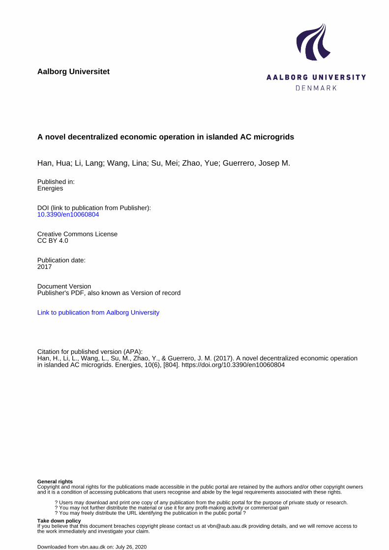
where Pi,m0 and Pi,mt are two active power points, from which hi(Pi) of the ith DG starts to changeaccording to (13). Pi,m0 is a value close to Pi,min but larger than Pi,min. Pi,mt is a value close to Pi,max butsmaller than Pi,max. The OSO and SSO modes of the MG are connected at ( fumax, Pi,m0) and ( fumin, Pi,mt).gi,m0(Pi) and gi,mt(Pi) are the functions of Pi, the design principles of which are illustrated in detail asfollows.
An example of the P-f characteristic curves of the DGs under the modified droop control scheme in(12) and (13) is shown in Figure 4. Take DG2 for instance. When locates in [P2,min,P2,m0] or [P2,mt,P2,max]required by the economic operation, the droop curve of DG2 should be modified as g2,m0(P2) org2,mt(P2), as shown in Figure 4a,b, respectively.
Energies 2017, 10, 804 6 of 18
, 0 ,min , 0
, 0 ,
, , ,max
,
/ ,
,
i m i i i i m
i i i i i i m i i mt
i mt i i mt i i
g P P P P
h P C P P P P P
g P P P P
(13)
where , 0i mP and ,i mtP are two active power points, from which i ih P of the ith DG starts to change according to (13). , 0i mP is a value close to ,miniP but larger than ,miniP . ,i mtP is a value close to ,maxiP but smaller than ,maxiP . The OSO and SSO modes of the MG are connected at ( maxuf , , 0i mP ) and
( minuf , ,i mtP ). , 0i m ig P and ,i mt ig P are the functions of iP , the design principles of which are illustrated in detail as follows.
An example of the P-f characteristic curves of the DGs under the modified droop control scheme in (12) and (13) is shown in Figure 4. Take DG2 for instance. When locates in [ min,2P , 0,2 mP ] or [ mtP ,2 , max,2P ] required by the economic operation, the droop curve of DG2 should be modified as
)( 20,2 Pg m or )( 2,2 Pg mt, as shown in Figure 4a,b, respectively.
Figure 4. P-f characteristic curves of the distributed generations (DGs): (a) a zoomed-in portion of P-f characteristic curves of DG2 when 2P locates in the range of [ 2,minP , 2, 0mP ]; (b) a zoomed-in portion of P-f characteristic curves of DG2 when 2P locates in the range of [ 2,mtP , 2,maxP ]; and (c) P-f
characteristic curves of the DGs under the proposed scheme.
The design of , 0i m ig P and ,i mt ig P should satisfy the following requirements:
(1) i ih P shall be smooth and continuous in the range of [ ,miniP , ,maxiP ], especially function i ih P should be continues at the connecting points , 0i mP and ,i mtP .
(2) In order to obtain synchronous operation within DGs’ capacity limitations, i ih P should start from (Pi,min, fmax) and end at (Pi,max, fmin), namely gi,m0(Pi = Pi,max) = fmax, gi,mt(Pi = Pi,max) = fmin.
(3) The droop coefficients should satisfy the stability constraints of the MG, i.e., , , 0 max0 i mt i i i m i idg P dP dg P dP m . maxm is the permissible maximum droop coefficient
determined by the technical conditions of DGs and also by the requirement of a broad stability domain of the MG.
According to the above requirements, the mathematical descriptions of design principles of , 0i m ig P and ,i mt ig P are as follows:
2,mtP
maxm
2, 0 2mg Pmaxm
2, 0mP
2, 2mtg P
3f
2f1f
maxuf
minuf
Figure 4. P-f characteristic curves of the distributed generations (DGs): (a) a zoomed-in portion of P-fcharacteristic curves of DG2 when P2 locates in the range of [P2,min, P2,m0]; (b) a zoomed-in portion ofP-f characteristic curves of DG2 when P2 locates in the range of [P2,mt, P2,max]; and (c) P-f characteristiccurves of the DGs under the proposed scheme.
The design of gi,m0(Pi) and gi,mt(Pi) should satisfy the following requirements:
(1) hi(Pi) shall be smooth and continuous in the range of [Pi,min, Pi,max], especially function hi(Pi)
should be continues at the connecting points Pi,m0 and Pi,mt.(2) In order to obtain synchronous operation within DGs’ capacity limitations, hi(Pi) should start
from (Pi,min, fmax) and end at (Pi,max, fmin), namely gi,m0(Pi = Pi,max) = fmax, gi,mt(Pi = Pi,max) = fmin.(3) The droop coefficients should satisfy the stability constraints of the MG, i.e., 0 <
dgi,mt(Pi)/dPi( dgi,m0(Pi)/dPi) ≤ mmax. mmax is the permissible maximum droop coefficientdetermined by the technical conditions of DGs and also by the requirement of a broad stabilitydomain of the MG.

Energies 2017, 10, 804 7 of 18
According to the above requirements, the mathematical descriptions of design principles ofgi,m0(Pi) and gi,mt(Pi) are as follows:
limPi→P+
i,mt
γ∂Ci(Pi)/∂Pi− (γ∂Ci(Pi)/∂Pi)|Pi,mtPi−Pi,mt
= limPi→P−i,mt
gi,mt(Pi)−gi,mt(Pi,mt)Pi−Pi,mt
(γ∂Ci(Pi)/∂Pi)|Pi,mt= gi,mt(Pi,mt)
gi,mt(Pi = Pi,max) = fmin
0 < dgi,mt(Pi)/dPi ≤ mmax
(14)
lim
Pi→P+i,m0
gi,m0(Pi)−gi,m0(Pi,m0)Pi−Pi,m0
= limPi→P−i,m0
γ∂Ci(Pi)/∂Pi− (γ∂Ci(Pi)/∂Pi)|Pi,m0Pi−Pi,m0
(γ∂Ci(Pi)/∂Pi)|Pi,m0= gi,m0(Pi,m0)
gi,m0(Pi = Pi,min) = fmax
0 < dgi,m0(Pi)/dPi ≤ mmax
(15)
It is obvious that, large mmax is favourable for economic operation for MG. But an unreasonablemmax may lead to the power-angle oscillation and even cause instability in the MG [38]. Therefore,mmax should be selected as a tradeoff between economy and stability factors. In this paper, mmax is setat 5Hz/p.u.
The optimal Pi,m0, Pi,mt, gi,m0(Pi) and gi,mt(Pi) can be designed through functional analysis methodunder the constraints of (14) and (15). For simplicity at the same time without losing effectiveness,the piecewise parabolic fitting method is adopted in this paper. For example, in our work, Pi,m0was set to (Pi,min + 0.08 Pi,max), while Pi,mt was set to 0.9 Pi,max. Figure 4 shows the P-f characteristiccurves obtained by the piecewise parabolic fitting method, which are used in the simulation andexperiment work.
5. Small Signal Analysis
To investigate the stability of the MG, the small-signal analysis method [39,40] is applied. Withoutloss of generality, the equivalent circuit of the MG composed of n DGs shown in Figure 5 is studied.In Figure 5, Viejδi is the terminal voltage of the ith DG, Vxejδx is the voltage of the common bus, δi andδx are the phase angles of the corresponding voltages, yi is the equivalent admittance between the ith
DG and the common bus, and yx is the equivalent admittance of the comprehensive load.
Energies 2017, 10, 804 7 of 18
,
, ,
,
, , ,
, ,
, ,
, ,max min
, max
/ /lim lim
/
0
i mt
i i mt i i mt
i mt
i i i i i i P i mt i i mt i mt
P P P Pi i mt i i mt
i i i i mt i mtP
i mt i i
i mt i i
C P P C P P g P g P
P P P P
C P P g P
g P P f
dg P dP m
(14)
, 0
, 0 , 0
, 0
, 0 , 0 , 0
, 0 , 0
, 0 , 0
, 0 ,min max
, 0 max
/ /lim lim
/
0
i m
i i m i i m
i m
i i i i i i Pi m i i m i m
P P P Pi i m i i m
i i i i m i mP
i m i i
i m i i
C P P C P Pg P g P
P P P P
C P P g P
g P P f
dg P dP m
(15)
It is obvious that, large maxm is favourable for economic operation for MG. But an unreasonable
maxm may lead to the power-angle oscillation and even cause instability in the MG [38]. Therefore,
maxm should be selected as a tradeoff between economy and stability factors. In this paper, maxm is set at 5Hz . .p u
The optimal , 0i mP , ,i mtP , , 0i m ig P and ,i mt ig P can be designed through functional analysis method under the constraints of (14) and (15). For simplicity at the same time without losing effectiveness, the piecewise parabolic fitting method is adopted in this paper. For example, in our work, , 0i mP was set to ,min ,max0.08i iP P , while ,i mtP was set to ,max0.9 iP . Figure 4 shows the P-f
characteristic curves obtained by the piecewise parabolic fitting method, which are used in the simulation and experiment work.
5. Small Signal Analysis
To investigate the stability of the MG, the small-signal analysis method [39,40] is applied. Without loss of generality, the equivalent circuit of the MG composed of n DGs shown in Figure 5 is studied. In Figure 5, ij
iV e is the terminal voltage of the ith DG, xj
xV e is the voltage of the common
bus, i and x are the phase angles of the corresponding voltages, iy is the equivalent admittance between the ith DG and the common bus, and xy is the equivalent admittance of the comprehensive load.
11jV e nj
nV e
22jV e
xjxV e
1y ny
2yxy
Figure 5. Equivalent circuit of an n-DG MG.
5.1. Small Signal Analysis for the Necessity of Modifications
Based on Kirchhoff current laws, the common bus voltage can be expressed as:
1
x i
nj j
x i ii
V e yV e
(16)
where:
Figure 5. Equivalent circuit of an n-DG MG.
5.1. Small Signal Analysis for the Necessity of Modifications
Based on Kirchhoff current laws, the common bus voltage can be expressed as:
Vxejδx =n
∑i=1
y′iViejδi (16)
where:y′i =
yi
yx +n∑
i=1yi
(17)

Energies 2017, 10, 804 8 of 18
and y′i can be rewritten as:y′i =
∣∣Y′i ∣∣ejθi (18)
where∣∣Y′i ∣∣ and θi are the modulus and angle of y′i, respectively.
The output active power and reactive power of the ith DG is defined as [41]:
Pi =Vi
R2i + X2
i[Ri(Vi −Vx cos δix) + XiVx sin δix] (19)
Qi =Vi
R2i + X2
i[−RiVi sin δix + Xi(Vi −Vx cos δix)] (20)
where δix = δi − δx is the phase angle difference between Viejδi and Vxejδx .With yi = 1/(Ri + jXi), Gi =
RiR2
i +X2i, Bi = − Xi
R2i +X2
i, and (16)–(20), it is easy to obtain the new
expressions of the output active and reactive power of the ith DG without the appearance of Vx and δx:
Pi = GiV2i − GiVi
n
∑j=1
Vj
∣∣∣Y′j ∣∣∣ cos(δi − δj − θj
)− BiVi
n
∑j=1
Vj
∣∣∣Y′j ∣∣∣ sin(δi − δj − θj
)(21)
Qi = −BiV2i + BiVi
n
∑j=1
Vj
∣∣∣Y′j ∣∣∣ cos(δi − δj − θj
)− GiVi
n
∑j=1
Vj
∣∣∣Y′j ∣∣∣ sin(δi − δj − θj
)(22)
In both high and medium voltage systems, Ri Xi. Consequently, Gi Bi. Compared with Xiand Bi respectively, Ri and Gi can be neglected. As a result, (21) and (22) can be simplified as:
Pi =ViXi
n
∑j=1
Vj
∣∣∣Y′j ∣∣∣ sin(δi − δj − θj
)(20)
Qi =V2
iXi− Vi
Xi
n
∑j=1
Vj
∣∣∣Y′j ∣∣∣ cos(δi − δj − θj
)(21)
Suppose that the output frequency reference is tracked by the ith DG without the steady-stateerror. Then the proposed droop control scheme in (12) can be written as follows:
ωi = ωmax − 2πhi(Pi) (25)
where ωi is the output angular frequency of the ith DG, ωi = 2π f ∗i .Assume that ωs is the MG synchronous operation angle frequency in the steady state. Let
δs =∫
ωsdt, and denote δi = δi − δs, then (25) can be rewritten as:
.δi = ωmax −ωs − 2πhi(Pi) (26)
Since P-f has a much slower dynamic characteristic compared with the voltage dynamics, thevoltage dynamics can be neglected when the P-f relationship is analyzed. Linearization of (23) and (26)near the equilibrium point in the Laplace domain yields:
∆Pi =ViXi
n
∑j=1
Vj
∣∣∣Y′j ∣∣∣ cos(
δoi − δo
j − θj
)(∆δi − ∆δj
)(27)
∆.δi = −2πdPo
i ∆Pi (28)
dPoi =
∂hi(Pi)
∂Pi
∣∣∣∣Po
i
(29)

Energies 2017, 10, 804 9 of 18
where ‘’ is the corresponding value around the equilibrium point. By substituting (27) into (28), andneglecting δo
i − δoj , we can get:
∆.δi = −2πdPo
iViXi
n
∑j=1,j 6=i
Vj
∣∣∣Y′j ∣∣∣ cos(−θj
)(∆δi − ∆δj
)(30)
Expressing (30) in matrix form:.X = AX (31)
where X =[
∆δ1 · · · ∆δn
]T, A = −
[aij], aii = 2πdPo
iViXi
n∑
j=1,j 6=iVj
∣∣∣Y′j ∣∣∣ cos(−θj
),
aij = −2πdPoi
ViXi
Vj
∣∣∣Y′j ∣∣∣ cos(−θj
).
Obviously, aii +n∑
i 6=j,j=1aij = 0. If aii > 0, −A is a Laplacian matrix, the eigenvalues of A are in
the left half-plane [42]. Consequently, the related system is stable. In order to ensure aii > 0, thereshould be:
2πdPoi
ViXi
n
∑j=1
Vj
∣∣∣Y′j ∣∣∣ cos(−θj
)> 0 (32)
Due to the fact that 0 < θj < 90o, cos(−θj
)> 0. In order to ensure (32), there should be dPo
i > 0.To ensure dPo
i > 0, (12) should be a strictly monotonically decreasing function on [Pi,min, Pi,max].If not, converting the nonmonotonic parts into monotonic manner is recommended for stability reasons.Without loss of generality, the conditions mentioned above can also be applied to guide the constructionof P-f droop scheme for other objectives.
5.2. Root-Locus Analysis for the Proposed Scheme in the Considered Microgrid
The resistor-inductance line and output filter are considered to depict the root locus diagrams.And the filtered active power Pi f and reactive power Qi f with the output filter can be rewritten as:
Pi f = Piωc
s + ωc⇒
.Pi f =
(Pi − Pi f
)ωc (33)
Qi f = Qiωc
s + ωc⇒
.Qi f =
(Qi −Qi f
)ωc (34)
where ωcs+ωc
is the s-domain transfer function of the output filter, ωc is the cutoff frequency of the filterand the same ωc is assumed for all DGs.
The small-signal model of (23), (24), (26), (33) and (34) around the stable operating point is givenas follows: .
Y = BY (35)
Y =[
∆P1 f · · · ∆Pn f ∆Q1 f · · · ∆Qn f ∆δ1 · · · ∆δn
]T(36)
B =
−ωcI −ωcTpV ωcTpδ0n×n −ωcTqV −ωcI ωcTqδ0n×n 0n×n −TP
(37)
where:
TpV =
w1
∂P1∂V1
· · · wn∂P1∂Vn
.... . .
...w1
∂Pn∂V1
· · · wn∂Pn∂Vn
; Tpδ =
∂P1∂δ1
· · · ∂P1∂δn
.... . .
...∂Pn∂δ1
· · · ∂Pn∂δn
; TqV =
w1
∂Q1∂V1
· · · wn∂Q1∂Vn
.... . .
...w1
∂Qn∂V1
· · · wn∂Qn∂Vn
;
Energies 2017, 10, 804 10 of 18
Tqδ =
∂Q1∂δ1
· · · ∂Q1∂δn
.... . .
...∂Qn∂δ1
· · · ∂Qn∂δn
; I = diag[
1 · · · 1]
n×n; TP = diag
[∂h1(P1 f )
∂P1 f· · · ∂hn(Pn f )
∂Pn f
]n×n
;
and wi is Q-V droop coefficients.To test the stability of the proposed droop control scheme, the root-locus method is used for the
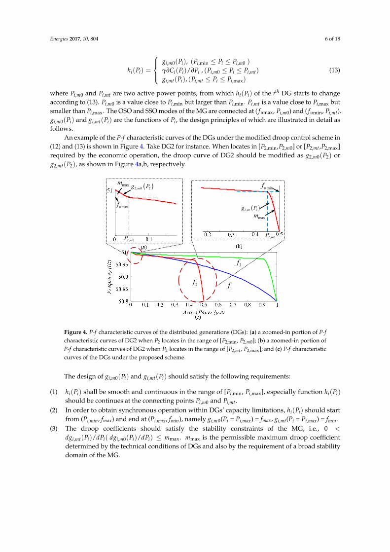
considered MG shown in Figure 2. And resistance-inductance load is assumed. The root locus diagramby changing the load resistance and the line coupling inductance is studied.
Figure 6 shows the root locus diagram with the load resistance changing from 50 Ω to 100 Ω(i.e., PLD changes from 1.08 p.u. to 2.16 p.u., assuming the voltage of the common bus is invariant),while the load inductance LL is set 6 mH, and the equivalent line coupling impedance Zi = Ri + jωiLibetween the ith DG and the common bus is set Ri = 0.12 Ω, Li = 1.5 mH. In Figure 6, there is asingle eigenvalue at zero corresponding to rotational symmetry, as also depicted in [43]. And the resteigenvalues are in the left half-plane. Thus the system is stable.
Energies 2017, 10, 804 10 of 18
1 11
1
11
nn
n nn
n
P Pw w
V V
P Pw w
V V
pVT ;
1 1
1
1
n
n n
n
P P
P P
pδT ;
1 11
1
11
nn
n nn
n
Q Qw w
V V
Q Qw w
V V
qVT ;
1 1
1
1
n
q
n n
n
Q Q
Q Q
δT ; 1 1n n
diag
I ; 1 1
1
f n nf
f nfn n
h P h Pdiag
P P
PT ;
and iw is Q-V droop coefficients. To test the stability of the proposed droop control scheme, the root-locus method is used for the
considered MG shown in Figure 2. And resistance-inductance load is assumed. The root locus diagram by changing the load resistance and the line coupling inductance is studied.
Figure 6 shows the root locus diagram with the load resistance changing from 50 Ω to 100 Ω (i.e., LDP changes from 1.08 p.u. to 2.16 p.u., assuming the voltage of the common bus is invariant), while the load inductance LL is set 6 mH, and the equivalent line coupling impedance
i i i iZ R j L between the ith DG and the common bus is set 0.12iR , 1.5 mHiL . In Figure 6, there is a single eigenvalue at zero corresponding to rotational symmetry, as also depicted in [43]. And the rest eigenvalues are in the left half-plane. Thus the system is stable.
Figure 7 shows the root locus diagram as iL decreases from 3 mH to 0.1 mH, while 0.12iR , 100LR 6 mHLL . In this case, there is also an eigenvalue at zero, as also depicted in [43]. When
the value of Xi decreases, the poles move from the left half plane to the right half plane. Finally the system loses its stability. In this example, the stable operation can be ensured with the proposed scheme when the line coupling inductance including the output filter is more than 0.14 mH. That is to say, the total line coupling inductance shouldn’t be too small for stability reason, which is often ignored in most literatures.
Figure 6. Root locus as the load resistance increases from 50 Ω to 100 Ω.
Figure 7. Root locus by decreasing the line coupling inductance.
Figure 6. Root locus as the load resistance increases from 50 Ω to 100 Ω.
Figure 7 shows the root locus diagram as Li decreases from 3 mH to 0.1 mH, while Ri = 0.12 Ω,RL = 100 Ω LL = 6 mH. In this case, there is also an eigenvalue at zero, as also depicted in [43].When the value of Xi decreases, the poles move from the left half plane to the right half plane. Finallythe system loses its stability. In this example, the stable operation can be ensured with the proposedscheme when the line coupling inductance including the output filter is more than 0.14 mH. That isto say, the total line coupling inductance shouldn’t be too small for stability reason, which is oftenignored in most literatures.
Energies 2017, 10, 804 10 of 18
1 11
1
11
nn
n nn
n
P Pw w
V V
P Pw w
V V
pVT ;
1 1
1
1
n
n n
n
P P
P P
pδT ;
1 11
1
11
nn
n nn
n
Q Qw w
V V
Q Qw w
V V
qVT ;
1 1
1
1
n
q
n n
n
Q Q
Q Q
δT ; 1 1n n
diag
I ; 1 1
1
f n nf
f nfn n
h P h Pdiag
P P
PT ;
and iw is Q-V droop coefficients. To test the stability of the proposed droop control scheme, the root-locus method is used for the
considered MG shown in Figure 2. And resistance-inductance load is assumed. The root locus diagram by changing the load resistance and the line coupling inductance is studied.
Figure 6 shows the root locus diagram with the load resistance changing from 50 Ω to 100 Ω (i.e., LDP changes from 1.08 p.u. to 2.16 p.u., assuming the voltage of the common bus is invariant), while the load inductance LL is set 6 mH, and the equivalent line coupling impedance
i i i iZ R j L between the ith DG and the common bus is set 0.12iR , 1.5 mHiL . In Figure 6, there is a single eigenvalue at zero corresponding to rotational symmetry, as also depicted in [43]. And the rest eigenvalues are in the left half-plane. Thus the system is stable.
Figure 7 shows the root locus diagram as iL decreases from 3 mH to 0.1 mH, while 0.12iR , 100LR 6 mHLL . In this case, there is also an eigenvalue at zero, as also depicted in [43]. When
the value of Xi decreases, the poles move from the left half plane to the right half plane. Finally the system loses its stability. In this example, the stable operation can be ensured with the proposed scheme when the line coupling inductance including the output filter is more than 0.14 mH. That is to say, the total line coupling inductance shouldn’t be too small for stability reason, which is often ignored in most literatures.
Figure 6. Root locus as the load resistance increases from 50 Ω to 100 Ω.
Figure 7. Root locus by decreasing the line coupling inductance. Figure 7. Root locus by decreasing the line coupling inductance.
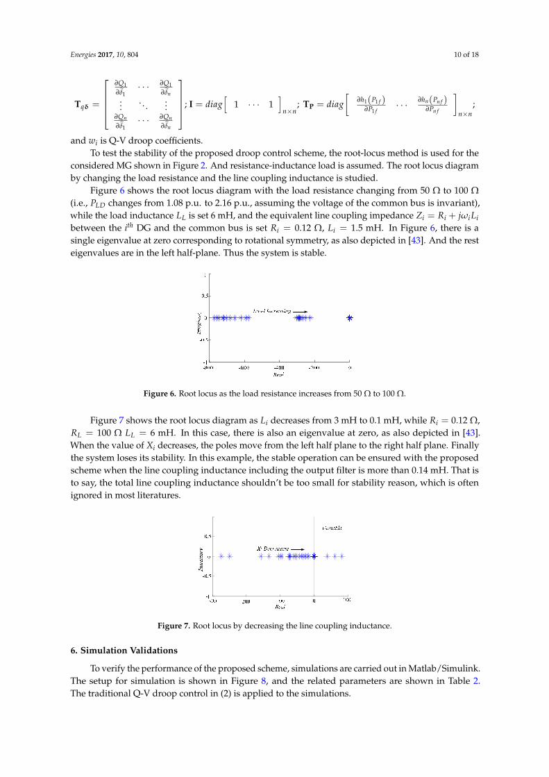
6. Simulation Validations
To verify the performance of the proposed scheme, simulations are carried out in Matlab/Simulink.The setup for simulation is shown in Figure 8, and the related parameters are shown in Table 2.The traditional Q-V droop control in (2) is applied to the simulations.
Energies 2017, 10, 804 11 of 18
Energies 2017, 10, 804 11 of 18
6. Simulation Validations
To verify the performance of the proposed scheme, simulations are carried out in Matlab/Simulink. The setup for simulation is shown in Figure 8, and the related parameters are shown in Table 2. The traditional Q-V droop control in (2) is applied to the simulations.
Figure 8. Scaled-down simulation AC MGs.
Table 2. Parameters for simulation.
Parameter Values Parameter Values
Frequency [50.8, 51] Hz Max ( 2P ) 0.5 p.u.
Voltage [0.95, 1.05] p.u. Max ( 3P ) 1 p.u.
Basic voltage 380 V Max 1 1 1/dC P dP ) 0.563
Basic power 4 kW Max ( 2 2 2/dC P dP ) 0.359
Max ( 1P ) 1 p.u. Max ( 3 3 3/dC P dP ) 0.109
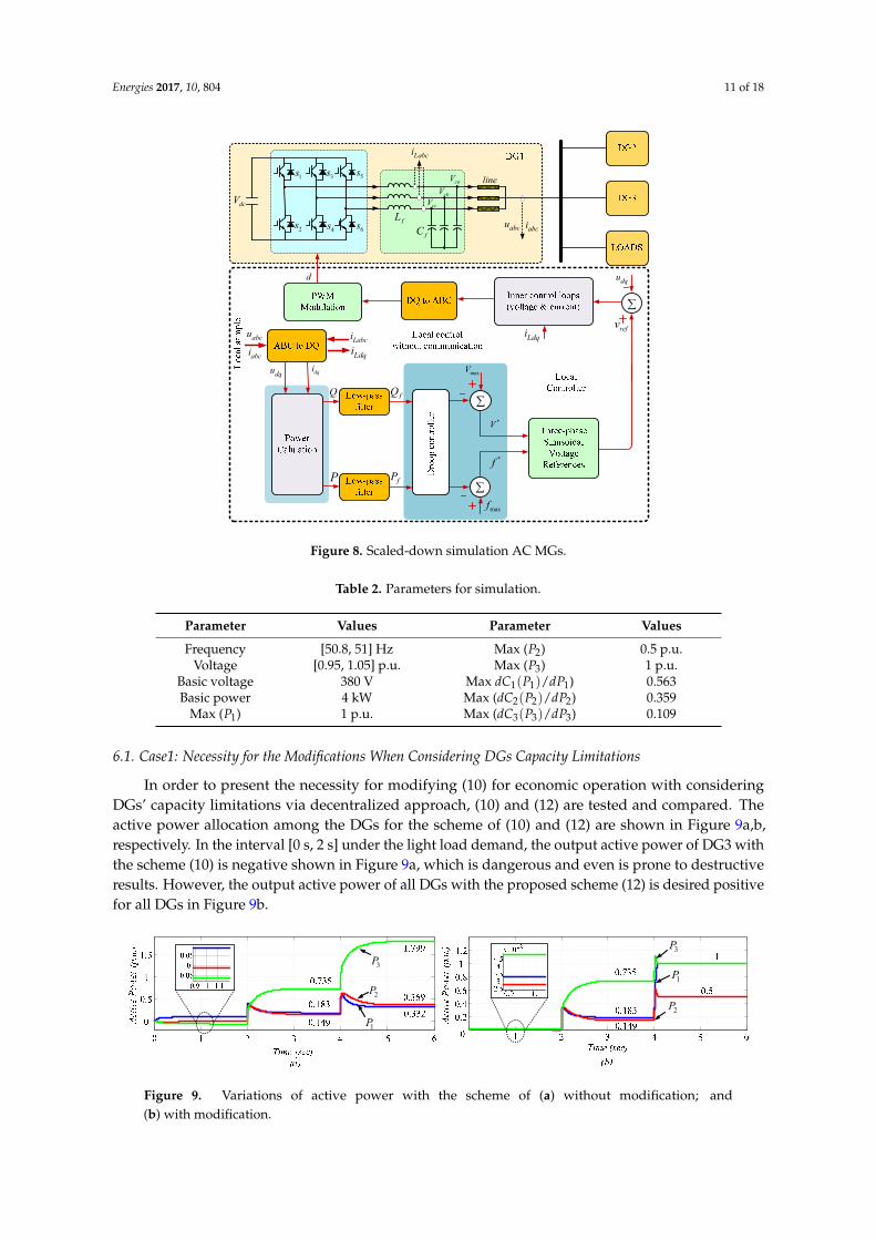
6.1. Case1: Necessity for the Modifications When Considering DGs Capacity Limitations
In order to present the necessity for modifying (10) for economic operation with considering DGs’ capacity limitations via decentralized approach, (10) and (12) are tested and compared. The active power allocation among the DGs for the scheme of (10) and (12) are shown in Figure 9a,b, respectively. In the interval [0 s, 2 s] under the light load demand, the output active power of DG3 with the scheme (10) is negative shown in Figure 9a, which is dangerous and even is prone to destructive results. However, the output active power of all DGs with the proposed scheme (12) is desired positive for all DGs in Figure 9b.
In the interval [2 s, 4 s] under the medium load demand, the output active power of all DGs with the droop scheme (10) and (12) are same, which is related to OSO conditions. When a full load appears in the interval [4 s, 6 s], the output of DG3 with (10) is 1.799 p.u. (It exceeds its maximum capacity 1 p.u.), which is not permissible. However, the proposed droop scheme (12) could control all DGs in their maximum capacity ( 1 1 . .P p u , 2 0.5 . .P p u , 3 1 . .P p u ).
1s 3s 5s
2s 4s 6sfC
fL
caV
cbV
ccVdcV
line
abcu abci
Labci
*V
*f
maxf
maxVdqi
refv
abcu
abci
dqu
dqud
Labci
LdqiLdqi
P
Q
fP
fQ
Figure 8. Scaled-down simulation AC MGs.
Table 2. Parameters for simulation.
Parameter Values Parameter Values
Frequency [50.8, 51] Hz Max (P2) 0.5 p.u.Voltage [0.95, 1.05] p.u. Max (P3) 1 p.u.
Basic voltage 380 V Max dC1(P1)/dP1) 0.563Basic power 4 kW Max (dC2(P2)/dP2) 0.359
Max (P1) 1 p.u. Max (dC3(P3)/dP3) 0.109
6.1. Case1: Necessity for the Modifications When Considering DGs Capacity Limitations
In order to present the necessity for modifying (10) for economic operation with consideringDGs’ capacity limitations via decentralized approach, (10) and (12) are tested and compared. Theactive power allocation among the DGs for the scheme of (10) and (12) are shown in Figure 9a,b,respectively. In the interval [0 s, 2 s] under the light load demand, the output active power of DG3 withthe scheme (10) is negative shown in Figure 9a, which is dangerous and even is prone to destructiveresults. However, the output active power of all DGs with the proposed scheme (12) is desired positivefor all DGs in Figure 9b.
Energies 2017, 10, 804 12 of 18
Accordingly, the simulation results verified that the proposed droop scheme (12) could protect generators from being destroyed due to overloading or negative power impact.
Figure 9. Variations of active power with the scheme of (a) without modification; and (b) with modification.
6.2. Case 2: Economy Comparisons between the Proposed P-f Scheme and the Interior Point Method
For comparison, the economical operation solutions through the interior point method [44] are depicted in Figure 10a. The corresponding TAGC of the MG is shown in Figure 10b. As shown in Figure 10a, in case when the DG active power output reaches its maximum value as load increases,
0oidP . Then 0o
idP is not satisfied, which is unfavourable for system stability. Thus, modifications are necessary for stability reasons. Besides, in order to achieve the optimal economic operation, the centralized controllers with communications are usually needed.
Figure 10. Power allocation results (a) power allocation among DGs through the interior point method; (b) total active generation cost (TAGC) of the interior point method; (c) power allocation among DGs through the proposed droop control scheme; (d) TAGC of the proposed droop control scheme.
Under the same setup, the economical operation solutions of the proposed droop control scheme using (12) are shown in Figure 10c. Although there are some subtle distinctions between Figure 10a,c, the distinctions of TAGC under the two schemes as shown in Figure 10d is not obvious. In most cases, the TAGC of the proposed scheme (12) are in good agreement with that in Figure 10b. Based on the simulation results, it is verified that the proposed droop control scheme (12) could achieve satisfactory economic operations even in the presence of capacity limitations.
6.3. Case 3: Performance of the Proposed P-f Scheme
To verify the performance of the proposed P-f scheme, simulation is implemented as load step changes at 2 s and 4 s shown in Figure 11a. When the MG gets into the steady state, the frequency
1P
3P
2P
3P
1P
2P
3P
2P
1P
3P
2P
1P
Figure 9. Variations of active power with the scheme of (a) without modification; and(b) with modification.

Energies 2017, 10, 804 12 of 18
In the interval [2 s, 4 s] under the medium load demand, the output active power of all DGs withthe droop scheme (10) and (12) are same, which is related to OSO conditions. When a full load appearsin the interval [4 s, 6 s], the output of DG3 with (10) is 1.799 p.u. (It exceeds its maximum capacity1 p.u.), which is not permissible. However, the proposed droop scheme (12) could control all DGs intheir maximum capacity (P1 = 1 p.u., P2 = 0.5 p.u., P3 = 1 p.u.).
Accordingly, the simulation results verified that the proposed droop scheme (12) could protectgenerators from being destroyed due to overloading or negative power impact.
6.2. Case 2: Economy Comparisons between the Proposed P-f Scheme and the Interior Point Method
For comparison, the economical operation solutions through the interior point method [44] aredepicted in Figure 10a. The corresponding TAGC of the MG is shown in Figure 10b. As shown inFigure 10a, in case when the DG active power output reaches its maximum value as load increases,dPo
i = 0. Then dPoi > 0 is not satisfied, which is unfavourable for system stability. Thus, modifications
are necessary for stability reasons. Besides, in order to achieve the optimal economic operation, thecentralized controllers with communications are usually needed.
Energies 2017, 10, 804 12 of 18
Accordingly, the simulation results verified that the proposed droop scheme (12) could protect generators from being destroyed due to overloading or negative power impact.
Figure 9. Variations of active power with the scheme of (a) without modification; and (b) with modification.
6.2. Case 2: Economy Comparisons between the Proposed P-f Scheme and the Interior Point Method
For comparison, the economical operation solutions through the interior point method [44] are depicted in Figure 10a. The corresponding TAGC of the MG is shown in Figure 10b. As shown in Figure 10a, in case when the DG active power output reaches its maximum value as load increases,
0oidP . Then 0o
idP is not satisfied, which is unfavourable for system stability. Thus, modifications are necessary for stability reasons. Besides, in order to achieve the optimal economic operation, the centralized controllers with communications are usually needed.
Figure 10. Power allocation results (a) power allocation among DGs through the interior point method; (b) total active generation cost (TAGC) of the interior point method; (c) power allocation among DGs through the proposed droop control scheme; (d) TAGC of the proposed droop control scheme.
Under the same setup, the economical operation solutions of the proposed droop control scheme using (12) are shown in Figure 10c. Although there are some subtle distinctions between Figure 10a,c, the distinctions of TAGC under the two schemes as shown in Figure 10d is not obvious. In most cases, the TAGC of the proposed scheme (12) are in good agreement with that in Figure 10b. Based on the simulation results, it is verified that the proposed droop control scheme (12) could achieve satisfactory economic operations even in the presence of capacity limitations.
6.3. Case 3: Performance of the Proposed P-f Scheme
To verify the performance of the proposed P-f scheme, simulation is implemented as load step changes at 2 s and 4 s shown in Figure 11a. When the MG gets into the steady state, the frequency
1P
3P
2P
3P
1P
2P
3P
2P
1P
3P
2P
1P
Figure 10. Power allocation results (a) power allocation among DGs through the interior point method;(b) total active generation cost (TAGC) of the interior point method; (c) power allocation among DGsthrough the proposed droop control scheme; (d) TAGC of the proposed droop control scheme.
Under the same setup, the economical operation solutions of the proposed droop control schemeusing (12) are shown in Figure 10c. Although there are some subtle distinctions between Figure 10a,c,the distinctions of TAGC under the two schemes as shown in Figure 10d is not obvious. In most cases,the TAGC of the proposed scheme (12) are in good agreement with that in Figure 10b. Based on thesimulation results, it is verified that the proposed droop control scheme (12) could achieve satisfactoryeconomic operations even in the presence of capacity limitations.
6.3. Case 3: Performance of the Proposed P-f Scheme
To verify the performance of the proposed P-f scheme, simulation is implemented as load stepchanges at 2 s and 4 s shown in Figure 11a. When the MG gets into the steady state, the frequencyconverges to a constant as shown in Figure 11b. Figure 11c shows the behavior of hi(Pi) during thetransient process. And active power allocation among DGs through the proposed droop controlscheme is shown in Figure 11d. The simulation results with the proposed scheme are in accordancewith the theoretical results as shown in Figure 10a, the OSO operation is obtained in the first andsecond interval, i.e., 0–2 s and 2–4 s, respectively. The SSO operation is realized in the third interval,i.e., 4–6 s, as a tradeoff between economy and stability.

Energies 2017, 10, 804 13 of 18
Energies 2017, 10, 804 13 of 18
converges to a constant as shown in Figure 11b. Figure 11c shows the behavior of i ih P during the transient process. And active power allocation among DGs through the proposed droop control scheme is shown in Figure 11d. The simulation results with the proposed scheme are in accordance with the theoretical results as shown in Figure 10a, the OSO operation is obtained in the first and second interval, i.e., 0–2 s and 2–4 s, respectively. The SSO operation is realized in the third interval, i.e., 4–6 s, as a tradeoff between economy and stability.
From the simulation results, it is verified that the proposed P-f scheme does very well in response to the step change of the load. The frequency could be controlled within the allowable ranges. And all the DG active power limitations are not conflicted.
Figure 11. Variations of (a) loads; (b) frequency; (c) i ih P ; and (d) active power output of DGs.
6.4. Case 4: Plug and Play Capability of the Proposed P-f Scheme
In this case, the proposed P-f scheme is implemented under a certain load, when DG3 is suddenly lost at 2 s. From the simulation result in Figure 12, the load could be shared automatically among the rest available DGs according to their economic droop curves. Therefore, it is verified that the proposed P-f scheme holds the capability of plug and play, while maintaining the economical allocation of the load.
Figure 12. Variations of active power with losing DG3.
7. Experimental Results
A MG experimental prototype was built to verify the effectiveness of the proposed P-f scheme, as shown in Figure 13. Limited by the experimental conditions, a MG consisting of two DGs was tested. The two DGs are realized utilizing single phase voltage source inverters, which are controlled by digital signal processors (TMS320f28335) with a sampling rate at 12.8 kHz. The coefficients of the DGs’ generation cost functions are as listed in Table 1. And the experimental parameters are shown
1P2P
3P
2f 1f
3f
1 1h P
2 2h P
3 3h P
1P
2P
3P
Figure 11. Variations of (a) loads; (b) frequency; (c) hi(Pi); and (d) active power output of DGs.
From the simulation results, it is verified that the proposed P-f scheme does very well in responseto the step change of the load. The frequency could be controlled within the allowable ranges. And allthe DG active power limitations are not conflicted.
6.4. Case 4: Plug and Play Capability of the Proposed P-f Scheme
In this case, the proposed P-f scheme is implemented under a certain load, when DG3 is suddenlylost at 2 s. From the simulation result in Figure 12, the load could be shared automatically among therest available DGs according to their economic droop curves. Therefore, it is verified that the proposedP-f scheme holds the capability of plug and play, while maintaining the economical allocation ofthe load.
Energies 2017, 10, 804 13 of 18
converges to a constant as shown in Figure 11b. Figure 11c shows the behavior of i ih P during the transient process. And active power allocation among DGs through the proposed droop control scheme is shown in Figure 11d. The simulation results with the proposed scheme are in accordance with the theoretical results as shown in Figure 10a, the OSO operation is obtained in the first and second interval, i.e., 0–2 s and 2–4 s, respectively. The SSO operation is realized in the third interval, i.e., 4–6 s, as a tradeoff between economy and stability.
From the simulation results, it is verified that the proposed P-f scheme does very well in response to the step change of the load. The frequency could be controlled within the allowable ranges. And all the DG active power limitations are not conflicted.
Figure 11. Variations of (a) loads; (b) frequency; (c) i ih P ; and (d) active power output of DGs.
6.4. Case 4: Plug and Play Capability of the Proposed P-f Scheme
In this case, the proposed P-f scheme is implemented under a certain load, when DG3 is suddenly lost at 2 s. From the simulation result in Figure 12, the load could be shared automatically among the rest available DGs according to their economic droop curves. Therefore, it is verified that the proposed P-f scheme holds the capability of plug and play, while maintaining the economical allocation of the load.
Figure 12. Variations of active power with losing DG3.
7. Experimental Results
A MG experimental prototype was built to verify the effectiveness of the proposed P-f scheme, as shown in Figure 13. Limited by the experimental conditions, a MG consisting of two DGs was tested. The two DGs are realized utilizing single phase voltage source inverters, which are controlled by digital signal processors (TMS320f28335) with a sampling rate at 12.8 kHz. The coefficients of the DGs’ generation cost functions are as listed in Table 1. And the experimental parameters are shown
1P2P
3P
2f 1f
3f
1 1h P
2 2h P
3 3h P
1P
2P
3P
Figure 12. Variations of active power with losing DG3.
7. Experimental Results
A MG experimental prototype was built to verify the effectiveness of the proposed P-f scheme,as shown in Figure 13. Limited by the experimental conditions, a MG consisting of two DGs wastested. The two DGs are realized utilizing single phase voltage source inverters, which are controlledby digital signal processors (TMS320f28335) with a sampling rate at 12.8 kHz. The coefficients of theDGs’ generation cost functions are as listed in Table 1. And the experimental parameters are shown inTable 3. The experiments are carried out in terms of the proposed P-f scheme as the load of the MGchanges. The traditional Q-V droop control in (2) is applied to the experiments.

Energies 2017, 10, 804 14 of 18
Energies 2017, 10, 804 14 of 18
in Table 3. The experiments are carried out in terms of the proposed P-f scheme as the load of the MG changes. The traditional Q-V droop control in (2) is applied to the experiments.
Table 3. Parameters for experiments.
Parameters Value Parameters Value Frequency [50.8, 51] Hz Filter inductor 1 mH
Voltage [0.95, 1.05] p.u. Filter capacitor 20 µF Basic voltage 96V (Line rms) Line 3 inductor 0.6 mH Basic power 400 W Line 1, 2 inductor 0.3 mH
Figure 13. Experimental prototype setup of an AC MG.
7.1. Case 1: Performance of the Proposed P-f scheme with Equally Rated DGs (DG1 and DG3)
In this experimental case, the generation cost function coefficients of the DG1 and DG3, as listed in Table 1, are used to verify the proposed scheme. DG1 and DG3 having equal rated capacity is assumed at 1 p.u. The voltage waveforms on the common bus and the current waveforms of the DGs based on the proposed P-f scheme are shown in Figure 14. The waveforms of the load, frequency, i ih P and active power allocations of DG1 and DG3 based on the proposed P-f scheme are
illustrated in Figure 15. Since the frequency is applied as a carrier in the proposed P-f scheme, i ih P values of all the DGs are equal even when the load changes, as shown in Figure 15c. Due to the difference of the hardware, the disturbance in the red and blue waveforms is different as shown in Figure 15b,c. And the optimal power dispatch is achieved according to their generation cost function, as shown in Figure 15d, while the smooth and stable operation is maintained even with the capacity limitation constraints.
Figure 14. Experimental voltage and current waveforms.
Figure 13. Experimental prototype setup of an AC MG.
Table 3. Parameters for experiments.
Parameters Value Parameters Value
Frequency [50.8, 51] Hz Filter inductor 1 mHVoltage [0.95, 1.05] p.u. Filter capacitor 20 µF
Basic voltage 96V (Line rms) Line 3 inductor 0.6 mHBasic power 400 W Line 1, 2 inductor 0.3 mH
7.1. Case 1: Performance of the Proposed P-f scheme with Equally Rated DGs (DG1 and DG3)
In this experimental case, the generation cost function coefficients of the DG1 and DG3, as listed inTable 1, are used to verify the proposed scheme. DG1 and DG3 having equal rated capacity is assumedat 1 p.u. The voltage waveforms on the common bus and the current waveforms of the DGs based onthe proposed P-f scheme are shown in Figure 14. The waveforms of the load, frequency, hi(Pi) andactive power allocations of DG1 and DG3 based on the proposed P-f scheme are illustrated in Figure 15.Since the frequency is applied as a carrier in the proposed P-f scheme, hi(Pi) values of all the DGs areequal even when the load changes, as shown in Figure 15c. Due to the difference of the hardware, thedisturbance in the red and blue waveforms is different as shown in Figure 15b,c. And the optimalpower dispatch is achieved according to their generation cost function, as shown in Figure 15d, whilethe smooth and stable operation is maintained even with the capacity limitation constraints.
Energies 2017, 10, 804 14 of 18
in Table 3. The experiments are carried out in terms of the proposed P-f scheme as the load of the MG changes. The traditional Q-V droop control in (2) is applied to the experiments.
Table 3. Parameters for experiments.
Parameters Value Parameters Value Frequency [50.8, 51] Hz Filter inductor 1 mH
Voltage [0.95, 1.05] p.u. Filter capacitor 20 µF Basic voltage 96V (Line rms) Line 3 inductor 0.6 mH Basic power 400 W Line 1, 2 inductor 0.3 mH
Figure 13. Experimental prototype setup of an AC MG.
7.1. Case 1: Performance of the Proposed P-f scheme with Equally Rated DGs (DG1 and DG3)
In this experimental case, the generation cost function coefficients of the DG1 and DG3, as listed in Table 1, are used to verify the proposed scheme. DG1 and DG3 having equal rated capacity is assumed at 1 p.u. The voltage waveforms on the common bus and the current waveforms of the DGs based on the proposed P-f scheme are shown in Figure 14. The waveforms of the load, frequency, i ih P and active power allocations of DG1 and DG3 based on the proposed P-f scheme are
illustrated in Figure 15. Since the frequency is applied as a carrier in the proposed P-f scheme, i ih P values of all the DGs are equal even when the load changes, as shown in Figure 15c. Due to the difference of the hardware, the disturbance in the red and blue waveforms is different as shown in Figure 15b,c. And the optimal power dispatch is achieved according to their generation cost function, as shown in Figure 15d, while the smooth and stable operation is maintained even with the capacity limitation constraints.
Figure 14. Experimental voltage and current waveforms. Figure 14. Experimental voltage and current waveforms.
Energies 2017, 10, 804 15 of 18
Energies 2017, 10, 804 15 of 18
Figure 15. Waveforms of (a) the load; (b) frequency; (c) i ih P values; and (d) DGs’ active
power outputs.
7.2. Case 2: Performance of the Proposed P-f Scheme with Unequally Rated DGs (DG2 and DG3)
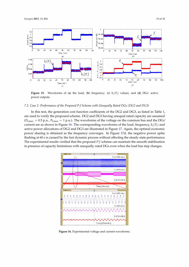
In this test, the generation cost function coefficients of the DG2 and DG3, as listed in Table 1, are used to verify the proposed scheme. DG2 and DG3 having unequal rated capacity are assumed ( 2,max 0.5 . .P p u , 3,max 1 . .P p u ). The waveforms of the voltage on the common bus and the DGs’
current are as shown in Figure 16. The corresponding waveforms of the load, frequency, i ih P and active power allocations of DG2 and DG3 are illustrated in Figure 17. Again, the optimal economic power sharing is obtained as the frequency converges. In Figure 17d, the negative power spike flashing at 60 s is caused by the fast dynamic process without affecting the steady state performance. The experimental results verified that the proposed P-f scheme can maintain the smooth stabilization in presence of capacity limitations with unequally rated DGs even when the load has step changes.
Figure 16. Experimental voltage and current waveforms.
1 1h P
3 3h P1P
3P
Figure 15. Waveforms of (a) the load; (b) frequency; (c) hi(Pi) values; and (d) DGs’ activepower outputs.
7.2. Case 2: Performance of the Proposed P-f Scheme with Unequally Rated DGs (DG2 and DG3)
In this test, the generation cost function coefficients of the DG2 and DG3, as listed in Table 1,are used to verify the proposed scheme. DG2 and DG3 having unequal rated capacity are assumed(P2,max = 0.5 p.u., P3,max = 1 p.u.). The waveforms of the voltage on the common bus and the DGs’current are as shown in Figure 16. The corresponding waveforms of the load, frequency, hi(Pi) andactive power allocations of DG2 and DG3 are illustrated in Figure 17. Again, the optimal economicpower sharing is obtained as the frequency converges. In Figure 17d, the negative power spikeflashing at 60 s is caused by the fast dynamic process without affecting the steady state performance.The experimental results verified that the proposed P-f scheme can maintain the smooth stabilizationin presence of capacity limitations with unequally rated DGs even when the load has step changes.
Energies 2017, 10, 804 15 of 18
Figure 15. Waveforms of (a) the load; (b) frequency; (c) i ih P values; and (d) DGs’ active
power outputs.
7.2. Case 2: Performance of the Proposed P-f Scheme with Unequally Rated DGs (DG2 and DG3)
In this test, the generation cost function coefficients of the DG2 and DG3, as listed in Table 1, are used to verify the proposed scheme. DG2 and DG3 having unequal rated capacity are assumed ( 2,max 0.5 . .P p u , 3,max 1 . .P p u ). The waveforms of the voltage on the common bus and the DGs’
current are as shown in Figure 16. The corresponding waveforms of the load, frequency, i ih P and active power allocations of DG2 and DG3 are illustrated in Figure 17. Again, the optimal economic power sharing is obtained as the frequency converges. In Figure 17d, the negative power spike flashing at 60 s is caused by the fast dynamic process without affecting the steady state performance. The experimental results verified that the proposed P-f scheme can maintain the smooth stabilization in presence of capacity limitations with unequally rated DGs even when the load has step changes.
Figure 16. Experimental voltage and current waveforms.
1 1h P
3 3h P1P
3P
Figure 16. Experimental voltage and current waveforms.

Energies 2017, 10, 804 16 of 18
Energies 2017, 10, 804 16 of 18
Figure 17. Variations of (a) loads; (b) frequency; (c) i ih P ; and (d) DGs active power over time.
8. Conclusions
In this paper, a P-f droop scheme for MGs is proposed to reduce the MG TAGC via a decentralized approach. The sufficient conditions for MG economic operation under the proposed P-f droop method are explored by the small-signal analysis method. Because the implementation of the proposed P-f scheme only needs the local information of each DG, communications are not needed. Therefore, it represents a reliable and low-cost solution. In addition, to deal with the limitations of DGs’ capacity, a modification method is proposed, which guarantees the synchronization and stability of the MGs. Both simulation and experimental results have verified the effectiveness of the proposed scheme.
Acknowledgments: This work was supported by the National Natural Science Foundation of China under Grant No. 61573384, and the Natural Science Foundation of Hunan Province of China under Grant No. 2016JJ1019.
Author Contributions: Lang Li conceived the main idea and wrote the manuscript with guidance from Hua Han and Mei Su. Lina Wang, Yue Zhao and Josep M. Guerrero reviewed the work and gave helpful improvement suggestions.
Conflicts of Interest: The authors declare no conflict of interest.
References
1. Yu, Z.; Ai, Q.; Gong, J.; Piao, L. A novel secondary control for microgrid based on synergetic control of multi-agent system. Energies 2016, 9, 243.
2. Camblong, H.; Etxeberria, A.; Ugartemendia, J.; Curea, O. Gain Scheduling Control of an Islanded Microgrid Voltage. Energies 2014, 7, 4498–4518.
3. Hu, S.-H.; Lee, T.-L.; Kuo, C.-Y.; Guerrero, J.M. A Riding-through Technique for Seamless Transition between Islanded and Grid-Connected Modes of Droop-Controlled Inverters. Energies 2016, 9, 732.
4. Chen, C.; Duan, S.; Cai, T. Smart energy management system for optimal microgrid economic operation. IET Renew. Power Gener. 2011, 5, 258–267.
5. Fei, W.; Duarte, J. Grid-interfacing converter systems with enhanced voltage quality for microgrid application concept and implementation. IEEE Trans. Power Electron. 2011, 26, 3501–3513.
6. Lim, Y.; Kim, H.M.; Kinoshita, T. Distributed load-shedding system for agent-based autonomous microgrid operations. Energies 2014, 7, 385–401.
7. Lu, X.; Wan, J. Modeling and Control of the Distributed Power Converters in a Standalone DC Microgrid. Energies 2016, 9, 217.
8. Lopes, J.P.; Moreira, C.L.; Madureira, A.G. Defining Control Strategies for MicroGrids Islanded Operation. IEEE Trans. Power Syst. 2006, 21, 916–924.
9. Nikmehr, N.; Ravadanegh, S.N. Optimal Power Dispatch of Multi-Microgrids at Future Smart Distribution Grids. IEEE Trans. Smart Grid 2015, 6, 1648–1657.
2 2h P 3 3h P
3P
2P
Figure 17. Variations of (a) loads; (b) frequency; (c) hi(Pi); and (d) DGs active power over time.
8. Conclusions
In this paper, a P-f droop scheme for MGs is proposed to reduce the MG TAGC via a decentralizedapproach. The sufficient conditions for MG economic operation under the proposed P-f droop methodare explored by the small-signal analysis method. Because the implementation of the proposed P-fscheme only needs the local information of each DG, communications are not needed. Therefore, itrepresents a reliable and low-cost solution. In addition, to deal with the limitations of DGs’ capacity,a modification method is proposed, which guarantees the synchronization and stability of the MGs.Both simulation and experimental results have verified the effectiveness of the proposed scheme.
Acknowledgments: This work was supported by the National Natural Science Foundation of China under GrantNo. 61573384, and the Natural Science Foundation of Hunan Province of China under Grant No. 2016JJ1019.
Author Contributions: Lang Li conceived the main idea and wrote the manuscript with guidance fromHua Han and Mei Su. Lina Wang, Yue Zhao and Josep M. Guerrero reviewed the work and gave helpfulimprovement suggestions.
Conflicts of Interest: The authors declare no conflict of interest.
References
1. Yu, Z.; Ai, Q.; Gong, J.; Piao, L. A novel secondary control for microgrid based on synergetic control ofmulti-agent system. Energies 2016, 9, 243. [CrossRef]
2. Camblong, H.; Etxeberria, A.; Ugartemendia, J.; Curea, O. Gain Scheduling Control of an Islanded MicrogridVoltage. Energies 2014, 7, 4498–4518. [CrossRef]
3. Hu, S.-H.; Lee, T.-L.; Kuo, C.-Y.; Guerrero, J.M. A Riding-through Technique for Seamless Transition betweenIslanded and Grid-Connected Modes of Droop-Controlled Inverters. Energies 2016, 9, 732. [CrossRef]
4. Chen, C.; Duan, S.; Cai, T. Smart energy management system for optimal microgrid economic operation.IET Renew. Power Gener. 2011, 5, 258–267. [CrossRef]
5. Fei, W.; Duarte, J. Grid-interfacing converter systems with enhanced voltage quality for microgrid applicationconcept and implementation. IEEE Trans. Power Electron. 2011, 26, 3501–3513.
6. Lim, Y.; Kim, H.M.; Kinoshita, T. Distributed load-shedding system for agent-based autonomous microgridoperations. Energies 2014, 7, 385–401. [CrossRef]
7. Lu, X.; Wan, J. Modeling and Control of the Distributed Power Converters in a Standalone DC Microgrid.Energies 2016, 9, 217. [CrossRef]
8. Lopes, J.P.; Moreira, C.L.; Madureira, A.G. Defining Control Strategies for MicroGrids Islanded Operation.IEEE Trans. Power Syst. 2006, 21, 916–924. [CrossRef]

Energies 2017, 10, 804 17 of 18
9. Nikmehr, N.; Ravadanegh, S.N. Optimal Power Dispatch of Multi-Microgrids at Future Smart DistributionGrids. IEEE Trans. Smart Grid 2015, 6, 1648–1657. [CrossRef]
10. Barklund, E.; Pogaku, N.; Prodanovic, M.; Hernandez-Aramburo, C.; Green, T.C. Energy management inautonomous microgrid using stability-constrained droop control of inverters. IEEE Trans. Power Electron.2008, 23, 2346–2352. [CrossRef]
11. Nutkani, I.U.; Loh, P.; Wang, P.; Blaabjerg, F. Cost-prioritized droop schemes for autonomous AC microgrids.IEEE Trans. Power Electron. 2015, 30, 1109–1119. [CrossRef]
12. Li, J.; Wei, W.; Xiang, J. A Simple Sizing Algorithm for Stand-Alone PV/Wind/Battery Hybrid Microgrids.Energies 2012, 5, 5307–5323. [CrossRef]
13. Song, N.O.; Lee, J.H.; Kim, H.M.; Im, Y.H.; Lee, J.Y. Optimal energy management of multi-microgrids withsequentially coordinated operations. Energies 2015, 8, 8371–8390. [CrossRef]
14. Hussain, A.; Bui, V.-H.; Kim, H.-M. Robust Optimization-Based Scheduling of Multi-Microgrids ConsideringUncertainties. Energies 2016, 9, 278. [CrossRef]
15. Che, L.; Shahidehpour, M. DC Microgrids: Economic Operation and Enhancement of Resilience byHierarchical Control. IEEE Trans. Smart Grid 2014, 5, 2517–2526.
16. Che, L.; Shahidehpour, M.; Alabdulwahab, A.; Al-Turki, Y. Hierarchical Coordination of a CommunityMicrogrid with AC and DC Microgrids. IEEE Trans. Smart Grid 2015, 6, 3042–3051. [CrossRef]
17. Li, C.; De Bosio, F.; Chen, F.; Chaudhary, S.K.; Vasquez, J.C.; Guerrero, J.M. Economic Dispatch for OperatingCost Minimization Under Real-Time Pricing in Droop-Controlled DC Microgrid. IEEE J. Emerg. Sel. Top.Power Electron. 2017, 5, 587–595. [CrossRef]
18. Tsikalakis, A.G.; Hatziargyriou, N.D. Centralized control for optimizing microgrids operation. IEEE Trans.Energy Convers. 2008, 23, 241–248. [CrossRef]
19. Katiraei, F.; Iravani, R.; Hatziargyriou, N.; Dimeas, A. Microgrids management. IEEE Power Energy Mag.2008, 6, 54–65. [CrossRef]
20. Guerrero, J.M.; Chandorkar, M.; Lee, T.-L. Advanced control architectures for intelligent microgrids—Part I:Decentralized and hierarchical control. IEEE Trans. Ind. Electron. 2013, 60, 1254–1262. [CrossRef]
21. Olivares, D.E.; Mehrizi-Sani, A.; Etemadi, A.H. Trends in microgrid control. IEEE Trans. Smart Grid 2014, 5,1905–1919. [CrossRef]
22. Yazdanian, M.; Mehrizi-Sani, A. Distributed control techniques in microgrids. IEEE Trans. Smart Grid 2014, 5,2901–2909. [CrossRef]
23. Zhang, W.; Liu, W.; Wang, X.; Liu, L.; Ferrese, F. Online optimal generation control based on constraineddistributed gradient algorithm. IEEE Trans. Power Syst. 2015, 30, 35–45. [CrossRef]
24. Zhang, Z.; Chow, M.-Y. Convergence analysis of the incremental cost consensus algorithm under differentcommunication network topologies in a smart grid. IEEE Trans. Power Syst. 2012, 27, 1761–1768. [CrossRef]
25. Yang, S.; Tan, S.; Xu, J.-X. Consensus based approach for economic dispatch problem in a smart grid.IEEE Trans. Power Syst. 2013, 28, 4416–4426. [CrossRef]
26. Yan, B.; Wang, B.; Zhu, L. A novel, stable, and economic power sharing scheme for an autonomous microgridin the energy internet. Energies 2015, 8, 12741–12764. [CrossRef]
27. Ahn, C.; Peng, H. Decentralized and real-time power dispatch control for an islanded microgrid supportedby distributed power sources. Energies 2013, 6, 6439–6454. [CrossRef]
28. Cosse, R.E.; Alford, M.D.; Hajiaghajani, M.; Hamilton, E.R. Turbine/generator governor droop/isochronousfundamentals—A graphical approach. In Proceedings of the Petroleum and Chemical Industry Conference,Toronto, ON, Canada, 19–21 September 2011.
29. Jaleeli, N.; VanSlyck, L.S.; Ewart, D.N.; Fink, L.H.; Hoffmann, A.G. Understanding automatic generationcontrol. IEEE Trans. Power Syst. 1992, 7, 1106–1122. [CrossRef]
30. Guerrero, J.M.; Hang, L.; Uceda, J. Control of distributed uninterruptible power supply systems. IEEE Trans.Ind. Electron. 2008, 55, 2845–2859. [CrossRef]
31. Lee, C.T. A new droop control method for the autonomous operation of distributed energy resource interfaceconverters. IEEE Trans. Power Electron. 2013, 28, 1980–1993. [CrossRef]
32. Haddadi, A.; Joos, G. Load sharing of autonomous distribution-level microgrids. In Proceedings of thePower and Energy Society General Meeting, San Diego, CA, USA, 24–29 July 2011.

Energies 2017, 10, 804 18 of 18
33. Mohamed, Y.A.-R.I.; El-Saadany, E.F. Adaptive decentralized droop controller to preserve power sharingstability of paralleled inverters in distributed generation microgrids. IEEE Trans. Power Electron. 2008, 23,2806–2816. [CrossRef]
34. Nutkani, I.U.; Loh, P.C.; Blaabjerg, F. Droop scheme with consideration of operating costs. IEEE Trans.Power Electron. 2014, 29, 1047–1052. [CrossRef]
35. Cingoz, F.; Elrayyah, A.; Sozer, Y. Plug and play nonlinear droop construction scheme to optimize microgridoperations. In Proceedings of the Energy Conversion Congress and Exposition (ECCE), Pittsburgh, PA, USA,24–29 July 2011.
36. Xiao, L.; Boyd, S. Optimal scaling of a gradient method for distributed resource allocation. J. Optim.Theory Appl. 2006, 129, 469–488. [CrossRef]
37. Ghadimi, E.; Johansson, M.; Shames, I. Accelerated gradient methods for networked optimization.In Proceedings of the American Control Conference, San Francisco, CA, USA, 29 June–1 July 2011.
38. Dong, J.; Zhang, C.-J.; Meng, X.-M.; Guo, Z.-N.; Kan, Z.-Z. Modeling and stability analysis of autonomousmicrogrid composed of inverters based on improved droop control. In Proceedings of the InternationalPower Electronics and Application Conference and Exposition, Shanghai, China, 5–8 November 2014.
39. Pogaku, N.; Prodanovic, M.; Green, T. Modeling, analysis and testing of autonomous operation of aninverter-based microgrid. IEEE Trans. Power Electron. 2007, 22, 613–625. [CrossRef]
40. Guo, X.Q.; Lu, Z.G.; Wang, B.C. Dynamic Phasors-Based Modeling and Stability Analysis ofDroop-Controlled Inverters for Microgrid Applications. IEEE Trans. Smart Grid 2014, 5, 2980–2987. [CrossRef]
41. Palizban, O.; Kauhaniemi, K. Hierarchical control structure in microgrids with distributed generation: Islandand grid-connected mode. Renew. Sustain. Energy Rev. 2015, 44, 797–813. [CrossRef]
42. Reza, O.S.; Richard, M.M. Consensus Problems in Networks of Agents with Switching Topology andTime-Delays. IEEE Trans. Autom. Control 2004, 49, 1520–1533.
43. Simpson-Porco, J.W.; Dörfler, F.; Bullo, F. Synchronization and power sharing for droop-controlled invertersin islanded microgrids. Automatica 2013, 49, 2603–2611. [CrossRef]
44. Byrne, C.L. Iterative Optimization. In A First Course in Optimization; CRC Press: Lowell, MA, USA, 2014.
© 2017 by the authors. Licensee MDPI, Basel, Switzerland. This article is an open accessarticle distributed under the terms and conditions of the Creative Commons Attribution(CC BY) license (http://creativecommons.org/licenses/by/4.0/).