a novel approach to property driven design of titanium
TRANSCRIPT

A novel approach to Property driven design of
Titanium alloys for Biomedical applications.
Paul Sunday Ugwu Nnamchi
A thesis submitted for the degree of Doctor of
Philosophy
2013
Department of Materials Science and Engineering
The University of Sheffield

II
Table of Contents Title Page . . . . . . . . . . . . . . . . . . . . . . . . . . . . . . . . . . . . . . . . . . . . . . . . . . . . . . . . . . . . . . . . . . I
Table of Content . . . . . . . . . . . . . . . . . . . . . . . . . . . . . . . . . . . . . . . . . . . . . . . . . . . . . . . . . . . II
List of Tables . . . . . . . . . . . . . . . . . . . . . . . . . . . . . . . . . . . . . . . . . . . . . . . . . . . . . . . . . . . .VIII
List of Figures . . . . . . . . . . . . . . . . . . . . . . . . . . . . . . . . . . . . . . . . . . . . . . . . . . . . . . . . . . . . . X
Acronyms . . . . . . . . . . . . . . . . . . . . . . . . . . . . . . . . . . . . . . . . . . . . . . . . . . . . . . . . . . . XIX
Glossary of symbol . . . . . . . . . . . . . . . . . . . . . . . . . . . . . . . . . . . . . . . . . . . . . . . . . . . . . XXII
Abstract . . . . . . . . . . . . . . . . . . . . . . . . . . . . . . . . . . . . . . . . . . . . . . . . . . . . . . . . . . . . . . . . XXV
Dedication Page . . . . . . . . . . . . . . . . . . . . . . . . . . . . . . . . . . . . . . . . . . . . . . . . . . . . . . XXVII
Acknowledgement . . . . . . . . . . . . . . . . . . . . . . . . . . . . . . . . . . . . . . . . . . . . . . . . . . . . XXVIII
1 Introduction . . . . . . . . . . . . . . . . . . . . . . . . . . . . . . . . . . . . . . . . . . . . . . . . . . . . . . . . . . . . . 1
1.1 Introduction and Problem statement . . . . . . . . . . . . . . . . . . . . . . . . . . . . . . . . . . . . .1
1.2 Motivations for the research in beta-Ti-based biomaterials . . . . . . . . . . . . . . . 1
1.3 Motivation for ab initio electronic structure method . . . . . . . . . . . . . . . . .. . . . . 5
1.4 Scope and outline of the thesis . . . . . . . . . . . . . . . . . . . . . . . . . . . . . . . . . . . . . . . . . . . 8
1.5 References. . . . . . . . . . . . . . . . . . . . . . . . . . . . . . . . . . . . . . . . . . . . . . . . . . . . . . . . . . . . . . . . 11
2 Backgrounds and Literature Review . . . . . . . . . . . . . . . . . . . . . . . . . . . . . . . . . . . 15
2.1 Summary . . . . . . . . . . . . . . . . . . . . . . . . . . . . . . . . . . . . . . . . . . . . . . . . . . . . . . . . . . . . . . 15
2.2 Advances in Electronic Approach to Materials Design theory . . . . . . . . . . . . 15
2.2.1 Hume-Rothery’s electron per atom ratio, (e/a) Parameter . . . . . . . . . . . . . 16
2.2.2 Jones and Mott early band theory . . . . . . . . . . . . . . . . . . . . . . . . . . . . . . . . . . . . . 18
2.2.3 DVX_ and Md-parameter electronic calculation . . . . . . . . . . . . . . . . . . . . . . . . 25
2.2.4 First Principle (DFT) electronic structure methods . . . . . . . . . . . . . . . . . . . . 28

III
2.3 Titanium Metallurgy . . . . . . . . . . . . . . . . . . . . . . . . . . . . . . . . . . . . . . . . . . . . . . . . . . 30
2.3.1 Classification of phase transformation . . . . . . . . . . . . . . . . . . . . . . . . . . . . . . . . 30
2.4 Titanium alloys and the phases . . . . . . . . . . . . . . . . . . . . . . . . . . . . . . . . . . . . . . . . . 32
2.4.1 Equilibrium phases: . . . . . . . . . . . . . . . . . . . . . . . . . . . . . . . . . . . . . . . . . . . . . . . . . . 34
2.4.2 Non-Equilibrium phases: . . . . . . . . . . . . . . . . . . . . . . . . . . . . . . . . . . . . . . . . . . . . . .39
2.5 Some aspect of transformations in β-Ti (Mo, Nb) alloys . . . . . . . . . . . . . 53
2.5.1 Shear transformations of β to (/) . . . . . . . . . . . . . . . . . . . . . . . . . . . . . . . . . 55
2.5.2 The similarities in and α transformation . . . . . . . . . . . . . . . . . . . . . . . . . . . 64
2.6 Evolution of Ti alloy for orthopaedic implant . . . . . . . . . . . . . . . . . . . . . . . . . . 65
2.7 Summarising comments . . . . . . . . . . . . . . . . . . . . . . . . . . . . . . . . . . . . . . . . . . . . . . . 73
2.8 References . . . . . . . . . . . . . . . . . . . . . . . . . . . . . . . . . . . . . . . . . . . . . . . . . . . . . . . . . . . . 74
3 Experimental and Computational Techniques. . . . . . . . . . . . . . . . . . . . . . . 86
3.1 Summary . . . . . . . . . . . . . . . . . . . . . . . . . . . . . . . . . . . . . . . . . . . . . . . . . . . . . . . . . . . . . . 86
3.2 Experimental schedule/ Plan . . . . . . . . . . . . . . . . . . . . . . . . . . . . . . . . . . . . . . . . . . 87
3.3 Fabrication process . . . . . . . . . . . . . . . . . . . . . . . . . . . . . . . . . . . . . . . . . . . . . . . . . . . 89
3.3.1 Alloy Preparation . . . . . . . . . . . . . . . . . . . . . . . . . . . . . . . . . . . . . . . . . . . . . . . . . . . . 89
3.3.2 Argon Arc Furnace . . . . . . . . . . . . . . . . . . . . . . . . . . . . . . . . . . . . . . . . . . . . . . . . . . .89
3.3.3 Copper Die Suction Casting . . . . . . . . . . . . . . . . . . . . . . . . . . . . . . . . . . . . . . . . . . 91
3.4 Microtexture analysis by EBSD technique . . . . . . . . . . . . . . . . . . . . . . . . . . . . . .93
3.4.1 Principle of EBSD . . . . . . . . . . . . . . . . . . . . . . . . . . . . . . . . . . . . . . . . . . . . . . . . . . . . 94
3.4.2 EBSD data presentation . . . . . . . . . . . . . . . . . . . . . . . . . . . . . . . . . . . . . . . . . . . . . . 96
3.4.3 Phase Map . . . . . . . . . . . . . . . . . . . . . . . . . . . . . . . . . . . . . . . . . . . . . . . . . . . . . . . . . . . 96
3.4.4 Pole Figure . . . . . . . . . . . . . . . . . . . . . . . . . . . . . . . . . . . . . . . . . . . . . . . . . . . . . . . . . . 98

IV
3.5 Density Functional modelling . . . . . . . . . . . . . . . . . . . . . . . . . . . . . . . . . . . . . . . . . 99
3.6 References . . . . . . . . . . . . . . . . . . . . . . . . . . . . . . . . . . . . . . . . . . . . . . . . . . . . . . . . . . . 106
4 A Modelling Approach to Property Prediction in Metallic Alloys . . . . 108
4.1 Introduction . . . . . . . . . . . . . . . . . . . . . . . . . . . . . . . . . . . . . . . . . . . . . . . . . . . . . . . . . . 108
4.2 Experimental and theoretical Methods .. . . . . . . . . . . . . . . . . . . . . . . . . . . . . . . . 112
4.2.1 Calculation details . . . . . . . . . . . . . . . . . . . . . . . . . . . . . . . . . . . . . . . . . . . . . . . . . . 112
4.2.2.2 Single-β phase aggregate. . . .. . . . . . . . . . . . . . . . . . . . . . . . . . . . . . . . . . . . .118
4.2.1.2 Multi-phase (β/) aggregate. . .. . . . . . . . . . . . . . . . . . . . . . . . . . . . . . . . .120
4.2.1.3 Homogenised Young's modulus and Poisson's Ratio. . . . . . . . . . . . . . 121
4.2.2 Experimental methods . . . . . . . . . . . . . . . . . . . . . . . . . . . . . . . . . . . . . . . . . 121
4.2.2.1 Materials. . . . . . . . . . . . . . . . . . . . . . . . . . . . . . . . . . . . . . . . . . . . . . . . . . . . . . . . .121
4.2.2.2 X-Ray measurements and Microstructure analysis . . . . . . . . . . . . . . . .123
4.2.2.3 Measurement of modulus of elasticity . . . . . . . . . . . . . . . . . . . . . . . . . . . 123
4.4 Results and discussion. . . . . . . . . . . . . . . . . . . . . . . . . . . . . . . . . . . . . . . . . . . 126
4.4.1 Structure and interatomic bond distances. . . . . . . . . . . . . . . . . . . . . . . . . 126
4.4.1.1 Definition and crystallographic considerations . . . . . . . . . . . . . . . . . . . 126
4.4.1.2 Symmetry and bonding strength/length of and β phase. . . . . . . . 127
4.4.1.3 Lattice parameter . . . . . . . . . . . . . . . . . . . . . . . . . . . . . . . . . . . . . . . . . . . . . . . 132
4.4.2 Energetic analysis of thermodynamic stability – ab initio simulation. . .
. . . . . . . . . . . . . . . . . . . . . . . . . . . . . . . . . . . . . . . . . . . . . . . . . . . . . . . . . . . . . . . . . . . . . . . . . . 134
4.4.2.1 Thermodynamic analysis of and ″ stability in Ti-Mo alloy: theory . .
. . . . . . . . . . . . . . . . . . . . . . . . . . . . . . . . . . . . . . . . . . . . . . . . . . . . . . . . . . . . . . . . . . . . . . . . . .134
4.4.2.2 Thermodynamic analysis: comparison of the theoretical predictions
V
and experimental data . . . . . . . . . . . . . . . . . . . . . . . . . . . . . . . . . . . . . . . . . . . . . . . . . 138
4.4.3 Elastic modulus and phase stability . . . . . . . . . . . . . . . . . . . . . . . . . . . . 142
4.4.4 Electronic properties. .. . . . . . . . . . . . . . . . . . . . . . . . . . . . . . . . . . . . . . . . . . .152
4.5 Summary and conclusions. . . . . . . . . . . . . . . . . . . . . . . . . . . . . . . . . . . . . . . 158
4.6 References. . . . . . . . . . . . . . . . . . . . . . . . . . . . . . . . . . . . . . . . . . . . . . . . . . . . . . . . . . . 160
5. Systematic Characterisation of Orthorhombic Phase in Binary Ti-
Mo Alloys. . . . . . . . . . . . . . . . . . . . . . . . . . . . . . . . . . . . . . . . . . . . . . . . . . . . . . . . . . . . . . . . 164
5.1 Summary . . . . . . . . . . . . . . . . . . . . . . . . . . . . . . . . . . . . . . . . . . . . . . . . . . . . . . . .164
5.2 Introduction. . . . . . . . . . . . . . . . . . . . . . . . . . . . . . . . . . . . . . . . . . . . . . . . . . . . . 164
5.3 Experimental Procedures. . . . . . . . . . . . . . . . . . . . . . . . . . . . . . . . . . . . . . . . .167
5.3.1 Design and fabrication processes. . . . . . . . . . . . . . . . . . . . . . . . . . . . . . . . . 167
5.3.2 Microstructural observation . . . . . . . . . . . . . . . . . . . . . . . . . . . . . . . . . . . . . 169
5.3.3 X-Ray measurements and analysis. . . . . . . . . . . . . . . . . . . . . . . . . . . . . . . .170
5.3.4 Evaluation Mechanical properties. . . . . . . . . . . . . . . . . . . . . . . . . . . . . . . . 170
5.4 Results and discussion . . . . . . . . . . . . . . . . . . . . . . . . . . . . . . . . . . . . . . . . . . .172
5.4.1 Chemical analyses. . . . . . . . . . . . . . . . . . . . . . . . . . . . . . . . . . . . . . . . . . . . . . . .172
5.4.2 Metallographic analyses. . . . . . . . . . . . . . . . . . . . . . . . . . . . . . . . . . . . . . . . . .172
5.4.3 XRD analyses. . . . . . . . . . . . . . . . . . . . . . . . . . . . . . . . . . . . . . . . . . . . . . . . . . . . 175
5.4.4 Analyses of structural transformation in Ti-Mo. . . . . . . . . . . . . . . . . .180
5.4.5 Evaluation of stress induced martensite. . . . . . . . . . . . . . . . . . . . . . . . . .186
5.4.6 Mechanical properties . . . . . . . . . . . . . . . . . . . . . . . . . . . . . . . . . . . . . . . . . . .188
5.5 Conclusions. . . . . . . . . . . . . . . . . . . . . . . . . . . . . . . . . . . . . . . . . . . . . . . . . . . . . .192
5.6 References . . . . . . . . . . . . . . . . . . . . . . . . . . . . . . . . . . . . . . . . . . . . . . . . . . . . . . .194
VI
6. A Search for Bone Matching Modulus Additives to Ti-Mo for
Biomedical Applications. . . . . . . . . . . . . . . . . . . . . . . . . . . . . . . . . . . . . . . . . . . . . . . .196
6.1 Summary. . . . . . . . . . . . . . . . . . . . . . . . . . . . . . . . . . . . . . . . . . . . . . . . . . . . . . . .196
6.2 Introduction. . . . . . . . . . . . . . . . . . . . . . . . . . . . . . . . . . . . . . . . . . . . . . . . . . . . .196
6.3 Theoretical and experimental verification process . . . . . . . . . . . . . . . 200
6.3.1 Computational method . . . . . . . . . . . . . . . . . . . . . . . . . . . . . . . . . . . . . . . . . .200
6.3.2 Experimental verification process . . . . . . . . . . . . . . . . . . . . . . . . . . . . . . .207
6.3.2.1 Material preparation . . . . . . . . . . . . . . . . . . . . . . . . . . . . . . . . . . . . . . . . . . . 207
6.3.2.2 X-Ray measurements and analyses . . . . . . . . . . . . . . . . . . . . . . . . . . . . . .207
6.3.2.3 Microstructural observation. . . . . . . . . . . . . . . . . . . . . . . . . . . . . . . . . . . . .209
6.3.2.4 Measurement of modulus of elasticity . . . . . . . . . . . . . . . . . . . . . . . . . . .209
6.4 Results and discussions . . . . . . . . . . . . . . . . . . . . . . . . . . . . . . . . . . . . . . . . .211
6.4.1 Thermodynamic phase stability: theory . . . . . . . . . . . . . . . . . . . . . . . . .211
6.4.2 Comparison with experimental data: Microstructure investigation.214
6.4.2.1 Effects of ternary additions on Ti-Mo alloy: Phase identification. .215
6.4.2.2 Effects of ternary additions on Ti-Mo alloy: Microstructural
characteristics . . . . . . . . . . . . . . . . . . . . . . . . . . . . . . . . . . . . . . . . . . . . . . . . . . . . . . . . . . .217
6.4.2.3 Effects of multicomponent additions on Ti-Mo alloy: Phase
identification . . . . . . . . . . . . . . . . . . . . . . . . . . . . . . . . . . . . . . . . . . . . . . . . . . . . . . . . . . . .224
6.4.3 Correlation of elastic moduli with properties for possible biomedical
applications . . . . . . . . . . . . . . . . . . . . . . . . . . . . . . . . . . . . . . . . . . . . . . . . . . . . . . . . . . . . .226
6.4.3.1 Elastic constants of multicomponent Ti-Mo alloy: Theory. . . . . . . .226

VII
6.4.3.2 Elastic properties of multicomponent Ti-Mo alloy: Comparison of
theory and experiment . . . . . . . . . . . . . . . . . . . . . . . . . . . . . . . . . . . . . . . . . . . . . . . . .229
6.5 Summary and concluding remark. . . . . . . . . . . . . . . . . . . . . . . . . . . . . . .237
6.6 References. . . . . . . . . . . . . . . . . . . . . . . . . . . . . . . . . . . . . . . . . . . . . . . . . . . . . 239
7.0 Defining Material Properties by Elastic Constant Systematics.245
7.1 Introduction. . . . . . . . . . . . . . . . . . . . . . . . . . . . . . . . . . . . . . . . . . . . . . . . . . . .245
7.2 Results and discussions. . . . . . . . . . . . . . . . . . . . . . . . . . . . . . . . . . . . . . . . .247
7.3 Conclusions. . . . . . . . . . . . . . . . . . . . . . . . . . . . . . . . . . . . . . . . . . . . . . . . . . . . 252
7.4 References. . . . . . . . . . . . . . . . . . . . . . . . . . . . . . . . . . . . . . . . . . . . . . . . . . . . . 254
8.0 Conclusions and Further work . . . . . . . . . . . . . . . . . . . . . . . . . . . . . . . .258
8.1 Conclusions . . . . . . . . . . . . . . . . . . . . . . . . . . . . . . . . . . . . . . . . . . . . . . . . . . . .258
8.2 Further works . . . . . . . . . . . . . . . . . . . . . . . . . . . . . . . . . . . . . . . . . . . . . . . . . . . . . . 260

VIII
List of Tables
2.1 Comparison of mechanical properties of commonly used orthopaedic
alloys . . . . . . . . . . . . . . . . . . . . . . . . . . . . . . . . . . . . . . . . . . . . . . . . . . . . . . . . . . . . . . . . . . . . . . 70
2.2 Orthopaedic alloys developed and /or utilized as orthopaedic implants and
their mechanical properties (E=Elastic Modulus, YS=Yield Strength, UTS-
ultimate Tensile Strength [113, 93] . . . . . . . . . . . . . . . . . . . . . . . . . . . . . . . . . . . . . . . . 75
3.1 Some examples of perturbation series and physical quantities we can
obtain using CASTEP . . . . . . . . . . . . . . . . . . . . . . . . . . . . . . . . . . . . . . . . . . . . . . . . . . . . . 107
4.1: Nominal chemical composition of Ti-(6-23) Mo alloys (unit: atomic %) . . . .
. . . . . . . . . . . . . . . . . . . . . . . . . . . . . . . . . . . . . . . . . . . . . . . . . . . . . . . . . . . . . . . . . . . . . . . . . . .126
4.2: The ratios between interatomic bond lengths (IBLs) of α and β phases
for Ti-Mo calculated by DFT-GGA calculations. . . . . . . . . . . . . . . . . . . . . . . . . . . . 133
4.3: Experimentally observed volume fraction of the phases based on XRD
measurement with Cu. K1 radiation. . . . . . . . . . . . . . . . . . . . . . . . . . . . . . . . . . . . . 1 45
4.4: Elastic constants of the Ti-xMo (x=3, 6, 10, 14, 18,23at. %) alloys in unit of
GPa . . . . . . . . . . . . . . . . . . . . . . . . . . . . . . . . . . . . . . . . . . . . . . . . . . . . . . . . . . . . . . . . . . . . . 146
4.5: The calculated and measured bulk polycrystal elastic properties in units of
GPA. . . . . . . . . . . . . . . . . . . . . . . . . . . . . . . . . . . . . . . . . . . . . . . . . . . . . . . . . . . . . . . . . . . . . 148
5.1: EDX chemical composition (at. %) of the multi component specimens, (Md
is in eV) and phase parameters . . . . . . . . . . . . . . . . . . . . . . . . . . . . . . . . . . . . . . . 170
6.1: Chemical composition and β stability indicator of the studied alloys,
the elements, alloys and β indicators highlighted (Md is in eV). . . . . . . . . . . 212

IX
6.2: Theoretical predicted elastic constants and phase stability indicators
tetragonal shear modulus and anisotropy factor A for multicomponent Ti-Mo
alloys are given. (For composition details, see Table 6.1.) . . . . . . . . . . . . . . . ..232
6.3: Comparison of theoretical predicted and measured elastic parameters are
given, along with literature data for other BCC 1Ti alloys of the
multicomponent Ti-Mo alloys in units of GPA. (For composition details, see
Table 6.1.). . . . . . . . . . . . . . . . . . . . . . . . . . . . . . . . . . . . . . . . . . . . . . . . . . . . . . . . . . . . . . 240
7.1: Elastic constant of some BCC and FCC metals and alloys . . . . . . . . . . . ..270

1
List of Figures
2.1: Cu-rich portion of the Cu-Zn and Cu-Ga phase diagram plotted against
electron concentration rate than atom concentration, after Hume-Rother
(1961) . . . . . . . . . . . . . . . . . . . . . . . . . . . . . . . . . . . . . . . . . . . . . . . . . . . . . . . . . . . . . . . . 18
2.2: (a) Density of states in the Mott-Jones model. After Jones (1937); (b)
Energy difference calculated by Jones from the density of states in (a)
electrons fill up the band to just the point A just lower than the Fermi energy
(Symbol A indicates the peak in the DOS),[19] . . . . . . . . . . . . . . . . . . . . . . . . . . 20
2.3 The energy of the states associated with the point lying along a line in K
space through the origin, and perpendicular to a plane of discontinuity plotted
against the distance from the origin. The dotted line represents energy of the
free electron, after Jones (1934) [20] . . . . . . . . . . . . . . . . . . . . . . . . . . . . . . . . . . . 22
2.4: (a) Density of states in the Jones model. After Jones (1937); (b) Energy
dependence of the valence-band structure energy deference between these
two phases in the Cu-Zn alloy system calculated by Jones from the density of
states in (a)[21]. . . . . . . . . . . . . . . . . . . . . . . . . . . . . . . . . . . . . . . . . . . . . . . . . . . . . . . . . 25
2.5 The FsBz interaction in the Mott and Jones theory, A critical vale of (e/a) is
obtained when spherical Fermi surface touches the zone plane of the
respectively. Brillouin zone (a) the principal symmetry point L in the FCC
Brillouin zone,(b) the principal symmetry point N in the BCC Brillouin zone,
and (c) the symmetry point N330 and N411 in the Brillouin zone for the
gamma-brass structure from Mott and Jones 1936. . . . . . .. . . . . . . . . . . . . . . . . .24

2
2.6 Bo-Md vector map for Ti-X binary alloys, taken from [25] . . . . . . . . . . . . . 26
2.7 Bo-Md map in which β/β + phase boundary is shown together with the
boundaries for MS=RT and For MF=RT. The value of the Young's modulus (GPa)
is given in parentheses for typical alloys, taken from Abdel- Hady et al. . . . . 27
2.8: Schematic illustration of the unit cell of (a) HCP - phase with the three
most densely packed lattice planes and lattice parameters at room
temperature, (b) the BCC phase with one variant of the most densely packed
[110] lattice planes, and the lattice parameter of pure at 1173 K.. .. . . . .. .31
2.9: Schematic illustration of the relative effect of stabilising elements on a Ti
alloy phase diagram after [35] . . . . . . . . . . . . . . . . . . . . . . . . . . . . . . . . . . . . . . . . . . 33
2.10: Stress–strain curves of cyclic loading–unloading deformation with 1%
strain step of the as hot-rolled alloy, after [76] ... . . . . . . . . . . . . . . . . . . . . . . . . 42
2.11: XRD pattern of Ti-50Ta alloy after solution treatment at 950°C for one
hour, followed by ice water quenching, showing reflections due to α", adapted
from Zhou et al. [67]. . . . . .. . . . . . . . . . . . . . . . . . . . . . . . . . . . . . . . . . . . . . . . . . . . . . . 43
2.12: A schematic illustration showing the lattice correspondence between the
β and α" phases, after Kym et al. [52]. . . .. . . . . . . . . . . . . . . . . . . . . . . . . . . . . . . . 44
2.13: Schematic variation of Young’s modulus with (e/a) ratio in binary Ti–TM
system. The β stability increases with increasing e/a, but is challenged by the
formation of metastable and ω above a certain e/a value that corresponds
to the peak in Young’s modulus. If these metastable phases could be

3
suppressed, a minimum in Young’s modulus might be obtained (the broken
line), after [55] . . . .. . . . . . . . . . . . . . . . . . . . . . . . . . . . . . . . . . . . . . . . . . . . . . . . . . . . 45
2.14: X-ray diffraction pattern of Ti-29Nb-13Ta-4.6Zr alloy after solution
treatment at 790°C for one hour, followed by water quenching, then aged for
two days at 350oC, adapted from Li et al. [65]. . . . . . . . . . . . . . . . . . . . . . . . . . . . 48
2.15: Schematic illustration of the distorted closed-packed hexagonal cell
(HCP), as derived from the parent BCC lattice after Burgers [80] . . . . . . . . . . 54
2.16: Atom movements postulated by Burgers for the body-centred cubic to
close packed hexagonal transformation in zirconium. On the left are body-
centred cubic cells, and in heavy lines a cell having (110) bcc as a base and
[112] bcc as vertical sides, the latter serving as shear planes when the two
hexagonal cells at the lower right are produced. . . . . . . . . . . . . . . . . . . . . . . . . 60
2.17 (a), (b) and (c) are TEM images showing the variation of martensite
microstructure including internal twins in the Ti (20, 22, 24)Nb alloys. (d)
is[111]_ SAD pattern and the index that were obtained from the circle in (b),
and indicating that the internal twins are of Type 1 twinning on[111]_ plane
after ref.[4] . . . . . . . . . . . . . . . . . . . . . . . . . . . . . . . . . . . . . . . . . . . . . . . . . . . . . . . . . . . . 62
2.18: Light micrographs of lenticular stress-induced products in; (a) Ti-
11.5Mo-4.5Sn-6Zr (Beta III) and (b) Ti-14Mo-3Al, after [49] . . . . . . . . . . . . 64
3.1: Schematic illustration of the stages of the work plan. .. . . . . . . . . . . . . .90
3.2 Argon arc melting furnace system ;( b) Aerial view of the water cooled
copper mould inside the chamber of the arc melter . . . . . . . . . . . . . . . . . . . . 92
3.3 The lower half of the suction casting facility . . . . . . . . . .. . . . . . . . . . . . . . . .95

4
3.4 Schematic illustration of the components and assembly of a typical modern
EBSD system . . . . . . . . . . . . . . . . . . . . . . . . . . . . . . . . . . . . . . . . . . . . . . . . . . . . . . . . . 98
3.5 Orientation map of the phases which constitute a dual phase material.
The zones coloured blue represent phase A, the red one represent the
intermetallic compound or phase B and the yellow zones are the Zero solution
zones in the left bottom angle the marker and the parameter used, for instance
the step and the grid, are also indicated. . . . . . . . . . . . . . . . . . . . . . . . . .. . . . . . . . 99
3.6 The basis of a pole figure showing the plane normal intersecting with the
Sphere. . . . . .. . . . . . . . . . . . . . . . . . . . . . . . . . . . . . . . . . . . . . . . . . . . . . . . . . . . . . . . . . .100
3.7 Pole figure or stereographic projectio9n from the map of the dispersed
phase or phases of the reference materials, the example in this case is Ni3Al . . .
. . . . . . . . . . . . . . . . . . . . . . . . . . . . . . . . . . . . . . . . . . . . . . . . . . . . . . . . . . . . . . . . . . . . . . . . . 101
3.8 Graphical user interface of CASTEP available from Accelrys, Inc. namely the
materials studio showing 2D pictorial view of a bcc super cell and run
geometry optimization setup . . . .. . . . . . . . . . . . . . . . . . . . . . . . . . . . . . . . . . . . . . . 104
3.9 Plot of total energy (eV) as a function of number of atoms per unit cell for
different configurations of binary Ti-Nb alloys, . . . . . . . . . . . . . . . . . . . . . . . . . . 107
4.1: The 4x4 32 atomic supercell of (a) a BCC crystal structure; and a 2x2x2
atomic supercell of (b) an orthorhombic martensitic crystal structure both
from the closed packed [111] plane of (Ti-Mo) used in the calculation, with the
atoms numbered (1-6) variably in the various atomic layers (depicted in two
distinct colours for Ti and Mo in the two supercells by large spheres for the
sake of clarity) in the [111]β and [0001] directions. . . . . . . . . . . . . . . . . . 116.

5
4.2:(a) Unit cell of (a) orthorhombic (b) BCC phase; and (c) scheme of the
geometrical relations between the [001] projection of orthorhombic and
BCC phases, the atoms that are involved in the formation of the BCC phase
are shown in red filled circles while the orthorhombic corner atoms are blue
open circles. . . .. .. . . . .. . . . . . . .. . . . . . . .. . . . . . . .. . . . . . . .. .. . . . .. . . . . . . . .. . . . . .129
4.3(a): The composition dependence of Ti-Ti bond distance for and β phase
according to the present work. The lines are only for guides to the eye. .. 132
4.3(b): The composition dependence of Ti-Ti bond distance for β phase
according to the present work. The lines are only for guides to the eye. . . .133
4.4: A comparison of the theoretical and experimental determined lattice
parameter of the alloys in to the present work. The lines are only to guide the
eye. . . . . . . . . . . . . .. . . . . . . . . . . . . . . . . . . . . . . . . . . . . . . . . . . . . . . . . . . . . . . . . . . . . . . . . . 136
4.5(a): Theoretical alloy formation energy at T=0K; and (b) free energies of
formation at 20⁰ C (293K). The results are displayed as a function of
composition, the region in between the dotted lines depicts the most likely
region of coexistence of both phases. The lines are for eye guidance . . . . . 138
4.6(a) Gibbs construction and (b) volume fraction of the β phase of Ti-Mo alloy
are shown. The volume % of β phase as determined by DFT calculation method
is shown by (black) crossed block, while the red crossed circles are
experimental determined volume %. The red arrow marked the threshold
concentration for single β phase of the alloys. The error bars fall with the
symbol size . . . . . . . . . . . . . . . . . . . . . . . . . . . . . . . . . . . . . . . . . . . . . . . . . . . .. . . . . . . . . . 142

6
4.6 (c) For comparison, the indexed diffraction spectra from XRD scanned from
30 to 80 degrees in diffraction angle, revealing reflections due to the phases
for the of Ti-xMo alloy, (where x= 6,10,12,15, 18 at. %) reveals the phase
structures; (d) EBSD image of the experimental observed microstructure of Ti-
30Mo. The EBSD image reveals an isotropic grain shape and a random texture.
Colour code; miller index in standard triangle of lattice directions pointing in
normal and casting direction . . . . . . . . . . . . . . . . . . . . . . . . . . . . . . . . . . . . . . . . . . . . 143
4.7: Theoretical shear modulus of the multiphase Ti-Mo alloys and the
elastic anisotropic factor with respect to the concentration of x (lower
abscissa) . . . . . . . . . . . . . . . . . . . . . . . . . . . . . . . . . . . . . . . . . . . . . . . . . . . . . . . . . . . . . . . . 146
4.8: Theoretical predicted dependence of (a) Bulk modulus (B); (b) shear
modulus () and Young’s modulus of the Ti-Mo component as a function of the
β phase volumetric content. The lines are only to guide the eye.. . . . . . . . . . .150
4.9: [001] pole figures of the (a) as cast Ti-18Mo alloy; (b) as homogenised Ti-
18Mo alloy and inverse pole figures along different directions in the rolling
plane for the (c) cast Ti-18Mo and (d) homogenised Ti-18Mo alloy. . . . . .151
4.10: Predicted and experimentally obtained Young’s moduli of the Ti-Mo
alloys and data from the literature are given. The lines are only to guide the
eye. The error bars fall within the symbol size. . . .. . . . . . . . . . . . . . . . . . . . . . . . . 153
4.11: Integrated total density of state of β Ti-Mo alloys (a) 6at%; (b) 8at.%; (c)
10at.%. The vertical dotted line indicates the Fermi level . . . . . . . . . . . . . . . .159
5.1: optical micrograph of (a) Ti-4Mo alloy; (b) Ti-6Mo alloy; (c) Ti-7Mo; (d)
Ti-8Mo alloy; (e) Ti-12Mo alloy and (f) Ti-15Mo alloy revealing the internal

7
structure the specimens. The observed plane is normal to the casting direction
(CD) and the horizontal direction is parallel to the rolling direction (RD) . 176
5.2.: XRD profiles of Ti-(2-4) Mo alloys, scanned from 30 to 80 degrees in
diffraction angle (2θ), revealing reflections due to the phases in the Ti-Mo
specimens. . . . . . . . . . . . . . . . . . . . . . . . . . . . . . . . . . . . . . . . . . . . . . . . . . . . . . . . . . . 178
5.3: XRD profiles of (a) Ti-(6-9) Mo alloys and (b) Ti-(10, 12, 15, 20) Mo alloys,
scanned from 30 to 80 degrees in diffraction angle (2θ), revealing reflections
due to the phases in the Ti-Mo specimens . . . . . . . .. . . . . . . . . . . . . . . . . . . . . 180
5.4: Acicular martensitic areas from (a) Light optical micrograph of Ti6; (b)
high magnification SEM image of the area marked in (a) and (c) higher
magnification of (b) revealing orthorhombic martensitic phase in the
specimens. . . . . . . . . . . . . . . . . . . . . . . . . . . . . . . . . . . . . . . . . . . . . . . . . . . . . . .. . . . .182
5.5: (a) EBSD map of Ti5 alloy indicating revealing the martensitic
structure ; and (b) quantified volume fraction for the grain and sub grain
structures of the map In (a) . . .. . . . . . . . . . . . . . . . . . . . . . . . . . . . . . . . . . . . . . .183
5.6: Schematic representation of the lattice correspondence between β and
phases. (a) A combination of four BCC unit cell. The atoms that are involved in
the formation of the phase are shown in filled circles while the corner
atoms are open circles [2]; (c) the (001) projection of the phase with atoms
presented by blue dotted circle on red border line corresponding to ¼ layer
while the atoms filled with red on blue border line correspond to ¾ layer; and
(d) the (110) projection of β phase, blue filled represented atoms on the layer
below or above the layer corresponding to the atomic coordinate for .. .. .185

8
5.7: the variation of Y coordinates as a function of Mo concentration. . .. . . . 186
5.8: Variation of orthorhombicity with Mo concentration . . . . .. . . . . . . . . . . . 188
5.9: Microstructure of as deformed condition (a) light micrograph of Ti-
20%Mo and; (b) Ti-10%Mo, revealing the difference in internal structure as a
result of phase difference for the specimens, (c) the XRD profile obtained after
cold deformation of (a) . . . . . . . . . . . . . . . . . . . . . . . . . . . . . . . . . . . . . . . . . . . . . . . . .. .191
5.10: Microhardness of Ti-6Al-4V and the Ti-Mo alloys. . . . . . . .. . . . . . . . . . . .193
5.11: Microhardness of Ti-6Al-4V and the Ti-Mo alloys . . . . .. . . . . . . . . . .. . . ..194
6.1: Composition chart of Ti-Mo-U-G multicomponent ternary phase diagram
and cluster line of Mo+U+G/Ti. . . . . . . . . . . . . . . . . . . . . . . . . . . . . . . . . . . . . . . . . . . . 206
6.2: Unit cell of formation energy and elastic matrix calculations. U and G
atoms are shown in red and dark green, the grey and deep green for Ti and Mo
. . . . . . . . . . . . . . . . . . . . . . . . . . . . . . . . . . . . . . . . . .. . . . . . . . . . . . . . . . . . . . . . . . . . . . . . . . 207
6.3: Supper cell layer slab of (110) used for the surface energy and elastic
matrix calculations . . . . . . . . . . . . . . . . . . . . . . . . . . . . . . . . . . . . . . . . . . . . . . . . . . . . . . 207
6.4: Formation energy (dependency on the microalloying elements for pure
body centered cubic multicomponent Ti-5Mo +U (U=Nb, Zr, Ta, Sn, Ta+Sn,
Nb+Sn and Sn+Zr) alloying . . . . . . . .. . . . . . . . . . . . . . . . . . . . . . . . . . . . . . . . . . . . . .217
6.5: XRD patterns of the ternary specimens . . . . . . . . . . . . . . . . . . . . . . . . . . . . . 219
6.6: SEM microstructure in as quenched condition for (a) Ti-5M0-xSn; (b) of
Ti-5M0-xNb; (c) Ti-5M0-xTa; and (d) Ti-5M0-xZr, revealing the internal
structures of the studied ternary alloys. . . . . . . . . . . . . . . . . . . . . . . . . . . . . . . . . . .223

9
6.7: SEM microstructure in as quenched condition for (a) Ti-5Mo-xTa; (b) of
Ti-5Mo-xZr; (c) Ti-5Mo-xSn; and (d) Ti-5M0-xNb, revealing the twinning
structural differences of the ternary alloys. . . . . . .. . . . . . . . . . . . . . . . . . . . . . . . . .229
6.9: Plots revealing the effect of alloying elements on the Young’s (E), Bulk
(B)and Shear moduli, (G) of the multicomponent Ti-Mo alloys. . . . . . . . . .. . . 238
7.1: Blackman diagram displaying the congregation of some BCC alloys with
respect to the interatomic bonding forces. Also indicated are elastic anisotropy
(blue dash lines), ⁄ and the Cauchy pressure line,
. . . . . . . . . . . . . . . . . . . . . . . . . . . . . . . . . . . . . . . . . . . . . . . . . . . . . . . . . . . . . . . 252
7.2: Blackman diagram showing the clustering of certain FCC alloys with
respect to the interatomic bonding forces. Also indicated are elastic anisotropy
(blue dash lines), ⁄ and the Cauchy pressure line,
. . . . . . . . . . . . . . . . . . . . . . . . . . . . . . . . . . . . . . . . . . . . . . . . . . . . . . . . . . . . . . . . . 254
7.3: Blackman plot combining some BCC and FCC metals and alloys in one
diagram, revealing the relationships between the two SIM alloys groups. . .256

10
List of acronyms The notable conventions adopted in this thesis will be discussed in detail in the
body of the thesis, but the essential elements are grouped here for easy
reference:
The use of β-Ti in this thesis referes to alloys which contains sufficient beta
stabilizers (such as molybdenum, niobium and vanadium) to allow them to
mentain the beta phase when quenched, and which can also be solution
treated and aged to improve strength.
The α–Ti alloy reefres to alloys which contain neutral alloying elements
(such as tin) and /or alpha stabilizers (such as aluminium or oxygen) only.
These alloys.
Acronyms for high purity (HP) and commercial pure (CP) are uised to refer
to approximate compostion. The alloy designations bearing similar names
such as body centered crystals (BCC) and hexagonal close-packed crystal
(HCP) acronyms distinquish the crystal structure of alloys followed. When
discussing theoretical or experimental results from this work or literatures,
the total impurity content in atomic percent is given, where possible.
Al. Eq: The term ‘aluminium equivalent’ (Al. Eq.) is used to quantify the -
stability given by the ratio of Al equivalent divided by the weighted
averages of the aluminium equivalent of the elements.
Mo. Eq: The molybdenum equivalent defined as Mo. Eq. is used to express
the stability of phase in a titanium alloy.

11
Electron per atom ratio (e/a) (See Eqn.2.1), originally proposed in 1926 by
Hume-Rothery denote average electron per atom ratio.
All temperature will be given in degrees Celsius, where possible. When
referring to graphs from literature thatr are in degrees Kelvin this value
will be given in brackets for easy comparison.
EBSD refers to the electron back-scatter diffraction
ODF denote orientation distribution function
Psuedoelasticity sometimes called superelasticity is an elastic (reversible)
response to an applied stress, caused by a phase transformation between
the austenitic and martensitic phases of a crystal. This comes from the
reversible motion of domain boundaries during the phase transformation,
rather than bond stretching or introduction of defects in the lattice.
Stress induced martensite (SIM) alloy is refers to transformable alloys that
exhibit psuedoelasticity transition from β (orthorhombic) phase, And
the bases for the continued search for shape memory alloys in Ti alloys
consisting of orthorhombic crystal structure. psuedoelastic behaviour of
alloys
Gum metal is an acronym that refers to a class of Ti-Nb-Zr-O alloys
developed some years ago at the Toyota central R&D labouratory with
multifunctional mechanical properties. The material endures significant
plastic deformation with little or no evidence of dislocation motion.
Cambridge Serial Total Energy Package CASTEP refers to the quantum
mechanical modelling method developed within the frame work of Kohn-

12
Sham DFT in Cambridge University. It is used in this thesis to investigate
the electronic structure (principally ground state) of atoms and alloys and
their condensed phases. Kohn-Sham density functional theory would yield
the exact ground state energy E, if the exact exchange –correlation energy
functional were known. With this code, many properties of a many
electron system such as ground state energy, density of state, elastic
constant amogst others can be determined by using electron density
functionals, such as GGA and LDA.
The Generalised gradient approximation, (GGA) has improved many
properties of materials that are governed by a realistic description of bond
formation. In addition to decreasing the total energy of each atom, the
generalized gradient approximation has been shown to remove much of
the over binding that is present in the existing local approximations to DFT
[20-29].
Nearly free electron model(NFE) refers to the model used by Jones and
Mott in their early band theory to express the energy of the valence
electron in the neighbourhood of the centre of the zone boundary as
defined in eqns. 2.2-2.4, [19].
First Brillouin zone interactions (FsBz) as used in this thesis refer to a set
of points in K- space that can be reached from the origin without crossing
the Bragg plane.
Interatomic bond length(IBL) denote the bonding distance between two
similar or dissimilar atoms in a compound.

13
Glossary of symbols The more farmiliar used symbols and symbols derived from disambiguation
(e.g., d for grain size and dhkl for lattice spacing) are described in the list
below.
E: total energy of a system
N(E): density of states of electrons..
N: total number of electron per volume V
Exc: exchange and correlation energy
D(E): ground state energy of the total density of state (DOS)
Kz: axis is chosen perpendicular to the Brillouin zone plane in the reciprocal
space and passes through its centre (0, 0, Ko).
| |: is the energy gap across the zone plane
Ts(): Kinetic energy of electron in non-interating system
(r): electron density at the position r.
(r): wave function of electrons in a systemat position r.
V(r): effective one-electron potential consisting of the Hartree potential, and
.
: chemical potential defined as ( ) ⁄
: lattice constant
: density
U: internal energy

14
| |: is related to the strength of the covalent bonding between Ti and an
alloying element.
| |: is correlated with the electronegativity and metallic radius of elements.
: Euler angle
: Euler angle 1
: Euler angle 2
: denote the secondary of a dendritic arm spacing used to define the
relationship (eqn. 3.1) with alloy cooling rate
N: is the total number of atoms per supercell.
: is the first principle calculated total energies of the respective
alloys.
µ: is the chemical potential of the element Ti or Mo in its corresponding bulk
phase.
: is the first principle calculated formation energies of the
respective alloys.
: is the first principle calculated free energies of the respective alloys.
: is the local elastic constant tensor with ⟨ ⟩ and ⟨ ⟩ as the local
stress and strain field at a point r, respectively, and the angular brackets
denote ensemble averages.
: T-matrix is given by , І: is equivalent to the unit tensor.
denote single crystal bulk modulus;
⁄ ,
⁄ (tetragonal shear modulus)

15
,
⟨ ⟩
(Trigonal shear modulus)
the homogenised polycrystalline Young’s modulus.
: homogenised polycrystalline Poisson’s ratio.
: the ratio of shearing stress τ to shearing strain γ within the proportional
limit of a material
MS: Martensite formation start temperature
MF: Martensite finish temperature
∆H: Enthalpy of formation
∆E: Formation Energy gain in a system
∆G: Gibss energy of formation
: Fermi energy.
: the coefficient of β stabilisation.
: is its critical concentration
VL and VS are the ultrasonic longitudinal and shear wave velocities
respectively, and ρ is the density of the material.

16
Abstract A metallic alloy for implant and/or other biomaterial applications ideally
needs the following properties: excellent biocompatibility with no adverse
tissue reactions, excellent corrosion resistance in body fluid, high mechanical
strength and fatigue resistance, low modulus, low density and good wear
resistance [1-6]. Since β-type or near β- Ti alloys exhibit a significantly lower
modulus and also satisfy most of the other requirements for an ideal metallic
biomaterial, they are especially suitable for orthopaedic implant applications
— hence, the reason for the huge interest in the development of lower
modulus β-Ti alloys.
Furthermore, in the case of β stability, past studies have shown the
maximum concentration of biocompatible alloying elements, such as Mo, Nb,
and Ta —to be retained in after quenching from β phase field are 5, 15, and
20 atomic % respectively for binary Ti–Mo [22], Ti–Nb [23], and Ti–Ta alloys
[24]. Accordingly, it can be expected that Mo is the most effective β stabiliser
and the β type Ti–Mo alloys are more suitable than the other β Ti alloys for
biomedical applications. Nonetheless, most previous studies have focused on
Ti-Nb alloys.
In this thesis, we have employed this new concept of property design
involving a bottom up combinatorial approach (DFT calculations and
experiment verification) to predict the structural and energetic stability,

17
mechanical, electronic and elastic properties of binary and multicomponent Ti-
Mo alloys for biomedical applications in a consistent way. Furthermore, with
the aid of Blackman diagrams, we attest to using elastic constant systematics
as an effective tool to define and analyse predicted properties with
experimental data. The results were found to provide an excellent theoretical
guide to the design of SIM (stressed induced martensitic) low Young’s modulus
biomedical Ti alloys.

18
Dedication
This work is dedicated to God and my late beloved parents, Mr
Robert Ugwu Aneke Nnamchi (Agbowo oke ugwu na-eri Ebune) and Mrs
Angelina Nnamchi (Izele nwanyi).
Mum, you stood by me through dark and dusk, rain and sunshine
and gave me the reason to look into the future. Wherever you are, this is
for you. May your souls rest in perfect peace.

19
Acknowledgements
The research presented in this doctoral dissertation was carried out at the
University of Sheffield in the United Kingdom, and would not have been
possible without the guidance and help of several individuals who, in one way
or another, contributed their valuable assistance in the preparation and
completion of this study. It is a pleasure to convey my gratitude to them all.
First and foremost, I offer my sincerest gratitude to my two
supervisors, Prof. Iain Todd and Prof. Mark W. Rainforth; they mentored and
guided me throughout my research with patience, expert knowledge and
invaluable suggestions. Their encouragement and support from the initial to
the final step enabled me to develop an understanding of the subject and finish
my thesis. One simply could not wish for better or friendlier supervisors. I am
indebted to them more than they know.
I am, as ever, especially indebted to my late parents, Mr and Mrs Robert
Ugwu Aneke and Angelina Nnamchi, for their love and invaluable support and
prayers throughout my life. I lack sufficient words to express my appreciation
towards my parents whose dedication, love and persistent confidence in me
has taken the loads from my shoulders. I could not have achieved all this in the
absence of their prayers. I simply cannot thank my parents enough. I also wish
to thank my sister for her continuous support and love during my studies.

20
I would like to thank in a special way my wife, Mrs Onyedikachi
Chinonyelum and my children Kamsiyochukwu Chichetam, Chimdindu Paul
(Jnr.) and Chizitelu Lotachukwu for their patience, love, understanding and
bearing with my long absence during my studies.
I also would like to acknowledge in a very special way Prof. Iain Todd,
the head of Mercury and Additive Manufacturing Centre, University of
Sheffield, United Kingdom for providing financial support during my PhD
studies and research works. I gratefully acknowledge Dr. Fatos for his support.
I also wish to express my deep appreciation to all the departmental staff
members and administrative staff of Mercury Centre for their support and
valuable assistance in the completion of my thesis.
I also feel blessed by having wonderful colleagues — Andy Cunlif, John
Plummer, Chen, Jake, Hussain, Zifu, Gael, Everth, Zhao and Laura — who
created a very friendly environment in the office and provided me with
support whenever I needed.
Lastly, I offer my regards and blessings to all my friends and everyone
else who supported me in any respect (too many to mention) during the
completion of this thesis. Thank you!
Paul Sunday U Nnamchi
Sheffield, United Kingdom

21
Chapter 1
Introduction and Problem Statement
5.2 Summary
This chapter details the motivation and scientific objectives leading to the
present research work on design of Ti-based biomaterial alloys. Further, the
obvious and useful link between solid-state phase transformation and electronic
structure of metallic alloys and the justification for applying the theory–guided
materials design (density functional theoretical) approach implemented using
castep code are highlighted.
1.2 Motivation for the design of beta-Ti-based biomaterial
alloys
There is a need to develop Ti alloys for implant application that is Ni
free and biocompatible with matching modulus to the human bones. The aim
of this work is to provide some guidance for the development of Ti alloys for
biomedical and other structural applications. Titanium has been a valued
metal and its main advantages when compared with other engineering alloys
are its high specific strength and corrosion resistance at low and elevated
temperatures. Aerospace structures such as airframes and engine components
have benefitted from the introduction of titanium alloys since the 1950s. Other

22
applications include: steam turbine blades, superconductors, condenser tubing
for fuel plants and biomedical devices [1].
For biomedical applications however, there has been a concern about
the stress shielding phenomenon, which occurs as a direct result of the
stiffness mismatch between implant materials and the surrounding natural
bone (i.e., insufficient loading of bone due to the large difference in modulus
between the implant device and its surrounding bone). This phenomenon,
more often observed in cementless hip and knee prostheses, can potentially
lead to bone resorption and eventual failure of the arthroplasty [2-4]. It is
therefore particularly important that the elastic mismatch between the bone
replacement material and existing bone be minimised.
Recent complementary studies based on strain gauge analysis [4, 5-6]
and finite element analysis [7, 8] have demonstrated that lower modulus
(more flexible) femoral hip implant components result in stresses and strains
that are closer to those of the intact femur, and a lower modulus hip prosthesis
may better simulate the natural femur in distributing stress to the adjacent
bone tissue [5, 6]. Canine and sheep implantation studies have shown
significantly reduced bone resorption in animals with low modulus hip
implants [7], and the bone loss commonly experienced by hip prosthesis
patients may be reduced by a prosthesis having lower modulus [7, 8]. To
minimise the existing mismatch between bone replacement material and
existing bone is therefore a particularly important goal.

23
Two alternative methods of avoiding diverse tissue reactions are being
investigated. One is Ti-oxide surface modification [9], and the other is a new
Ni-free Ti-shape memory alloy [10-13].
For the latter, previous studies have shown that the most promising
compromise are those alloys that present niobium, zirconium, molybdenum,
and tantalum as alloying elements in titanium [4, 5, 10-12]. Recently, alloys
containing β phase stabiliser elements (niobium, tantalum and molybdenum)
with lower values of Young’s modulus have been considered attractive for use
as biomaterials, among which the Ti-Mo or Ti-Nb and their complex alloy
systems are outstanding [3-13]. The antecedent is that a new era of bone
replacing materials will likely be based on β phase Ti alloys. In consideration,
profound intensive materials design studies will be essential.
Additionally, Ti and their alloys exhibit a number of other metastable
and stable phases, including a non-close packed phase, the martensitic or
phases and intermetallic compounds [14, 15]. These multiple phases
encountered in Ti alloys (or in general group IV elements) can be attributed to
the competing structural and compositional instabilities inherent within the
bcc phase of these alloys, on quenching from high temperatures [16]. For
example, deformation of metastable -Ti alloys containing the aforementioned
stabilising elements can lead to the formation of stress induced martensite
(SIM), phase, which has an orthorhombic unit cell.
Though previous studies have primarily focused on the pressure
induced to transformation in Ti and their respective alloys, and the to

24
transformation pathway have been probed via experimental [17, 18] and
computational methods [19], the opposite has been the case for metastable
phase. The property of this metastable phase has intrigued researchers,
because they are the basis for shape memory and pseudoelastic effect [20, 21].
Furthermore, precipitates have typically been observed in alloys quenched
from high temperature phase fields, retaining the composition of the parent
matrix, and formed by a diffusionless, purely displacive, collapse of the {111}
planes of the bcc phase via a shuffle mechanism [22]. Though this is the
generic understanding of how the phase nucleates and transforms to
phase, conclusive experimental and theoretical evidence for the postulated
mechanism is, to the best of our knowledge, still lacking. Since Ti alloys often
exhibit low elastic moduli due to the presence of α″ and/or β phase [1, 23-26],
which is preferred for ideal metallic biomaterials, there has been a growing
trend toward the development of low modulus β type Ti alloys that retain a
single β phase or α″ and β phase microstructure on rapid cooling from high
temperatures. Such alloys are especially suited for orthopaedic applications.
Reliable design of structural components requires in-depth theoretical
understanding of the underlying mechanism for properties. For this reason,
the effect of alloying additions on the thermodynamics, stability mechanisms,
microstructure and mechanical properties of homogenised and Ti alloys
are investigated in order to examine their potential use in biomedical

25
applications; and these data can then be reconciled with the corresponding
experimental results.
1.3 Motivation for ab initio electronic structure method
The mechanism of β phase transformation from the parent phase to the
martensite phase in Ti alloys has been attributed to the peculiarity of their
electronic structure [27-29] because of the obvious and useful link between
solid-state phase transformation and the electronic structure of metallic alloys.
Accordingly, when atoms come together to form a crystal, a redistribution of
electron charge creates bonds that govern almost all of the crystal physical and
chemical properties [30-31]. The heats of formation, elastic constants and
phonon dispersion, and density of states (DOS) can be used to predict the
stability of metal alloys. There is experimental evidence that links the
theoretical electronic structure to the stability of a broad class of Ti-based
shape memory alloys using DFT ab initio calculations [17, 18, 20-29].
In general, wave-function based ab-initio methods approach the
atomistic interactions at the fundamental level — quantum physics is utilised
by solving Schrodinger's equation for the many-body problem of the electronic
structure. The complexity of this approach is obvious — in general the
wavefunction of the many-particle system depends on the coordinates of each
particle and, thus, the treatment of any system larger than a small number of
electrons is not feasible. DFT provides some kind of compromise in the field of
ab initio concepts, and can be applied to the fully interacting system of many

26
electrons. Essentially, DFT is based on the theorems of Hohenberg and Kohn
[32], who demonstrated that the total ground state energy E of a system of
interacting particles is completely determined by the electron density . E can
therefore be expressed as a functional of the electron density and the
functional E[] satisfies the variational principle. Kohn and Sham [33] then
rederived the rigorous functional equations in terms of a simplified wave
function concept, separating the contributions to the total energy as,
| | | | ∫
∫
| | (1.1)
— in which TS represents the kinetic energy of a noninteracting
electron gas, and V the external potential of the nuclei. The last term, Exc,
comprises the many-body quantum particle interactions, it describes the
energy functional connected with the exchange and correlation interactions of
the electrons as fermions. Introducing the Kohn-Sham orbitals, the solution of
the variational Euler equation corresponds to the functional of equation 1.1,
resulting in Schrodinger-like equation for the orbitals 1.
(
) (1.2)
These are the renowned Kohn-Sham equations which are then actually
solved (after introducing the approximations described below). Equation 1.2
transforms the many-particle problem into a problem of one electron moving
in an effective potential.
∫
| |
⌈ ⌉
(1.3)

27
This describes the effective field induced by the other quantum particles. The
actual role of the auxiliary orbitals is to build up the true ground state density
by summing all occupied states,
∑ . (1.4)
This therefore provides a suitable basis to transform the functional
equation into a set of differential equations, where the variational Kohn-Sham
orbital may be expressed as a linear combination of basis functions obeying
Bloch's theorem. This equation has to be diagonalised for obtaining the
eigenvalues and eigenvectors c from which the electron density is
constructed and — consequently — the total energy is derived.
The resulting equations can be solved in a self-consistent manner. The
crucial point for actual applications is the functional Exc, which is not known
(and therefore has no analytical expression) and therefore requires
approximations. The function xc () has to be partially approximated as well,
though this can be done accurately by computer simulations.
Currently, the most widely used numerical methods for solving the
Kohn-Sham equations are The Linear Muffin-Tin Orbitals Method (LMTOM)
and The Full-potential Linearised Augmented Plane Wave Method (FLAPW)
[34]. In the present thesis, the commercial version of Cambridge Serial Total
Energy Package (CASTEP code) [35, 36] is applied, which is one of the most
powerful ab initio DFT packages available at present. CASTEP is based on the
pseudopotential concept. For the actual calculations, a generalisation in terms

28
of the so-called projector augmented waves construction of the potential [37]
is applied, which is known to give very accurate results as tested by
comparison to FLAPW benchmarks. CASTEP has already been applied to a
wide range of problems and materials, to bulk systems, surfaces, interfaces;
e.g. Refs. [38-39]. CASTEP provides a framework for the bulk and surface
phonon calculations as well [35].
Other specific computational and technical aspects (e.g. number of k-
points, geometry of the unit cell etc.) are discussed later together with the
results. The theory and parameters underlying the CASTEP code have been
addressed in the aforementioned publications. It should be noted that CASTEP
has also been applied to materials and systems which may be considered 'well-
established' from the computational point of view. The CASTEP as
implemented in the materials studio package served as a tool, which works
reliably when handled with care and knowledge. Convergency aspects were
carefully tested in several cases. As a consequence, it can be argued that the
results as presented in following chapters do not depend on inherent technical
parameters and are physically meaningful.
1.4 Scope and outline of the thesis
Over the last decade, experimental and theoretical investigations have
shown that changes in electronic interactions play a main role in solid state
phase transformation. Different processing steps were carried out in this

29
thesis for the design and in predicting the properties of novel Ti based alloys
for structural applications in medical implants for spinal fixation, technological
applications like shape memory metals. The scheme shows that after
identifying the properties to be optimised, a property search is done by a
combination of experimental and empirical calculations. The alloy
dependencies are verified by characterisation analyses. The behaviours are
optimised via theory and an experimental adjustment before the final
characterisation analyses are carried out. In the end, novel alloys of desired
quality and properties are produced by this process.
Above all, this combinatorial approach involving first principle
calculation steps with experimental works are very important; points needing
significant changes are identified and adjusted to optimise the alloy properties
and improve the final cast product. This has led to some insight into the alloy
microstructure -property relationships, and on the effect of atomic variables
on the microstructure. The important information derived from the calculation
includes the precise identification of stability boundaries, lattice constants and
energetic landscape for phase transformation. The main drawback is that some
of the probing experimental characterisation techniques are very expensive.
Performing several interrupted tests to analyse the properties is time
consuming. Finally, the thesis has been arranged into eight chapters, namely:
the introduction background/literature review; experimental and
computational techniques (following this introduction); results presented in

30
chapters 4, 5, 6 and 7; and the conclusions and further work are briefly
summarised in chapter 8.

31
1.5 References
[1] Boyer R. R., Welsch G. and Collings E. W.; Materials Properties Handbook, "Titanium Alloys”, ASM Handbook, Institute of Metals, Metals Park, OH, USA (1994). [2] Navarro M., Michiardi A., Castaño O. and Planell J.; Biomaterials in orthopaedic, J. Royal Society, Interface 5 (2008), 1137-58.
[3] Qazi, J. I. and Rack, H. J.; Metastable Beta Titanium Alloys for Orthopedic Applications, Advanced Engineering Materials 5(2005), 993-998. [4] Ho W. F., Ju C. P. and Lin J. H.; Structure and properties of cast binary Ti-Mo alloys, Biomaterials 20 (1999), 2115-22.
[5] Hao Y. L., Li S. J., Sun S. Y., Zheng C. Y. and Yang R.; Elastic deformation behaviour of Ti-24Nb-4Zr-7.9Sn for biomedical applications, Acta biomaterialia 3 (2007), 277-86. [6] Niinomi M.; Mechanical biocompatibilities of titanium alloys for biomedical applications, Biomed Mater. 1(2008), 30–42.
[7] Cheal E., Spector M. and Hayes W.; Role of loads and prosthesis material properties on the mechanics of the proximal femur after total hip arthroplasty, J Orthop Res. 10 (1992), 405–22. [8] Prendergast P. and Taylor D.; Stress analysis of the proximo-medial femur after total hip replacement. J Biomed. Eng. 5 (1990), 379–82.
[9] Slokar L., Matković T. and Matković P.; Alloy design and property evaluation of new Ti–Cr–Nb alloys, Materials & Design 33 (2012), 26-30. [10] Miyazaki S., Kim H. Y. and Hosoda H.; Development and characterization of Ni-free Ti-base shape memory and superelastic alloys, Mat. Sci.& Eng. A 438-440 (2006), 18-24.
[11] Kim H. Y., Ikehara Y., Kim J. I., Hosoda H. and Miyazaki S.; Martensitic transformation, shape memory effect and superelasticity of Ti–Nb binary alloys, Acta Materialia 54 (2006), 2419-2429. [12] Biesiekierski A., Wang A., Gepreel J., Abdel-Hady M. and Wen C.; A new look at biomedical Ti-based shape memory alloys, Acta biomaterialia 8 (2012), 1661-9.

32
[13] Al-Zain Y., Kim H. Y., Hosoda H., Nam T. H. and Miyazaki S.; Shape memory properties of Ti–Nb–Mo biomedical alloys, Acta Materialia 58 (2010), 4212-4223. [14] Moffat, D. L. and Larbalestier D. C.; The competitions between martensite and omega in quenched Ti-Nb alloys, Metallurgical Transactions A 19 (1998), 1677-86.
[15] Elkin, A. V. and Dobromyslov V. A.; Martensitic transformation and metastable β-phase in binary titanium alloys with d-metals of 4–6 periods, Scripta Materialia 44 (2001), 905-12. [16] Bowles, J. S. and Barrett C. S.; Crystallography of transformations, Progress in Metal Physics 3 (1952), 21-34.
[17] Ogi H., Kai S., Ledbetter H., Tarumi R., Hirao M. and Takashima K.; Titanium's high temperature elastic constants through the hcp-bcc phase transformation, Acta Met, 52 (2004), 2075-2080. [18] Zhao X., Niinomi M. and Nakai M.; Relationship between various deformation-induced products and mechanical properties in metastable Ti-30Zr-Mo alloys for biomedical applications, J. Mech. Beh.Biomed. Materials 4 (2011), 2009-16.
[19] Raabe D., Sander B., Fria´k M., Ma D. and Neugebauer J.; Theory-guided bottom-up design of b-titanium alloys as biomaterials based on first principles calculations- Theory and experiments, Acta Materialia 55 (2007), 4475–4487. [20] Wang, B. L., Zheng Y. F. and Zhao L. C.; Effects of Sn content on the microstructure, phase constitution and shape memory effect of Ti–Nb–Sn alloys, Materials Science and Engineering: A 486(2008), 146-151. [21] Zhang, L. C., Zhou, T., Alpay, S. P., Aindow M. and Wu M. H.; Origin of pseudoelastic behavior in Ti–Mo-based alloys, Applied Physics Lett. 87 (2005), 241909. [22] Hao Y., Li S., Sun B., Sui M. and Yang R.; Ductile Titanium Alloy with Low Poisson’s Ratio, Physical Review Lett. 98 (2007), 1-4.
[23] Long M., Rack H. J.; Titanium alloys in total joint replacement- a materials science perspective. Biomaterials 19 (1998), 1621–39. [24] Hanada S., Matsumoto H., Watanabe S.; Mechanical compatibility of titanium implants in hard tissues, 1284. International Congress Series ; ( 2005), 239–47.

33
[25] Matsumoto H., Watanabe S., Hanada S: Microstructures and mechanical properties of metastable β TiNbSn alloys cold rolled and heat treated, J. Alloy Compd. 439 (2007), 146–55. [26] Matsumoto H., Watanabe S., Hanada S.: Beta TiNbSn alloys with low Young's modulus and high strength, Mater Trans 46 (2005), 1070–8.
[27] Yogesh K. V. and Spencer P. T: Novel γ-Phase of Titanium Metal at Megabar Pressures, Physical Review Letts. 86 (2001), 3068-3071. [28] Akahama Y., Kawamura H., Le Bihan T: New δ (Distorted-bcc) Titanium to 220 GPA, Physical Review Letts.87 (2001), 2-5.
[29] Dai J. H., Wu X., Song Y. and Yang R: Electronic structure mechanism of martensitic phase transformation in binary titanium alloys, J. Applied Phys.112 (2012), 123718-24. [30] Midgley Paul. A: Electronic bonding revealed by electron diffraction, Nature Science 331 (2007), 1528-1529.
[31] Dai J. H., Wu X., Song Y. and Yang R: Electronic structure mechanism of martensitic phase transformation in binary titanium alloys, J. Applied Physics 112 (2012), 123718. [32] P. Hohenberg and W. Kohn; Inhomogeneous Electron Gas, Phys. Rev. B 136, (1964), 864–871.
[33] Kohn W. and Sham J.; Self consistent equation including exchange and correlation, physics Rev A 140 (1965), 1133. [34] Wagner M. F. and Windl W.; Lattice stability, elastic constants and macroscopic moduli of NiTi martensites from first principles, Acta Materialia 56 (2008), 6232-6245.
[35] Huang X., Ackland G., Raabe J. and Karin M.; Crystal structures and shape-memory behaviour of NiTi, Nature materials 2 (2003), 307-11. [36] Segall M., Philip J., Lindan D., Probert M. J., Pickard C. J., Hasnip P. J., Clark S. J. and Payne M. C.; First-principles simulation: ideas, illustrations and the CASTEP code, J. Phys.: Condens. Matter 14 (2002), 2717–2744.
[37] Bloch, P. E.; Projected augmented — wave method, Physical Review B 50(1994), 953-978.

34
[38] Rodriguez J., Hanson J. C., Chaturvedi S. M., Amitesh B. and Joaquin L.; Phase transformations and electronic properties in mixed-metal oxides: Experimental and theoretical studies on the behavior of NiMoO and MgMoO, The Journal of Chemical Physics 112 (2000), 935.
[39] Tan C. L., Tian X. H., Ji G. J, Gui T. L. and Cai W.; Elastic property and electronic structure of TiNiPt high-temperature shape memory alloys, Solid State Communications 147 (2008), 8-10.

35
Chapter 2
Background and Literature Review
2.1 Summary
This research incorporates recent characterisation and alloy
development techniques such as: use of (e/a) as a parameter for -Ti alloy
stability, Md-orbital DVX-calculation model, and electronic structure methods
(DFT calculation). This chapter first presents and discusses some background
and recent work in the literature regarding alloy development by density
functional theory (DFT) and by means of electronic calculations. A short
introduction to the metallurgy and psuedoelasticity of Ti alloy is also given,
along with discussion of major operating mechanisms and some background on
the potential elastic modulus improving alloy additions used in this work.
2.2 Advances in electronic approach to materials design theory
In this subsection, the main historical landmarks of alloy design by
electronic theory of metals are discussed, starting with the first systematic
efforts to exploit the potency of using electronic phenomena to derive phase
stability through the work of Hume-Rothery in the 1920s, to the modern
density functional theory (DFT).

36
2.2.1 Hume-Rothery’s electron per atom ratio (e/a) parameter
The earliest record of alloy theory is the advent of electron per atom
ratio e/a rule (See Eqn.2.1), originally proposed in 1926 by Hume-Rothery
while working in Oxford University [1].
∑
∑
(2.1)
Where, Xi is the atomic fraction of the alloying elements, ith component
={ }, of the individual outer s+d contributed by the metal atoms. As
reported elsewhere [2], although electronic theory of metals has developed
along with the development of quantum mechanics, in the period preceding
1926 metallurgy seemed to be in confusion due to the deviation of
stoichiometric compositions from those expected of the valency rule of in
organic chemistry. Although people were aware of a class of materials with
apparently loosely bound electrons, no one was able to think of the style of
metallic bonding before the conception of the Schrodinger equation in 1926
[3] or the establishment of metallic cohesion based on quantum mechanics in
1933 by Wigner and Seitz [4].
In this work, Hume-Rothery reported regularity in spite of little
connection in composition in the synthesis of various intermetallic compounds
of Cu with reactive alkaline and alkaline earth metals in binary systems.
Further examination of these alloys [5, 6] showed that they possess one
characteristic, which highlighted the connection between the observed crystal
structures and the electron concentration (e/a). Westgren and Phragmen were
among the early scientists stimulated by Hume-Rothery's proposal, and

37
extended their x-ray studies to examine structures of Cu-Zn, Cu-Al, and Cu-Sn
systems [7]. They were also the first to confirm experimentally the utility of
e/a as an important parameter in materials research. These three gamma-
brasses show the existence of such regularity in spite of little connection in
composition between Cu2Sn, Cu3Al and CuZn, which crystallise into a common
structure of the BCC phase with the possession of e/a equal to 21/13 (see
Figure 2.1 as reproduced from [8, 9]), superimposing the copper rich portion
of the phase diagram of Cu-Zn and Cu-Ga on to the electron concentration.
This work by Hume-Rothery is justifiably celebrated for turning the art
of metallurgy into modern science. Although previously criticised for being too
semi empirical in approach, and failing in some cases, Tiwari and Ramanujan
[10] recent review surveyed the e/a relations with a range of properties
including solid solubilities, intermetallic compound formation, liquidus
temperature, axial ratio of hexagonal phases, formation of different phases,
stacking fault energy, specific heat, flow stress, superconductivity and stress
corrosion cracking, giving a good indication of the roles of e/a ratio. They
noted that, within the framework of a model for stable zones of electronic
theory for metals, quite a strict correlation between the concentrations of
phase boundaries in phase stability of some binary alloy systems exists, and its
influence on determining the physical properties has long being theoretically
[9,11,12] and experimentally observed [13-14]. They argued that, in reality, a
pattern emerges whenever the magnitude of a physical property is plotted

38
against e/a ratio, and a breakdown in the regularity can be an indication of
significant changes within the electronic structure of the alloy matrix.
Very recently, Saito and co-workers [16] employed e/a alongside Mo and
Bo as a parameter to develop the β-type Ti-Nb-Ta-Zr-O alloy series with
multifunctional capability, referred to as Gum metals. They reported that β Ti
phase would be stable when e/a ≥ 4.25 eV. The work of Hao et al [17] on Ti-
24Nb-4Zr-7.9Sn alloy, however, showed the extent of such relationships, with e/a
parameter being a tool for tuning compositional stability and properties that is
dependent on the type of alloying additions.
Figure 2.1 Cu-rich portions of the Cu–Zn and Cu–Ga phase diagram plotted against electron concentration rather than atom concentration, after Hume-Rothery (1961).

39
2.2.2 Jones and Mott early band theory
Not long after the publication by Hume-Rothery [1], Mott and Jones
published their investigation into the theory of the properties of metals and
alloys [18], in which they discussed different approaches to the Hume-Rothery
electron concentration rule. They proposed that the critical electron
concentration could be estimated from the Fermi surface Brillouin zone (FsBz)
interaction for a given phase, referring to the gamma-brass phase, which
occurs at the ratio of 21 valence electrons to 13 atoms with e/a equal to 21/13
for both Cu3Zn8 and Cu9Al4 gamma brasses as an example. Although, they
conceded that no precise calculation had been done, they assumed that the
free energy against solute concentration would suddenly increase as the
concentration passes across a boundary of the phase, and that it would be
most likely caused by an increase in the electronic energy at absolute zero.
They tried to explain the mechanism behind their argument using a
density of state (DOS) curve, (see Figure 2. 2 (a) and (b) after [18]). In the DOS
diagram, a round maximum A with a rapid declining slope in the DOS was
attributed to the FsBz interaction. This suggests that when the Fermi surface
approaches and touches the Brillouin zone phases, they assume that a small
but naturally gradient E in the energy of dispersion would occur that would
enable the DOS to be sharply enhanced. In effect, the electronic energy is
considered to rise rapidly as soon as the electrons fill up the band to point A, in
the form as shown shaded in Figure 2.2(c) [18]. The critical value of electron
per atom ratio, (e/a), was simply calculated in the free electron model under

40
the assumption that it was given by the electron filling a sphere inscribed to
the Brillouin zone. The values of (e/a) for the alpha, beta, and gamma brasses
are 1.362, 1.480 and 1.538, respectively, as illustrated in Figure 2.2b. Though
their hypothesis did not stand the test of time — as it was not based on any
calculation — surprisingly, the values of e/a are indeed not very far from the
values of 1.4, 3.2, and 21/13 (=1.615) in the empirical Hume-Rothery electron
rule. This is one of the most important conclusions advanced by them in 1936
[1, 5, 7].
A year later, Jones [19, 20, 21] published his own theory. This became
the first direct attempt at the application of quantum mechanics to analysing
the stability of alloy phases by interpreting the phase competition between the
FCC and BCC phases in the Cu-Zn system within the framework of the two-
wave approximation in the nearly free electron (NFE) model [22]. By this
(c)
Figure 2.2: (a) Density of states in the Jones model. After Jones (1937); (b) Energy difference calculated by Jones from the density of states in (c) electrons fill up the band to just the point A just lower than the Fermi energy.
41
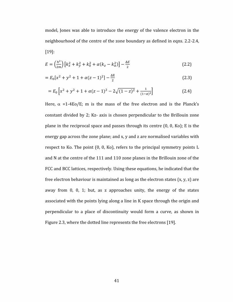
model, Jones was able to introduce the energy of the valence electron in the
neighbourhood of the centre of the zone boundary as defined in eqns. 2.2-2.4,
[19]:
(
) [
]
(2.2)
[ ]
(2.3)
[ √
] (2.4)
Here, =1-4Eo/E; m is the mass of the free electron and is the Planck’s
constant divided by 2; Kz- axis is chosen perpendicular to the Brillouin zone
plane in the reciprocal space and passes through its centre (0, 0, Ko); E is the
energy gap across the zone plane; and x, y and z are normalised variables with
respect to Ko. The point (0, 0, Ko), refers to the principal symmetry points L
and N at the centre of the 111 and 110 zone planes in the Brillouin zone of the
FCC and BCC lattices, respectively. Using these equations, he indicated that the
free electron behaviour is maintained as long as the electron states (x, y, z) are
away from 0, 0, 1; but, as z approaches unity, the energy of the states
associated with the points lying along a line in K space through the origin and
perpendicular to a place of discontinuity would form a curve, as shown in
Figure 2.3, where the dotted line represents the free electrons [19].

42
Jones essentially made a comparison of the valence band structural
energies between the face-centred cubic (FCC) and body-centred cubic (BCC)
Cu as a function of electron concentration (e/a) in the context of the rigid band
model, when he assumes that the addition of Zn to increase e/a does not
change the DOS of the parent Cu with the FCC and BCC structures, and the
parameter e/a can be obtained from eqn. 2.5 [19]:
(
) (
⁄
)√ (2.5)
Here, D (E) represents the DOS and Va is the volume per atom. A perfect
coincidence of the two parabolas over the energy range below about 5 eV for
the FCC and BCC-Cu indicate that Jones assumed,
in Eqn. 2.5. The
Figure 2.3: The energy of the states associated with the point lying along a line in K space through the origin, and perpendicular to a plane of discontinuity plotted against the distance from the origin. The dotted line represents energy of the free electron, after Jones (1934).

43
volumes per atom Va in FCC and BCC lattices are therefore obviously given by
respectively, where a is the lattice constant. The DOS equation
given by Jones therefore implicitly leads to the relation in eqn. 2.6. The energy
difference calculated by Jones from the density of states in Figure 2.4(a) is
displayed as Figure 2.4 b [20]:
(2.6)
The large kink found in the DOSs (see Figure 2.4(a)) represents the so-
called ‘van Hove singularity’, which Jones believed to be responsible for the
interpretation of the Hume-Rothery electron concentration rule [20]. To
account for the e/a dependent stability of the and β phases, Jones explained
that the van Hove singularity in the BCC Cu in Figure 2.4 was caused by the
contact of the Fermi surface with the 110 peak in the DOS of the BCC- Cu
(b)
(a)
Figure 2.4: (a) Density of states in the Jones model. After Jones (1937); (b) Energy difference calculated by Jones from the density of states in (a).

44
located about 1 eV higher than the 111 peak in the FCC-Cu e/a variation at
different Fermi surface. Jones’ work is displayed in Figure 2.5 [21].
Similarly, Jones tried to use the valence band structure energy U of the
respective phases to explain the /β phase transformation. He found U by
integrating the DOS multiplied by the energy E up to the energy corresponding
to the highest occupied states. The valence-band structure energy difference
between these two phases, U, is given as a function of e/a by eqn. 2.6:
⁄ ∫
∫
(2.6)
Here, the upper limit of the integral EFCC or EBCC is the energy for FCC or BCC
phases when the same number of electrons is filled into the respective DOSs.
By this relation, it follows that the relative stability of an alloy phase will be
enhanced if the DOS curve involves a large peak and a subsequent rapid
declining slope like in Figure 2.4(a), while the competing phase is fairly
Figure 2.5: The FsBz interaction in the Mott and Jones theory, A critical vale of (e/a) is obtained when spherical Fermi surface touches the zone plane of the respective Brillouin zone (a) the principal symmetry point L in the FCC Brillouin zone, (b) the principal symmetry point N in the BCC Brillouin zone, and (c) the symmetry point N330 and N411 in the Brillouin zone for the gamma-brass structure from Mott and Jones 1936.

45
monotonic for a given (e/a) range. It was not until 1957 that the error in Jones’
model was recognised, when Pippard [23] discovered the flaws and
inconsistency in the possession of neck in the Fermi surface contour of pure
Cu. It was only then that people became aware of the many unjustified
assumptions in the model, which had been made to conveniently account for
the Hume-Rothery rule. Although the early theories as proposed by Mott and
Jones in the 1930s were unfortunately far from being satisfactory, their work
provided an inspiration for interpreting the Hume-Rothery electron
concentration rule, which relates phase stability to the Fermi surface.
2.2.3 DV X and Md-parameter electronic calculation
The first theoretical approach to β-Ti alloys design was proposed
by Morinaga et al. [24] using the d-electron method based molecular orbital
calculation of electronic structures (called discrete variational X cluster
method, DV-X cluster method). Figure 2.6 shows changes in Md-Bo relation of
Ti by alloying. Two parameters were determined theoretically: namely, (i) the
bond order number (Bo), which is a measure of the covalent bond strength
between Ti and an alloying element; and (ii) the d-orbital energy level (Md),
which correlates the electronegativity and the metallic radius of the elements.
The values are defined for an alloy, the compositional average values of Bo and
Md parameters is defined according to the following eqns. [24]:
| | ∑ (2.7)
| | ∑ (2.8)

46
In their calculation, the two parameters, Bo and Md, are defined, where
Bo is related to the strength of the covalent bonding between Ti and an
alloying element, and Md is correlated with the electronegativity and metallic
radius of elements. According to the definition of the parameters, the average
value of Bo for alloys should be between 2.86-2.92 eV and the average value of
Md for alloys should be between 2.40-2.45 to attain low Young’s modulus.
Such a vector varies in direction and magnitude, depending on
elements, as shown in the vector map in Figure 2.6. The alloy position moves
in (Bo-Md) map as the alloy composition is altered. The areas for ; +β Ti
Figure 2.6: Bo-Md relations for various Ti binary alloys by Morinaga et al. [24] taken from Kuroda et al. [25].

47
based alloys are labelled as shown in Figure 2.7. (Positions of Ti and its alloys
are also shown in the Figure along with their Young’s moduli.) The stability of
elasticity of these alloys decreases with increasing Bo and Md and towards the
stability limit of the β phases; i.e., at the β/β + boundary for mainly Ti-Nb
alloy system.
Figure 2.7: [Bo-Md] map in which β/β + phase boundary is shown together with the boundaries for Ms=RT and For Mf=RT. The value of the Young's modulus (GPa) is given in parentheses for typical alloys.

48
2.2.4 First principle (DFT) electronic structure methods
There is still a large step from the theoretical considerations outlined
in the preceding section to a manageable form which can be run on a
computer. As the solution for a solid is desired, a natural condition is
translational symmetry for the observables, such as the potential,
eff (r + R) = eff (r): (2.9)
Here, R is a lattice translation vector. As a consequence of translational
symmetry, the wave function must fulfil Bloch's theorem [26],
(r + R) = eikR k(r) (2.10)
DFT is essentially based on the theorems of Hohenberg and Kohn [27],
who demonstrated that the total ground state energy E of a system of
interacting particles is completely determined by the electron density (). E
can therefore be expressed as a functional of the electron density and the
functional E[] that satisfies the variational principle. Kohn and Sham [28]
then rederived the rigorous functional equations in terms of a simplified wave
function concept, separating the contributions to the total energy as,
| | | | ∫
∫
| | (2.11)
The variational Kohn-Sham orbital may then be expressed as a linear
combination of basis functions obeying Bloch's theorem,
nk(r)=ci,nkik(r), (2.12)
with band index n and k representing a vector of the first Brillouin zone.
Building on energy functionals (i.e. the expectation value of the Hamiltonian)

49
and applying the variational principle, the solution to the Kohn-Sham
equations is transformed into a matrix eigenvalue problem,
∑ ⟨ | | ⟩ ⟨
| ⟩ (2.13)
This equation has to be diagonalised for obtaining the eigenvalues and
eigenvectors c from which the electron density is constructed and —
consequently — the total energy is derived.
Currently, the most widely used numerical methods for solving the
Kohn-Sham equations are: pseudopotential (and related) methods, the linear
muffin-tin orbitals method, the full-potential linearised augmented plane wave
method (FLAPW) [29], VASP and CASTEP codes [30, 31] using either
pseudopotential or the project augmented wave method, and a plane wave
basis set. In the present thesis, the commercial version of Cambridge Serial
Total Energy Package (CASTEP code) [31] is applied, which is one of the most
powerful ab initio DFT packages available at present. CASTEP is based on the
pseudopotential concept. For the actual calculations a generalised gradient
approximation (GGA) construction of the potential [32] is self consistently
applied, which is known to give very accurate results as tested by comparison
to FLAPW benchmarks. CASTEP has been already applied to a wide range of
problems and materials, to bulk systems, surfaces, interfaces, e.g. Refs. [32, 33,
34].
Other specific computational and technical aspects (e.g. number of k-
points, geometry of the unit cell etc.) are discussed later, together with the
results. The theory and parameters underlying the CASTEP code have been

50
addressed in the abovementioned publications. It should be noted that
CASTEP has also been applied to materials and systems which may be
considered 'well-established' from the computational point of view. The
CASTEP as implemented in the materials studio package served is a tool, which
works reliably when handled with care and knowledge. Convergency aspects
were carefully tested in several cases. Consequently, it can be argued that the
results as presented in following chapters do not depend on inherent technical
parameters and are physically meaningful.
2.3 Titanium metallurgy
Titanium metal is dominated by the allotropic transformation, but the
exact transformation temperature is strongly influenced by interstitial and
substitutional additions. A survey of the various phase transformations that
take place are presented in this section.
2.3.1 Classification of phase transformation
Titanium metal, both in its pure and alloyed states, undergoes a series
of allotropic phase transformations in equilibrium conditions from a high
temperature body-centred cubic crystal structure (BCC) phase with space
group of the form Im3m (No 229), to the closed-packed hexagonal crystal
structure (HCP) phase of the form P63Immc, (No.194), (see Figure 2.8) at
1155.5 K ( -transus temperature). The exact transus point is dependent on
the alloying composition and/or cooling rate regime [35, 36, 37, 38]. It can,

51
Figure 2.8: Schematic illustration of the unit cell of (a) HCP - phase with the three most densely packed lattice planes and lattice parameters at room temperature, (b) the BCC phase with one variant of the most densely packed [110] lattice planes, and the lattice parameter of pure at 1173 K.
however, be broadly classified as stable and metastable phases, depending on
the mode of achieving steady state conditions, where the thermodynamics of
phase stability is dominated by minimisation of Gibbs free energy (G)[39].
When higher heating/cooling rates are applied, non-equilibrium or metastable
phases possessing higher G are formed through displacive transformation by
shearing and shuffling mechanisms. In such circumstances, kinetics becomes
the dominant driving force behind choosing the exact mechanism for
transformation. The metastable phases might be temporal or permanent,
depending on the final processing condition.
In describing the phenomenon that favours the formation of
equilibrium phases, some metallic elements can be classified as being , or
neutral stabilisers [35]. The illustrations of these crystal structures are
presented in Figure 2.1(a) and 2.1(b).
(a) (b)

52
2.4 Titanium alloys and the phases
The substitutional elements — such as Al and the interstitial elements,
such as Al, B, Sc, Ga, La, Ce, Ge, O, N and C —extend the phase field and are
therefore referred to as stabilisers. Aluminium is the most common alloying
element to raise the transition temperature, while still having substantial
solubilities in both , and phases. Oxygen is occasionally considered an
alloying element, though only when it is used to obtain a desired property —
such as increasing strength in commercially pure titanium [36, 40]. The term
‘aluminium equivalent’ (Al. Eq.) is used to quantify the stability given by the
ratio of Al equivalent divided by the weighted averages of the aluminium
equivalent of the elements. The Al. Eq. is expressed as [36,37]:
(AlEq:) = Al +13Sn +16Zr + (O + C + 2N) per cent. (2.14)
Elements which are classified as stabilisers depress the phase field to
a lower phase transition field temperature [37, 38, 40, 41, 43]. They are
classified as either isomorphous or eutectoid elements. The -isomorphous
additions are mainly the BCC elements V, Mo, Hf, Ta, and Nb. They are usually
transition metals and noble metals in the periodic table which, similar to
titanium, have unfilled d-electron bands. Previous investigations have shown
that sufficient concentrations of these elements make it possible to stabilise
the phase at room temperature. Other isomorphous elements include Ta and
W, which are rarely used as alloying additions, because of density concerns.
Elements that have limited solubility range in phase and are able to

53
decompose via eutectoid reaction into plus a compounds are known as
eutectoid elements. The most commonly used eutectoid elements are Cr, Fe, W,
Pt, Pd and Si, Ni, Co, Au, Ag, Cu and Mn. The molybdenum equivalent defined as
Mo. Eq. 2.15 is used to express the stability (or stability) of a titanium alloy.
In equation 2.15, the different variables are associated with the ratio of
concentration for molybdenum divided by concentration for the particular
element. The parameter seems fairly accurate for binary alloys, but it is not
known how accurate it is in quantifying the stability in a heavily alloyed
multicomponent alloy. The Mo. Eq. is defined as:
[MoEq) = 1.0Mo + 0.67V + 0.28Nb + 0.22Ta + 1.5Cr + 2.9Fe + 1.0Al% (2.15)
Although it might be that no metallic element is purely neutral, some
elements are classified as neutral because they have a minor influence on the
transus temperature. They can lower the transus slightly, but again increase
it at a higher concentration. These elements include Sn, Zr and Hf, which may
slightly lower the / transformation temperatures after certain threshold
Figure 2.9: Schematic illustration of the relative effect of stabilising elements on a Ti alloy phase diagram after [35].

54
concentrations. Zr and Sn are the commonly used neutral stabilising elements.
Zr and Hf are isomorphous with titanium and therefore exhibit the same
allotropic phase transformation from to and are completely soluble in both
the and phases. Zr also substitutes titanium in a multicomponent alloy and
thereby indirectly has a stabilising effect [35-38]. Sn on the other hand
belongs to eutectoid elements and could have little or no effect on the /
phase transformation temperature. Sn is considered stabilising however, as
it replaces Al in the hexagonal ordered Ti3 Al. The relative effects of stabilising
elements on a Ti alloy phase diagram are schematically illustrated in Figure 2.9
after [35, 37, 38-43].
2.4.1 Equilibrium phases
Although the most common equilibrium phases are those of and ,
there are some intermetallic ordered phases that have been observed in
titanium alloys. A brief description of them follows.
(a) Hexagonal phase called apha martensite ():
Titanium in its pure form exists as a hexagonal closed packed (HCP)
structure at room temperature and pressure [38,40-43]. The HCP unit cell can
be defined by placing two atoms at (0, 0, 0) and (1/3, 2/3, 1/2) positions of its
unit cell, as shown in Figure 2.8(a), together with the three most densely
packed lattice planes and lattice parameters at room temperature. The phase
has a space group of P63mmc. The elastic moduli of single crystal of are

55
anisotropic in nature, varying between 145GPa (stress axis parallel to c-axis)
and 100GPa (stress axis perpendicular to c-axis); while the shear modulus G
ranges from 46GPa (stress applied in {1120} direction in (002) plane to 34GPa
(stress applied in (1120) direction in (1010) plane) [37]. As expected, this is
not the case in polycrystalline alpha. They appear as coarse grains while
cooled from phase region in nature; though a finer precipitate distribution in
a matrix can be observable in / after solution treatment with further
coarsing of the previously precipitated . The two scales of precipitations
formed at different stages of heat treatment process are referred to as primary
and secondary by metallurgists. In addition, within the matrix, another
cluster laths forms of belonging to one (colony) or multiple (basket weave)
crystallographic variants growing together are formed, depending on the
cooling or quenching rate evolving from the phase field. In general, the
morphology of this phase is dependent on factors such as parent morphology,
cooling rate, thermomechanical treatment and alloy content.
During deformation, several slip systems operate within the titanium
alloys system. The most common slip direction is 1120 . The direction slip
occurs in one (0002) basal plane, three {1020} prism planes, and six {1011}
pyramidal planes [38, 40-43]. They are therefore responsible for the four
independent slip systems. The fifth slip system required for homogeneous
deformation of polycrystals (Von-Mises criteria) is provided by the two basal
slips that occur in the 1123 direction and in the {1122} plane. If the slip
systems are unable to operate, twinning occurs in titanium. The main

56
twinning modes are {1012} and {1121} in tension and {1122} in
compression loading [37].
(b) Beta ()
This is normally the high temperature phase, when pure titanium is
heated above 1156K (known as the transus), allotropically transforms to
(BCC) structure, shown in Figure. 2.8. The BCC structure has two atoms per
unit cell and could be defined by placing the atoms at (0, 0, 0) and (1/2, 1/2,
1/2) positions. The space group is 1m3 m. As BCC is a more open structured
crystal, it can accommodate higher entropy required at elevated temperatures,
making BCC more stable at higher temperatures than HCP phase. The elastic
modulus E of phase measured at these temperatures is about 58GPa and the
shear modulus G is around 20GPa [36]. While the elastic constants — C11, C12
and C44 in phase — seem to be almost independent of temperature [39], pure
mono-crystals at 173 K have C11; C12 and C44 values to be 97.7 GPa, 82.7 GPa
and 37.5 GPa respectively [39]. As BCC is not a closed packed structure, the
deformation occurs by slip via different slip systems. The [110] planes have
the highest atomic density, but other planes — like [112] and [123] — come
very close. [111] direction is, however, a closed packed direction, thus there
are 48 slip systems operating in materials. As slip can occur in multiple
planes, the dislocation can readily cross-slip giving rise to wave slip bands
[37]. When slipping is hindered, twinning occurs in titanium alloys. The
different twin systems observed are {332},113 and {112} 111 [40].

57
(c) Beta2 called (β2)
This phase has two interpenetrating simple cubic sublattices; one
containing the corners of the BCC unit cell (0, 0, 0) and the other containing the
body centred (1/2, 1/2, 1/2) sites. Thus, 2 is actually a simple cubic structure
(space group Pm1 m superlattices). Evidence of this is common in several
binary and ternary titanium aluminates and Nickelides (shape memory alloy),
and is confirmed by the presence of {100} superlattice spots in a [001]
electron diffraction pattern. These spots are forbidden reactions according to
the BCC structure factor calculations which would not normally show up in an
ordinary disordered β2 structure. The nature of these {100} super reflections
— ranging from strong, weak or diffuse streaks — bears information about the
degree of ordering in a particular alloy. Quantitatively, the degree of ordering
is defined in the crystal via a long-range parameter L, such that L=1 for fully
ordered and L=0 is for completely random distribution [37, 43].
(d) 2 (alpha 2):
This is otherwise an ordered hexagonal solid solution of chemical
formula Ti3M (where M are simple metals such as Al, Ga, In or Sn), formed
instead of the disordered HCP phase. It has a DO19 structure with a unit cell
composed of four regular HCP cells seemingly supported by covalent-like
directional bonds connecting titanium and the simple metal atoms [37, 38].
This form is mainly due to the addition of higher concentration of alpha

58
stabilisers, as seen in the case of Ti3Al, 2 in alloys containing more than 6
Wt.% Al.
(e) (Gamma):
This is an intermetallic structure formed at still higher additions of
alpha stabilising elements. Predominantly, this phase occurs when about 50
at.% of Al has been added to titanium (TiAl). It has a L10 structure, with
alternating (001) planes of Ti and Al. It is known for being the cause of
increased embrittlement in Ti-Al alloys at 25 at.% Ti3 Al, 50 at.% TiAl and 70
at.% TiAl3 [38].
(f) O phase:
This is an ordered ternary Ti2AlNb phase that has been discovered in
the Ti-Al-Nb systems that may have potential for use as a structural material
for use at elevated temperatures [65]. This O phase has orthorhombic
symmetry (Cmcm) which occurs by Ti/Nb ordering of the hexagonal DO19
phase, or by Al/Al ordering of the cubic B2 phases. Alloys with microstructures
consisting of the O (i.e. /2 phases) have been shown to possess excellent
combinations of low and high temperature mechanical properties. Commonly
found in alloys consisting in atomic per cent ranging between 18-30% Al, 18-
34% Nb, and balance Ti.

59
(g) 82
This is another ternary phase in the Ti-Al-Nb system that was
discovered recently. This phase has a composition close to Ti4Al3Nb. It has
been described as being in apparent equilibrium with the, , Li0, 2, DO19 and
O (orthorhombic) phases [38-41], and it has been observed that it has the 82
structure of the omega phase. It forms readily at high temperatures from the
cubic B2 phase by the displacement of pairs of (111) and subsequent chemical
ordering.
2.4.2 Non-equilibrium phases (metastable)
As stated earlier, the phase(s) formed are dependent on a number of
conditions, including but not limited to the alloying composition and
processing treatment. Metastable (non-equilibrium) Ti phase(s) can be formed
due to varying alloy thermodynamic or kinetics, such as insufficient cooling
time for long range diffusion of atoms needed to arrange from one stable phase
to another ( to β and vice versa in the case of titanium). In general, the
phase(s) form as a compromise between thermodynamics that favour
minimisation of Gibbs free energy ΔG and kinetics which dictate how fast the
transformation can occur. The following sections offer a brief description of
some of the metastable phases encountered in titanium alloys.
(a) Alpha prime martensite
This martensitic phase forms instead of as a result of an extreme rate
of quenching in dilute titanium alloys from high temperature β phase. Its

60
crystal structure is hexagonal (P63mmc). In dilute alloys, the morphology
changes from colonies of lath to lenticular or a twinned structure, depending
on the solute contents [44]. In Ti-Mo alloys, it is said to have orientation
relationships between adjacent plates, consistent with the Burgers
relationship. This further indicates that the plates are formed by a martensitic
reaction. The microstructure is dominated by large plates of and β
precipitation (because both shear (martensitic) and diffusional growth
mechanisms are involved) [44].
Many metallic and non-metallic materials undergo a first order
transformation in the same fashion as in steel. For this reason, all other types
of lattice transformation (other than steel) without atomic diffusion are known
in physical metallurgy as a martensitic transformation [45]. In principle,
however, all metallic bodies can be made to undergo diffusionless
transformation, provided the cooling rate or stress rate is rapid enough to
prevent transformation by alternative means. Martensite is named after
eminent German metallurgist Adolf Martens, who was the first to observe the
structure of martensite in a quenched steel sample. The name ‘martensite’ had
been used mainly, and originally, to describe the structure formed in steel
quenched from a temperature of, say 960C, from face-centred austenite to
martensitic phase (-). The most familiar martensite formed in steel takes an
irregular shaped plate, which, in three dimensions, is a hard lens body centred
cubic described as acicular martensite [46]. Its formation is less likely as the β
stabilising elements increase in a titanium alloy because the martensite start

61
temperature decreases and thus the phase is less easily formed (as illustrated
in Figure 2.8).
(b) Orthorhombic martensite :
This is also formed by martensitic transformation, but with higher
solute concentration than [45, 46]. Its crystal structure is orthorhombic
(Cmcm) (no.63). The morphological structure is more or less an internal
twinned structure and, unlike , which can form by quenching only
(athermal), this can also form on application of external stress — hence the
name. Stress or strain induced martensite is formed as the name suggests,
upon the application of external stress or strain (see Figure 2,10).
Figure 2.10: Elastic deformation behaviour of Ti-24Nb-4Zr-7.9Sn alloy: the figure displays the stress–strain curves resulting from cyclic loading–unloading deformation with 1% strain step of the as hot-rolled alloy, thus demonstrating the recovery of incipient Young’s modulus after the work done by [76].

62
The detection of α" by x-ray diffraction (XRD) is relatively simple
because its characteristic pattern has five low angle lines compared to three
for α' [47]. A typical XRD pattern, showing reflections corresponding to the α"
phase, is shown in Figure 2.11 [48]. If the β phase was present in this Figure,
the first two reflections would occur at angles of ~38.5 (110β) and ~55.5
(200β).
Identifying α" by electron microscopy can be problematic, as other
crystal forms of the martensite phase have mistakenly been observed. For
example, a face centred cubic or tetragonal martensite has been detected in
some Ti alloys [47]. This was reported on the basis of thin foil electron
microscopy data. Evidence obtained by Williams [42], however, shows that
this martensite is orthorhombic in its bulk form. For example: when Ti-14V-
6Al is quenched from 900°C, XRD analysis of bulk samples shows that this
alloy contains α", whereas TEM examination of thin foils prepared from the
same sample shows evidence of a face-centred cubic martensite. Furthermore,
light microscopy of the thin edge of the electron microscopy specimens shows
marked rumpling, characteristic of shears resultant from mechanical
instability along the thin edge of the foil. In other alloys which observe α" in
bulk form, thin foil results show that α" reverts to the β phase along the thin
edge of the foil during thinning. Based on this evidence, Williams [42]
suggested that the reported face-centred cubic and/or face-centred tetragonal
martensites are in fact thin foil artefacts.

63
The microstructures of the and phase, however, have similar
acicular textures, characteristic of all martensitic phases. The difference is that
it is confined to higher compositional ranges. Considering that forms only at
higher amounts of alloying, it is therefore not surprising that the deformation
martensite is invariably of the orthorhombic variety, which is halfway between
the BCC β and the HCP Ti- phases [49]. This appears justifiable as HCP is just
a special type of orthorhombic structure with a/c =3; and for higher alloy
content when the constraints of hexagonal structure cannot be met, martensite
with orthorhombic structure are formed [50, 51] (see Figure 2.12).
Figure 2.11: XRD pattern of Ti-50Ta alloy after solution treatment at 950°C for one hour, followed by ice water quenching, showing reflections due to α", adapted from Zhou et al. [67].

64
It is surprising that the hardness of is much lower than and or
even β [52b]. This would have an influence on the elastic modulus. Though the
real reason behind it is not well known, one can guess that stretching of the
BCC lattice along two of its orthogonal pairs by contraction in the "c" axis and
expansion on the "a" and "b" axes leading to the formation of rectangular
prism such as that of ⦨ a, b and c are distinct. Thus changing the coordination
might play a part (see Figure 2.12).
The effect of some of these microstructural phases on the Young’s
modulus of binary Ti –Nb alloy is illustrated in Figure 2.13, after the work by
[53]. The Figure displays the correlation between Young’s modulus and e/a
ratio, which is similar for most Ti TM alloys. At low values of e/a, the β Ti
phase is unstable and the formation of the phase or martensite
Figure 2.12: A schematic illustration showing the lattice correspondence between the β and α" phases, taken from Kym et al. [52].
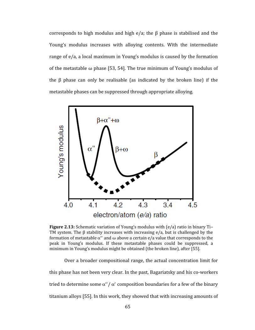
65
corresponds to high modulus and high e/a; the β phase is stabilised and the
Young’s modulus increases with alloying contents. With the intermediate
range of e/a, a local maximum in Young’s modulus is caused by the formation
of the metastable ω phase [53, 54]. The true minimum of Young’s modulus of
the β phase can only be realisable (as indicated by the broken line) if the
metastable phases can be suppressed through appropriate alloying.
Over a broader compositional range, the actual concentration limit for
this phase has not been very clear. In the past, Bagariatsky and his co-workers
tried to determine some / composition boundaries for a few of the binary
titanium alloys [55]. In this work, they showed that with increasing amounts of
Figure 2.13: Schematic variation of Young’s modulus with (e/a) ratio in binary Ti–TM system. The β stability increases with increasing e/a, but is challenged by the formation of metastable and ω above a certain e/a value that corresponds to the peak in Young’s modulus. If these metastable phases could be suppressed, a minimum in Young’s modulus might be obtained (the broken line), after [55].

66
Nb, Ti-Nb binary alloys undergo martensitic transformation upon quenching
from the high-temperature β- phase field to hexagonal or to orthorhombic
phases (these and martensites can be analogous to the high-pressure
and phases in pure iron respectively). The high temperature BCC structure of
titanium can be stabilised by alloying with TM elements to its right in the
periodic table. The border line between and has been linked to a certain
critical value of the e/a ratio discussed earlier. For many binary Ti-TM (TM =
metallic elements) alloys, the critical e/a ratio of 4.15 corresponds to
compositions that fall into the stability range of the martensite, with the
martensite start temperature (Ms) estimated to be 473 K [53, 55]. If the Ms
can be suppressed to below room temperature by further alloying additions,
the reversible β to transformation can be induced by applied stress at room
temperature. This idea formed the basis of continued efforts towards
developing shape memory and super-elastic titanium alloys of the β type [56,
57, 58, 59].
(c) Omega Phase (ω)
Perhaps the most studied among all metastable phases in titanium
metallurgy is ω. It is a submicroscopic precipitate that is supposed to be a
transition phase formed during the β to α transformation. Probably because
the complex morphology causes the most substantial change in the physical
and mechanical properties of the alloys (such as ductility and
superconductivity), the kinetics of its formation, as well as the nature of its

67
diffuse X-ray and neutron scattering, its mechanism of formation from the
parent β phase [60], and its formation are characterised by a series of special
features. The first reports of this phase were made in 1954 by Frost et al. [61],
who observed it in binary alloys of titanium with chromium and manganese.
Later, the ω phase was found in many other titanium alloys as well. The
compositional windows within which the ω phase will form, however, varies
according to the alloy system [62].
Over a broader composition range, the ω phase will occur as a
precipitation product of β decomposition during moderate temperature (300-
550°C) isothermal aging (ωiso). The formation of the ωath phase occurs by a
diffusionless, or compositionally invariant, transformation [42, 63]. This
transformation cannot be suppressed, no matter how rapid the quench rate
[49].
The detection of the ω phase, like the detection of α", can often be
difficult. In a recent study [64], the alloys Ti-30Nb-5Zr and Ti-30Nb-5Ta-5Zr
were both found to contain the ωath phase after solution heat treatment. The
presence of the ω phase, however, could mostly be precisely detected under
TEM, therefore suggesting that the particle size of the ω phase was very small.
When detectable by XRD, diffraction peaks of the ωath phase are typically broad
and of low intensity. In addition, because many of the ω peaks overlap with the
positions of the β peaks, typically only one or two singular ω peaks are
present. The ωiso phase is typically easier to identify with stronger reflections
in XRD. An example of an XRD pattern of a β+ωiso microstructure is shown in

68
Figure 2.14, for the recently developed biomedical alloy Ti-29Nb-13Ta-4.6Zr
[65].
It is well known that ω phase is related to the BCC parent phase
according to the <000l>ω||<111>β;{11 0}ω||{1 0}β orientation relationship,
implying the existence of four variants of the ω, with respect to the BCC lattice.
The ω lattice is obtained by collapse of neighbouring (111)β planes of a BCC
structure, leaving every third plane in place. The atomic movements required
are ± aβ √3/12, where aβ is the β lattice parameter or equivalently ± cω/6
where cω is the c axis of the ω phase. Complete plane collapse will produce the
ideal ω structure with aω = √2aβ and cω = √3/2aβ. For a partial collapse (<
aβ√3/12), the trigonal ω crystal structure is obtained [63]. Most ω crystal
detected by XRD is found to bear the hexagonal crystal structure.
Figure 2.14: X-ray diffraction pattern of Ti-29Nb-13Ta-4.6Zr alloy after solution treatment at 790°C for one hour, followed by water quenching, then aged for two days at 350oC, adapted from Li et al. [65].

69
Like the phase, it forms in all alloys of titanium with transition metals,
but only at a definite "critical" concentration of the alloying element. An
indirect proof of the two-stage occurrence of the process of ω phase
transformation in low alloys of titanium and in titanium itself is by volume
changes. By analogy with the volume effect in a β to ω transformation, one
should expect that the occurrence of the first stage of the β to transformation
should be accompanied by an increase in density (i.e. a decrease in volume),
and that the occurrence of the second stage (ω to ) should be associated with
a decrease in density. The understanding of the mechanism of omega
formation in titanium systems is mainly under these conditions [66].
(i) The ω phase is the product of transformation of the metastable
β solid solution. Experimental evidence suggests that the process of the β to ω
transformation never reaches completion; i.e. the disappearance of the
complete β solid solution — the ω phase always coexists with the metastable β
phase.
(ii) The lattice constants of the ω phase are practically
independent of the conditions of formation (hardening or tempering) and of
the type of alloying elements.
(iii) The process of β to ω transformation on hardening alloys from
the "critical" concentration takes place at approximately the same or
neighbouring martensite temperatures Ms, which are relatively low (573-
890K), independently of the alloying elements. This can be distinguished from
the athermal by its large size and a composition gradient along ω /β interface.

70
(iv) The temperature of formation of the ω phase during the
tempering of more highly alloyed metastable solid solutions is approximately
180–500°C, which is practically equal to the temperature of formation of the ω
phase during hardening (Ms).
(v) The formation of the ω phase is always accompanied by an
increase in the density of the alloys.
(vi) As was noted above, a characteristic feature of the ω phase is
that it does not show up under the optical microscope and the difficulties arise
in the interpretation of its crystal structure.
(vii) Its deformation at room temperature and application of higher
pressure has also shown to stabilise ω phase under certain circumstances.
Studies on Ti-Cr and on Ti-V alloys by Bagariatski et al. [54b] have shown an
increase in ω phase on deformation.
In a similar move with , a link was made by Luke et al. [54a]
concerning the occurrences and stability of ω phase and e/a ratio of 4.06-
4.14eV for ω-Ti phase formation from experimental data. This was disputed by
authors such as Hickman, however, who noted that the stability of the ω phase
in alloys could not be predicted from the e/a ratio alone [67]. The position of
alloying element in the periodic table is also an important factor; this is
thought to be because of the d-band and s-d band hybridisation influence on
the electron density of state.
Blackburn and Williams tried to gain an insight into the composition of
the ω phases, estimating its volume faction in Ti-Mo alloys by electron

71
microscopy [68]. Their findings seem to be in an agreement with the work of
Silcock et al. [69] on the structure of ω phase in titanium alloys. They both
agreed that the structure was hexagonal with a=4.60Å A and c=2.82 Å (c/a=
0.613). They differed, however, on the type of structure they found: while
Silcock et al. believed the atomic position to be (0,0,0) and (2/3, 1/3, 1/2)
belonging to P6mmm space group as HCP, Bagariatski and co. [70] thought it
to be at (0, 0, 0) and (2/3, 1/3, ), where is equal to 0.48 0.01Å — therefore
possessing P3 ml space group, which is a trigonal structure instead.
In reality they are both correct, as it can be either hexagonal or trigonal
depending on whether the transformation is complete or in the initial stages
[62]. This was later clarified by Sass, who observed that ω SAD patterns have
straight or curvilinear lines of diffuse intensity instead of sharp spot [71]. The
latter, referred to as the “diffuse ω phase", relates to the early stages of ω
formation.
As a result, Blackburn and Williams devoted a lot of effort to their
groundbreaking work relating to the ω phase morphology with misfit strains.
Here, the authors studied Ti-Mo and Ti-V alloys at various stages of aging and
found a similar ellipsoidal morphology of ω with a major to minor axis ratio of
about 2.2. In Ti-V alloy however, the ω precipitates were approximately cube-
shaped with sides of the cube parallel to (2021) ω [72, 73]. They observed
that, for all Ti-(3d) transition metal alloys with unfilled 3d electronic shells
(like Ti-V, Ti-Cr, Ti-Mn and Ti-Fe), the ω phase is cubic-shaped when visualised
on the TEM microscope; whereas for Ti-(4d)Tm alloys (i.e. transition metals

72
with unfilled 4d electronic shells — like Ti-Nb and Ti-Mo), the ω phase is
ellipsoidal in shape [74, 75]. They inferred that the precipitation morphology
is related to the Ti/transition Metal atomic volume ratios or their lattice
misfits. In Ti-Nb and Ti-Mo alloy systems, the misfit was small and the
ellipsoidal particle shape seemed dominated by the minimisation of the
anisotropic surface energy. In Ti-V, Ti-Mn, Ti-Fe and Ti-Cr systems, the misfit
was greater and the precipitate morphology cubic-shaped and determined by
minimisation of the matrix elastic strains. A value of 0.5% misfit was quoted,
below which the precipitate would be ellipsoidal in nature, and above which
would yield cubic ω morphology [74, 75].
(d) β: we commented earlier on how increasing the beta alloying additions to
pure titanium martensitic and omega phases formed on quenching. At still
higher β stabilising alloying additions, however, (i.e. the solute rich β Ti alloys
undergo a phase separation reaction to form β1 and β2. This could occur
either by classical nucleation and growth or a less observed spinodal reaction.
A number of criteria determine which of these two mechanisms would be
predominant. From a pure kinetic aspect, for spinodal reaction to occur the
quenching rate should be optimal: neither too fast to prevent short-range
diffusion of atoms, nor too slow to form the equilibrium β and phases. It is
important to note that β1 and β2 are just a convention referring to the two
phases as having the same crystal structure as the parent β phase (BCC), but
with different solute content and lattice parameters. Conventionally, β1 is
assumed to be the solute lean phase and β2 the solute rich phase. Sometimes,

73
in the literature, the β1 is referred to as β and β2 as simple β [42]. This β
usually remains as coherent and distributed in the β isomorph matrix. The
above description may not be exhaustive in terms of some of the equilibrium
and non-equilibrium phases observed in titanium alloys; but the most
important ones, and the influence of alloy properties that are useful for
engineering applications, have been mentioned. The following section will
explain some aspects of martensitic transformation from the high temperature
β phase that is peculiar to some of our main work on beta isomorphs Ti alloys
(Ti-Nb and Ti-Mo).
2.5 Some aspects of transformations in βTi – (Mo, Nb)
alloys
As discussed earlier, phase transformation occurs whenever a materials
system is not at equilibrium, or changes its microstate, as a result of external
constraints such as pressure or temperature. In effect, these materials adopt
different crystal structures favourable for the minimisation of their free
energy. In general, the microstructural features and the order in the system
changes, leading to variations in most of the important properties. By so doing,
phase transformation provides an effective way to modify the microstructure
of solids. If it can be activated by a mechanical or other physical force, it
becomes part of the deformation process and directly affects the properties of
materials as well [76].

74
There is possibly satisfaction to be derived from possessing an
understanding of phenomena such as martensitic transformation in metals
and alloys. The present work, however, deals with the basic mechanisms of
phase stabilities, therefore providing insight into the mechanical and chemical
properties of materials which are necessary for the design of new materials. In
this section, some of the structural, crystallographic and morphological
characteristic changes that take place as a result of phase transformations in
titanium alloys are briefly described.
Figure 2.15: Schematic illustration of the distorted closed-packed hexagonal cell (HCP), as derived from the parent BCC lattice after Burgers [82].

75
2.5.1 Shear transformations of β to (/)
As explained earlier, a martensitic transformation involves
homogeneous movement of atoms. Ideally, such a process is not involve
thermally activated and takes place at an extraordinary speed [45]; but in
practice a clear cut separation of transformation process into nucleation and
growth and martensite is generally not possible [77]. Based on such a premise,
we assume that diffusion does not occur and atomic correspondence is
maintained during such transformation. Independent theories to this effect
have been put forward by others [78]. Although in pure titanium metal a
simple athermal martensitic transformation is conceivable, in an alloy the
situation is more complicated for the following reasons.
The long-range effect of alloying, described, for example, in terms of
changes to the elastic parameter, may simply be to change the conditions
under which athermal transformation takes place. The local effect of alloying,
on the other hand, is to inhibit the movement of atomic, and thereby, (1)
reduce the distance over which atomic regions can cooperate, thus perturbing
the microstructure of the transformation product; and (2) reduce the speed of
the transformation, thus bringing it into completion with nucleation and
growth mechanisms [62]. This could inhibit the necessary microstructure of
the transformed product and rate at which such a reaction takes place [62].
The diffusion coefficient of the solute species in Ti was also thought to play a
large role in the evolution of crystallographic texture and during phase
transformations, which has a direct effect on the internal microstructure and

76
properties of retained phases of the alloy while quenching. For example: the
work of Jepson et al. [79] on the kinetics of transformation in Ti-Nb alloys
found the critical cooling rate at which martensite always formed (equivalent
to reaching the Ms temperature in terms of the TTT diagram of the alloy)
decreasing with increasing Nb content [80]. From these findings, the influence
of alloy content on crystallographic orientation in different Ti based systems
was made very apparent. Previous investigations [76, 80] have shown that
such a cubic β to hexagonal transformation occurs via a habit plane near
{334}β. One of these two different martensites would be formed, and β to
transformation process would be reducible to the activation of following shear
systems that follow a well-established Burgers relation [81]: i.e. (110) ∥
(0001); [111]β∥ [110] (see Figure 2.15). A study of the orientation
relationship in zirconium Burgers [82] proposed that the martensite
transformation of body centred cubic (BCC) to close-packed hexagonal (HCP)
occurs by a heterogeneous shear on the system BCC [ ] . This
distortion is illustrated in Figure 2.15. The crystallographic principle
underlying this proposal is that the configuration of atoms in the (112) plane
of a body-centred cubic structure is exactly the same as that in the (1010)
plane of a close-packed hexagonal structure based on the same atom radius.
The pattern on both of these planes is a rectangle √
√ ⁄ , where d is the
atom diameter. Thus a hexagonal close-packed structure can be built up from a
body-centred cubic structure by displacing the (112) planes relative to each
other. It should be noted, however, that the array on the (110)β planes (see

77
Figure 2.15) cannot be converted into an exact hexagonal array merely by the
pure shear proposed by Burgers, since the spacings of the (ll2)β planes and
[ ] planes into which they transform are not equal. Nevertheless, this
mechanism leads to approximately the observed orientation relationship.
Accordingly, the orientation relationship between the β and the (/) were
found to be same as the burger orientation relationship between the β to
type [49, 60, 83, 84]. This was schematically illustrated in Figure 2.16, after
[84], the basal plane of is derived from the [011]β-type plane and those of
[011]β and [100]β directions transform into [ ] and [ ] directions,
respectively. The closed packed direction [ ] and [ ] lying on the
{ } plane transformed to closed packed ⟨ ⟩ directions. The other
⟨ ⟩ directions are derived from ⟨ ⟩ directions. Based on this orientation
relationship and the symmetries of the cubic and hexagonal structures, a total
of 12 crystallographically distinct variants of the alpha phase can result from
the transformation of a single beta grain. It is not surprising that, to maintain
such orientation, a relationship has to be achieved via a series of contraction
and expansion of the β lattice in order to form (/). This is listed, according
to [78], here:
a 10 % contraction of [ ] corresponds to ⟨ ⟩
a 10% expansion along [ ] correspond to ⟨ ⟩
a 1% contraction [ ] corresponds to ⟨ ⟩
The orthorhombic crystal structure can be described as a slightly distorted
hexagon with the same atomic positions as in hexagonal, but distorted so

78
that the lattice parameter is in between the phase and β phase. It is said to
form by a degeneration of the hexagonal structure in form of a compromise
between the two. This is better illustrated when the Burgers orientation is
written in terms of the orientation crystal lattice. Hatt et al. deduced that, in
quenched Ti-Nb alloy, the following crystallographic adjustments have to be
made to get the observed orientation relationship [85]:
[ ] is 2° from ⟨ ⟩
[ ] is 2° from ⟨ ⟩
[ ] is 2° from ⟨ ⟩
This orientation relationship outlined above and in Figure 2.16 shows
the interrelationship between the three lattices as represented in the
orthorhombic system [63]. It is no surprise that as more and more β stabilisers
are added, the orthorhombic parameters change and become closer to the BCC
dimensions [84, 85, 86]. In the past, several quenched binary titanium alloys
(including Al, Mo, Nb, V, Au and Ag) were investigated for the presence of
martensites. Apart from Ti-Al, alloys were β to was impossible to suppress
[80]; all the other alloy additions are β formers, though — by definition — they
do not promote martensitic formation. The size and the cooling rate of the
specimen were, however, quite rigid and a bit confusing to understand. As a
consequence, even when thin slices of these alloys typically would not form
martensite, thicker ones would do due to the thermal shock experienced while
quenching.

79
Also, in lean Ti-Mo alloys, Davis and co-workers did find martensite on
quenched and un-quenched conditions [86]. They observed that with the
increase in Mo concentration, the structure changed from to and then to
completely retained β. So, at less than 4wt. %, formed; and above it, there
was the presence of martensite. It was indicated that, at low Mo
concentrations, the critical cooling rate for 1005°C/min transformation to
was not achieved on water quenching and thus there was a competition
between shear and diffusional transformations. At a higher Mo content (> 4wt.
%), the martensite start temperature, Ms and the critical cooling rate
decreased and thus a complete shear transformation occurred [87]. This was
similar to what Ho et al. [88] observed with 6-20 wt. % Mo titanium alloys. At
7.5 wt. % Mo, phase was seen to form with the lowest hardness; but at
about 10-12.5 wt.% Mo, the alloys showed increased hardness values due to
retained β.

80
In the Ti-Nb systems, these effects have been studied by several other
groups [88]. It has been found that at < 13wt. % Nb, was formed while
higher concentration yielded [89]. The evolution of and in some Ti-Nb
and Ti-V alloys were studied by some others including [90]. Similar
investigations on titanium based on eutectoid systems (Hypoeutectoids, such
as T-Ag and Ti-Si, and hypereutectoids, such as Ti-Au) by Menon et al.
confirmed the identification of massive β to m transformation [91, 92].
Stress-induced α" martensite (SIM) can be triggered in quenched
metastable β alloys by application of an external stress [93]. The triggering
Figure 2.16: Atom movements postulated by Burgers for the body-centred cubic to close packed hexagonal transformation in zirconium. On the left are body-centred cubic cells, and in heavy lines a cell having as a base and as vertical
sides, the latter serving as shear planes when the two hexagonal cells at the lower right are produced.

81
stress (σSIM) inducing the formation of α" rises with an increase in the stability
of the metastable β phase. Some alloy compositions, e.g. Ti-24Nb-4Zr-7.9Sn
[94, 95] (wt. %) exhibit both types of martensitic transformation; i.e. α" can be
induced athermally or by the application of an external stress [62]. The
thermoelastic reversibility of SIM is responsible for the observed shape
memory effect and superelasticity in some β Ti alloys. Athermally, evidence of
stress induced martensite transformation in deformed samples is revealed
through the cusp (kinks) present in their tensile stress strain curves. The
sudden jump in strain occurs usually to accommodate the β to
transformation and from lattice invariant during deformation. The physical
basis for transformation to the to occur in Ti–Nb and Ti-Mo based alloys is
that Nb or Mo stabilises the BCC structure with respect to HCP titanium, but
destabilises it with respect to the martensite by reducing its elastic shear
modulus. The composition of our alloy corresponds to small elastic shear
modulus [38, 54], ⁄ and, as such, {110} shear or shear along
[111] on {110}, {112} or {123} will be particularly easy [121]. It was
demonstrated that one of the three most probable mechanisms of the
transformation to the in BCC titanium is accomplished partially [110] {110}
atomic shuffles in opposite directions on every other {110} plane. The highly
anisotropic slip may also produce defect configurations such as kink bands
[53].
For high β content alloys too rich to undergo such transformations,
deformation while undergoing tensile stress can be attributable to mechanical

82
twinning. TEM images in Figure 2.17 reveal further details of the substructure
associated with this transformation and the variation of martensite
microstructure, including internal twins in Ti (20, 22, and 24) Nb alloys shown
in Figure 2.17 [97].
Several deformation mechanisms have been studied in Ti-based alloys
systems. It appears that the concentration and type of solute strongly
influences whether the stress-induced product in a given alloy is twinning or
α" [49]. In some alloys, clear evidence of mechanical twinning has been
observed, while evidence of α" has been obtained in others, or both. Due to the
Figure 2.17: (a), (b) and (c) are TEM images showing the variation of martensite microstructure including internal twins in the Ti (20, 22, and 24) Nb alloys. (d) is [111] β SAD pattern and the index that were obtained from the circle in (b), and indicating that the internal twins are of Type 1 twinning on (111) β plane after [4]

83
difficulty involved in discerning between deformation products, it has been
suggested that light microscopy is insufficient to identify the product since
both the twin and martensite have a similar appearance (as shown in Figure
2.18). The existence of twinning in the microstructure points have been
studied in Ti-Mo [98], T-V [99], Ti-Mn [100], Beta III [101] and Ti-15V-3Sn-
3Cr-3Al [102] alloys. These alloys have shown to exhibit two twin systems:
{332} [113] and {112} [113]. Both the {334} and the {344} martensite are
found in Ti-Mo alloy systems, a transition occurring between 10.5 and 11.5%
Mo. The {344} martensite found in the higher Mo alloys are usually formed by
deformation of the quenched alloy [98]. It has been suggested, however, that
light microscopy is insufficient to identify the product since both the twin and
martensite have similar appearance (as shown in Figure 2.18). XRD patterns
obtained from the samples in Figure 2.17(a) show no additional peaks, other
than those from the β phase, indicating that the lenticular features in the figure
are BCC twins. Electron microscopy has verified the formation of {112}<111>
[49] and {332}<111> twinning during stressing of Beta III and many other
metastable β alloys. The stress-induced product in Ti-14Mo-3Al in Figure
2.18(b) was identified as α". The evidence therefore suggests that high
resolution XRD is the most reliable way to detect the crystal structure of the
martensite phase [103].

84
2.5.2 The similarities between ω and transformation
Some close uniformity could be drawn between the shearing and
shuffling transformations of β that could lead to respective formation of ω and
. Some work has been done on compositional ranges and quench rates
applicable for the formation of each of these phases. Mofiat et al. [90]
investigated the Ti-Nb alloy system having between 20-70 atomic % Nb to
understand the competition between ω and . They established that and
ω precipitation specifically in Ti-Nb systems was favoured by fast and slow
quenching rates respectively, which confirmed the belief that, at slower
quench rate, the collapse of the (111)β planes are more complete. This was
similar to the result presented by Ohmori et al. [103], which showed that in Ti
alloys with the progress of ω phase precipitation, the β to transformation
was quite largely suppressed.
In order to determine the underlying similarities between these
metastable phases, the theory of localised soft phonon mode of transformation
was introduced by de Fontaine [104, 105]. Cook [106, 107], Clapp et al. [109]
Figure 2.18; Light micrographs of lenticular stress-induced products in: (a) Ti-11.5Mo-4.5Sn-6Zr (Beta III), and (b) Ti-14Mo-3Al, taken from Williams [49].

85
and Suzuki [110] compared martensitic transformation to spinodal
decomposition, which in itself is related to the ω phase precipitation. It is well
understood that while the spinodal reaction takes place through compositional
fluctuations, the ω grows by displacement fluctuations. Similar to the spinodal
mechanism, the martensitic transformation could therefore be triggered by
strain fluctuations in the vicinity of a strain spinodal. In addition, from the
neutron diffraction studies of Moss et al. [111] and the Mossbauer-effect
measurements of Batterman et al. [112], it can be said that the ω also
possesses strain fluctuations. This further narrows down the difference
between martensite and ω, and one can safely say that they are manifestations
of the same β instability phenomenon.
2.6 Evolution of β Ti alloy for orthopaedic implant
During the first part of the arthroplastic surgery development,
stainless steel was considered as a one of the viable implant materials, mainly
because of its availability and processing ease. Alloying additions of chromium
(Cr), nickel (Ni) and molybdenum (Mo) were made to the ferrous (Fe) matrix
to prepare alloys like 316L, also known as ASTM F-138 [113]. They were
primarily used to make temporary devices such as fracture plates, screws and
hip nails; but gradually, as TJR (total joint replacement) surgery became
popular, it became evident that very high modulus of stainless steel
(~200GPa) (Table 2.1) would be a deterrent. Researchers also started looking
for alloys that were more biocompatible and corrosion and wear resistant.

86
Cobalt (Co) based alloys came into the picture, while wrought alloys were used
to fabricate prosthetic stems and load bearing components. Even though they
offered excellent corrosion resistance, wear resistance and fatigue strength,
these Co-Cr-Mo alloys (ASTM F-75, ASTM F-799) still had higher modulus
(~210GPa) [see Table 2.1] and inferior biocompatibility to that desired for
implant materials [113]. As a consequence, after the early 1970s titanium
alloys started to gain popularity due to their excellent specific strength, lower
modulus, superior tissue compatibility and higher resistance [114].
The commercially pure titanium (ASTM F-67) was the first trial due to
the fact that its oxide (titanium in the atmosphere readily forms an oxide
coating around it) had excellent osseo-integration properties — i.e. human
bone cells bonded and grew on the titanium-oxide layer quite effectively. Due
to its limited strength however, the implants were confined to specific parts,
such as hip cup shells, dental crown and bridges, endosseous dental implants,
pacemaker cases and heart valve cage [115]. In order to improve the strength
for load bearing applications — such as total joint replacements — the alloy
Ti-6Al-4V ELI (ASTM F-136; the Extra Low Interstitial alloy composed of
Titanium (Ti), 6 wt. % Aluminium (Al) and 4 wt. Vanadium (V) and Ti-6Al-4V),
which was originally developed for the aviation industry. The elastic modulus
of about 110GPa (See Table 2.1), which was about half of 316L stainless steel
was chosen. As this was used for TJR surgery with modular femoral heads and
long term devices like pacemakers, it was soon found out that the presence of
vanadium caused cytotoxicity and adverse tissue reactions [202, 203]. Thus

87
niobium (Nb) and iron (Fe) were introduced, replacing vanadium, to develop
alloys such as Ti-6Al-7Nb [116] and Ti-5Al-2.5Fe [117]. Also other alloys with
aluminium additions like Ti-15Mo-5Zr-3Al [118] and Ti-15Mo-2.8Nb-3Al [113]
were tried out. Further studies, however, showed that the release of both V
and Al ions from the alloys might cause long-term health problems, such as
peripheral neuropathy, osteomalacia, and Alzheimer’s [119,120].
Consequently, Ti-6Al-4V somewhat lost its importance as the most viable
orthopaedic alloy.
Due to demographic changes and a worldwide increase in the average
age of the older population, which has led to a rapidly increasing number of
surgical procedures involving prosthesis implantation, there was an urgent
need to develop newer and better orthopaedic metallic alloys. For this, the
researchers first had to identify the metallic elements that were completely
biocompatible as to alloy with titanium. The ideal recipe for an element to be
used for implant application was excellent biocompatibility with no adverse
Alloy Modulus(GPa) Yield Strength (MPa) UTS
Stainless steel 200 170 465-950
Co-Cr-Mo 200-230 275-1585 600-1795
c.p. Ti 105 692 785
Ti-6Al-4Al 110 850-900 960-970
Table 2.1:Comparison of mechanical properties of commonly-used orthopaedic alloys.

88
tissue reactions effect, excellent corrosion resistance in bodily fluids, high
mechanical strength and fatigue resistance, low elastic modulus, low density
and good wear resistance. Regrettably, only a handful of elements will not
cause harmful reactions when planted inside the human body [121]: titanium
(Ti), molybdenum (Mo), niobium (Nb), tantalum (Ta), zirconium (Zr), iron (Fe)
and tin (Sn). Out of these, only tantalum showed an osseo-compatibility similar
to that of titanium; but its high atomic weight hindered it from being used as a
primary alloying addition. In fact, biocompatibility of higher amounts of
tantalum and palladium additions was only tested for dental and craniofacial
prosthesis where implant weight would not be of much concern [122]. For
other types of load bearing implants, several molybdenum and niobium based
alloys were analysed. For example: investigations on ternary Ti-Mo-Fe alloys
were carried out where the strengthening effect of Fe addition was studied in a
Ti-7.5Mo alloy [123, 124]. Another time, Guillermot et al. conducted tests on
Ti-Mo-Fe-Ta alloys with hafnium (Hf) additions [125]. Previous work by
Feeney et al. considered one of the most promising quaternary molybdenum-
based β-Ti alloys, Ti-11.5Mo-6Zr-4.5Sn, also known as βIII [126]. The phase
transformations occurring in these alloys were found to be similar to those of
binary Ti-Mo alloys. At room temperature the as quenched βIII alloy showed
low yield strength, high ductility and high toughness. The effects of iron on Ti-
Mo alloys [123] and the superior properties of βIII [126] were finally
combined to develop Ti-12Mo-6Zr-2Fe [127, 128], which recorded superior
yield strength and modulus values. As discussed earlier, it was believed that

89
the ω phase precipitation had a great effect on the strength of these alloys. A
parallel if not better effort was put in to develop niobium based β-Ti alloys.
Karudo et al. [25] and Tang et al. [129] developed alloys based on the Ti-Nb-
Ta, Ti-Nb-Ta-Zr, Ti-Nb-Ta-Mo and Ti-Nb-Ta-Sn systems. Of all the different
alloys that were chosen, the tensile strength and elongation of Ti-29Nb-13Ta-
4.6Zr alloy was found to be greater than, or equivalent to, those of
conventional titanium alloys for implant materials [130, 133]. Upon comparing
the hardness values of the quaternary alloys, it became evident that the
homogenised samples had higher hardness than the air or water quenched
samples. Finally the dynamic moduli was observed to be lowest at 5 at% Zr
and Nb/Ta ratio of 12.0, which was attributed to the preferred site occupancy
of Nb, Ta and Zr within the BCC unit cell and its effect on the nature of bonding
[130]. The alloys that possessed the lowest moduli were Ti-35.5Nb-5.0Ta-
6.9Zr and Ti-35.3Nb-5.7Ta-7.3Zr.
Consequently, based on this research, a number of contemporary and
prospective alloys were developed. These included Ti-12Mo-6Zr-2Fe [127,
128] and Ti-15Mo-3Nb-0.3O [134]. Additional inclusion of Interstitial Oxygen
(O) in the alloy, also referred as TIMETAL 21 SRX, Ti-13Nb-123Zr [135], Ti-
25Nb-4Zr-7.9Sn [93] and Ti-35Nb-7Zr-5Ta [136]. Happily, all these alloys
were primarily β or β+ type Ti alloys. The change in the direction of the
search for better biomaterials from /β Ti to β and β+ could be explained
by the fact that the latter fitted in very well with the tight mechanical
properties requirements of orthopaedic alloys. The standard requirement on
90
which such important properties decisions on modern day implants can be
based will now be discussed.
(a) Yield strength: The yield strength would determine the load bearing
capability of the implant. For TJR (total joint replacement) surgeries, where
load-bearing capability is indispensable, ideally a high strength value of the
alloy would be desirable. Hence, an alloy intended for orthopaedic use should
combine a high strength value with adequate ductility (defined by percentage
elongation or percentage reduction of area in a standard tensile test). Table 2.2
below lists the yield strength and ultimate tensile strength values of some of
the common titanium alloys. One would see that some of the metastable β
titanium alloys do show very high values in comparison to the or /β
titanium alloys.
(b) Elastic Modulus: A number of experimental techniques have been
used to determine the elastic properties of solids [137]. The relative elastic
modulus of implant compared to that of the bone (10-40 GPA) has always
been a source of concern [113]. Long-term experiences indicate insufficient
load transfer from artificial implant to the adjacent remodelling bone may
result in bone re-absorption and eventual premature loosening of the
prosthetic device [138, 139] due to the complex nature of compressive and
tensile activities which they are exposed to when the implant is in service. This
is termed the “stress shielding” effect, caused by the differences in flexibility
and stiffness, dependent partly on elastic moduli difference between the
natural bone and artificial implant material [140]. A reduction in the stiffness

91
of the implant by using a lower modulus material would therefore definitely
enhance the stress re-distribution of the adjacent bone tissue, ultimately
minimise the stress shielding effect, and eventually prolong the service life of
the implant device. In these terms, Ti6Al-4V and related /β alloys have been
considered to be inferior. The metastable β .e. m crostructure predom nantly
consisting of +β phase) and some fully transformed β phase exhibit lower
overall moduli. Figure 2.13 shows the interrelationship of elastic moduli with
microstructure; and Table 2.2 shows that Ti-15Mo-5Zr-3Al, Ti-12Mo-6Zr-2Fe,
Ti-15Mo-2Nb-0.3O and Ti-13Nb-13Zr have an elastic moduli ranging from 74-
88GPa, which is about 2-7 times higher than the modulus of bones.
There have been numerous previous attempts (some failed and some
successful) and many more will probably be developed and tested in the near
future. The Ti-33Nb-7Zr-5Ta and Ti-24Nb-4Zr-7.9Sn alloys, however, stand
out as prospective alloys mainly because they had one of the lowest modulus
to date (55 GPa and 24 GPA respectively): almost 20-40% lower than those of
other available alloys [106, 136, 93]. Ti-24Nb-4Zr-7.9Sn was developed by Hao
et al. of Shenyang National Laboratory for Materials Science, Institute of Metal
Research, Chinese Academy of Sciences, in China; while Ti-33Nb-7Zr-5Ta was
developed by Dr. Henry Rack at Clemson University and is now commercially
sold by Allvac ® as TiOsteum® and TiOstalloy®, and its low yield strength
value (547 MPa) was increased by adding interstitial oxygen. Thus Ti-33Nb-
7Zr-5Ta-0.4O showed the strength of 976 MPa and elastic modulus of 66GPa
[136]. It has been suggested that a two-step aging (instead of one) — one at a

92
low temperature and a second at a high temperature — could be a means of
increasing the yield strength. This is because the first step might lead to
nucleation of fine distribution of ω as a precursor for nucleation, which
would be coarsened to a desired strength in a relatively higher temperature at
the second aging step [141, 142].
Alloys designations Microstructure E(GPa) YS(MPa) UTS(MPa)
c.p Ti {} 105 692 785
Ti-6Al-4V {/β} 110 850-900 960-970
Ti-6Al-7Nb {/β} 105 921 1024
Ti-5Al-2.5Fe {/β} 110 914 1033
Ti-12Mo-6Zr-2Fe {Metastable β} 74-85 1000-1060 1060-1100
Ti-15Mo-5Zr-3Al {Metastableβ}
{aged +β}
75
88-113
870-968
1087-1284
882-975
1099-1312
Ti-15Mo-2.8Nb-3Al {Metastableβ}
{aged +β}
82
100
771-1215 812
1310
Ti-13Nb—13Zr {/β} 79 900 1030
Ti-15Mo-3Nb-0.3O (21Srx) {Metastableβ}+
Silicides
82 1020 1020
Ti-35Nb-7Zr-5Ta {Metastable β} 55 530 590
Ti-35Nb-7Zr-5Ta-0.04O {Metastable β} 66 976 1010
Ti-24Nb-4Zr-7.9Sn {/β} 24 900 920
Table 2.2: Orthopaedic alloys developed and/or utilised as orthopaedic implants and their mechanical properties (E=Elastic Modulus, YS=Yield Strength, UTS-ultimate Tensile Strength [113, 93].

93
2.7 Summarising comments
In summary, one must appreciate the growing interest in Ti and its
alloys and its ability to possess a range of property values depending on
alloying additions and/or thermomechanical treatments adopted. Though
significant advances have been made by alloying or micro-alloying as an
effective means of improving those properties and exploiting their potential as
materials for load-bearing components, these efforts are unfortunately still far
from the final goal in terms of understanding the microstructural
development, preventing poor ductility and toughness at ambient
temperature. This work attempts to identify the effect alloying additions have
on the mechanical behaviour and thermodynamic stability of and β Ti
phase and its dependence on initial β matrix instabilities. Chapters 3 to 7
discuss this approach and the results, which are then summed up in Chapter 8.

94
2.8 References
[1] Hume-Rothery W.; Research on the nature, properties and conditions of formation of intermetallic compounds, with special reference to certain compounds of tin, J. Inst. Metals, 35 (1926), 295-307.
[2] Mizutani U.; The Hume-Rothery rules for Structurally Complex Alloy Phases; CRS Press, Taylor and Francis, United States of America, 2011.
[3] Schrodinger E.: Quantification of the eigen-value problem, Ann. Physik, 79 (1926), 361-731. [4] Wigner, E., and Seitz F.; On the Constitution of Metallic Sodium. Phys. Rev, 43(10), (1933), 804-810. [5] Hume-Rothery W., Mabbot G. V., and Channel-Evans K. M.; The Structure of Metals and Alloys, Phil. Trans. R. Soc. Lond. A 233 (1934), 1. [6] Reynolds P. W., and Hume-Rothery W.; The constitution of silver-rich antimony silver alloys, J. Inst. Metals 60 (1937), 365-374. [7] Westgren A., and Phragmena G.; X-ray analysis of copper-zinc, silver-zinc and gold zinc alloys, Philo. Mag.50 (6), (1926), 311-341. [8] Raynor G. V.; Progress in theory of alloys, Progr. Met. Phys. 1 (1949), 76. [9] Paxton A., Methfessel M. T., and D. G.; Pettifor: A band structure view of the Rothery electron phases. Proceedings of the Royal Society A, Mathematical, Physical and Engineering Sciences, 453 (1997) 1493-1514. [10] Tiwari G. P., and Ramanujan R. V.; The relation between the electrons to atom ratio and physical properties of materials, J. Mat. Sci. 6 (2001), 271-283. [11] Mizutani U., Asahi U., Sato R., Noritake H., and Takeuchi T.; Mediated resonance effect of the vanadium 3d states on phase stability in the Al8V5 g-brass studied by first-principles FLAPW and LMTO-ASA electronic structure calculations. Phys. Rev. 74; (2006), 235119.
[12] Mizutani U., Asahi U., Sato R., Noritake H., and Takeuchi T.; Failure of the Hume-Rothery stabilization mechanism in the Ag5Li8 gamma-brass studied by first principles FLAPW electronic structure calculations, J. Phys. Condens; Mat, 20 (2008), 275228.
[13] Obrado E., Manosa L., and Planes A.; Stability of the bcc phase of Cu-Al-Mn shape-memory alloys. Phys. Rev. B, 56(1) (1997), 20-23.

95
[14] Pippard A. B.; An Experimental Determination of the Fermi Surface in Copper, Philos. Trans. R. Soc. London, Ser. A., (1957), 250-325. [15] Moller C. P.; Note on an Approximation Treatment for Many-Electron Systems, Phys. Rev. 46, (1934), 618-622)
[16] Saito T. et al.; Science 300, (2003), 464; Kuramoto S et al., Mater. Sci. & Eng. A 442, (2006), 454; Gutkin M, Ishizaki T, Kuramoto S, and Ovid’ko I. A: Acta Mater. 54; 2489 (2006), 2489.
[17] Hao Y. L., Li S. J., Sun S. Y., Zheng C. Y., and Yang R.; Elastic deformation behaviour of Ti-24Nb-4Zr-7.9Sn for biomedical applications, Acta Biomaterialia 3 (2007), 277-86.
[18] Mott N. F., and Jones H.; Theory of the properties of metals and alloys, (Oxford University: Clarendon press, 1936.
[19] Jones H.; The Theory of Alloys in the gamma Phase, Proc. R. Soc. Lon 144(1934), 225-234.
[20] Jones H.; The phase boundaries in binary alloys, part 1: the equilibrium between liquid and solid phases, Proc. Phys. Soc.49 (1937), 243-250.
[21] Jones H.; The phase boundaries in binary alloys, part 2: the theory of the α, β phase boundaries, Proc. Phys. Soc.49 (1937), 250.
[22] Ashcroft Neil W., and Mermin N.; David (1976): Solid State Physics, Orlando, Harcourt; ISBN 0-03-083993-9; Kittel, Charles (1996): Introduction to Solid State Physics (7th ed.). New York: Wiley; ISBN 0-471-11181-3.
[23] Pippard A. B.; An Experimental Determination of the Fermi Surface in Copper, Phil.Trans. R. Soc. Lond. A, 250, (1957), 325.
[24] Morinaga M., Kato M., Kamimura T., Fukumoto M., Harada M., and Kubo K.; Titanium 1992, Science and Technology, Proc. 7th Int. Conf. on Titanium, San Diego, CA, USA, (1992), 276–283.
[25] Kuroda D., Niinomi M., Morinaga M., Kato Y., and Yashiro Y.; Design and mechanical properties of new β type titanium alloys for implant materials, Mater. Sci. & Eng. A, 243 (1998), 244-249.
[26] Bloch, P. E.; Projected augmented-wave method, Physical Review B 50(1994), 953-978.

96
[27] Hohenberg P., and Kohn W.; Inhomogeneous Electron Gas, Phys. Rev. B 136, (1964), 864–871.
[28] Kohn W. and Sham J.; Self consistent equation including exchange and correlation, Physics Rev A 140 (1965), 1133.
[29] Wagner M. F., and Windl W.; Lattice stability, elastic constants and macroscopic moduli of NiTi martensites from first principles, Acta Mater. 56 (2008), 6232-6245.
[30] Georg K.; (March 31, 2010), "VASP Group, Theoretical Physics Departments, Vienna.
[31] Segall M., Philip J., Lindan D., Probert M. J., Pickard C. J., Hasnip P. J., Clark S. J., and Payne M. C.; First-principles simulation: ideas, illustrations and the CASTEP code, J. Phys.: Condens. Matter 14 (2002), 2717–2744.
[32] Huang X., Ackland G., Raabe J. and Karin M.; Crystal structures and shape-memory behaviour of NiTi, Nature Materials 2 (2003), 307-11.
[33] Bautista-Hernández T., Rangel A., Romero H., Rignanese G. M., Salazar-Villanueva M. and Chigo-Anota E.; Structural and vibrational stability of M and Z phases of silicon and germanium from first principles, J. Appl. Phys. 113, (2013), 193504.
[34] Xiao H. B., Yang C. P., Wang R. L., Marchenkov V. V., and Bärner K.; Effect of alloying element Al substitution on Ni-Mn-Sn shape memory alloy by first-principle calculations, J. Appl. Phys. 112, (2012), 123723.
[35] Collings E. W., and Gegel H. L.; A physical basis for solid solution strengthening and phase stability in alloys of titanium, Scripta Metall 7; (1973), 437–43.
[36] Luetjering G., and Williams J. C.; "Titanium", Engineering Materials and Processes, Springer Publication, 2nd edition.
[37] Reedhill R. E., and Abbaschian R.; "Physical Metallurgy Principles", In the PWS-Kent Series in Engineering, (1991). [38] Collings E. W., Ho J. C., Jaffee R. I.; Superconducting transition temperature, lattice instability and electron-to-atom ratio of transition-metal binary solid solutions, Phys. Rev. 5 (1972), 4435–49. [39] Blanco M. A., Francisco E., and Luaña V.; GIBBS: isothermal-isobaric thermodynamics of solids from energy curves using a quasi-harmonic Debye model, Comp. Phys. Comm. 158 (2004), 57-72.
97
[40] Reedhill R. E., and Abbaschian R.; "Physical Metallurgy Principles", The Pws-Kent Series in Engineering, (1991). [41] Hirao M., Ogi H., Kai S., Ledbetter H., Tarumi R. and Takashima K.; Titanium's high temperature elastic constants through the hcp-bcc phase transformation, Acta Met. 52 (2004), 2075-2080. [42] Deurig T. W., and Williams J. C.; Beta titanium alloys in the 1980s. ed. by R. R. Boyer and H. W. Rosenberg, AIME, New York, USA, (1984), 19-67. [41] Welsch G., Boyer R. R., and Collings E. W.; Materials Properties Handbook: Titanium Alloys, ASM Handbook, Institute of Metals, USA, 1994. [42] Balcerzak A. T., and Sass S. L.; The Formation of ω phases in Ti-Nb Alloys. Metall. Trans. 3, (1972), 1601-1605. [43] Biancaniello F. S., Bendersky L. A., Boettinger W. J., Burton B. P. and Shoemaker C.B: The Formation of Ordered Omega-related Phases in Alloys of Composition TiAlNb, Acta Metall Mater, 38(6)(1990),931-943. [44] Banerjee D., and Muraleedharan K.; Substructure in titanium alloy martensite, Phil. Mag. A, 77(2)(1998), 299-323. [45] Porter D. A. and Easterling K. E.; Phase Transformations in Metals and Alloys. Nelson Thornes Limited, 2nd edition, 2001. [46] Patel J. R., and Cohen M.; Criterion for the action of applied stress in the martensitic transformation, Acta Metall. 1 (1953), 531-540. [47] Kim S., Ledbetter H., Ogi H., Kai S., and Hirao M.; Elastic constants of body cantered cubic titanium mono crystals, J. Appl. Phys., 95(9) (2004), 4642. [48] Zhou Y. L., Niinomi M., and Akahori T.; Decomposition of martensite “ during aging treatments and resulting mechanical properties of Ti-Ta alloys, Mater. Sci. Eng., A, 384(1-2) (2004), 92-101. [49] Williams J. C.; Critical review: Kinetics and phase transformations. Titanium 1973 Science and Technology, ed. by R. I. Jaffee and H. M. Burte, Plenum Press, New York, USA, (1973), 1433-1494. [50] Duerig F., and Richter A.; Formation and Reversion of Stress Induced Martensite in formation and reversion of stress induced martensite in Ti10V2Fe3Al, Acta Metall. Mater, 30(1982), 2161-2172.

98
[51] Middleton R., Duerig T. W., Terlinde G. T., and Williams J. C.; Stress Assisted Transformation in Ti-10-2-3, Titanium 80 Science and Technology, (1980), 1503. [52] Kim H. Y. et al.; Martensitic transformation, shape memory effect and superelasticity of Ti-Nb binary alloys, Acta Mater. 54(9)(2006), 2419-2429; (b)
Nakai K Ohmori Y, Ogo T and Kaobayashi S: Effects of ω-phase precipitation on and transformations in a metastable β titanium alloy, Met. Sc. & Eng. A 312; (2001), 182-188. [53] Hao Y. L., Li S. J., Sun S. Y., Zheng C. Y., and Yang R.; Elastic deformation behaviour of Ti-24Nb-4Zr-7.9Sn for biomedical applications, Acta biomater. 3 (2007), 277-86. [54] Luke C. A., Taggart R., Polonis D. H.; The metastable constitution of quenched titanium and zirconium-base alloys, Trans ASM 57(1964), 142–9.(b) Nosova G.I, Bagariatskii Y. A and Tagunova T.V: Factors in the Formation of Metastable Phases in Titanium-Base Alloys", Sov. Phys. Dokl. [transl. of Dokl. Akad. Nauk. SSSR, 122, (1958), 593-596. [55] Hao Y. L. et al.; Young's modulus and mechanical properties of Ti-29Nb-13Ta-4.6Zr in relation to '' Martensite. Metall, Mater. Trans. A, 33(2002), 3137-3144. [56] Wu M. H., Zhou T., Aindow M., Ainow S. P., Alpay S. P. and Blackburn M. J.; Pseudoelastic deformation behaviour in a Ti/Mo based alloys, Script. Mater. 50 (2004), 243-248. [57] Zhang L. C., Zhou T., Alpay S. P., Aindow M., and Wu M. H.; Origin of Pseudoelastic behaviour in TiMo-based alloys, App. Phys. Lett. 87; 24 (2005), 241909. [58] Zhang S. Q. et al.; Fatigue properties of a multifunctional titanium alloy exhibiting nonlinear elastic deformation behaviours, Scr. Mater. 60; 8 (2009), 733-736.
[59] Xiaoli Z. et al.; Relationship between various deformation-induced products and mechanical properties in metastable Ti-30Zr- Mo alloys for biomedical applications. J.Mech. Beh. Biomed. Mater. 4; 8 (2011), 9-16. [60] West D. F. R., Flower H. M. and Henry S. D.; The β- transformation in dilute Ti-Mo. alloys, J. Mater. Sci. 9 (1974), 57-64. [61] Frost P. D. et al.; Isothermal transformation of titanium-chromium alloys Trans. Am. Soc. Metals, 461954, 231-251.

99
[62] Collings E. W.; The physical metallurgy of titanium alloys. American Society of Metals, Metals Park, Ohio, USA, (1984), 75-110. [63] Banerjee S., Tewari R. and Dey G. K.; Omega phase transformation — morphologies and mechanisms. Int. J. Mater. Res., 97 (2006), 963-977. [64] Sakaguchi N. et al.; Relationships between tensile deformation behavior and microstructure in Ti-Nb-Ta-Zr system alloys, Mater. Sci. Eng., C, 25:3 (2005), 363-369. [65] Li S. J. et al.; Phase transformation during aging and resulting mechanical properties of two Ti-Nb-Ta-Zr alloys, Mater. Sci. Technol., 21; 6(2005), 678-686. [66] Schwartz C. M., Frost P. D., Parris W. M., Hirsch L. L., Doig J. R.; Isothermal transformation of titanium chromium alloys, Trans Am Soc. Met Trans, 46; (1954), 231-256. [67] Hickman B. S.; Omega Phase Precipitation in Alloys of Titanium with Transition Metals, Trans. TMS-AIME, 245; (1969), 1329-1335. [68] Blackburn M. J., and Williams J. C.; Phase Transformation in Ti-Mo and Ti-V alloys, Trans. TMS-AIME, 242; (1968), 2461-2469. [69] Davies M. H., Silcock J. M. and Hardy H. K.; The Mechanism of Phase Transformations in Solids, Inst. of Metals 3; 93 (1956), 671-698. [70] Bagariatskii Yu A., and Nosova G. I.; A more accurate determination of Atomic Coordinates of the Metastable ω-Phase in Ti-Cr Alloys, Sov. Phys. Crystallogr. [transl. of Kristallografiya, 3, (1958), 17-28. [71] Sass S. L.; The Structure and Decomposition of Zr and Ti bcc Solid Solutions, J. Less-Common Met., 28; (1972), 157-173. [72] Williams J. C., Hickman B. S. and Marcus H. L.; "The Effect of Omega Phase on the Mechanical Properties of Titanium Alloys", Met. Trans., 2, (1971), 1913-1919. [73] Strychor R., Williams J. C., and Soffa W. A.; "Phase Transformations and Modulated Microstructures in Ti-Al-Nb Alloys", Metall. Trans., 19A, (1988), 225-234. [74] Blackburn M. J.; Some Aspects of Phase Transformations in Titanium Alloys. In The Science, Technology and Application of Titanium, (1970), 633-643.

100
[75] Williams J. C. and Blackburn M. J.; The influence of Misfit on the Morphology and Stability of the Omega Phase in Titanium — Transition Metal alloys, Trans. (TMS-AIME) 245; (1969), 2352. [76] Oka M., and Taniguchi Y.; Metall. Trans., 10 A (1979), 651. [77] Collings E. W.; Magnetic investigations of Electronic Bonding and a through Phase Equilibria in the Titanium Aluminum System, In Titanium and Titanium Alloys Scientific and Technological Aspects, (1970), 1391-1402. [78] Bowles J. S., and Mackenzie J. K.; Acta Met, 2 (1954), 129. [79] Jepson K. S., Brown A. R. G., and Gray J. A: The Effect of Cooling Rate on the Beta Transformation in Titanium-Niobium and Titanium-Aluminium Alloys. The Science, Technology and Application of Titanium, (1970), 677-690. [80] Cook H. E.; "A Theory of the Omega Transformation", Acta Met, 22, (1974), 239-247. [81] Otte H. M.; Mechanism of the Martensitic Transformation in Titanium and its alloys, In The Science, Technology and Application of Titanium, (1970), 645-657. [82] Burgers W. G.; On the process of transformation of the cubic body centered modification into hexagonal close packed modification in Zirconium, Physica I, (1934), 561-586. [83] Shibata M., and Ono K.; On the Minimization of Strain Energy in the Martensitic Transformation of Titanium, Acta Metal. Mater, 25 (1977) 35-42. [84] Davis R., Flower H. M., and West D. R. F.; Martensitic transformations in Ti-Mo alloys, J. Mater. Sci. 14; (1979), 712-722. [85] Sukedai E, Hashimoto H, and Tomita M: Investigation of omega-phase in Ti-Mo alloys by high resolution electron microscopy, image processing and dark field methods", Phil. Mag., 64A (6), (1991), 1201-1208. [86] Davis R., Flower H. M., and West D. R. F.; Martensite Formation and Decomposition in Alloys of Titanium Containing β -Stabilizing Elements, Titanium and Titanium Alloys, In Scientific and Technological Aspects, {1982), 1703-1715. [87] Kaneko H., Huang Y. C., Suzuki S., and Sato T.; Titanium 1970, Science and Technology, ed. by R. I. Jaffee and Promisel, Plenum Press, New York, USA, 1970: p. 691.

101
[88] Ho W. F., Ju C. P., and Lin J. H.; Structure and properties of cast binary Ti-Mo alloys, Biomat. 20; 22 (1999), 2115-22. [89] Hatt B. A., and Rivlin V. G.; Phase Transformations in Superconducting Ti-Nb alloys, J. Phys. D, Appl. Phys. 1; (1968), 1145-1149. [90] Mofiat D. L., and Larbalestier D. C: The Competition between Martensite and Omega in Quenched Ti-Nb Alloys, Met. Trans. 19A, (1988), 1677-1686. [91] Williams J. C., Plichta M. R and Aaronson H. I: On the Existence of the β- transformation in the alloy systems containing Ti-Ag, Ti-Au, and Ti-Si" Met. Trans. A, 8A ;( 1977), 1885-1892. [92] Plichta M. R. and Aaronson H. I.; The Thermodynamics and Kinetics of the β- transformation in Three Ti-X Systems, Acta Metall. Mater. 26; (1978), 1293-1305. [93] Hao Y. et al.; Ductile Titanium Alloy with Low Poisson’s ratio, Phys. Rev. Lett. 98; 21 (2007), 1-4. [94] Grosdidier T. et al.; The deformation mechanisms in the β-Metastable β-CEZ titanium alloy, Scr. Mater., 36; 1 (1997), 21-28. [95] Zhang D. C. et al.; Effect of ternary alloying elements on microstructure and superelastictity of Ti-Nb alloys, Mater. Sci. & Eng. A 559(2013), 706-710. [96] Rack H. J. et al.; Metastable Beta Titanium Alloys for Orthopaedic applications. Adv. Eng. Mater. 7; 11(2005)993-998. [97] Miyazakia S. et al.; Interfacial defects in TiNb shape memory alloys, Acta Mater. 13 (2008), 3097-3088. [98] Yokohari Y., Hida M., Sukedai E. and Nagakawa A.; Thermal Instability and Mechanical Properties of Beta Titanium-Molybdenum Alloys. Titanium 80, Science and Technology, ed. by R. I. Jaffee and Promisel, Plenum Press, New York, USA, (1980), 1327-1334. [99] Paton N. E., and Williams J. C.; The Deformation of Body-Centred-Cubic Titanium-Vanadium Single Crystals, American Society of Metals, Metals Park, Ohio, USA, (1970), 108. [100] Young A. P. et al.; Acta Metall Mater.11 (1963), 1097.
102
[101] Blackburn M. J. et al.; J. Inst. Met.99 (1971), 132. [102] Kishimoto K., Furuhara T., and Maki T.; Transmission Electron Microscopy of [332]<113> Deformation Twin in Ti-15V-3Cr-3Sn-3Al Alloy, Mater Trans, JIM, 35; 12(1984), 843-850. [103] Ohmori Y., Natsui H., Nakai K., and Ohtsubo H.; "Effects of ω Phase Formation on Decomposition of ''/β Duplex Phase Structure in a Metastable β Ti Alloy", Mater Trans, JIM, 39(1), (1998), 40-48. [104] De Fontaine D.; Mechanical Instabilities in the BCC lattice and the Beta to Omega Phase Transformation, Acta Met, 18(1970), 275-279. [105] Williams J. C., De Fontaine D., Paton N. E.; The Omega Phase Transformation in Titanium Alloys as an example of displacement controlled reactions, Acta Met. 19; (1971), 1153. [106] Cook H. E.; On First-Order Structural Phase Transitions — II The Omega Transformation, Acta Met. 23, (1975), 1041-1054. [107] Cook H. E.; On the nature of the Omega Transformation. Acta Met, 21, (1993), 1445-1449. [108] Cook H. E.; A Theory of the Omega Transformation, Acta Met., 22(1974), 239-247. [109] Clapp P. C.; A Localized Soft Mode Theory for Martensitic Transformations. Phys. Stat. Sol. (b), 57(1973), 561-569. [110] Suzuki T., and Wuttig M.; Analogy between Spinodal Decomposition and Martensitic Transformation, Acta Met. 23 (1975), 1069-1076. [111] Moss S. C., Keating D. T., and Axe J. D.; "Neutron Study of the Beta-to-Omega Instability in Zr0.80Nb0.20", Phase Transitions, (1973), 179-188. [112] Batterman B. W., Maracci G., Merlini A. and Pace S.; Diffuse Mossbauer Scattering Applied to Dyanamics of Phase Transformations, Phys Rev Letter, 31, (1973), 227-230. [113] Long M. J., and Rack H. J.; Titanium alloys in total joint replacement — a materials science perspective, Biomater. 19, (1998), 1621-1639. [114] Dowson D.; “Friction and wear of medical implants and prosthetic devices, ASM Handbook, 18, (1992), 656-664.

103
[115] Lee C. M., Ho W. F., Ju C. P. and Chern Lin J. H.; Structure and properties of Titanium-20Niobium-xIron alloys, J. Mater. Sci.: Materials in Medicine, 13, (2002), 695-700. [116] Semlitsch M. F., Weber H., Streicher R. M., and Schön R.; Joint replacement components made of hot-forged and surface-treated Ti-6Al-7Nb alloy, Biomater. 13; 11 (1992), 781-788. [117] Borowy K. H., and Krammer K. H.; On the properties of a new Titanium alloy (Ti-5Al-2.5Fe) as implant material Titanium ‘84: Science and Technology 2, (1985), 1381-1386. [118] Steinemann S. G., Mäusli P. A., Szmukler-Moncler S., Semlitsch M., Pohler O., Hintermann H. E., and Perren S. M.; “Beta-titanium alloy for surgical implants”, Beta Titanium in the 1990s, (1993), 2689-2696. [119] Rao S., Ushida T., Tateishi T., and Okazaki Y.; Bio-med. Mater. Eng., 6; 79 (1996); 208. [120] Walker P. R., Leblanc J. and Sikorska M.; Biochemistry, 28 (1990), 3911. [121] Cohen J.; Metal implants — Historical background and biological response to implantation, Biomaterials in reconstructive Surgery, (1979), 46-61. [122] Ito Y., Okazaki Y., Ito A., and Tateishi T.; New Titanium alloys for medical implants”, Titanium ’95: Science and Technology, (1995), 1776-1783. [123] Lin D. J., ChernLin J. H., and Ju C. P.; Structure and properties of Ti-7.5Mo-x Fe alloys, Biomater. 23, (2002), 1723-1730. [124] Donache M. J. et al.; Titanium: a technical guide, (1989), 218. [125] Guillermot F., Prima F., Bareille R., Gordin D., Gloriant T., Porté-Durrieu M. C., Ansel D., and Baquey Ch.; Design of new titanium alloys for orthopaedic applications, Medical & Biological Engg. & Computing 42, (2004), 137-141. [126] Feeney J. A., and Blackburn M. J.; Effect of microstructure on the Strength, Toughness and Stress-Corrosion Cracking Susceptibility of a Metastable Beta Titanium Alloy (Ti-11.5Mo-6Zr-4.5Sn), Met. Trans. 1, (1970), 3309-3323. [127] Wang K.; The use of titanium for medical applications in the USA, Mater. Sci. & Eng. A, 213, (1996), 134-137.

104
[128] Wang K., Gustavson L., and Dumbleton J; “The characterization of Ti-12Mo-6Zr-2Fe. A new biocompatible titanium alloy developed for surgical implants”, Beta Titanium in the 1990’s, (1993), 2697-2704. [129] Tang X., Ahmed T. and Rack H. J.; Phase transformations in Ti-Nb-Ta and Ti-Nb-Ta-Zr alloys, J. Mat. Sc. Mats., in Medicine, (2000), 1805-1811. [130] Niinomi M., and Williams J. C.; Ti-2003: Science and Technology, 95 (2004). [131]Niinomi M., Hattori T., Kasuga T. and Fukui H.; Titanium and its Alloys, Dekker Encyclopaedia of Biomaterials and Biomedical Engineering, (2005). [132] Akahori T., Niinomi M., Fukui H., Suzuki A., Hattori Y. and Niwa S.; Ti-2003: Science and Technology, (2004), 3181. [133] Fanning J. C.; Properties and processing of a new metastable beta titanium alloy for surgical implant applications: TIMETAL™ 21SRx”, Titanium 95’: Science and Technology, (1996), 1800-1807. [134] Mishra A. K., Davidson J. A., Kovacs P. and Poggie R. A.; Ti-13Nb-13Zr: a new low modulus, high strength, corrosion resistant near-beta alloy for orthopaedic implants, Beta Titanium in the 1990s, (1993), 61-72. [135] Ahmed T. A., Long M., Silverstri J., Ruiz C., and Rack H. J.; “A new low modulus biocompatible titanium alloy”, Titanium 95’: Science and Technology, (1996), 1760-1767. [136] Radovic M., Lara-Curzio E., and Riester L.; Comparison of different experimental techniques for determination of elastic properties of solids, Mater. Sci. & Eng. A, 368, (2004), 56-70. [137] Dujovne A. R., Bobyn J. D., Krygier J. J., Miller J. E., and Brooks C. E.; Mechanical compatibility of noncemented hip prostheses with the human femur, J. Arthroplasty, 8:1, (1993), 7-22. [138] Engh C. A., and Bobyn J. D.; The influence of stem size and extent of porous coating on femoral bone resorption after primary cementless hip arthroplasty, Clin Orthop Relat Res, 231, (1988), 7-28. [139] Sumner D. R., and Galante J. O.; Determinants of stress shielding: design versus materials versus interface, Clin Orthop Relat Res, 274, (1992), 202-212. [140] Qazi J. I., Tsakiris V., Marquard B., and Rack H. J.; Ti-2003, Science and Technology, (2004), 1651.

105
[141] Qazi J. I., and Rack H. J.; Adv. Eng. Mat. 7, (2005), 993.

106
Chapter 3
Experimental and Computational Techniques
3.1 Summary
This chapter itemises the experimental plan and process and
computational techniques utilised individually and in relation to the whole work.
The experimental techniques include alloy fabrication route, cold rolling process,
texture and thermoelectric power method for assessing electronic behaviours.
Explicit details of techniques such as microstructural, metallographic processing,
cold rolling and mechanical testing are considered individually in the respective
sections.
Computational technique is based on the CASTEP code simulation, which
fully features first principles and, as such, its capabilities are numerous. The basic
quantity is the total energy from which many other quantities are derived. For
example, the derivative of total energy with respect to atomic positions results in
the forces and derivatives with respect to cell parameters given stresses. These
are then used to perform full geometry optimisation of structure calculations
and interpretation of bulk electronics (such as electronic band structure, density
of states) and mechanical properties (such as elastic parameters and ductility)
are deduced. These techniques are appropriate for characterising, understanding,
designing and predicting microstructure and electronic changes in the properties
of alloys based on the aforementioned Ti systems.

107
3.2 Experimental schedule plan
There is a growing interest in Ti-Mo based alloys for biomedical
materials, and their ability to possess a range of property values depending on
alloying additions and/or thermomechanical treatments adopted. This work is
divided into three phases: the research process is schematically shown in
Figure 3.1. In the first phase, pure Ti-Mo binary alloys were melted into ingots
and casted into cylindrical rods. These binary alloys were characterised as
determining the phase and microstructural types. The results were correlated
with semi empirical calculations based on the Md, Bo and the electron per
atom ratio (e/a) discussed previously in chapter 3.
The ideal recipe for an element to be used for implant application was
excellent biocompatibility with no adverse tissue reactions effect, excellent
corrosion resistance in the body fluid, high mechanical strength and fatigue
resistance, low elastic modulus, low density and good wear resistance. That
limits the list to a small number: titanium (Ti), molybdenum (Mo), niobium
(Nb), tantalum (Ta), zirconium (Zr), iron (Fe) and tin (Sn).
In the second and third phase respectively, we designed and
investigated the properties of multicomponent alloys aimed at meeting the
qualities expected of bio- implants materials; namely, Ti-Mo (Ti-Mo-Sn, Ti-Mo-
Zr, Ti-Mo-Nb, Ti-Mo-Ta, Ti-Mo-Ta-Sn, Ti-Mo-Ta-Zr, Ti-Mo-Ta-Nb and Ti-Mo-
Nb-Zr) and Ti-Nb (Ti-Nb-Zr, Ti-Nb-Sn, Ti-Nb-Ta, Ti-Nb-Mo, Ti-Nb-Zr-Sn, Ti-Nb-
Ta-Sn, Ti-Nb-Mo-Zr, Ti-Nb-Ta-Zr and Ti-Nb-Mo-Zr). A rigorous experimental
and DFT theoretical study of the properties of these alloys was undertaken. In

108
Bin
ary alloys
T-N
b
Mu
lticom
po
ne
nt a
lloy
s
T-M
o-(Z
r, Ta
, Nb
, Hf,
Sn
)
Mu
lticom
po
ne
nt a
lloy
s
T-M
o-(Z
r, Ta
, Nb
, Hf,
Sn
)
Ti
Bin
ary alloys
T-M
o
1st sta
ge
C
haracterisatio
n / co
rrelation
with
(e/a), M
d an
d B
o
2n
d an
d 3
rd stag
e
Ch
aracterisation
and
DF
T Sim
ulatio
ns
this research, various mechanical, phase composition and microstructural
properties were investigated.
Fig
ure
3.1
: Schem
atic illustratio
n o
f differen
t stages of th
e wo
rk p
lan.

109
3.3 Fabrication process
3.3.1. Alloy preparation
The constituent elements of alloys were weighed out on a Precisa
XB120A electronic balance (Precisa instruments) to an accuracy of ± 0.1 mg to
obtain the required composition. The elements used, which were in solid bar,
had purities >99.8%. Unalloyed titanium and other alloying elements were
initially cold rolled to produce small pieces, before polishing and cleaning in an
ultrasonic bath to remove surface grease or other impurities, particularly
those that may have remained after cutting. This was to minimise and remove
contaminants that might adversely influence the phase stability and other
properties of the alloys.
3.3.2. Argon arc furnace
An argon arc furnace utilised for the preparation of alloy ingots is
depicted in Figure 3.2. The chamber is usually evacuated to < 10-5 torr (10-3
Pa) before being back filled to 1/3 atm. (30 KPa) of high purity argon gas. A Ti
button of mass 20 g was melted in the chamber prior to the melting of the alloy
sample in order to minimise residual oxygen in the chamber, and thus
minimise oxidation of the alloy (commonly known as oxygen gettering). The Ti
button was normally used only 20 times, and then it was replaced with a clean
unmelted piece of Ti. Fifteen gram buttons of each alloy were melted at least
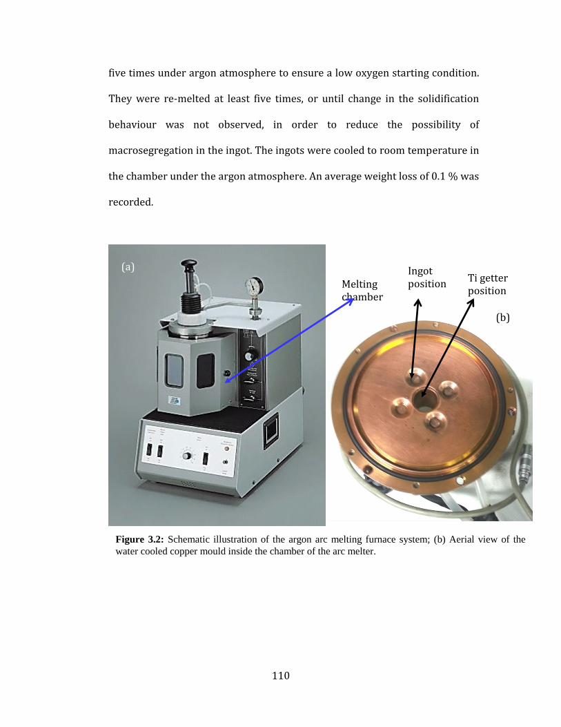
110
five times under argon atmosphere to ensure a low oxygen starting condition.
They were re-melted at least five times, or until change in the solidification
behaviour was not observed, in order to reduce the possibility of
macrosegregation in the ingot. The ingots were cooled to room temperature in
the chamber under the argon atmosphere. An average weight loss of 0.1 % was
recorded.
(a)
Figure 3.2: Schematic illustration of the argon arc melting furnace system; (b) Aerial view of the
water cooled copper mould inside the chamber of the arc melter.
Melting chamber
Ti getter position
Ingot position
(b)

111
3.3.3. Copper die suction casting
The suction casting facility has been incorporated into the argon arc
furnace as a part of the system. As the pre-alloyed ingot was melted in the
argon arc furnace, the melted alloy was pressure induced to suck down onto a
water-cooled copper die under the influence of a negative pressure differential
between the copper die and the melting chamber. The process technique
involves arc melting of 1-20g of the pre-alloyed ingots. This is followed by
forcing superheated molten metallic alloys into the copper die using the excess
pressure in the chamber. The pressure differential is generated by the use of a
roughing pump connected to the secondary chamber at the base of the die
cavity via a solenoid valve. Due to the design of the chamber it was not
possible to measure the actual superheat of the sample, so a successful cast
was strongly dependent on the operator’s judgment. With insufficient
superheat the melt did not completely fill the die cavity. If the sample
superheat were excessive however, the molten metal would access the
secondary chamber and damage or destroy the seal in the solenoid valve.
The chamber of the suction unit is divided in two — the upper and
lower chamber. The upper chamber contains connections for vacuum pumps
(roughing and diffusion), gas inlets (argon is normally used), vacuum gauges
and a tungsten electrode. The lower chamber consists of a water-cooled
copper hearth. The copper hearth has connections for water in and out and for
the secondary chamber, which is controlled by the solenoid valve. The copper

112
block with channels for water-cooling is placed into the copper hearth. In the
copper hearth there is a space where the split die with connections to the
secondary vacuum chamber is fitted. Fig. 3.3 is a photograph of the suction
casting apparatus with a diagonal section of a cupper die in the figure. Several
types of copper dies were employed in preparing the samples. The shapes and
sizes depend on the operator's need. Stepped cylindrical dies with cavities
ranged from 0.5 mm to 5 mm and a conical die with a length of 50 mm and
cone base diameters in the range 2-10 mm were commonly used. The moulds
surfaces were normally polished with 6 micron diamond paste and cleaned
using acetone before use. This was done in order to enhance the thermal
contact between the melt and mould wall and minimise any possible external
contamination of the melt.
The cooling rates of the system had been estimated earlier using an
aluminium composition (Al-4 wt. % Cu alloy). The alloy was suction cast into a
2/3/4 mm stepped die; the cooling rate was then calculated by measuring the
secondary dendrite arm spacing (2) (m), which exhibits the following
relationship with the cooling rate (likely to change with alloy type):
λ2 = 50/Ṫ3 eqn. 3.1
where Ṫ is the cooling rate and 2 is the secondary arm spacing

113
3.4 Microtexture analysis by EBSD technique
In solid crystals, almost every property of interest in the whole
spectrum — ranging from chemical resistance to mechanical properties such
as strength and fracture toughness — is anisotropic.
Furthermore, almost all materials of engineering interest obtained by a
non-specific solidification process (directional growth and single crystal
growth) are polycrystals, which means that they are made up from aggregates
of grains and/or phases.
Predicting the anisotropy of polycrystals from the multi grain/phase
properties involves the fundamental ability to obtain information combining
microstructure and crystallographic studies. This inter-correlated analysis of
the microstructure and of texture, which is non-random distribution of
Figure 3.3: The lower half of the suction casting facility with adjoined picture of a section of a copper die.

114
crystallographic orientations, is called microtexture analysis and it is usually
carried out using Electron Backscatter Diffraction (EBSD) technique.
The EBSD technique, also known as Backscattered Kikuchi Diffraction,
was first developed by Alam and co-workers in 1954 [1], who described some
diffraction patterns and called them “wide-angle back-scattered Kikuchi
patterns” in recognition of related diffraction phenomena reported by Kikuchi
in the 1920s. It was not until the 1970s however that Venerables and co-
workers applied EBSD to metallurgical microcrystallography, paving the way
for a more widespread application of EBSD to the materials science in the
ensuing years [2].
Rapid developments in both hardware and software in the past 10
years have made EBSD an easy-to-use technique, ideal for the rapid analysis of
microstructures in a range of crystalline materials.
3.4.1 Principle of EBSD
This technique allows crystallographic information to be obtained from
samples in the scanning electron microscope (SEM).
In EBSD a stationary electron beam strikes a tilted crystalline sample
and the diffracted electron forms a pattern on a florescent screen. The
specimen tilt angle with respect to the horizontal axis is usually 70 because
this provides the highest yield of backscattered primary electrons. The pattern
obtained is characteristic of the crystal structure, and orientation of the
sample region from which it was generated. The diffracted pattern can be used

115
to measure the crystal orientation, measure grain boundary misorientations,
discriminate between different materials, and provide information about local
crystalline perfection [2-3].
When the beam is scanned in a grid across a polycrystalline sample and
the crystal orientation measured at each point, the resulting map will reveal
the constituent grains morphology, orientation and boundaries.
The principal components of an EBSD system are visible in the figure below
and they can be listed as follows:
SEM station: electronic hardware that controls the SEM, including the beam
position, stage, focus and magnification;
Sensitive charge couple device (CCD): video camera interfaced to a phosphor
screen for viewing the orientation pattern;
Camera control/diffraction pattern processor unit;
Computer and dedicated software to control EBSD experiments analyse the
diffraction pattern and process (data processing and pattern indexing) and
display the results.

116
Figure 3.4: Schematic illustration of the components and assembly of a typical modern EBSD system.
3.4.2 EBSD data presentation
The main standard method of representing texture is by means of
phase map (PM), pole figures (PFs) and orientation distribution functions.
3.4.2.1 Phase map
The sample population can be processed, displayed and quantified
statistically in several ways. The EBSD data processing is usually carried out in
two parts: the orientation map, which represents the more pictorial output,
and the statistical distribution of the orientations.

117
Although the most used application of EBSD is for microtexture, this
technique can also be used for the identification of the phases that compose
the alloy under examination.
The orientation map is a visual portrayal of some orientation related
aspect of the microstructure at each sampling point, accompanied by the
crystallographic orientation. To compose an orientation map, the electron
beam moves automatically in regular steps over a predefined region of
stationary specimen, or, alternatively, the beam is kept stationary and the
specimen is moved. Figure 3.5 is an illustration of an orientation map.
Figure 3.5: Orientation map of the phases which constitute a dual phase material. The
zones coloured blue represent phase A; the red ones represent the intermetallic
compound or phase B; and the yellow zones are the ‘Zero solution’ zones. In the left
bottom angle the marker and the parameter used, for instance the step and the grid, are
also indicated.

118
3.4.2.2 Pole figure
Another common method of representing a microtexture is a pole
figure, which has the advantage that only a single graphic is required to
embody the texture information. To construct a pole figure, the direction of the
plane normal is projected onto a sphere around a crystallite. The point where
the plane normal intersects the sphere is defined by two angles, a pole
distance α and azimuthal angle β. The azimuthal angle is measured anti-
clockwise from the point X (see Figure 3.6).
As the sphere with its pole density is projected onto a plane, this
projection is called a pole figure. A pole figure is scanned by measuring the
diffraction intensity of a given reflection with constant 2θ at a large number of
Figure 3.6: The basis of a pole figure showing the plane normal intersecting with the sphere.
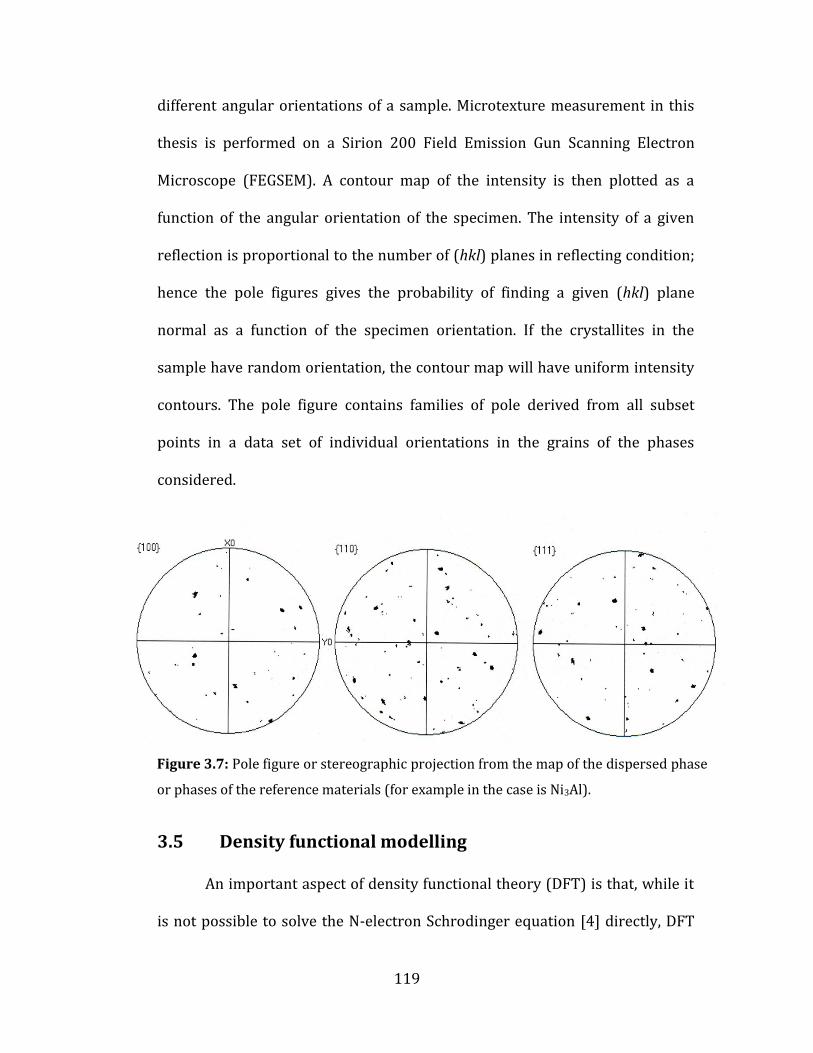
119
different angular orientations of a sample. Microtexture measurement in this
thesis is performed on a Sirion 200 Field Emission Gun Scanning Electron
Microscope (FEGSEM). A contour map of the intensity is then plotted as a
function of the angular orientation of the specimen. The intensity of a given
reflection is proportional to the number of (hkl) planes in reflecting condition;
hence the pole figures gives the probability of finding a given (hkl) plane
normal as a function of the specimen orientation. If the crystallites in the
sample have random orientation, the contour map will have uniform intensity
contours. The pole figure contains families of pole derived from all subset
points in a data set of individual orientations in the grains of the phases
considered.
3.5 Density functional modelling
An important aspect of density functional theory (DFT) is that, while it
is not possible to solve the N-electron Schrodinger equation [4] directly, DFT
Figure 3.7: Pole figure or stereographic projection from the map of the dispersed phase
or phases of the reference materials (for example in the case is Ni3Al).

120
[5-6] gives us, in principle, a method to determine the ground state electronic
structure of a system. This enables materials engineers and scientists to
understand how materials behave under certain physical processes by making
it possible to predict important material properties. On the other hand, due to
the complexities arising from inhomogeneous nature of material’s
microstructure, resulting in anisotropic properties, this problem is not trivial
and an accurate solution is difficult to obtain.
Most metals used in engineering consist of an aggregate of phases. It is
well known that alloy properties are governed by phase content and they
depend additively on the ratio and properties of the constituent phases. The
main difficulty in predicting material behaviour arises from types, sizes and
variations of the phase content due to binary and multicomponent additions
which can interact with each other in a non-linear manner to alter the material
behaviour.
In the late 1980s and early 1990s, Payne and co-workers [7] developed
the CASTEP code for electronic structure calculations. The development made
further enhancement difficult to implement, because there were no modular
structures or written code specifications on it. More accurate developments
and new technologies to redesign CASTEP using a new modular Fortran 90
code were added by a large and disparate number of collaborators and
researchers. Due to the new code re-design, new methods and technologies
are quickly and easily added to CASTEP, allowing users to rapidly take

121
advantage of such developments. The code can be used either in serial or
parallel.
The methodology for electronic structure calculations was
implemented in CASTEP by solving a set of one electron Schrödinger (Kohn-
Sham) equations using the plane wave pseudopotential approach [7]. The
wavefunctions were expanded in a plane wave basis set defined by the use of
periodic boundary conditions and Bloch’s Theorem. The electron-ion potential
is described by means of ab initio pseudo potentials within both norm-
conserving [8] and ultrasoft [9] formulations. Energy minimisation schemes
were used to obtain, self-consistently, the electronic wavefunctions and
corresponding charge density. In particular, the conjugate gradient [7] and
density mixing [8-9] schemes were implemented. The robust electron
ensemble DFT [10] can also be used for systems with partial occupancies (in
particular metals).
Although the total energy is the total quantity, the response of that
energy to external influences is extremely important and can lead to further
direct comparison with experimental data through the calculation of
experimental observables. If the system is perturbed in some way then the
total energy can be expanded as a perturbation series. There is wide array of
physical properties that then become accessible to us; for instance, when a
second order energy is calculated with respect to a given perturbation (see
Table 3.1).

122
CASTEP uses a free form file format so that only the specific commands
required for a calculation need to be given. The set-up tab allows you to choose
the type and quality of calculations that CASTEP will perform, along with other
basic input options such as exchange correlation functional, spin polarisation,
and total energy. The value of all input variables have defaults set, with an
intelligent selection of the essential parameters such as basis size (plane wave
cut off energy) and k- point sets.
Figure 3.8: Graphical user interface of CASTEP available from Accelrys, Inc. namely the materials studio showing 2D pictorial view of a BCC super cell and run geometry optimisation setup.

123
The command line running of the code is simple, with an output file
summarising the details — such as wave function coefficients and charge
densities. This is in addition to the help features.
A graphical user interface is available from Accelrys, Inc.; namely, the
materials studio package which can be used to build the initial structure,
generate input files, run the calculation, and finally analyse the data (see
Figure 3.8). It can be used to create supercells, charge densities, isosurface, to
visualise band structures, and to analyse phonon data among other capabilities.
Some of the task and materials properties that can be calculated using
CASTEP set-up tab include, but are not limited to, the following:
Total energies: Calculation of total energy, forces, stresses and elastic
constants. Electric structure: electric charge densities, orbitals, electrostatic
potentials, band structure, total and partial electronic density of states,
Milliken population analysis, and optical properties (such as reflective,
absorption, refractive index, dielectric, dielectric function) subject to usual
band gap considerations. Previously, through the comparison of predictions to
demonstrate the convergence by running different and larger simulations with
atomic volume between 500 to 5000 Å3 (16-160 atoms) for different
configurations of binary Ti-Nb alloys, we found that an interesting consistency
of linearity exists between the number of atoms per unit cell and the total
energy (ev), as shown in Figure 3.9. Although most published works on
metallic alloys using density functional theory have been based on data from
16 atoms [11-15], the trend from Figure 3.9 suggests that a 64 atoms per

124
supercell adopted in the present study is a good approximation to predict the
properties of alloys that is not likely to differ markedly from the actual ones.
This volume is also reasonable enough to capture the basic physics of Ti-Mo
system.
Geometry: Optimisation of atomic positions and unit cell parameters, either
constrained or unconstrained and external pressure and stresses.
Elastic constant: Performs an elastic constant calculation.
Dynamics: Finite temperature molecular dynamics can be performed under
various conditions such as constant temperature, energy, volume and pressure.
Properties: Calculates properties based on the results obtained from one of
the other tasks; for example, using density functional perturbation theory,
phonon frequencies and eigenvectors are calculated, which can be used to give
the Gibbs free energy, entropy, enthalpy, Debye temperature, heat capacity
and a measurement of phase stability.
Perturbation Physical quantity
Atomic positions phonons
Electric field dielectric properties
Magnetic field NMR
Lattice parameters elastic constants and related mechanical properties
K-point Born charges
Table 3.1: Some examples of perturbation series and physical quantities we can obtain using CASTEP.

125
Figure 3.9: Plot of total energy (eV) as a function of number of atoms per unit cell for different configurations of binary Ti-Nb alloys, displaying the trend of relationship between them.

126
3.6 References
[1] Microtexture determination and its application, 2nd edition — V. Randle — The institute of materials, minerals and mining, Maney Publishing, London UK, 2003. [2] Channel 5 users manual — HKL technology, 2001. [3] http://www.ebsd.com/basicsofebsd 1.htp. [4] Schrödinger E.; Quantisierung als Eigenwertproblem (Erste Mitteilung) Annalen der Physik, (4), 79, (1926), 361-376. [5] Hohenberg, P., Kohn, W.; Inhomogeneous electron gas. Phys. Rev.136 (1964) B854. [6] Kohn, W., Sham, L. J.; Self-consistent equations including exchange and correlation effects. Phys. Rev.140 (1965) A1133. [7] Payne, M. C., Teter, M. P., Allan, D. C., Arias, T. A., Joannopoulos J. D.; Iterative minimization technique for abinitio total energy calculations-molecular-dynamics and conjugate gradient. Rev. Mod. Phys. 64 (1992) 1045-1097. [8] Kleinman, L., Bystander, D. M.; Efficacious form for modelpsuedopotentials. Phys. Rev. Lett. 48 (1982) 1425-1428. [9] Vanderbilt, D.; Soft self-consistent equations including exchange eigenvalue formalism. Phys. Rev. B41 (1990) 1425-1428. [10] Kresse, G., Furthmuller, J.; Efficient iterative schemes for ab initio total energy calculations using a plane wave basis set. Phys. Rev. B54 (1996) 11169-11186. [8] Alfe, D.; Ab initiomolecular dynamics, a simple algorithm for charge extrapolation. Comp. Phys. Commun. 118 (1999) 31-33. [10] Marzari, N., Vanderbilt, D., Payne, M. C.; Ensemble dynsity-functional theory for ab initio moleculardynamic of metals and finite-temperature insulators. Phys. Rev. Lett. 79 (1997) 1337-1340. [11] Chun-Mei Li et al.; First principles investigation of the composition dependent properties of Ni2+xMn1-xGa shape memory alloys, Physics. Rev.B 82(2010) 24201-9.

127
[12] Raabe D. et al.: Theory-guided materials design of multi-phase Ti-Nb alloys with bone-matching elastic properties, Materials 7(2012), 3390/1-19. [13] Ikebata H. et al.; First principles calculations for development of low elastic modulus Ti alloys, Phys. Rev B 70 (2004) 174113/1-8. [14] Dai J. H. et al,; Electronic structure mechanism of martensitic phase transformation in binary titanium alloys, Appl. Phys. 112 (2012) 123718/1-9. [15] Rodriguez A. J., Mailti A., Brito L. J.; Phase transformations and electronic properties in mixed-metal oxides: Experimental and theoretical studies on the behaviour of NiMoO4 and MgMoO4, J. Chem. Phys. 112, (2000) 935; doi: 10.1063/1.480619.

128
Chapter 4
A Modelling Approach to Property Prediction in
Metallic Alloys
4.1 Introduction
The phase transformations which can occur in binary titanium and
other 3d (such as Zr and Hf) metals with elements such as Nb, V, Fe, Mo and Cr
form an area of exploration for physical–chemical factors of structural
stability. This is largely because, while they possess a BCC solid solution
(called the β phase) extending over large composition ranges at high
temperatures, metastable phases are formed during the decomposition of β
phase, which has a marked effect on the physical properties of these alloys. For
example: several forms of martensite have been observed in titanium alloys
after transformation of the high-temperature BCC form of titanium to HCP (1-
9), orthorhombic (9, 10), and FCC (8) or FCT (5, 6) structures.
In the Ti-Mo system specifically, it has been shown that hexagonal
martensite is formed in alloys containing up to approximately 4% Mo and that
orthorhombic martensite is formed in alloys containing between 4%- 8% Mo
(9), which has a space group of Cmcm (No.63) and lattice parameters of a=
3.01Å, b=4.91 Å, and c=4.53 Å. The lattice parameters do, however, vary with
alloy compositions [11]. The Ms is below room temperature for alloys that

129
contain greater than 10% Mo and thus remain single-phase BCC on water
quenching.
Traditionally, materials scientists have studied the structure of the
metals and alloys relying mainly on phase stability phenomenon to account for
the material properties. Early studies focused on the explanation of trends in
the periodic table, such as the sequence of structures HCP → BCC→ HCP → FCC
that is observed when going from left to right across the transition metal (TM)
series [11-16]. This is a formalism based on the thermodynamic description of
trends in terms of energy difference of equilibrium structures as a function of
electron per atom, (e/a) or in some literatues as Ne [14]. Following the trend,
most theoretical [11-20] and experimental [21-23] studies on the
development of engineering alloys that exist in the literature are usually based
on the properties of the equilibrium phases such as BCC or HCP.
Interest in the study of complex and metastable phases and their
relationship to materials properties has been rekindled by recent
developments and an increasing complexity of industrial materials designed to
meet the demand for high-tech applications. Such interest requires more than
the aforementioned approach. Nevertheless, while there is a huge interest in
equilibrium structures such as BCC, FCC and HCP of metals and alloys that are
well understood, this specialisation, while no doubt necessary, carries the risk
that more complex metastable phases that occur in binary and higher order
metals and alloys have been neglected.

130
It should be noted that complex metallic alloys have come into
increasingly widespread use and engineering and scientific interest in these
materials is growing continuously. The physical essence of the processes that
take place in these alloys is, however, still not well understood. Both an
improvement in the mechanical properties of metallic materials and their
physical stability are critical to further progress in the field of their research,
development and use. It is therefore of great value to further explore the
structural relationships of some of these alloys by examining for related
phases and their corresponding properties. Ti–Mo alloys are most widely used
as superconducting materials, and also find uses in aerospace applications [25,
26], petro-chemical and biomedical industries. It is therefore important that
the relative phase stability in this system is understood properly. In titanium
and related alloys, there has been a considerable amount of discussion
concerning the unique physical and chemical properties of orthorhombic
martensitic () phase [25]. The role of phase for the shape memory effect
and psuedoelasticity phenomenon, as well as the reduction of Young’s
modulus for biomedical titanium based alloys, is well known [27-28], but the
theoretical information including investigations pertaining to competing phase
transformations between β → martensites (, ), thermodynamic stability,
mechanophysical and electronic properties with respect to the usual TM
structures such as Mo, Nb etc., is unknown. Certainly, this lack of information
limits understanding of the general trends in the properties of Ti and other 3d-
TM alloys. This is why we consider orthorhombic martensitic () in the

131
present work a representative example of complex binary phases derived from
or combining with the initial BCC structure to form a multiphase alloy.
The present study has three main objectives. The first is a general
objective to build theoretical understanding of the metastable orthorhombic
() martensitic structure in the Ti-Mo alloy systems. To this end, first
principle calculations based on the density-functional theory (DFT) and using
the commercial version of Cambridge Serial Total Energy Package (CASTEP
code) method will be performed, on the basis of which a detailed analysis of
the predicted structural properties will be compared with some experimental
data.
The second objective of the work is to study the thermodynamic
stability of the orthorhombic () martensitic relative to BCC structure (i.e. the
structure from which forms in the Ti-Mo alloy systems) by quenching in
alloys. More specifically, we shall first construct and compare a Gibbs free
energy G obtained through the structural energy difference (SED) versus ne
plot, and then use it to obtain information on the β→ phase transformation.
Based on this, a microscopic picture of the stability based on the band filling
of electron bands will be developed.
The third objective of the work is to use information provided by
homogenising the elastic constant BCC and orthorhombic crystal structures in
the way described elsewhere [29] to predict the polycrystalline elastic
property of the alloy. In this way a good comparison will be made with

132
previous experimental data, and additional insight gained into the stability of
the BCC phase in 3d-TMS alloy systems.
4.2 Experimental and theoretical methods
4.2.1 Calculation details
All the calculations in this study are based on the electronic density-
functional theory (DFT) implemented using the commercial version of
Cambridge Serial Total Energy Package (CASTEP code) method [30]. In this
code, the Kohn-Sham [31] single electron equation model with periodic
boundary conditions and the psuedopotential method as an approximation of
the atomic core-valence electron interaction, as well as the electronic wave
function with kinetic energy smaller than a specified cut-off energy cut-off, are
expanded in a plane wave basis.
The exchange and correlation are treated using the generalised-
gradient approximation (GGA) of Perdew, Burke and Ernzerhof (PBE)
formalism [32] due to its computational efficiency. The motivation for our
choice is that the (PBE) methods are efficient, due to their accuracy in
describing the bulk properties of many materials, and flexible enough to
describe the random distribution of the impurity of atoms on Ti lattice [28].
The PBE functional is designed to reproduce closely the PW91 results, but the
PBE formulation is more robust to guarantee a high level of convergence, cut-
off energy of 500 eV and the Methfessel and Paxton [19] Gaussian smearing
method with 0.1 eV smearing of the electron levels.

133
We studied 16 different binary Ti-Mo materials (eight each for
orthorhombic () and body-centred cubic (β) phases). For each structure,
tests were carried out using different k-point meshes to ensure absolute
convergence of the total energy to within a better than 1.0 meV/atom. For all
structures considered, we calculated the total energies as a function of volume
while optimising unit cell-external degree(s) of freedom (i.e. the unit-cell
shape) and unit cell-internal degree(s) of freedom (i.e. Wyckoff positions) as
permitted by the space-group symmetry of the crystal structure. Such
structural optimisations were iterated until the Hellman–Feynman forces were
less than 4 meV/Å in magnitude, ensuring a convergence of the energy with
respect to the structural degrees of freedom to better than 1 meV/atom ( 0.1
kJ/mol). In addition, all calculations were performed using the ‘‘accurate’’
setting within CASTEP code to avoid wrap-around errors. With the chosen
plane-wave cut-off and k-point sampling, the reported formation energies are
estimated to be converged to a precision of better than 2 meV/atom.
For alloying systems, one titanium atom was substituted by an alloying
atom in each supercell, and the relative concentrations of alloying elements in
the systems ranges from 3 to 23 at.%. A random distribution of the chemical
species over the sites of the structures has been considered and studied by
replacing Ti atoms by Mo atoms (as illustrated in Figures 4.1 and 4.2),
representing different Mo concentrations for BCC and orthorhombic
structures respectively.

134
The equilibrium phase boundaries and the phase transformations
which occur in titanium systems can be rationalised using a thermodynamic
approach. In particular, some insights can be gained into metastable
transformations which can be expected where experimental data are lacking.
It is known that the orthorhombic crystal structure is not stable in
molybdenum, niobium and vanadium. The fundamental quantity expressing
the thermodynamic stability of an alloy is the alloy formation energy. The
formation energy (per atom) of and β phases in binary Ti-Mo( where =
3,6,8,9,10,14,18,23) in configuration = BCC/HCP is defined as:
(
( ). ) (4.1)
Here, N is the total number of atoms per supercell, is the first
principle calculated total energies of the respective alloys; µ is the chemical
(a) (b)
Figure 4.1: The 4x4 32 atomic supercell of (a) a BCC crystal structure; and a 2x2x2 32 atomic supercell of (b) an orthorhombic martensitic crystal structure both from the closed packed [111] plane of (Ti-Mo) used in the calculation, with the atoms numbered (1-6) variably in the various atomic layers (depicted in two distinct colours for Ti and Mo in the two supercells by large spheres for the sake of clarity) in the [111]β and [0001] directions.

135
potential of the element Ti or Mo in its corresponding bulk phase, respectively,
and x the alloy composition. In the above definition (Eqn.4.1), the alloy is
thermodynamically stable for . From the point of view of
thermodynamics, lower formation energy means better stability of a particular
crystal structure over another.
Past studies [20-23] revealed deformation of metastable β Ti alloys can
lead to the formation of stress-induced martensites (SIMs), and the reversion
is the basis for the shape memory and pseudoelastic effects. G is more
descriptive than the total energy, which includes a large contribution from
states that do not play a role in bonding. In order to gain some insight into the
activation energy for SIM transformations in β -Mo alloy, we performed total
energy calculation using DFT-GGA implemented on the CASTEP code to
determine the free energies G of and β structures for Ti-Mo using Eqns.
4.2 and 4.3 respectively.
⟨
n n
⟩ .
⟨
n n ⟩ . .
Here ,
and
represents the excess free
energies of mixing in terms of the pure β / titanium element, pure β /
Molybdenum element and the bulk with different phase configurations, but
with the same concentration of Ti-Mo system and R=(8.314)/KMol. At
equilibrium in the two phase (β + ) region of the phase diagram:
136
(4.4)
For a given alloy, and are the atomic fractions of solute at the limit of
solubility. This allows the determination of free energy of any composition.
For many applications, the study of elastic response is of critical
importance. Not only does it provide the measures of the deformations under
loading, but from a microscopic viewpoint the elastic constants provide an
accurate measure of the strength of the average interatomic bonding and
therefore insight into related expected such as hardness [3, 25].
In the present study, to obtain the integral elastic response of
multiphase polycrystalline samples we followed the procedure originally
applied by Zeller and Dederichs et al. [33] to determine elastic properties of
single phase polycrystals with cubic symmetry. This work was later
generalised and further extended by Midada and Basu et al. [33,34] and by
Raabe et al. [20] to multiphase composites to determine: (i) the elastic single
constants, and (ii) the volume fraction of the components within a self-
consistent T-matrix solution for the effective medium. The T-matrix approach
is based on the multiple scattering theory. It can be reviewed in terms of a
macroscopic homogeneous effective medium consisting of microscopic
fluctuation characterised by an effective stiffness defined by:
⟨ ⟩ ⟨ ⟩ (4.4)
Here, is the local elastic constant tensor with ⟨ ⟩ and ⟨ ⟩ as the
local stress and strain field at a point r, respectively, and the angular brackets
denote ensemble averages. A repeated index implies the usual summation

137
convention. The effective stiffness is defined by:
⟨ ⟩ ⟨ ⟩ (4.5)
Since the aggregate represents a body in equilibrium, | where
| ⁄ and the local elastic constant tensor can be now be decomposed
into an arbitrary constants part ( ) and a fluctuating part — .
(4.6)
As shown in [33], an integral part of Eqn. 4.6 is the interactive equivalent
solution representing the resulting local strain distribution (in a short
notation) as
(4.7)
Here, and G are the strain and modify Green’s function of the medium
defined by , and the T-matrix is given by:
, (4.8)
Here, І is equivalent to the unit tensor. Combining Eqns. 4.2 and 4.4, we get
⟨ ⟩ ⟨ ⟩ ⁄ (4.9)
Although Eqn. 4.6 constitutes an exact solution for , finding the exact
solution of ⟨ ⟩ and ⟨ ⟩ for realistic cases is impossible. By neglecting the
intergranular scattering that may occur in some cases in the form of grain to
grain position orientation correlation function however, the T-matrix can be
written in terms of single-grain t –matrix ( ) for each grain
∑ . (4.10)
where
(4.11)

138
with
∑
Inserting Eqn. 4.7 into 4.6 leads to:
⟨ ⟩ ⟨ ⟩ (4.12)
For single phase polycrystal, the self–consistent solution of Eqn. 4.12 can be
obtained by choosing a that satisfies:
⟨ ⟩ (4.13)
For a multiphase polycrystal, a solution to Eqn. 4 can be found by evaluating
the volume fraction and of each phase respectively [33] via
⟨∑ ⟩ (4.14)
The application of the method to both single-phase aggregates and multi-
phase composites relevant to Ti-Mo alloys is as follows.
4.2.1.1 Single-β phase aggregate
For a single-phase polycrystal with cubic symmetry [33, 34] to the
following expression for and
( ) =0 (4.15)
In Eqn. 4.12, three independent single crystal elastic constants —
— define the single crystal bulk modulus
⁄ , the
tetragonal shear modulus ⁄ and trigonal shear modulus, ,
⟨ ⟩
.
For polycrystals with orthorhombic symmetry, Eqn. 4.10 and 4.11 are reduced

139
to a set of coupled equations for and .
(4.16)
(
)
(4.17)
where
(4.18)
⁄
(4.19)
⁄ (4.20)
; (4.21)
(4.22)
- ; (4.
23)
(4.24)
(4.25)
(4.26)
(4.27)
(4.28)
⁄ ⁄ (4.29)

140
⁄ (4.30)
and orthorhombic symmetry has nine of the single crystal elastic constant;
namely, and .
4.2.1.2 Multi-phase (β/) aggregate
The elastic constants of a multi-phase polycrystal can be determined directly
by coupling 4.10 for and the components of the T-matrix. For
materials with cubic symmetry, the equation is defined by:
(
)
(
)
(4.31)
(4.32)
where β is defined in Eqn. 4.25 with and replacing and . For
materials with orthorhombic symmetry, the equation reads:
( )
(
)
(4.33)
( )
[ ( )
]
(4.34)
Here, β is defined in Eqn. 4.33, is defined in 4.34, and in Eqn. 4.33. Here,

141
again and replaces and in the equations for β, , and .
4.2.1.3 Homogenised Young's modulus and Poisson's Ratio
As soon as and have been determined, the homogenised Young’s
modulus ( ) and Poisson’s ratio for (an elastically isotropic) polycrystal
can be determined using standard elasticity relationships. The homogenised
polycrystalline Young’s is calculated using:
(4.35)
— and the homogenised polycrystalline Poisson’s ratio is calculated using
(4.36)
4.3 Experimental methods
4.3.1 Materials
In order to compare the prediction with experimental data, five different
compositions of Ti-Mo alloys were made. The alloys were prepared from
99.9% pure titanium and pure molybdenum in an electric arc-melter under an
argon atmosphere into buttons containing approximately 10 grams, at the
Department of Materials Science and Engineering University in the United
Kingdom. (The actual chemical compositions have been summarised in Table
4.1, and all compositions are in atomic percentage — hence percentage will be
mentioned instead). The furnace was equipped with a water-cooled copper
crucible. The temperature of the electric furnace amounted to about 3000⁰C,
while the melt was at the electrode centre-hold peak temperature that is above

142
2050⁰C in order to ensure complete dissolution of the solid Ti and Mo metals.
To ensure optimal chemical and structural homogeneity, each button
was remelted and turned over six times in order to eliminate dendritic
structure, and the final ingot was cast into a cylindrical sample of ≈90 mm in
length and 8mm in width. This led to rapid solidification and suppression of
dendritic formation. The copper mould had a temperature of about 20⁰C,
which led to rapid solidification and suppression of dendritic formations. All
the cast samples were subjected to homogenisation in quartz tubing at 1200ᵒC
in an argon atmosphere for five hours in to remove microsegregation. These
samples were quenched in water. These samples were only superficially
contaminated. Before characterisation of the microstructure, the surfaces were
cleaned by mechanical polishing followed by electropolishing in a solution of
five glacial acetic acid and acetone, since Ti alloys undergo strong chemical
reaction with oxygen,
Alloys Mo O N Ti
Ti-6Mo 6.3 0.07 0.013 bal.
Ti-10Mo 10.2 0.05 0.005 bal.
Ti-14Mo 14.16 0.06 0.007 bal.
Ti-18Mo 18.08 0.07 0.002 bal.
Ti-20Mo 20.12 0.09 0.002 bal.
TI-23Mo 23.3 0.08 0.005 bal.
Table 4.1: Nominal chemical composition of Ti-(6-23) Mo alloys (unit: atomic %).

143
4.3.2 X-Ray measurements and Microstructure analysis
Phase constitution was investigated using XRD diffuse scattering
measurements at room temperature with monochromatic CuK and radiation
diffracted from a bent silicon crystal cut to the (111) orientation. The detecting
assembly consisted of a proportional counter and a pulse height analyser
arranged to eliminate the one-third wavelength of the white radiation (the one
half component was eliminated by the silicon crystal), the cosmic background
and the fluorescence radiation from titanium. Readings were recorded
continuously on a horizontal spectrometer with the counter rotating at 0.25⁰
in 2Θ/min, and measurements were made from 10 to 100⁰ in 2Θ. Flat samples
were used and the geometry of the system satisfied the usual focussing
condition.
For the quantitative phase, an analysis was performed with an X’Pert
Highscore software package. Chemical etching was done for optical
microscopy using a solution of 15% HCl, 8% HNO3 and 77% H2O (distilled
water). The microstructure was cross examined using electron backscatter
diffraction (EBSD) after grinding on 400, 600, 1200 and 2400 paper with
subsequent use of 6m (35min), 3m (20min), and 1m (15min) polishing.
4.3.3 Measurement of modulus of elasticity
This basic material property is of interest in many manufacturing and
research applications and is related to the atomic bonding of the materials. In
the case of biomaterials for load bearing applications, the elastic modulus is an

144
important parameter. The stiffness mismatch between implant material and
surrounding bone leads to ‘stress shielding’ of the bone. Higher stiffness or
Young’s modulus of the implant will result in a greater amount of bone loss,
bone fracture and loss of bone interface. Loss of bone due to stress shielding
effects also makes revision surgeries more difficult. Finite element analysis has
suggested that a low elastic modulus hip prosthesis can stimulate better bone
growth by distributing the stress to the adjacent bone tissue [20]. The elastic
modulus of the materials can be determined by different methods, such as
ultrasonic technique.
Velocity of the ultrasonic waves in a solid medium is directly related to
the elastic properties and density of the material. The elasticity of the material
delays the transmission of wave and introduces a time delay, i.e. a phase lag.
When the frequency of the wave is higher than the audible range, it is called
elastic wave or ultrasound. Two types of vibration-induced deformation
resulting in compression or shear are generally possible in an infinite medium.
These are associated with two modes of elastic wave propagation, i.e.
longitudinal waves, where particles are displaced along the direction of
propagation and transverse or shear waves, where the particles are displaced
perpendicular to the direction of propagation. The velocity of propagation of
the elastic waves in a body is characteristic of the material [32].
Ultrasonic waves are generated in the material by a transmitter
oscillating at the desired waveform and frequency, with collection by a
detector. Ultrasonic velocity changes have been determined by time-of-flight

145
measurements using Olympus 6.2 ultrasonic equipment. The relationships
between ultrasonic velocity and the elastic properties of materials are given
below [33–35].
Young’s modulus (E) is expressed as:
(
)
(4.37)
Shear modulus (G) is the ratio of shearing stress τ to shearing strain γ within
the proportional limit of a material and is expressed as:
(4.38)
Poisson’s ratio υ is the ratio of transverse contraction strain to longitudinal
extension strain in the direction of stretching force and is expressed as:
(
)
(4.39)
In the above set of equations, VL and VS are the ultrasonic longitudinal
and shear wave velocities, respectively, and ρ is the density of the material.
The elastic modulus of the samples was measured by ultrasonic method on an
ultrasonic velocity gauge, Olympus 62, UK. A normal incident probe (model
M110, 5MHz) and a shear probe (model V221, 5MHz) were used for the
measurement of normal and shear velocities of the wave, respectively. The
density of the samples was measured using an automatic meter; for each
composition at least five samples were measured.

146
4.4 Results and discussion
4.4.1 Structure and interatomic bond distances
4.4.1.1 Definition and crystallographic considerations
The orthorhombic phase can be described as a type of martensitic
structure formed by the stretching of the BCC lattice along two of its
orthogonal pairs when the constraints to form hexagonal or body-centred
cubic structures cannot be met. In essence there is a contraction of "c" axis and
stretching of “a" and "b" axes with the collapsing of the inner atoms into the
same plane with distinct angles a, b and c. This permits a continuous
transformation of → β transformation, as the stability of the transforming
matrix is increased. The atomic positions are (0, y, 1/4), (0, , 3/4), (1/2,
y+1/2, 1/4) and (1/2, +1/2, ¾). In Figure 4.2 we see a partial view of the two
structures along the “c” axis of the unit cell, further illustrating the
transformation of both phases. The orientation relationship between the
original β and the sheared orthorhombic phase has been established
approximately as (0110) β(001)″ and [111]β[101]″.

147
4.4.1.2 Symmetry and bonding strength/length of and β phase
Ti-Mo is a compound based on elements in group IV and V of the
periodic table. As Mo (2.16) is significantly more electronegative than Ti
(1.54), the Ti-Mo bond is partially ionic. In effect, one of the main differences in
the crystal structures of the BCC (β) and phases of Ti-Mo might be the
changes in the interatomic bond distances with alloying additions. We
performed ab initio calculation of the total energy and electronic structure in
the present work using the DFT-GGA method [30, 32, 33] to determine the
interatomic bond distances of the metastable and stable β phases for Ti-
Mo alloys (where = 3, 6, 8, 10, 12, 14, 18) for a system with the external
pressure P=0. Indeed, Table 4.1 shows that in the three interatomic bond
Figure 4.2:(a) Unit cell of (a) orthorhombic (b) BCC phase; and (c) scheme of the geometrical relations between the [001] projection of orthorhombic and BCC phases, the atoms that are involved in the formation of the BCC phase are shown in red filled circles while the orthorhombic corner atoms are blue open circles.
(b)
(a)
c
cβ
bα
bβ
α
(c)

148
lengths (IBLs) of the and β phases, two atomic types can be identified. The
first corresponds to metal atoms that occupy mixed Ti-Mo-Ti or Mo-Ti-Mo
rings. The second type includes metal atoms that are in pure Mo-Mo or Ti-Ti
rings. Implicitly, Mo atoms can form two types of bonds: those that bridge the
chain of rings and have only two Ti neighbours, and those that form part of the
rings and have three or four neighbours. Within the rings, one can have metal
bonds that are either parallel or perpendicular (Ti-Mo, or Mo-Mo, Ti-Ti).
Essentially, one has a stack or column of three membered titanium-
molybdenum rings.
From Table 4.1 ( phase), we can see that the coordination of Mo-Mo
(2.770 Å) is substantially longer than typical Mo-Mo bond length (2.725 Å)
[37]; while in the Mo-Mo bond d stances n β-Ti-Mo are close enough to allow
substantial Mo-Mo interactions. The indication of non-Mo-Mo bond interaction
at Ti-3% and Ti-6% as observed in Table 4.1 can be ascribed to seemingly
strong Ti-Ti bonds in the lean Mo concentration range [38] (see Table 4.1).
These strong Ti-Ti interactions disappear, however, when the Mo-Mo
d stances are abr dged to produce the β-phase.

149
In Figure 4.3, we plot the interatomic bond distances (IBD) of Ti-Ti
for and β phases as a function of compositions. For the α structure (black
dots), we can see from figure 4.3 that the Ti-Ti bond distances in the crystal
structure increased in the lean Mo alloy where the occurance are highly
probable, but were mainly unchanged in high Mo region. In the context , the
distortion of phase leading to orthorhombic martensitic structure in the
lean Mo region in Ti-Mo system can be interpreted as a way of keeping the Ti-
Ti bond distance unchanged, in spite of the fact that the lattice parameter of
the structure varies with composition. A possible explanation of this result
has been proposed [38], suggesting that certain sites might be fully occupied
Initial crystallographic dimensions (Å) aβ = 3.2 a″ . b″ . c″ .
Alloys [at.%]
3 2.8679 2.8679 2.6948 2.6281 -
-
6 2.8733 2.8833
2.7029 2.6945 - -
8 2.875 2.8750 2.7156 2.7156 2.7704 2.7704
10 2.8769 2.8799
2.7135 2.6848 2.5650 2.7435
12 2.881 2.8721
2.7006 2.7006 2.7870 2.7370
14 2.8819 2.8690 2.6971 2.6971 2.7084
2.7084
18 2.882 2.8679 2.7007 2.7007 2.6949 2.6949
Table 4.2: The ratios between interatomic bond lengths (IBLs) of α and β phases for Ti-Mo calculated by DFT-GGA calculations.

150
by Group 1V atoms, which due to seemingly strong Ti-Ti bonds keep the
in Ti alloy identical to that of pure elements [40]. They found that the Ti atoms
are distributed amongst the A-type and B type sites in an essentially random
fashion.
For the β-phase, Figure 4.3 (the red line) clearly illustrates that the Ti-
Mo interatomic bond remains essential for the change in the crystal structure
of the Ti-Mo alloy. Molybdenum atoms produce major structural perturbation
in the unit cell of Ti-Mo to force the breaking of the Ti-Ti bonds and the
format on of β -Mo alloy.
A possible explanation for the change in crystal structure from →β
was offered by Brown et al. [9]. In the orthorhombic martensite of Ti-Nb
Figure 4.3: The composition dependence of Ti-Ti bond distance for and β phase according to the present work. The lines are only to guide the eye.

151
system they found no evidence of segregation of niobium to special sites, and
showed that the crystal structure gave an eightfold co-ordination around each
(Ti, Nb) atom, with four additional neighbours at a slightly greater distance.
Both atoms have a Goldschmidt atomic radius of 1.47Å and, therefore,
difference in size is unlikely to account for the distortion to orthorhombic
symmetry alone. It was suggested that the distortion was a reflection of a
tendency for niobium to retain the eightfold co-ordination obtained in the BCC
form.
Similarly, crystal structure transition in the Ti-Mo with rising Mo can be
regarded as a change in the nearest neighbour co-ordination from twelve in
the HCP structure to approximately eight in the orthorhombic structure and
eight in BCC. The size of molybdenum (1.36Å) is very close to that of titanium,
and size difference affects should again be small. This was noted by Dupouy
[41] of Ti-Ti and Mo-Mo atomic bonds tending to approach the average
distance in the solution at compositions of between 10 and 50 at.%
molybdenum, and was taken to indicate an electron exchange in the solution.
The present results are consistent with the above suggestions for the
change in →β symmetry. One can therefore bel eve that the ma ma could
be accidental or could be a clue to the role that Mo plays n stab l s ng β-Ti
alloys. Thus, leading to the mpl c t trans t on states for → and →β
structures respectively, where Ti-Mo bonds reorganise within the unit cell and
the system gains stability by adopting the new phase, which corresponds to
the new structures — as illustrated in Figure 4.2(c). Figure 4.4 is thought to be

152
a successful illustration of the legitimacy of all the above statements.
4.4.1.3 Lattice parameter
An interesting conclusion follows from the comparison of the
theoretically lattice constants of the optimised Ti-Mo alloy structures and the
as water quenched Ti-Mo alloys experimental analysis of the X-ray diffraction
patterns, shown in Figure 4.4(b). The calculated lattice parameter decreases
linearly with the excess Mo concentration. The x dependence of the theoretical
lattice constant can be fitted as . . , which is in good
agreement with experimental relationship, . . . Note that
the theoretical experimental is only about 0.1% smaller than experimental
value.
The decrease in the lattice constant with increasing x can be attributed
to two factors. One is that the atomic radius of the Mo (1.36 Å) is slightly
smaller than that of Ti (1.46 Å). The replacement of Ti by Mo therefore induces
the shrinkage of the crystal lattice. The second factor was a change in the
nearest neighbour co-ordination from approximately eight in to eightfold
co-ord nat on n or g nal B β cell wh ch means the distortion is a reflection
of a tendency for molybdenum to break Ti bonds and retain the eightfold co-
ordination obtained in the BCC form, resulting in a reduction in the lattice
parameter.
The lattice contraction by about 5% that is reached in Ti-Mo in
compar son w th pure n t ates the ″ β transformat on s m lar to the
appearance of phase under pressure in Ti. Further lattice decrease in

153
ternary alloys on the Ti-Mo bas s favours β-phase and low Ms.
It is our belief that the ″ phase appearance n β phase alloys of w th
Mo, Fe, Nb, Mn, Cr and V can also be considered the result of lattice parameter
contraction. The analysis shows that ″ phase n β-phase alloys appears at
electronic concentrations 4.09~ 4.16 and lattice parameter 3.225 A. The
analysis from theory was consistent with the experimental behaviour of more
recent values for Ti-Mo alloys obtained [9], probably due to the large basis-set
employed in the present work. The minor discrepancy between experimental
results may be due to differences in temperatures, or probable approximations
inherent to DFT-GGA [22, 23] may play a role.
Figure 4.4: A comparison of the theoretical and experimental determined lattice parameter of the alloys in to the present work. The lines are only for guides to the eye.

154
4.4.2 Energetic analysis of thermodynamic stability – ab initio
simulation
4.4.2.1 Thermodynamic analysis of and ″ stability in Ti-Mo alloy: theory
In order to compare the relative stability of β phase w th respect to ″
phase stability, the formation energies for and structures in Ti-Mo
system, at T= 0K formation energies have been calculated based on Eqn. 4.1.
The result of the relative stability between the two phases as functions of Mo
content is shown in Figure 4.5. As can be seen in Figure 4.5(a), which shows
format on energ es of ″ and β phases the two phases closely track one
another. While the formation energy of phase is slightly more negative
(exothermic) in low solute alloys (3 at.% to 8 at.% Mo), Mo destabilises the ″
phase format on energy ncreases w th compos t ons but stab l ses the β the
formation energy decreases with compositions). The present results are
consistent with other studies [6, 9, 21- ] on β-Ti-Mo alloys, and this
consistency in also obtained in the Ti-6% Mo alloy. The estimated energy
difference is 3.5 eV between ″ and β phases wh ch s close to other
theoretical reports of 2.9 eV [20, 23, 24], and slightly larger than another
estimation [23]. The difference between the formation energies of the two
phases, however, is 3.5 eV/atom. This indicates their nearly equal
probability to occur in the samples. Again, the process of β″ transformat on
is associated with small strain, which is less than β transformation. The
small strain might account for the β″ transformat on ahead of β or as

155
explained elsewhere [24]. We found the influence of site occupancy rather
weak.
Figure 4.5: (a) Theoretical alloy formation energy at T=0K; and (b) free energies of formation at 20⁰ C (293K). The results are displayed as a function of composition, the region in between the dotted lines depicts the most likely region of coexistence of both phases. The lines are to guide the eye.
4.5(a)
4.5(b)

156
On thermodynamic stability, it should be noted that these calculations
found negative formation energy for both phases in agreement with
calculations by Rudman [42], who determined values for the heat of mixing of
Ti-Mo alloys using a bond-energy concept. For an alloy to be
thermodynamically stable, its formation energy must be negative. According to
Figure 4.5(a), ″ and β structures exhibit similar behavioural path ways in Ti-
Mo alloys. For phase, the formation energy at temperature T=0K is more
endothermic at a low Mo concentration of between 3 at.% — <8at. %. Mo is
thermodynamically immiscible in phase in a low concentration regime. It is
only reasonable that ″ phase will be the more stable phase even without any
entropy stabilisation effects.
In contrast, β phase at the T=0K is very stable beyond ≈ 8 at.% Mo. The
significance of this result is that Mo is completely immiscible in β phase at ≈ 8
at.%. We can conclude from this result that ″ is very unstable at higher Mo as
it promotes β stability at high concentration regimes even in the absence of
any entropy driven temperature effect.
In view of the practical application of biomedical Ti alloys, we felt that
ambient temperature is a more suitable choice as a reference temperature for
the formation and stabilisation of both phases. The corresponding results are
shown in Figure 4.5(b). The results as shown in Figures 4.5(a) and 4.5(b)
confirm earlier reports [20] suggesting that the energy spread for given
composition in Ti alloys and the different local configurations are weak, and
that their dependence on energy of formation are also lacking. Hence, the small

157
and negative interaction parameter obtained in the result is well justified.
Although the effect of temperature is less pronounced, evidently the
finite temperature significantly reduced the formation energy, thus indicating
the stability of the alloy is somewhat entropy driven. A direct comparison of
the outcome of this theoretical result with experimental results based on the
first occurrence of a stable fraction of ″ and β phases can now be done.
4.4.2.2 Thermodynamic analysis: comparison of the theoretical
predictions and experimental data
The onset of β phase formation, its composition and volume fraction
can be described using the hypothetical free energy composition, following the
work by Raabe et al. [20] on HCP and BCC in T-Nb and Ti-Mo systems. We
therefore predicted these by performing a Gibbs construction using the
average formation energy to compare the experimentally determined onset
and volume fraction of the β phase for the alloys. The Gibbs construction was
performed by approximating third-order polynomial using a least-squares
approach because of the important statistical interpretations. The actual Gibbs
construction and the volume fraction of the ″/β phases are summarised in
F gure . a . he G bbs construct on found at.% Mo as the threshold
concentrat ons where only β-phase exists. The result of calculated volume
fractions of the phases are summarised in Table 4.3, shown in the blue circle in
Figure 4.6(b).
In order to compare the experimentally determined volume fraction of

158
the two phases, we conducted x-ray wide angle diffraction experiments on the
Ti-Mo alloys associated with the region of interest — see Figure 4.6(c). The
splitting of the diffraction profile lines for the Ti-6% and Ti-7% alloys as a
result of an increased orthorhombic distortion is in agreement with the
theoretical prediction ″ phase reg ons for th s system. o further ver fy th s
prediction, the phase content of as quenched Ti-18 at.% Mo alloy determined
by x-ray diffraction was further cross-examined by the EBSD measurement
(see Figure 4.6d). The indexing of this EBSD image reveals a random texture of
almost complete BCC structure with an isotropic grain shape.
As e pected because Mo s a h gh β stab l ser the results of the G bbs
free energy detailed in the present work entails that the alloy has a narrow
two-phase ( β w ndow. Furthermore appl cat on of the lever rule to the
tangent of the ″ and β curves shows that n agreement w th H ckman’s
findings [44], the volume fraction of ″ decreases w th ncreas ng alloy
content. The overall form of the Gibbs construction from formation energies
suggested here, however, indicates the existence of a metastable orthorhombic
martensite in Ti-Mo system, and the phase diagram should include either a
monotectoid reaction or a metastable miscibility gap within the ( β phase
region.

159
Figure 4.6(a) Gibbs construction and (b) volume fraction of the β phase of Ti-Mo alloy are shown. The volume % of β phase as determined by DFT calculation method is shown by (black) crossed block, while the red crossed circles are experimental determined volume %. The red arrow marked the threshold concentration for single β phase of the alloys. The error bars fall with the symbol size.
Gib
bs
free
en
ergy
co
nst
ruct
ion
(eV
/at)

160
Figure 4.6 (c) For comparison, the indexed diffraction spectra from XRD scanned from 30 to 80 degrees in diffraction angle, revealing reflections due to the phases for the of Ti-Mo alloy, (where = 6,10,12,15, 18 at. %) reveals the phase structures; (d) EBSD image of the experimental observed microstructure of Ti-30Mo. The EBSD image reveals an isotropic grain shape and a random texture. Colour code; miller index in standard triangle of lattice directions pointing in normal and casting direction.
(d)
Ti-18Mo

161
4.4.3 Elastic modulus and phase stability
Having determined the thermodynamic stability behaviour, let us now
focus on predicting and comparing the elastic properties determined from the
first principle total energy calculation and experiment. This is not trivial,
however, since the exact distribution of Ti and Mo atoms over the lattice
position of two different atomic symmetries are not known. The elastic
constants — i.e., the — were modelled with these two different atomic
symmetries and arrangements; namely, the orthorhombic and BCC with the
same composition were modelled based on Eqns. 4.14, 4.31, 4.32, 4.33 and
4.34. These theoretical predicted properties are summarised in Table 4.4 and
compared with both present and past experiment results in the literature. In
order to analyse these data, we first focus on the relative stability between the
two phases. The and are also listed in Table 4.4. ⁄ , is a
tetragonal shear parameter related to the stability of the BCC structure [44],
and the anisotropic factor
(A=1 for isotropy). As the HCP - BCC
boundaries are approached, decreases, this often correlates with
deformation by twinning, and approaches zero at the incidence of β stability.
Phase content by
XRD method.
6Mo 10Mo 14Mo 18Mo Ti-23Mo TI-30Mo
Vol. %,″phase 80 67 46.6 40 33.4 0
Vol. % β-phase 20 33 53.4 60 66.6 100
Table 4.3: Experimentally observed volume fraction of the phases based on XRD measurement with Cu. K1 radiation.

162
As shown Table 4.4, the elastic constant decreases steadily with
increasing x, apart from the alloy x= 6% — ( ) increases (decreases)
respectively with x, which results in a softening of the tetragonal elastic
constant . This indicates a marginal elastic stability towards a uniform
tetragonal distortion [47, 48]. The change at x= 6% is not so clear. However, a
possible explanation could be one of two reasons: one is a close symmetry
change from ″ β and the other is the high volume fraction of ″ phase at
this composition boundary in accordance with previous microstructural
observations.
materials
A
βTi(theory) 167.6 87.6 73.7 190.8 34.3 53.6 0.85 βTi(theory)[1] 87.8 112.2 39.8 −24.4 Ti (Exper.)[46] 162.4 92.1 70.0 179.8 47.9 44.2 1.36 Mo(theory) 133.1 107.9 131.2 57.3 50.6 4.5 Mo (Exper.)[46] 163.0 118.3 75.9 42.4 3.39 Nb theory[49] 227 129 22 107 0.45 Nb (Exper.)[53] 246 113 28 85 0.42 Ti-3Mo 159.3 115.0 62.1 58.2 193.2 -78.2 8.72 Ti-6Mo 111.3 69.07 42.1 53.2 103.2 -34.1 4.89 Ti-10Mo 167.0 19.6 27.5 12.4 13.46 6.14 0.183 Ti-14Mo 179.2 17.9 23.5 12.0 13.2 4.7 0.164 Ti-18Mo(Exp.)[23] 168 42.1 31.9 10.2 0.49 Ti-18Mo [..] 192.6 16.3 18.30 9.10 12.7 3.6 0.144 Ti-23Mo 197.5 16.0 17.5 6.2 10.1 5.9 0.13
Table 4.4: Elastic constants of the Ti-xMo (x=3, 6, 10, 14, 18,23at. %) alloys in unit of GPa.

163
The anisotropy of a crystal is a measure of the bonding anisotropy
between atoms. In order to get an idea of the connection between the elastic
constants and the relative stability of the ″ and β phases in Ti-Mo alloy
system, we plot the elastic anisotropic factor as a function of x content in
Figure 4.7. It can be seen that almost decreases with increasing x. The factor
A is higher for the lean x compositions, related to strong anisotropic chemical
bonding and marginal mechanical stability of β phase at close proximity of
phase transformation; conversely a low corresponds to greater stability of
the β phase, in agreement with the correlation found for other Ti-alloys such
as Ti-Nb; Ti-Ni based alloys [44, 47, 48], suggesting that approaches zero as
the HCP -BCC boundaries are approached. In line with this, a large and
lower correspond to a lower transformation temperature ( , in agreement
with the correlation found for alloy with shape memory possibilities such as
Figure 4.7: Theoretical shear modulus of the multiphase Ti-Mo alloys and the elastic anisotropic factor with respect to the concentration of x (lower abscissa).

164
Ti-Nb and NiTi based alloys [44, 49, 50].
Finally, in order to verify the theoretical predictions, we conduct a
check on our calculated and measured bulk polycrystal elastic properties,
namely the homogenized multiphase composites Young's modulus ( )
,
Poisson's ratio , Shear modulus ( and Bulk modulus(B) . The results are
listed in Table 4.5.
The results as presented in Table 4.5 show that the bulk modulus (B)
and shear modulus () decreased linearly with alloying element, the Poisson’s
ratio ( increased linearly, but the Young’s modulus ( was not dramatic in
its change. This means: Mo softens the matrix and enhances the shear
deformability of the β phase; the Poisson’s ratio has similar but weak effect;
and the negative sign at 10% is similar to the results obtained elsewhere [18],
which can be attributed to β phase instability at the composition [18, 20]. To
confirm the importance of this assumption, we plotted the compositional
materials
.
.
.
Ti[18,20,46] 111.3 39.4 44 105.6 114.6 0.5 0.33 Mo[18,46] 120.3 22.5 63.3 301 0.41 0.37 Ti-3Mo 60.73 39.2 30.7 90.2 78 0.43 0.38 Ti-6Mo 49.0 42.18 33 80.6 64 0.59 0.40 Ti-10Mo 34.83 20.46 40 86.5 80 -0.7 0.41 Ti-14Mo 28.2 16.12 51.7 98.1 82 0.75 0.42 Ti-15Mo[ 50] 79 Ti-17Mo[ 51] 73 Ti-18Mo 13.7 10.0 38.7 109.9 86 0.78 0.42 Ti-18Mo[51] 83 Ti-23Mo 9.1 6 21 111.9 90 0.80 0.41
Table 4.5: The calculated and measured bulk polycrystal elastic properties in units of GPA
materials
.
.
.
Ti[18,20,46] 111.3 39.4 44 105.6 114.6 0.5 0.33 Mo[18,46] 120.3 22.5 63.3 301 0.41 0.37 Ti-3Mo 60.73 39.2 30.7 71.2 78 0.43 0.38 Ti-6Mo 49.0 42.18 33 42.6 64 0.59 0.40 Ti-10Mo 34.83 20.46 40 126.5 80 -0.7 0.41 Ti-14Mo 28.2 16.12 51.7 128.1 82 0.75 0.42 Ti-15Mo[ ] 79 Ti-17Mo[ ] 73 Ti-18Mo 13.7 10.0 38.7 129.4 86 0.78 0.42 Ti-18Mo[] 83 Ti-23Mo 9.1 6 21 131.9 90 0.80 0.41
Table 4.5: The calculated and measured bulk polycrystal elastic properties in units of GPA

165
dependence of the theoretical homogenised polycrystalline (a) bulk modulus
(B″β), (b) shear modulus and (″β) and (c) Young’s modulus ( .
respectively as a function of the β volumetric phase content of the alloys in
Figure 4.8. The resulting dependence of the homogenised multiphase
properties has been found, both the bulk modulus and shear modulus show a
positive deviation from the volumetric phase fraction. This is not unexpected,
since bulk properties are expected to increase with increasing concentration.
In contrast, non-linear composition dependence is apparent in the Young’s
modulus trends for the Ti-Mo alloy system. The result highlights the overall
importance of using homogenised schemes in agreement with those reported
[20]. Based on this trend in Young’s modulus, however, the Young’s modulus of
Ti-Mo alloy may be considered to exhibit large anisotropy. This is because the
anisotropy of the mechanical properties of β-type titanium alloy has been
reported to be significantly larger than those of other metallic materials such
as carbon steel [51]. Other findings [52, 53] indicate a variation in Young’s
modulus of Ti-Mo-Cr and Ti-Mo-Ta, Ti–(15-17) Mo–ST alloys due to
homogenisation treatments. Tane et al. [54] revealed variation in modulus due
to orientation in Ti-Nb-Ta-Zr single crystal.

166

167
In order to verify the influence of material anisotropy on the theoretical
predictions of Young’s modulus, the cast and homogenised microstructure of
β-type Ti alloys has been investigated in the Ti-18Mo alloy using EBSD
observation. The effect of initial textures on anisotropy of the cast and
homogenised Young’s modulus for the Ti-18Mo alloy is discussed below using
the pole figures and inverse pole figures of cast, and as homogenised at 1173 K
in Figures 4.9, (homogenised ODF shown in 4.6).
Figure 4.9 shows the pole and inverse pole figures corresponding to the
three directions in the Ti-18Mo alloy. The pole and inverse pole figures of the
as cast materials in Figures 4.9 (a) and (c) indicate that a well-developed
{001}{110} texture is formed due to casting; whereas, due to homogenisation
treatment in Figures 4.9 (b) and (d), the random texture is formed with no
Figure 4.8: Theoretical predicted dependence of (a) Bulk modulus (B); (b) shear modulus () and Young’s modulus of the Ti-Mo component as a function of the β phase volumetric content. The lines are only to guide the eye.
Figure 4.8: Theoretical predicted dependence of (a) Bulk modulus (B); (b) shear
modulus () and Young’s modulus of the Ti-Mo component as a function of the β phase volumetric content. The lines are only for eye guides

168
significant strong peak, indicating that homogenisation of the alloy has led to a
weak texture.
The importance of using T-Matrix to account for the dual phase nature
of Ti-Mo and orientation dependence of Young’s modulus in β-type Ti alloys is
illustrated in Figure 4.10. Here, the theoretical determined single crystal and
Figure 4.9: [001] pole figures of the (a) as cast Ti-18Mo alloy; (b) as homogenised Ti-18Mo alloy and inverse pole figures along different directions in the rolling plane for the (c) cast Ti-18Mo and (d) homogenised Ti-18Mo alloy.
(a) (b)
(c)
(d)

169
multiphase polycrystalline Young’s modulus is compared with the
homogenised ultrasonic determined Young’s modulus of the alloys. The single
crystal Young’s modulus increases monotonously with increasing Mo content.
Such a trend may have completely ignored the influence of different phases in
the matrix, contributing to the Young’s modulus and mechanical behaviour of
the alloys. Though the T-Matrix approach (in the black rectangle) did not
completely resolve this, the overall trend is however qualitatively better and
closer to the values of Young’s modulus obtained from homogenised
experimental materials. This is also in line with measurements taken by other
researchers (as shown in Figure 4.10). The Young’s modulus increment was
quite slow and close to what had been observed experimentally, emphasising
the need for adoption of this technique in predicting the modulus of Ti alloys.
Although the DFT theoretical predictions overestimated the overall elastic
constants, in general the theoretical predictions for the Ti-Mo alloys have
shown similar trends within ≈1-10GPa of the experimental values. Other small
discrepancies in the value of Young’s modulus could reflect differences in
temperature, minor experimental errors or the approximations inherent to
DFT-GGA [18, 30]. The excellent agreement for both results indicates,
however, that low Young’s modulus could possibly be optimised via the least
stable β phenomenon that exhibited the lowest Young’s modulus. The
coupling with homogenised multiphase elastic constant might lead to
something outlandish with respect to reducing the Young’s modulus of
metallic biomaterials.

170
Figure 4.10: Predicted and experimentally obtained Young’s moduli of the Ti-Mo alloys and data from the literature are given. The lines are only for eye guides. The error bars fall within the symbol size. Figure 4.9: the predicted and experimentally obtained Young’s moduli of the Ti-Mo alloys. The open red and dark closed circles denote the experimental and theoretical data respectively. The lines are only for eye guides. The error bars fall within the symbol size.

171
4.4.4 Electronic properties
In order to understand the intrinsic mechanism of how alloying
elements influence phase stability and transformation, we can compare the
total electronic density of states (DOS) of ″ and β crystal structures with x=3,
6, 8, 10 and12 at.% in Figure 4.8 and 4.9 respectively. The shape of the density
of states can be understood by re-examining Figure 4.5, as it is at a similar
region of interest to where the formation energies lines are closest that we are
focused.
The pure Mo usually exhibits broad valence features that result from a
strong hybridisation of 4d orbitals. Even more changes appear in the d- bands,
as the DOS plots in Figure 4.10 (a) and (b) and (c) illustrate. It is clear that the
extent of the covalent bonds is mainly due to the hybridisation between the d-
electronic states of Ti and Mo atoms. As shown in Figure 4.11(a), similar type
of pseudogap exists on the DOS of ″ phase at ≈ 0.05eV below the Fermi level,
indicating the covalent bonding region character between the Ti and Mo
atoms.
In this fashion, the obtained results indicate that the structural stability
change in the Ti-Mo system is connected with the N(EF ) enhance due to Mo d-
band, as was suggested earlier, but with also the statistical weight of Ti d-
states at EF. The exciting part comes from the difference that alloying
concentration makes in the DOS electronic energies slopes of the alloys. This is
because it is not the length or width of the ridges in DOS which are important,
rather it is the magnitude of the peaks in these ridges. For the alloys consisting

172
of 3%, 6%, 10% and 12%, the DOS electronic energies are 20eV, 6eV, 20eV and
30eV respectively. The reason is clear: the states below the pseudogap
represent the bonding state, whereas those above the pseudogap represent
the antibonding state.
Some of the antibonding states in ″ phase are occupied by electrons.
The occupation of antibonding states generally weakens the covalent bond and
lessens phase stability. β phase instability is therefore more pronounced and
Ms is higher, the purer are the antibonding Ti d-states at Fermi level.
Let us now discuss the core in shift in the d-state, by first turning to
Figure 4.6. The formation energy contributes maximally to bonding or
antibonding. As this alloy with small x concentration of Mo exhibits the highest
negative formation energy, implicitly, ″ is more stable at this composition
(6%). The significant drop in DOS bonding energy at 6% indicates greater
stability of ″ phase due to strong Ti-Ti covalent bonds. As the ″ phase
transforms to β (≈ 10%), the pseudogap becomes narrower and moves up in
energy, showing the covalent bond has been weakened. In considering this
energy function, we make the assumption that it is interplay between
electronic band structure and crystallographic bonds which are related to one
another by symmetry that play a central role in the energetics. A pseudogap is
believed to be formed when the Fermi sphere with a diameter of 2KF makes
simultaneous contact with a number of equivalent Brilliouin zone planes
associated with reciprocal lattice vector Khkl, , assuming a BCC crystal
lattice, on Γ lattice point of the band structure.

173
In the β phase (see Figure 4.11(b)), the Fermi level is located right in
the valley of the pseudogap — i.e. the bonding states are fully occupied and the
antibonding states are empty — thus indicating that the covalent bond in the β
phase is stronger with more Mo concentration than in the ″ phase. It has
been shown above that around EF, d-states are dominant. By taking this into
account, together with a general rule of lattice parameter behaviour (Figure
4.4), one can suppose that Ti-Ti instability is exclusively determined by Ti-Mo
interaction that changes with lattice parameter variations (Figure 4.3). In
other words, the competition of ″, β phases in Ti and its β alloy compounds
are due to a change of interatomic Ti-Ti distance that defines the Ti d-filling
character.
A correlation between the positions of the density maximum of the
states in the valence zones was observed by Pettifor et al. [14, 15] when
examining the binary of some transition metals (Cu). This study correctly
determined differences in energy between the BCC, FCC and HCP systems, thus
indicating that occupied density of state is related to the Fermi energy level
according to Equations 4.37 and 4.38. Hence, DOS and band filling can be used
to find the relative stability of crystal structures. From the plot of integrated
DOS in Figure 4.10, lowering of the Fermi energy due to rising Mo content in
6at.%, 8at.% and 10 at.% is evident and can probably be the reason why β is
more stable in the high Mo regions of the phase diagram.
(4.38)

174
(4.39)
Additionally, in the β phase, it can be seen that the majority of the
antibonding DOS states are splitting, probably due to ″ transformation to β
phase with rising Mo content. Apparently, this subbanding behaviour has a
genetic connection with Mo d-states and there may be extra electronic
interactions between the Ti and Mo atoms in the β phase. This phenomenon
can also contribute to the improved stability of the β phase relative to the ″
phase. This trend of the DOS is in agreement with the decreasing stability of ″
phase and increasing β with increasing Mo element.
The observed DOS behaviour in ″ and β indicates that the bond change
in the Ti-Mo system with concentration is stipulated, first of all, by Ti and Mo
d-states. The change of Ti-Ti interaction, which is caused by enriching the EF,
dominates in spite of all other factors.

175

176
Figure 4.11: Total density of states for the Ti-Mo system consisting of (a) orthorhombic α crystal structure; (b) bcc crystal structure and (c) Integrated total density of states of Ti-Mo alloys showing the effect of increasing Mo alloying in the Fermi energy of the Ti-Mo system consisting of 6at.%Mo;8at.%Mo and 10at.% Mo. The vertical dotted lines indicate the Fermi levels.
Figure 4.11:Total density of states of the Ti-Mo system for (a) orthorhombic

177
4.5 Summary and conclusions
A combinatorial approach was used to predict and verify the
microstructural evolution and its relationship to the properties in multiphase
Ti–Mo alloy. The approach combines lattice/bond interactions,
thermodynamic analyses of multiphase stability to predict elastic constant and
electronic properties. The lattice interactions and thermodynamic analyses
were used to estimate composition, volume fraction and polycrystal elastic
constants. The good agreement of the theoretical calculation with
experimental verification data for thermodynamic stability, composition and
elastic constant justify the use of the approach in the present work for
evaluating property.
Both the bond interaction and thermodynamic analyses predicted the
″ phase and β-phase at 6at.% Mo: 94at.%Ti and at 9at.%.Mo:90at.%Ti
respectively. Although our theoretical thermodynamic analysis overestimates
the volume fractions of the phases compared to those experimentally found,
the predicted compositional trend is qualitatively correct.
Although the predicted modulus values are generally higher than
experimentally observed, the trends are well in agreement. The resulting
prediction shows a positive deviation of the bulk and shear modulus with the
Mo concentration and β volumetric fraction. Young’s modulus, however, did
not show such a trend. The lowest modulus was obtained in the least stable β
alloy (6at. %Mo).

178
Based on the agreement in the theoretical and experimentally observed
data, we can conclude that a low Young’s modulus and stiffness can be
achieved by having a good matrix of the soft ″ phase, at the least β stable
microstructure alloy, to about 42GPa, which is predicted in a Ti-Mo alloy
containing 6at.%Mo .
Although the predicted modulus values are generally higher than
experimentally observed, the trends are well in agreement. The resulting
prediction shows a positive deviation of the bulk and shear modulus with the
Mo concentration and β volumetric fraction. Young’s modulus, however, did
not show such a trend. The lowest modulus was obtained in the least stable β
alloy (6at.%Mo). Based on the agreement in the theoretical and experimentally
observed data, we can conclude that a low Young’s modulus and stiffness can
be achieved by having a good matrix of the soft ″ phase, at the least β stable
microstructure alloy, to about 42GPa, which is predicted in a Ti-Mo alloy
containing 6at.%Mo .
In order to understand the intrinsic mechanisms by which alloying
elements influence thermodynamic phase stability, we can compare the total
electronic density of states (DOS) of ″ and β crystal structures. The results
indicate that the structural stability change in the Ti-Mo system is connected
with the lowering of N(EF). This is due to hybridisation of the d- electronic
states of the Mo atom, providing for the increasing covalent bonds between the
two atoms.

179
4.6 References
[1] Liu Y. C., and Margolin H.; "Martensite Habit Plane in Quenched Ti-Mn Alloys," Trans. AIME 197 (1953), 667. [2]. Liu Y. C.; "Martensitic Transformation in Binary Titanium Alloys," Trans.
AIME 206 (1956), 1036.
[3] Williams A. J., Cahn, R. W., and Barrett C. S.; "Crystallography of Beta-Alpha
Transformation in Titanium," Acta Met. 2 (1954), 117.
[4] Newkirk J. B., and Geisler A. H.; "Crystallographic Aspects of the Beta to
Alpha Transformation in Titanium,” Acta Met. 1 (1953), 370.
[5] Blackburn M. J.; "Phase Transformations in the Alloy Ti -8A1-1MO-1V,"
Trans. ASM 59, (1966), 876.
[6] Williams J. C., and Blackburn M. J.; "A Comparison of Phase Transformations
in Three Commercial Titanium Alloys," Trans. ASM 60 (1967), 373.
[7] Armitage W. K.; "Metallography of Titanium Martensites," ISI Spec. Rept. 93
(1965), 76.
[8] Hammond C., and Kelly P. M.; "Crystallography of Titanium Alloy
Martensites," Acta Met. 17 (1969), 869.
[9] Bagariatskii lu. A., Nosova G. I., and Tagunova T. V.; "Factors in the
Formation of Metastable Phases in Titanium-Base Alloys," Soviet Phys.-
Doklady, 3 (1959), 1014.
[10] Brown A. R. G., Clark P., Easterbrook J., and Jepson K. S.; “Note on the
Martensitic Transformation in the Ti-Nb System”, Nature 201 (1964), 914.
[11] Deegan R. A.; J: Phys. C 1 (1968) 763.
[12] Dalton N. W., Deegan R. A.; J. Phys. C 2 (1969) 2369.
[13] Friedel J., in: J. M. Ziman (Ed.); The Physics of Metals, Cambridge
University Press, Cambridge, 1969, p. 340. [14] Pettifor D. G.; J. Phys. C 3 (1970) 367.

180
[15] Duthie J. C., Pettifor D. G.; Phys. Rev. Lett. 38 (1977), 564.
[16] Pettifor D. G.; Calphad 1 (1977) 305.
[17] Ghosh G., Delsante S., Borzone G., Asta G., and Ferro R.; “Phase stability and cohesive properties of Ti–Zn intermetallics: First-principles calculations and experimental results”, Acta Mater. 54 (2006), 4977–4997. [18] Dai J. H., Wu X., Song Y. and Yang R,; “Electronic structure mechanism of martensitic phase transformation in binary titanium alloys”, J. App. Phys.112 (2012), 123718-24. [19] Song Y. Xu, Yang D. S., Li R., Wu D., W.T. Guo Z.X; “Theoretical study of the effects of alloying elements on the strength and modulus of β-type bio-titanium alloys”, Mater. Sci. & Eng. A, 260 (1999), 269-274.
[20] Raabe D., Sander B., Fri´ak M., Ma D., Neugebauer, J.; “Theory-guided
bottom-up Design of Beta-titanium alloys as bioMaterials based on first
principles calculations: Theory and experiments”, Acta Materialia 55, (2007),
4475–4487.
[21] Ho W. F., Ju C. P., and Chern Li J. H.; “Structure and properties of cast binary Ti-Mo alloys”, Biomater. 20 (1999) 2115-2122. [22] Davis R., Flower H. M., and West D. R. F.; “Martensitic transformations in Ti-Mo alloys”, J. Mater. Sci. 14 (1979), 712-722. [23] Hao Y., Li S., Sun B., Sui M., and Yang R.; “Ductile Titanium Alloy with Low Poisson’s Ratio”, Physical Rev. Letts. 98 (2008), 1-4. [24] Sluiter M. H. F.; “Some observed bcc, fcc, and hcp superstructures,” Phase Transitions 80 (2007), 299–309. [25] Collings E. W.; “The Physical Metallurgy of Titanium Alloys”, ASM Handbook, 3 (1991), 14. [26] Boyer, R. R., Rosenberg H. W.; “Beta Titanium Alloys in the 1980s”, AIME, New York, 1984; 209. [27] Xing H., Sun J., Yao Q., Guo W., and Chen R.; “Origin of substantial plastic deformation in Gum Metals”, Applied Phys. Letts. 92 (2008), 151905-9. [28] Zhang L. C., Zhou T., Alpay S. P., Aindow M., and Wu M. H.; “Origin of pseudoelastic behaviour in Ti–Mo-based alloys”, Applied Phys. Letts.87 (2005), 241909.

181
[29] Zhang L. C., Zhuo T., Aindow M., Alpay S. P., and Blackburn M. J.; “Nucleation of stress induced martensites in a Ti/Mo –based alloy”, J. Mater. Sci. 40 (2005), 2833-2836. [30] Segall M. D., Philip J. D. L., Probert M. J., Pickard C. J., Hasnip P. J., Clark S. J. and Payne M. C.; “First-principles simulation: ideas, illustrations and the CASTEP code”, J. Phys. Condens. Mater 14 (2002), 2717–2744. [31] Kohn W., and Sham L.; “Self-consistent equation’s including exchange and correlations affects”, Phys. Rev. A 140 (1965), 1133.
[32] Perdew J. P., Burke K., and Ernzerhof M.; “Generalized Gradient Approximation Made Simple”, Phys. Rev. Letts. 77, (1996), 3865. [33] Zeller R., Dederichs P. H.; Phys. Stat. Solid. B 55, (1973), 831. [34] Middya T. R., Basu, A. N. J.; Appl. Phys. 59(1986), 2368.
[35] Middya T. R., Paul M., and Basu A. N. J.; Appl. Phys. 59, (1986), 2376.
[36] Davidson L. D.; “Transition metal alloys: elastic properties and Peierls-
Nabarro stresses”, Mater. Sci. & Eng. A293, (2000), 281-291.
[37] Mofiat D. L., and Larbalestier D. C.; “The Competition between Martensite and Omega in Quenched Ti-Nb Alloys”, Met. Trans. 19A, (1988), 1677-1686. [38] Cotton A., Daniels L. M., Hillard E. A., and Murillo A. Carlos; “The lengths of molybdenum Quadruple bonds: correlation, Explanations and corrections”, Inorganic Chemistry 41(2002) 2466-2470. [39] Grad G. B., Benites G. M., Aurelio G., and Fernandez Guillermet; “Bond-length analysis of the omega structure in Ti, Zr, Hf and their alloys: experimental data, new correlations and implications for chemical bonding models”, Mater. Sci & Eng. A 273–275 (1999) 175–180. [40] Aurelio G., and Fernandez Guillermet A.; “interatomic distances of the hexagonal omega structure in Ti-V alloys: Neutron diffraction study and analysis of bonding related regularities”, Scripta Mater .43 (2000) 663-669. [41] Dupouy J. M., and Averbak B. L.; “Atomic arrangements in titanium-
molybdenum solid solutions” Acta Metal. 9, (1961), 755-763.

182
[42] Hake R. R., Leslie D. H., and Berlingcourt T. G.; “Electrical resistivity, Hall
Effect and superconductivity of some bcc Ti-Mo alloys”, J. Phys. Chem. Solids 20
(1961) 177-186.
[43] Kaufman L.; Act Met. 7. (1959), 575.
[44] Hickman B. S. J.; Inst. Metals 96, (1968), 330.
[45] Fisher E. S., and Dever D.; “Relation of the c′ elastic modulus to stability of
b.c.c. transition metals”, Acta Met. 18 (1970), 265-269.
[46] Metals, Thermal and Mechanical data,Vol 16 of International tables of
selected constants, edited by S. Allard (Pergamon Press, New York,1969).
[47] Bungaro C., Rabe K. M., and Dal Corso A.; Phy.Rev.8, (2003) 68.
[48] Wuttig M., Lui L. H., Tsuchiya K., and James R. D.; J. Appl. Phys.87 (2000)
4707.
[49] Ren X., and Otsuka K.; Mater. Sci. Forum 327-328 (2000) 429.
[50] Ren X., Otsuka K., and Suzuki T.; J. Alloys and Compds. 355(2003)196
[51] Niinomi M.; ”Low Modulus Titanium Alloys for Inhibiting Bone Atrophy”,
Biomater. Sci. & Eng.15 (2011)249-268.
[52] Zhoua Y-Long, Luob D. M.; “Microstructures and mechanical properties of Ti–Mo alloys cold-rolled and heat treated”, Materials Characterization 62 (2011) 931-937. [53] Zhao X., Niinomi M., Nakai M., and Hieda J.; “Beta type Ti–Mo alloys with changeable Young’s modulus for spinal fixation applications”, Acta Biomater. 8 (2012) 1990–1997. [54] Tane M., Akita S., Nakano T., and Hagihara K.; Acta Mater. 58 (2010) 6970.

183
Chapter 5 Systematic Characterisation of Orthorhombic Phase
in Binary Ti-Mo Alloys
5.1 Summary
A detailed investigation has been made of the formation of
orthorhombic martensitic phase in the Ti-Mo alloy system. The reason for the
orthorombicity has been attributed to atomic movement along the y
coordinate plane without breaking the group symmetry, assuming the size
factor influence is negligible. The orthorombicity tends to disappear with
increase in molybdenum content.
5.2 Introduction
It has been reported that the phase transformation of β-Type Ti alloys
is strongly influenced by the content of different alloying elements [1-2]. This
pertains to their formation in both equilibrium and non-equilibrium phases.
Most of the important properties of these alloys seem to be strongly
dependent upon the lattice instability of β phase and the amount of thermal
treatment. The β phase is stabilised by the alloying elements known as β
stabilisers. For example: transition metals such as Mo, Nb, Ta, W, V, etc. are
known as β stabilising elements of titanium alloys. Among these, the binary Ti-
Mo alloy system shows almost all the types of phase transformations that are
reported in titanium alloys [1, 2]. Apart from the equilibrium phases β and ,
184
the Ti-Mo system exhibits non-equilibrium phases after quenching, such as
hexagonal martensite (), orthorhombic martensite () and ω phases. The
importance of these non-equilibrium phases is highlighted by a huge interest
in them in recent literature. For example, a detailed study of reverse
transformation to β phase has been reported in literature [3-7]. In the past,
this system has also been examined in the study of biocompatibility [8-10].
This involves an evaluation of the functional characteristics of the alloys such
as Young’s modulus and shape memory effect.
The hexagonal martensite () and orthorhombic martensite () types
of martensitic structures have been observed in titanium alloys, depending on
the content of β alloying elements and cooling rates applied [1,2, 8-20]. Higher
β stabilising content results in the formation of martensite in preference to
. The critical composition limits of the β alloying elements in binary Ti-X
(Mo, Nb, Ta, W, etc.) alloys for the formation of phase have been reported
in the literature, but agreements concerning Ti-Mo alloys is not present in the
literature.
The solute influence on the kinetic of β- transformation has been
studied by Jepson et al. [20] using a series of Ti-Nb alloys. They showed that
martensitic transformation temperature (Ms) depends on the critical cooling
rate (rc), which decreases with an increase in Nb concentration. In effect, this
decreases the Ms and makes the β- transformation more sluggish. The
critical cooling rate, rc for unalloyed Ti, is 102°C/s and reduces to 0.3 °C/s after
the addition of 10 at.% Nb [20].

185
It was Jepson et al. [2] that were first to report on the structure of
martensite being orthorhombic with Cmcm (mmm point group symmetry)
space group [11]. The unit cell has one type of Wyckoff position, which is 4(c)
— (0, y, 1/4), (0, y, 3/4), 91/2, y+1/2, 1/4), and (1/2, y+1/2, 3/4) — with site
symmetry m2m. The details of the crystallographic structure of phases,
such as lattice number of atoms per unit cell, space group, equivalent position
of atoms, and their respective symmetries are given in Table 5.1. Noting that
is a disordered phase, all the 4(c) positions in Table 5.1 are occupied by all
the alloying elements. From this data, β- transformation can be viewed in
terms of sub group/supergroup symmetry relations among the high symmetry
BCC (1m-3m) to lower symmetry orthorhombic (Cmcm) subgroups as
proposed by Bendersky et al. [10]. The sub groups are connected to each other
with arrows pointing in the direction of decreasing symmetry. This can be
shown as
→14/mmm→ →
It has been explained that the direct formation of the lowest symmetry
phase is made possible by reconstructive transformation.
It is well known that alloy properties are governed by phase content
and they depend additively on the ratio and properties of the constituent
phases. Considering that phase has been observed in several commercially
important +β and β Ti-Mo alloys (for technological reasons such as potential
use as a biomaterial), and the goal of this work, it is important that we carry
out the comprehensive investigation of phase in Ti-Mo alloy systems that is

186
lacking. The effect of Mo element on phase stability and the deformation
mechanical behaviours of Ti-Mo alloys were studied at cast condition.
5.3 Experimental Procedures
5.3.1 Design and fabrication processes
The alloys were prepared by arc melting appropriate amounts of high
purity Ti and Mo rods (99.98%) with a non-consumable tungsten electrode
under a high purity argon atmosphere. The chemical compositions, as well as
details of the atomic parameters and the e/a numbers [1-2] of all the alloys are
presented in Table 5.1.
Alloys Mo O N Ti e/a S.occ. Y(Å) Lat. (a)(Å)
Ti-3Mo 3.2 0.05 0.023 bal. 4.07 0.086 0.1821 2.994
Ti-5Mo 5.15 0.06 0.013 bal. 4.08 0.132 0.188 3.007
Ti-6Mo 6.3 0.07 0.013 bal. 4.09 0.156 0.194 3.021
Ti-7Mo 7.12 0.09 0.017 bal. 4.12 0.17 0.195 3.061
Ti-8Mo 8.21 0.05 0.017 bal. 4.14 0.174 0.219 3,213
Ti-9Mo 9.3 0.05 0.11 bal. 4.18 0.181 0.221 3.212
Ti-10Mo 10.30 0.05 0.017 bal. 4.2 0.19 0.224 3.211
Ti-12Mo 12.2 0.05 0.005 bal. 4.24 0.211 0.228 3.209
Ti-15Mo 15.16 0.06 0.017 bal. 4.28 0.22 0.271 3.202
Ti-20Mo 20.12 0.09 0.022 bal. 4.38 0.241 0.281 3.1788
Table 5.1: EDX chemical composition (at. %) of the multi component specimens, (Md is in eV) and phase parameters.

187
To ensure optimal chemical and structural homogeneity, each button
was remelted and turned over six times. The final ingot was cast into a
cylindrical sample of ≈ 90 mm in length and 8mm in width. This led to rapid
solidification and suppression of dendritic formation. The copper mould had a
temperature of about 20⁰C, which led to rapid solidification and suppression
of segregation. All the cast samples were subjected to homogenisation in
quartz tubing at 1200 ᵒC in an argon atmosphere for five hours in to remove
microsegregation. These samples were quenched in water, which led to rapid
solidification to suppress dendrite formation, while mild solution heat
treatment was carried out at 1100oC for five hours to remove
microsegregation.
In agreement with earlier works by Blackburn et al. and Saito et al. [1-
4], the composition range for the alloys studied was designed within the range
where , β+ or only exist in the Ti-Mo system. The chemical composition
of the specimens with differing Mo concentrations are given in Table 5.1. (In
this work, all the compositions are given in at.% units unless otherwise noted.)
Mo is known as a one of the best β stabilising elements. According to the
coefficient of β stabilisation, the stability of β is defined in eqn. 5.1 as:
∑
(5.1)
Where, is the concentration of the β stabilising element in the alloy and
is its critical concentration. The Titanium alloy whose is in the region of
1-1.5 (i.e. 1 < <1.5) was defined as metastable β alloy. For Ti-5Mo alloy, the
is 1.1, which classifies the alloy as the metastable β category. Previous

188
experimental investigations have shown that and phases coexist within 5
-10 at.% Mo threshold [4]. In effect: we chose Ti-5 at.% Mo alloy to evidence
the effect of β+ coexistence in deformation behaviour and to evaluate the
influence of biocompatible elements such as Mo, Nb, Ta, Zr, Hf and Sn on Ti
phase stability and Young’s modulus lattice. This is discussed in the next part
of this study, Chapter 6.
5.3.2 Microstructural observation
The samples for light and secondary electron microscopy were
prepared by mechanical polishing using 10% H2SO2 in 0.25 m colloidal silica,
and then etching in a solution of 8 vol. % HF and 15 vol. % HNO3.
In order to identify the constituent phases of the binary Ti-Mo alloy
microstructures, wide angle XRD was done on Siemens D5000, using Cu Kα
radiation and graphite monochromator operated at 40 kV and 250 mA.
Optical microscopy was carried out on a Leica DFC320 image analyser
(Model: Q550IW) interfaced with Leica Q-win V3 Image analysis software,
while scanning electron microscopy (SEM) images were obtained using
Inspect F-FEG SEM operating at 20 KV. Optical micrographs of the polished
samples were taken using a digital camera attached to the microscope and
interfaced with a computer. Samples were prepared by following standard
metallographic techniques. The polished samples were etched with Kroll’s
reagent (10 vol. % HF and 5 vol. % HNO3 in water). For the quantitative phase,
analysis was performed with an X’Pert Highscore software package.

189
Orientation maps of T1-5Mo specimen were acquired using the technique
described in section 3.4 of Chapter 3. These specimens were assumed to have
random orientations.
5.3.3 X-Ray measurements and analysis
Phase constitution was investigated using XRD diffuse scattering
measurements at room temperature with monochromatic CuK and radiation
diffracted from a bent silicon crystal cut to the (111) orientation. The detecting
assembly consisted of a proportional counter and a pulse height analyser
arranged to eliminate the one-third wavelength of the white radiation (the one
half component was eliminated by the silicon crystal), the cosmic background
and the fluorescence radiation from titanium. Readings were recorded
continuously on a horizontal spectrometer with the counter rotating at 0.25⁰
in 2Θ/min, and measurements were made from 10 to 100⁰ in 2Θ. Flat samples
were used and the geometry of the system satisfied the usual focussing
condition.
The microstructure was cross examined using electron backscatter
diffraction (EBSD) after grinding on 400, 600, 1200 and 2400 paper with
subsequent use of 6 m(35min), 3m (20min), and 1m(15min) polishing.
5.3.4 Evaluation Mechanical properties
The mechanical properties of the prepared alloys were evaluated by
performing a hardness test and Young’s modulus measurements. The static

190
indentation test was performed using a 10N load for one minute on a Vickers’s
pyramid shaped indenter on the surface of the metallic specimens after mirror
surface polishing. The relationship of the load to the area of indentation is a
measure of hardness.
The Young’s modulus measurements were calculated to investigate the
change in Young’s modulus with x content of Mo, which are essential elements
in the alloy.
The Young’s modulus of the samples was measured by ultrasonic
method on an ultrasonic velocity gauge, Olympus 62, UK. A normal incident
probe (model M110, 5MHz) and a shear probe (model V221, 5MHz) were used
for the measurement of normal and shear velocities of the wave, respectively.
The density of the samples was measured on an automatic density meter; for
at least five times.
The relationships between ultrasonic velocity and the elastic properties of
materials are given below [24-29].
Young’s modulus (E) is expressed as:
(
)
(5.2)
Shear modulus (G) is the ratio of shearing stress τ to shearing strain γ within
the proportional limit of a material and is expressed as:
(5.3)
Poisson’s ratio υ is the ratio of transverse contraction strain to longitudinal
extension strain in the direction of stretching force, and is expressed as:

191
(
)
(5.4)
In the above set of equations, VL and VS are the ultrasonic longitudinal
and shear wave velocities, respectively, and ρ is the density of the material.
5.4 Results and discussion
5.4.1 Chemical analysis
The x-ray energy dispersive spectoscopy (EDX) were performed in
many different areas (Bulk and surface) and results show that the actual
chemical composition of the alloys is close to their nominal values (Table 4.1)
and agrees with ASTM F-67. The chemical composition of the alloys was
homogeneous and no expressive differences between surface and bulk were
found.
5.4.2 Metallographic analyses
The martensitic structure in the as quenched Ti-(2-4) Mo alloys are
predominantly of the type of massive colonies of parallel plates separated by
small angle boundaries. Since this area is not our main area of interest, we
have shown Ti-4% Mo is a representative of microstructure in Figure 5.1(a).
The structure is made of a greater proportion of relatively large plate-like
crystals, with some massive colonies as well as dislocations and stacking faults
were also observed in the alloy; while in the alloy with higher molybdenum
content — for example in Figure 5.1(b) (Ti-6%) — colonies of acicular

192
martensitic structure of ″ phase were observed. When Mo content was 7%
at.% (Figure 5.1c), the greater part of the sample was dominated by the ″
phase. Above this composition, increased precipitation of Mo and internal
twinning of the plate type was occasionally observed, as shown in Figure 5.1
(d-f). A significant amount of equiaxed, retained β phase became the only
dominant phase.
It is observable that the microstructure changed or refined
progressively with increasing molybdenum content. This is evident in Ti-10%
alloy in Figure 5.1e. The microstructures of the series of Ti-Mo alloys (as
shown in Figure 5.1) were consistent with the XRD results. The absence of
martensitic structures in the specimens having Mo >6at% shows that
perhaps Mo is a better β stabiliser even at lower e/a, Md and Bo parameters
than Nb, which is reported to gain β stabilisation at high e/a (~4.25).

193
Figure 5.1: optical micrograph of (a) Ti-4Mo alloy; (b) Ti-6Mo alloy; (c) Ti-7Mo; (d) Ti-8Mo alloy; (e) Ti-12Mo alloy and (f) Ti-15Mo alloy revealing the internal structure the specimens. The observed plane is normal to the casting direction (CD) and the horizontal direction is parallel to the rolling direction (RD).
(b)
500 m
(c)
500 m
(a)
500 m
500 m
(e)
500 m
(f)
500 m
(d)

194
5.4.3 XRD analyses
In order to investigate the phase constitutions in the binary Ti-Mo
system, XRD analyses was carried out at room temperature. Figures 5.2(a), (b)
and (c) show the XRD profiles in groups of Ti-(2-4)Mo, Ti-(6-9)Mo and Ti-
(10,12,20,25)Mo alloys respectively, scanned from 30 to 80 degrees in
diffraction angle (2θ).
The results obtained in this study show that the crystal structure of the
binary Ti-Mo alloys is sensitive to the molybdenum concentration (Figure 5.2).
By comparing the results obtained for different alloys (Fig. 5.2), it can be seen
that the martensitic structure gives rise to a mixture of the hexagonal and
that phases was observed for the Ti-(2-4) Mo. In addition, a mixture of
and were observed almost exclusively when the concentration of Mo was
added to the Ti reaching 4%. The strain in the lattice resulting from the
martensitic transformation (see Figure 5.2) caused a slight broadening of the
high angle lines, but no lines due to the β phase were observed.
The diffraction patterns — as shown in Figure 5.2 for the TI-(6-9) Mo
alloys — were notably different. The splitting of 110 β diffraction peak into
{00n} lines was observed in the Ti-(5-6) alloys. These were consistent with the
(002) and (020) peaks of ″ martensite by Ho et al. [17], due to a change in
crystal symmetry from hexagonal to orthorhombic at composition greater than
4%. The splitting of the diffraction lines was greater in the 6% alloy due to an
increased orthorhombic distortion, and no lines due to β phase could be
detected in the 5%.

195
A significant retention of β phase is observed for the alloys containing
7%; while, for the higher Mo concentrations shown in Figure 5.4, retention of
single β phase is very apparent in the X-ray diffraction spectra. A high intensity
of the first two reflections of β phase that occurs at angles of ~38.5 (110β) and
~55.5 (200β) are evident in their profiles. This retention is reminiscent of Ti
alloys with higher Mo concentrations in accordance with results presented
earlier by Davis et al. [15], who reported that in Ti-Mo systems martensitic
structures change from hexagonal to orthorhombic at Mo rates of 6%.
The diffraction peaks of the or phase have not been detected, although
the intensity of phase is not always high enough to provide evidence of the
presence of phase when the phase has quite a small size or volume
fraction. It is known that, under the Ti-Mo binary system, Mo lowers the β
transus and promotes the formation of the β phase, while also suppressing ω
Figure 5.2.: XRD profiles of Ti-(2-4) Mo alloys, scanned from 30 to 80 degrees in diffraction angle (2θ), revealing reflections due to the phases in the Ti-Mo specimens.

196
and in high concentrations alloys. This finding is in agreement with past
studies in which Mo was found to stabilise the β phase for Mo concentrations
exceeding 5 at.% [1-2]. This suggests that we may control the phase stability
and enhance solid solution strengthening by increasing molybdenum content
in Ti.
Figure 5.3: XRD profiles of (a) Ti-(6-9) Mo alloys and (b) Ti-(10, 12, 15, 20) Mo alloys, scanned from 30 to 80 degrees in diffraction angle (2θ), revealing reflections due to the phases in the Ti-Mo specimens.
(110)
(200
)
(2
11
)
(2
20
)
20 30 40 50 60 70 80 90 2Theta (°)
Inte
ns
ity
(a
.u)
Ti-6Mo
Ti-7Mo
Ti-8Mo
Ti-9Mo (0
21)
(02
0)
(022)
(1
30)
(2
21)
(002)
(02
0)
(002)
(a)
(b)

197
It is well known that the identification of α" by XRD is precise usually
only to a value of 1–3 vol. %. In addition, the presence of crystallographic
textures will usually further reduce the precision of the X-ray analysis for
small amounts of a second phase. Cu K1 radiation may create minor false
intensity contributions such as those caused by fluorescence. The use of
electron microscopy can also be problematic, as other crystal forms of the
martensite phase have mistakenly been observed. For example: a face-centred
cubic or tetragonal martensite has been detected in some Ti alloys [21]. To
evidence the stability, we combined electron microscopy with the EBSD map
shown in Figures 5.4 and 5.5 to determine the volume fraction of the least
stable β alloy (i.e. Ti-5 at.%Mo), which proved helpful in evaluating the effect
of elemental addition on the alloy. An advantage of this approach by EBSD is
that it can be easily obtained automatically from variations in the grain and
subgrain sizes of the alloys.
The SEM micrographs of various degrees of magnification and EBSD
map of Ti-5 at.%Mo alloy are presented in Figure 5.5, illustrating a typical finer
acicular martensitic structure also indicative the phase. This observation is
in agreement with that offered by the Ti-Mo-Al alloys, in which the martensitic
microstructures become finer with increases in Mo content. The EBSD images
presented in Figure 5.5(a) give experimentally observed microstructures for
Ti-5at.% Mo binary alloys. One can observe from Figure 5.5(b) that grain sizes
in the range 0- 100 m, are actually the martensitic structures that have been
quantified as sub grain structures in the map. Based on this technique, we have

198
calculated the volume fraction of orthorhombic martensite in Ti-5Mo to be
37% of the matrix.
Figure 5.4: Acicular martensitic areas from (a) Light optical micrograph of Ti-6Mo; (b) high magnification SEM image of the area marked in (a) and (c) higher magnification of (b) revealing orthorhombic martensitic phase in the specimens.
(a) (b)
(c) 500 m

199
5.4.4 Analyses of structural transformation in Ti-Mo
The XRD profiles obtained from the experimental alloys have been
subjected to the Rietveld refinement technique using XPERT PLUS software [22].
The data for the initial models for the Rietveld refinement (such as space
group, Wyckoff positions) corresponding site occupancy and alloy composition
have been taken from Tables 5.1.
A schematic of the crystal structures of the β and phases and their
lattice correspondence are shown in Figures 5.6(a) and 5.6(b) [23]. The [001]
projection and atomic projection according to the international Table for
crystallography for phase is given in Figure 5.6(c). A critical observation of
(a)
(b)
Figure 5.5: (a) EBSD map of Ti-6Mo alloy indicating revealing the martensitic structure ; and (b) quantified volume fraction for the grain and sub grain structures of the map In (a).

200
the 4 (c) positions of the phase (Table 5.1 and Figure 5.6) reveal that all the
atoms in ¼ and ¾ layers are related to the diagonal and axial glide
movements. This means that an atom that lies on either ¼ or ¾ layers can
move along the mirror plane parallel to the Y-axis (parallel to the B-axis) and
the range of this movement is limited by the position of the projected glide
planes.
The present alloys consist of Ti and Mo atoms which are of unequal
atomic sizes. The atoms can therefore move along the Y-axis in the range 0-
b/2, before atomic size concerns. As a consequence, assuming d is the
diameter of the atoms, the actual limit of atomic movement of one of the
Wyckoff positions without breaking Cmcm space group symmetry is between
d/2 and (b/2-d/2), implicitly leading to a contracting of the “a” axis. Here, “b”
is one of the lattice constants of the phase parallel to Y-axis.

201
The refinement has been done for the phase by fixing the space
group (Cmcm) and the corresponding Wyckoff positions. The occupancies of
the Ti and Mo atoms on 4(c) sites are fixed according to the analysed alloy
compositions (Table 5.1). The refinement data has a goodness of fit (GOF) and
their corresponding lattice parameters can be seen in Table 5.1.
The refined values of y coordinates for the alloys studied are given in
Figure 5.7 (see Table 5.2). From the table, it is evident that the values of the
coordinate are within the limit described above, and that they increase with an
increase in Mo concentrations. The variations in the Y coordinates seen in the
results justify the atomic movement and shift in the alloy with increasing Mo
(a)
x
y
b
a
(001)
(b)
(110)β
a
b=√2a
(c)
Figure 5.6: Schematic representation of the lattice correspondence between β and phases. (a) A combination of four BCC unit cell. The atoms that are involved in the formation of the phase are shown in filled circles while the corner atoms are open circles [2]; (b) the (001) projection of the phase with atoms presented by blue dotted circle on red border line corresponding to ¼ layer while the atoms filled with red on blue border line correspond to ¾ layer; and (c) the (110) projection of β phase, blue filled represented atoms on the layer below or above the layer corresponding to the atomic coordinate for .

202
concentrations. As explained previously, as a consequence of the variations in
y coordinates and interatomic potentials, the bond length in the respective
neighbour atoms can be expected to change with an increase in Mo content.
The usual position of y corresponding to hexagonal symmetry is 0.1666
[24]. The corresponding positions obtained in the experimental alloys
consisting of an orthorhombic and body-centered β crystal phases are
higher than 0.1666 and increase with an increase in Mo concentration. It can
be inferred from this result that orthorhombic martensite exists in Ti-Mo
alloys beyond the critical composition of the β alloying of elements [1-2]. In
the case where the Mo is lower (Ti-2Mo, Ti-3Mo and Ti4Mo), the fact that
orthorhombic is not observed is evidence of the existence of hexagonal in
Figure 5.7: the variation of y coordinates as a function of Mo concentration.

203
the specimen. Additionally, due to a higher concentration of Mo (β stabilising),
the atoms are not able to reach the hexagonal positions during martensitic
transformations, thereby breaking hexagonal symmetry and forming
orthorhombic crystal structures. It is to be noted that this space group
(Cmcm) is an intermediate subgroup of the β ( ) as well as the
( phases. The increase in the y values with increases in Mo
concentration also suggests that the atomic shift in the more stabilised β phase
is expected to become difficult during β→ transformation. As a result, alloys
with higher concentrations of β stabilisers (Mo) exhibit the highest value of Y.
The lattice parameters of the experimental alloys obtained by Rietveld
refinement technique are given in Table 5.2. This data evidently reveals that
the “a” parameter expands with an increase in Mo content, while the “b” and
“c” parameters contract with an increase in Mo concentration. The results are
in agreement with those gathered by Kim et al. [23]. The orthorhombicity
(b a⁄ √ ) of the present study has been plotted against Mo concentration and
presented in Figure 5.8, which decreases with Mo concentration. This trend is
in line with the observation of Bywaters et al. [19] on orthorhombicity with an
increase in Mo equivalent in Ti-Ta binary alloys.
Brown et al. [11] observed that, since the crystal structure of the
martensitic phase has shown an eightfold coordination around each (Ti, Nb)
atom with four additional neighbours at a slight greater distance, the reason
for the formation of the in preference to in Ti-Nb binary alloy beyond a
critical concentration of Nb may be a reflection of a tendency for Nb to retain

204
the eightfold coordination obtained in BCC titanium. On the other hand,
looking at the results of the present study, we think that the difference in
atomic size of both Ti and Mo atoms will likely account for the distortion
leading to the orthorhombic symmetry, unlike in Ti and Nb where their atomic
radii are nearly the same.
Similarly, the calculated result of principal strains for pure Ti and Ti-Mo
alloys having both and martensitic phase, as demonstrated by Davis et al.
[18], show that the is small in all the martensitic structures. The values of all
the principle strains are reduced in the orthorhombic martensitic phase, as
compared to those of the hexagonal () phase. It has been explained that
orthorhombic martensitic structure is an intermediate phase between the
BCC and hexagonal structures. As a result, β → transformation is associated
with a smaller strain than that of β→.
Figure 5.8: Variation of orthorhombicity with Mo concentration.

205
5.4.5 Evaluation of stress induced martensite
Stress-induced transformation was studied in two alloys: one
representing low Mo (metastable) alloy (Ti-10at%Mo), while the other is fully
transformed β (Ti-20%Mo) alloy. We performed cold rolling in order to study
the stress required for stress-induced martensite to occur in the two alloys.
Applied stresses 210 MPa was enough to study the inducement of β″
martensite transformation in both alloys. The initial micrographs and XRD
profiles of the two Ti-Mo alloys before cold rolling consisted of single β phases.
The investigation has shown that application of stress to metastable alloys
induces transformation to martensite, which is an orthorhombic structure.
Figure 5.9(a) has shown that it is thermodynamically possible for stress
induced martensite to form in metastable β alloys upon deformation, because
while their Ms temperatures ranges lie well below room temperature, the Md,
(i.e., upper temperature limit above which transformation cannot occur under
stress) lies around room temperature. This is because the specific volume of
and are identical and transformation involves smaller principal
strains (< 3%) than those required to produce the HCP structure, an applied
stress can simply stabilize those martensitie variants which best accommodate
the applied stress. Following this, orthorhombic structure can easily be
visualized as an incomplete progression of the reaction, an intermediate
structure between β and α, as evidence in the complementary XRD spectra
dominated by ″ instead of β in Figure 5.8(c).
206
In contrast, high density of randomly arranged dislocations, rather than
the stacking faults and twins are observed in Figure 5.9(b) after deformation.
This is not unexpected since metastable β alloys that have lower solute content
are prone to such transformations. Since the Ms is above room temperature, it
is possible for martensite to form by by shearing the metastable alloy,
because the Ms, depends upon the net driving force, it can be raised or lowered
by the application of external stress.

207
5.4.6 Mechanical properties
Figure 5.10 compares the measurements of hardness of a series of the
binary Ti-Mo alloys and Ti-6Al-4V. This is because Ti-6-4 has been, for some
500 m 500 m
Figure 5.9: Microstructure of as deformed condition (a) light micrograph of Ti-20%Mo and; (b) Ti-10%Mo, revealing the difference in internal structure as a result of phase difference for the specimens, (c) the XRD profile obtained after cold deformation of (a).
(c)

208
time, an alloy of choice for bio metallic implant application. The trend depicted
in the Figure shows that alloys that exhibit ″ orthorhombic martensitic phase
(Ti-6Mo and Ti-7Mo) possess significantly lower hardness values (≈301-305
HV), and that the β phase alloys had the highest value — particularly the alloy
at the onset of β phase stability. Generally, it is well known that unalloyed Ti is
less hard than most of the alloys, including those of Ti-Mo. This can be
attributed to two factors: the first is the higher solid solution effect,
precipitation hardening exhibited by β phase due to increasing Mo
concentration. The other can be linked to the grain size and phases exhibited
by the samples.
The low hardness observed in the alloy containing ″ orthorhombic is
not unexpected as this is mixture of the hexagonal and orthorhombic
martensite, with smaller strain manifested in the form of twinnings required
for its transformation from dislocated hexagonal phase into β.
It is notable that the more stable β alloys of Ti-15Mo and Ti-20Mo had
324.13HV and 326.98 HV respectively, which compares very well with the
hardness 325.87 HV of solution-treated TI-6-4 alloys that have been accepted
by bio-implant research community as a material of choice. It is clear why the
hardness of Ti-5Mo was that high: since casting defects such as
microsegregation and voids were not obvious in the microstructure under
SEM and light microscope, the high hardness observed for the metastable β is
attributable to the sensitivity of the solid solution effect.

209
Figure 5.11 shows the Young’s moduli of the Ti-(3-20) Mo alloys
subjected to solution treatment. All the alloys exhibit low Young’s modulus,
which is much lower than those of SLS 316L, CP Ti and Ti-6-4 [27]. Similar to
the microhardness, the trend in Young’s moduli of the alloys indicates
sensitivity to the phase or crystal structure; thus, the Young’s modulus first
decreases and Ti-6Mo and Ti-7Mo show the lowest Young’s moduli of the
design alloys.
It can be recalled that the XRD and EBSD/SEM in Figures 5.3(a) and 5.5
indicated that these two alloys had ″ orthorhombic martensite phase. Thus,
Figure 5.10: Microhardness of Ti-Mo binary alloys compared to Ti-6Al-4V alloy

210
with a further increase, the ″ in the alloy disappears; giving way for a
transition to BCC crystal structure, and the solid solution strengthening
becomes the dominant factor accounting for the changes in the Young’s
modulus. The modulus increases as the BCC β lattice contracts at the increase
in the Mo content. In line with past observations by Davis et al. [27] and Duerig
et al. [28], the present results indicate that the metastable orthorhombic ″
structure in Ti-Mo alloys have the lowest Young’s modulus among the ,″
and β phases. This could be the primary reason for the low Young’s modulus
around the required Mo concentration of 6 and 7%.
It is worth noting that the Young’s modulus of the Ti-Mo was even
lower than that of the Ti-6-4 alloy. This advantage of ″ orthorhombic
structure could be exploited to further reduce the Young’s modulus of future
metallic biomaterials.
Figure 5.11: Young’s moduli of the Ti-Mo binary alloys studied compared to Ti-6Al-4V alloy.

211
5.5 Summary
The structural properties relating to the orthorhombic phase
transformation in the Ti-Mo alloy system have been studied using an optical
microscope, SEM, EBSD and Rietveld refinement of XRD profiles.
1. The phase exhibited massive type of colonies of parallel plates
separated by small angle boundaries, while Ti-(6-7) at.% Mo alloys are
observed to contain a fine acicular martensitic structure of orthorhombic
phase. A further increase in Mo content resulted in a ″ transition to single β
phase formation in the samples.
2. Three main reasons have been ascribed to the formation of the
orthorhombic phase: (a) in view of an eightfold coordination around each (Ti,
Mo) atom with four additional neighbours at a slight greater distance, the
reason for the formation of the in preference to in Ti-Mo binary alloy
beyond a critical concentration of Mo could be a reflection of a tendency for
Mo to retain the eightfold coordination obtained in BCC titanium; (b) atomic
size difference can also lead to a distortion of the crystal structure; and (c)
assuming the major influence of atom size is ignored, the movement/shift of
the atoms along Y-atomic coordinates without breaking the group symmetry is
another possible explanation. Additionally, the orthorhombicity in this alloy
decreases with an increase in Mo content.
3. Possible formation of stress-induced transformation was investigated
in Ti-10Mo and Ti-20Mo two alloys. The investigation has shown that
application of stress of about 120Mpa to this metastable alloy (Ti-10Mo)

212
induced transformation in martensite that is orthorhombic in structure, but
not in Ti-20Mo alloy.
4. The alloys Ti-6-7at.% containing the phase had the lowest
hardness of all, while the less stabilised β is observed to exhibit the highest
hardness. We suggest that solid solution strengthening might be responsible.
5. The trend observed in the Young’s moduli of the samples followed a
similar direction to that of the hardness, suggesting that might be
responsible for the low hardness and Young’s modulus because both are
structurally related properties. It is worth noting, however, that the Young’s
modulus of the Ti-Mo was even lower than the Ti-6-4 alloy. Such an advantage
of ″ orthorhombic structure could be exploited to further reduce the Young’s
modulus of future metallic biomaterials.

213
5.6 References
[1] Collings E. W.; Physical metallurgy of Titanium alloys (American Society of Metals, Materials Park, Columbus, OH, 1984). [2] Boyer R., Welsh G., and Colling E. W.; Materials Properties Handbook; Titanium alloys (ASM International, Materials Park, OH, 1994). [3] Saito T. et al.; Science 300, (2003), 464; Kuramoto S et al., Mater. Sci. & Eng. A 442, (2006), 454; Gutkin M., Ishizaki T., Kuramoto S., and Ovid’ko I. A.; Acta Mater. 54; 2489 (2006), 2489. W. F. Ho, et al., Biomaterial 20 (1999) 2115-2122. [4] Blackburn M. J., and Williams J. C.; “Phase Transformation in Ti-Mo and Ti-V Alloys”, Trans. TMS-AIME, 242 ;( 1968), 2461-2469. T. Grossdidier et al., Mater. Sci. Eng. A291 (2000) 218-223. [5] Hosoda H., Hosoda N., and Miyazaki S. et. al.; Trans. MRS-J 26 (2001) 243-246. [6] Kim H. Y. et al.; “Mechanical Properties and Shape Memory Behavior of Ti-Mo-Ga Alloys”, Mater.Trans.45 (2004) 1090-1095. [7] Almeida A., Gupta D., Loable C., Vilar R.; “Laser-assisted synthesis of Ti–Mo alloys for biomedical applications”, Mater. Sci. Eng. C 32 (2012) 1190–1195. [8] Al-Zain a Y., Kim H. Y., Hosoda b H., Namc T. H., Miyazaki S.; “Shape memory properties of Ti–Nb–Mo biomedical alloys”, Acta Mater. 58 (2010) 4212–4223. [9] Sutou Y., Yamauchi K., Takagi T., Maeshima T., Nishida M.; Mater. Sci. Eng. A438 (2006) 1097-1100. [10] Bagariatskii A., Nosova G. I., and Tagunova T. V.; Sov. Phys. Doki.3, (1953) 1014. [11] Brown A. R. G., Clark D., Eastabrook J., and Jepson; “Note on the Martensitic Transformation in the Ti-Nb System”, Nature 201 (1964), 914. [12] Young M., Levine E., and Margolin H.; Metall.Trans.5 (1974), 1891. [13] Abdel-Hady M., Honishita K., and Morinaga M.; Scr. Mater 55(5) (2006) 477-480. [14] Tang X., Ahmed T., and Rack H. J.; J. Mater. Sci. 35(2001) 1805-1811

214
[15] Davis R., Flower H. M., West D. R. F.; J. Mater. Sci. 14 (1979) 22–28. [16] Bania P. J.; In: D. Eylon, R. Boyer, D. Koss (Eds.), Beta Titanium Alloys in the 1990’s, TMS, Warrendale, PA, 1993. [17] Hao Y. L., Li S. J., Sun S .Y., Zheng C. Y., and Yang R.; Acta Biomat. 3(2), (2007) 277. [18] Niinomi M.; Mater Sci. Eng. A, 243, (1998) 231–6. [19] Bywater K. A., and Christian J. W.; Philos.Mag.25, (1972) 1249. [20] Jepson K. S., Brown A. R. G., and Gray J. A.; Proceedings of the First International conference on Titanium edited by R.I Jaffee and W. E. Promisel (Pergamon, London, 1970), 677. [21] Williams J. C., Plichta M. R, and Aaronson H. I: On the Existence of the β- transformation in the alloy systems containing Ti-Ag, Ti-Au, and Ti-Si", Met. Trans. A, 8A; (1977), 1885-1892. [22] http://panalytical-x-pert-highscore.software.informer.com
[23] Kim H. Y. et al.; “Martensitic transformation, shape memory effect and superelasticity of Ti-Nb binary alloys”, Acta Mater., 54(9)(2006), 2419-2429; (b) Nakai K Ohmori Y, Ogo T and Kaobayashi S: “Effects of ω-phase precipitation on and transformations in a metastable β titanium alloy”, Met. Sc. & Eng. A 312 ; (2001), 182-188. [24] Hatt B. A. and Rivlin V. G.; J. Phys. D 1. (1968), 1145. [25] Hanada S., and Izumi O.; Meta.Trans. A 18A (1987), 265-271. [26] Hwang J. H., Kuramoto S., Furuta T., Nishimo K., and Saito T.; J. Mater. Perf.14 (2005) 747-754. [27] Hanada S., Ozeki M., and Izumi O.; Metall. Trans. A 16 A (1985) 789-795. [28] Pillar R. M.; “Modern metal processing for improved load bearing surgical implants”, Biomat. 12(1991) 95-100. [29] Davis R., Flower H. M., West D. R. F.; “Martensitic transformations in Ti-Mo alloys”, J. Mater. Sci. 14(1979) 712-722. [30] Duerig T. W., Richter A. J., Fisher P.; “Formation and reversion of stress induced martensite in Ti-10V-2Fe-3Al”, Act Metall. 30 (1982) 2161-2172.

215
Chapter 6 A Search for Bone Matching Modulus Additives to
Ti-Mo for Biomedical Applications
6.1 Abstract
In this chapter, we consider theoretical and experimental relationships
between important structural variables, such as composition, lattice constants,
and thermodynamic stability with a major focus on to β phase
transformation in binary Ti-Mo alloys. We look specifically at the effect of
combining biocompatible elements, such as Ta, Nb, Sn, Zr, Hf on phase
stability, elastic properties and other mechanical properties in a
multicomponent Ti-Mo system as potential biomedical materials. The aim of
this analysis is to show the dependence of microalloying on phase stability and
mechanical behaviours elastic moduli as an important property of biomedical
material. Following this, a review of the analysis methods used in this thesis
will be given as a guide to improving future results.
6.2 Introduction
Ti based alloys have been established as a competitive class of
industrial materials owing to their unique combination of good properties
such as:

216
1. Excellent corrosion resistance — corrosion resistance is by far the most
important property of a Ti alloy. Ti alloys are usually well resistant to low
and high-temperatures oxidation and localised corrosion, e.g. pitting and
crevice corrosions, and stress-corrosion cracking in seawater. Previous
reports suggest that Ti-Mo grades containing 5-15% Mo (mass %) are
more resistant to SCC in chlorides and caustic alkali media than austenitic
steel grades. [1]
2. Most Ti based isomorphs such as Ti-Mo , Ti-Nb and Ti-Ta alloys tend to be
relatively cheaper than the Ti-Ni and austenitic stainless steel grades that
dominate the biomaterials implant world market. The price of Nickel raw
materials represent as much as 40–45% of the price of the austenitic
stainless steels, such as Type 304. The price of nickel is increasing rapidly
due to high demand outstripping its supply, therefore the Ti-Ni and
austenitic stainless steel — the largest consumer of nickel — has
maintained a high-price.
3. Health concerns and issues — studies suggest that Vanadium and nickel (a
major component of Ti 6-4 as well Ni in Ti-Ni and austenitic grades) can
cause physical health problems such as dermatological allergies while used
in contact with human body [2-5]. This phenomenon explains why
biocompatibility and low Young’s modulus must be carefully considered in
the design of Ti alloys for biomedical applications.

217
4. In order to guarantee and prevent the implant from premature failure
resulting from ‘stress shielding’, a significant drop in the elastic modulus is
targeted by biomaterial scientists.
Owing to context, soluble additives that tend to improve both strength
and low Young’s modulus of Ti alloys are particularly desired. These two
important qualities are major concerns that potentially limit their use for
biomedical applications in particular. At least one such soluble additive is
known to exist: Molybdenum. Molybdenum has been judged to be non-toxic,
non-allergic and has been selected as a safe alloying element for developing
low elastic modulus Ti alloys with high strength for bone implant applications
[6-20]. It is the most effective β-phase stabiliser preferable for the Ti
biomaterials. Three problems arise however: (1) lack of low temperature
ductility, indicating brittle behaviour may be inherent in Mo; (2) potent for
improving high strength, but the element Mo belongs to refractory elements
with very high melting points of ≈ 2896K [21]; and (3) they have heavy
densities of 10.28g/cm3 [21]. This implies an increase in their alloying
contents tends to increase both the melting points and densities of obtained Ti
alloys, which is very undesirable for biomedical applications. These
considerations make Mo unsuitable for this application. Nevertheless the
existence of at least one or two ductilizing solute elements such as Nb, Ta, Zr,
Hf, and Sn, which have been judged to be non-toxic, non-allergic and safe to
improve the inherent ductility and density of Ti-Mo alloy system, are
particularly desired, as the effectiveness of low Young’s modulus strategy

218
might not explicitly be dependent on microstructure stability. This therefore
raises the possibility of developing low elastic modulus Ti alloys with high
strength for bone implant applications [6-20].
In addition, in the case of β stability, past studies have shown that
concentration of alloying elements, such as Mo, Nb, and Ta to be retained in
after quenching from β phase field are 5, 15, and 20 atomic % (hereafter,
atomic will be omitted), respectively for binary Ti–Mo [22], Ti–Nb [23], and
Ti–Ta alloys [24]. According to the above viewpoint, it can be expected that
Mo is the most effective β stabiliser and the β type Ti–Mo alloys are more
suitable than the other β Ti alloys for biomedical applications. Nonetheless,
most previous studies have focused on Ti-Nb alloys. Thus far, various ternary
and quaternary β-phase Ti alloys composed of non-toxic elements have been
developed; e.g. Ti–Nb–Ta–Zr [25], Ti–Nb–Zr–Sn [26], Ti–Nb–Sn [27], etc. The
Young’s modulus of these alloys is about 60–80 GPa, which is still higher than
that of natural human bone — 20–40 GPa. Up to now, Ti–15Mo alloy [28],
Ti–7.5Mo alloy [29], Ti-10Mo and Ti-20Mo [30] have been developed for
biomedical applications in binary Ti–Mo alloys. Such effort notwithstanding, a
review of the literature indicates that multicomponent β Ti-Mo alloys have
received considerably less attention [19, 29, 30], even as the Ti-Mo system has
proved to be a good substitute for developing absolutely safe Ni-free
biomedical Ti alloys due to their being non-toxic elements that do not cause
any adverse effects on the human body. Nevertheless, the Young’s moduli of

219
the Ti-Mo alloy systems reported so far are not low enough [28-31], and there
has been little research effort into the Young’s moduli of metal stable β-phase
Ti-Mo alloys. Moreover, a central theoretical framework of low modulus
determining factors in alloys remains elusive and our understanding is not
nearly as sharp in the area. A much better understanding could be obtained by
taking into account the effect of the elements on electron band structure using
ab initio calculations.
It is well known that Ti and other 3d transition metal (such as Zr and
Hf) have special d band structure, and localisation of the d electrons accounts
for the unique electronic properties of the materials. In addition, microalloying
addition of non-toxic elements such as Nb, Ta, Zr, Hf, and Sn on Ti-Mo can
implicitly alter the stability of the electronic structure, which could lead to
something outlandish. This is a reason why the comparative study on Nb, Ta,
Zr, Hf, and Sn on Ti-Mo is treated in the present study in a consistent way. We
begin with the ab initio calculations (details provided in the section on
calculation method) and/or experimental validation to design low Young’s
modulus Ti alloys and propose a relation which could provide a theoretical
guide to the design of low Young’s modulus biomedical Ti alloys.
6.3 Theoretical and experimental verification process
6.3.1 Computational method
The study is based on the electronic density-functional theory (DFT)
calculation implemented using the commercial version of Cambridge Serial

220
Total Energy Package (CASTEP code) [32]. The exchange and correlation are
treated using the generalised-gradient approximation (GGA) of Perdew, Burke
and Ernzerhof (PBE) formalism, based on the ultrasoft pseudopotentials
proposed by Vanderbilt [32] and provided by the package due to its
computational efficiency. The motivation for our choice is that the (PBE)
methods are efficient, due to its accuracy in describing the bulk properties of
many materials, and flexible enough to describe the random distribution of the
impurity atoms on Ti lattice [33,34]. The PBE functional is designed to
reproduce closely the PW91 results, but the PBE formulation is more robust.
To guarantee a high level of convergence, cut-off energy of 500 eV and the
Methfessel and Paxton [35] Gaussian smearing method with 0.1 eV smearing
of the electron levels. Further details of the calculation have been given
previously in Chapter 3.
The plane wave cut of energy was chosen to be 500 eV because this cut
off energy was found to achieve the convergence of the formation energies
with 0.01eV, as compared to the result of cut off energies up to 850eV and less
than 400eV. The fundamental quantity expressing the thermodynamic stability
of an alloy is the alloy formation energy. The formation energy (per atom) of
the multicomponent Ti-Mo in configuration is calculated. The formation
energies were calculated to investigate the alloying effect of Nb, Ta, Zr, Hf and
Sn on the β-phase stability and mechanical behaviour of Ti-Mo alloys. Our
computational method consisted of evaluating the formation energy for
different single phase BCC alloys of form Ti ( )
∑ supercells. Here

221
represents one or two combined atoms of M (M= Nb, Ta, Zr, Hf, and Sn),
5at.% of molybdenum and a balance of titanium atoms were constructed using
the optimised lattice parameters. This stoichiometry was chosen for five
reasons: (1) In the previous chapter work on binary Ti–Mo-based alloys we
have seen that some important elastic response such as Young’s modulus is a
sensitive function of composition, requiring Mo contents lower than a critical
level of about 6at.%, thus requiring composition of around the least stable β
phase in the Ti-Mo alloy system. (2) Further, it has been shown previously that
the composition of the least stable β phase alloy, βc, correlates in some ways
with the emergence of many unique properties, such as non-linear
superelasticity and very low work hardening rate [34]. (3) The chosen
stoichiometry facilitates the construction of a supercell of a tractable size for
computation. (4) Holding the stoichiometry constant provides an atom-for-
atom comparison of the relative potency of different substitutional solutes to
enhance β stability; and finally, (5) holding the symmetry and size of the
supercell constant promotes maximum cancellation of numerical errors. This
composition chart is shown in Figure 6.1.

222
The position of the first nearest neighbours Ti atoms from M atoms
were varied to achieve equilibrium and relaxed to minimise the total energy.
The formation energies were then calculated from the total energies of the
supercells and the isolated atoms. For example: the formation energy of a Ti-
Mo-Sn alloy, EFM is defined in eqn. 6.1 as:
∑
∑ (6.1)
are the formation energies of isolated atoms, while is the
formation energy of the supercell. The formation energies are normalised by
the number of atoms in the supercell. The computational unit cell for the
current calculations is shown in Figures 6.2 and 6.3.
Figure 6.1: Composition chart of Ti-Mo-U-G multicomponent ternary phase diagram and cluster line of Mo+U+G/Ti.
Cluster lines of Mo+X/Ti.

223
Figure 6.2: Unit cell of formation energy and elastic matrix calculations. U and G
atoms are shown in red and dark green, the grey and deep green for Ti and Mo.
Figure 6.3: Layer slab super cell for (110) surface energy and elastic matrix calculations.

224
To predict the effect of the additional elements on the elastic constant
of the Ti-Mo alloy, the single crystal elastic constant of the alloys were
calculated. Generally, the single-crystal elastic constants can be obtained by ab
initio electronic-structure methods by calculating the total energy as a function
of appropriate lattice deformations. Depending on the crystal system and the
type of imposed lattice deformation, the curvature of the total energy versus
strain curves defines either a particular elastic constant or a combination of
elastic constants.
The internal energy (E (V, {ei})) of a crystal under an infinitesimal
strain ei, referenced to the energy of the equilibrium geometry can be used to
obtain some or all of the elastic constants upon full optimisation at ground
state energy from CASTEP as defined by [20] through eqn. 4.1:
{ }
∑ (6.2)
Here, V0 is the volume of the unstrained crystal with E (V0,0) being the
corresponding energy; Cijs are the single crystal elastic constants; and the
members of strain tensor e{ei, ej, . . .} are given in Voigt notation. For a phase
with cubic lattice symmetry, there are three single crystal elastic constants:
C11, C12, and C44. Material with orthorhombic symmetry possesses nine
independent elastic constant Cijs and nine elastic compliance Sij, which are
components of a fourth-rank tensor (C11, C12, C13, C22, C23, C33, C44, C55 and C66,)
and (S11, S12, S13, S22, S23, S33, S44, S55 and S66). If we invoke the Voigt contraction
convention, these can be arranged in a symmetrical six-by-six matrix. The
product of the two matrices gives the six-by-six identity matrix to extract the

225
single crystal elastic moduli.
(6.3)
Here denotes the Kronecker delta.
For an elastically anisotropic cubic phase — as is the case with our Ti-
Mo materials — the total homogenised polycrystalline shear and Bulk Bo can
be estimated from the single crystal elastic via methods due to Voigt [21],
Reuss [22] and Hill [23]. Voigt based his assumption on uniform local strain,
the isotropic shear modulus defined as:
(6.4)
The assumption made by Reuss has been based on uniform local stress, and
the isotropic shear modulus expressed as:
. (6.5)
Here, s is referred as the elastic compliances; however, Hill [23] found that
neither of the two relations is believed to be exact as the Voigt equation
provides an upper limit for (G) and Reuss’s equation gives the lower limit of
(G). Hill suggested averaging by either the arithmetic or geometric mean of
these two limits, i.e.
G
or √G G
(6.6)
Once G and B have been determined, the Young’s Modulus (Y) and the
Poisson’s for homogenised anisotropic polycrystalline aggregate can be
determined using standard elasticity relationships: where the polycrystalline

226
Young’s modulus and Poisson’s ratio can be calculated via eqns. 4.5 and 4.6
respectively.
(6.7)
v
(6.8)
6.3.2 Experimental verification process
6.3.2.1 Material preparation
Based upon our previous work in Chapter 5, a series of eight
multicomponent experimental Ti–Mo-based alloys were synthesised by
vacuum-arc melting. The alloys were fabricated by an arc-melting method
using an appropriate amount of pure Ti, Nb, Mo, Ta, Zr, Hf and Sn (99.8 %) as
raw materials.
To ensure homogeneity, the ingots were inverted and remelted at least
six times before casting into cylindrical rods; though the copper mold had a
temperature of about 20o C, which led to rapid solidification to suppress
dendrite formation. The ingots were further homogenised in a vacuum at
1273K for 21.6ks in order to eliminate the as-cast microscopic segregation.
Following this, the specimens were acid etched to oxide skin.
6.3.2.2 X-Ray measurements and analyses
Phase constitution was investigated using XRD diffuse scattering

227
measurements at room temperature with monochromatic Cu-K1, radiation
diffracted from a bent silicon crystal cut to the (111) orientation. The detecting
assembly consisted of a proportional counter and a pulse height analyser
arranged to eliminate the one-third wavelength of the white radiation (the one
half components was eliminated by the silicon crystal), the cosmic background
and the fluorescence radiation from titanium. Readings were recorded
continuously on a horizontal spectrometer with the counter rotating at 0.25
in 2Θ/min and measurements were made from 10 to 100 in 2Θ. Flat samples
were used and the geometry of the system satisfied the usual focussing
condition.
Composition (atomic %) β stability indicators
materials Mo Ta Zr Hf Nb Sn Ti e/a Md Bo
Ti-Mo-Sn 5.021 2.01 bal. 4.12 2.375 2.798
Ti-Mo-Zr 5.21 2.55 bal. 4.12 2.413 2.834
Ti-Mo-Ta 5.01 1.31 bal. 4.13 2.394 2.836
Ti-Mo-Nb 5.013 2.52 bal. 4.15 2.389 2.835
Ti-Mo-Ta-Sn 5.02 1.28 1.96 bal. 4.13 2.397 2.812
Ti-Mo-Nb-Zr 5.012 2.49 2.45 bal. 4.14 2.412 2.848
Ti-Mo-Ta-Zr 5.031 1.32 2.52 bal. 4.13 2.417 2.849
Ti-Mo-Ta-Nb 5.02 1.27 2.48 bal. 4.16 2.393 2.850
Table 6.1: Chemical composition and β stability indicator of the studied alloys, the elements, alloys and β indicators highlighted (Md is in eV).

228
6.3.2.3 Microstructural observation
The samples were first prepared by following standard metallographic
technique. The polished samples were etched with Kroll’s reagent (10 vol. %
HF and 5 vol. % HNO3 in water). Scanning electron microscopy (SEM) images
were obtained using Inspect F FEG SEM operating at 20 KV. Samples were
prepared by following standard metallographic technique. The polished
samples were etched with Kroll’s reagent (10 vol. % HF and 5 vol. % HNO3 in
water).
6.3.2.4 Measurement of modulus of elasticity
In the previous chapter’s work on binary Ti–Mo-based alloys, we have
seen that some important elastic response — such as Young’s modulus — is a
sensitive function of composition, requiring Mo contents lower than a critical
level of about 6at.%. Young’s modulus of elasticity is defined as the ratio of
stress (force per unit area) to corresponding strain (deformation in the elastic
region of deformation of a material loaded under tension or compression).
This basic material’s property is of interest in many manufacturing and
research applications and is related to the atomic bonding of the materials.
The case of biomaterials for load-bearing applications is even more
pertinent. The elastic modulus is an important parameter because of the
stiffness mismatch between implant and surrounding bone leads to “stress
shielding” of the bone. Higher stiffness or Young’s modulus of implant will
result in a greater bone loss, bone fracture and loss of bone interface.
Additionally, loss of bone due to stress shielding makes revision surgeries

229
more difficult. A finite element analysis has suggested that a low elastic
modulus hip prosthesis can stimulate better bone growth by distributing the
stress to the adjacent bone tissue [46-49]. The elastic modulus of the materials
can be determined by different methods, such as ultrasonic and nano-
indentation techniques. The Young’s moduli of these multicomponent alloys
were evaluated by ultrasonic measurement with Olympus 620 detector.
In ultrasonic technique, the velocity of the ultrasonic waves in a solid
medium is directly related to the elastic properties and density of the material,
as the elasticity of the material delays the transmission of the wave and
introduces a time delay, i.e. a phase lag [41]. When the frequency of the wave is
higher than the audible range, it causes an elastic wave or ultrasound. Two
types of vibration–induced deformation resulting in compression or shear are
generally possible in an infinite medium. These are associated with two modes
of elastic wave propagation: longitudinal wave, where particles are displaced
along the direction of elastic wave, and transverse or shear wave, where
particles are displaced perpendicular to the direction of propagation. The
velocity of propagation of elastic waves in a body is characteristics of the
materials [8].
The Young’s moduli are measured by the generating of ultrasonic
waves in the materials by a transmitter (Olympus 620) instrument oscillating
at the desired waveform and frequency, with collection by a detector.
Ultrasonic velocity changes are determined by the time of flight measurements
using a pulse-echo method. A normal incident probe, model M110, 5MHz and a
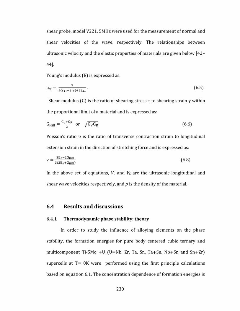
230
shear probe, model V221, 5MHz were used for the measurement of normal and
shear velocities of the wave, respectively. The relationships between
ultrasonic velocity and the elastic properties of materials are given below [42–
44].
Young’s modulus (E) is expressed as:
. (6.5)
Shear modulus (G) is the ratio of shearing stress τ to shearing strain γ within
the proportional limit of a material and is expressed as:
G
or √G G (6.6)
Poisson’s ratio υ is the ratio of transverse contraction strain to longitudinal
extension strain in the direction of stretching force and is expressed as:
v
(6.8)
In the above set of equations, VL and VS are the ultrasonic longitudinal and
shear wave velocities respectively, and ρ is the density of the material.
6.4 Results and discussions
6.4.1 Thermodynamic phase stability: theory
In order to study the influence of alloying elements on the phase
stability, the formation energies for pure body centered cubic ternary and
multicomponent Ti-5Mo +U (U=Nb, Zr, Ta, Sn, Ta+Sn, Nb+Sn and Sn+Zr)
supercells at T= 0K were performed using the first principle calculations
based on equation 6.1. The concentration dependence of formation energies is

231
summarised in Figure 6.4. It is well known that, for an alloy to be
thermodynamically stable, its formation energy ( must be negative
(exothermic) [44, 45, 46]. This indicates that the alloying elements and
combinations considered here are good β stabilisers, as they set off strong
negative offset in the ( of β-Ti-Mo alloy system. Alloying of the elements
will therefore induce a significant exothermic action on the initial composition
of the least stable β phase alloy — apart from alloy bearing Ta+Sn, whose
negative is less notable. This reflects strong chemical bonding interactions
between these atoms and the titanium–molybdenum system in the β phase,
which represents index β-phase stability in the alloy. This implies that the
ternary addition of Nb, Zr or their synergic microalloying additions are
energetically favourable to stabilising the β-phase with low composition (<5
at. %) in Ti-Mo alloy.
Based on this ab initio electronic energy calculation, the formation
energy was used to determine the index of stability and strength of the
bonding interactions of the ternary elements in Ti-5Mo system for the stability
of β-phase as Nb > Zr > Ta > Sn for an increased stability of 18.2%, 16.2%,
9.4% and 9.1% respectively. Nb, Zr, Ta and Sn microadditions could therefore
be alloyed to suppress the presence of , and phases, and a single β-
phase stabilised at low Mo concentration in Ti-Mo alloy system.
Although both Ta and Nb belong to the Im-3m (Space group number:
229), the high stability index of Nb is not unexpected as it is the nearest
neighbour element to the right of Mo in the periodic table with the closest

232
atomic size difference. The power of an atom when in a molecule to attract
electron density to itself was noted by Linus Pauling to be the element's
electronegativity. Based on this scale, Nb has 1.6 — larger than the 1.5 for Ta.
In contrast to Nb and Ta, Zr and Sn are well-known neutral elements (i.e.
completely soluble in both and β phase in the Ti-Zr or Ti-Sn binary diagram
respectively) [34]; therefore, the β stabilising effect of Zr and Sn is associated
with phase stability of the alloy, arising from the alloying elements other than
them. The decrease of 9.9% formation energy of Ti-Mo-Nb by the addition of
Zr is related simply to the rise in exothermic energy (i.e., negative formation
energy)/Ti ratio in the alloy caused by the addition of neutral elements, viz: Zr
and Sn.
Another observable feature is that, whereas Zr belongs to P63/mmc
(Space group number: 194) and has a similar HCP (hexagonal close-packed)
structure to Ti, it is next to Nb with just 2% difference in the β stabilising
effect, which is attributable to the electronegative power of 2.16 for Mo —
higher than the 1.54 of Ti — to attract electron density to itself. The influence
of the site occupation of alloying elements on the stability of β-phase was weak
and of no effect. The present results are consistent with other calculations [44,
45, 46]. Some of this trend was confirmed as experimental, as explained below.

233
6.4.2 Comparison with experimental data: Microstructure
investigation
Previously (in Chapter 5), we determined β/ (β+) phase boundary
for the composition of the least stable β phase in the Ti-Mo alloy system at Ti-
5at.% Mo (i.e. 10wt.%). Here, the least stable β-phase alloy is defined as the
alloy containing the least amount of the β-stabilising elements to get a β single
phase [2]. The composition of the least stable β-phase alloy, βc, also correlates
Figure 6.4: Formation energy (dependency on the microalloying elements for pure body centered cubic multicomponent Ti-5Mo +U (U=Nb, Zr, Ta, Sn, Ta+Sn, Nb+Sn and Sn+Zr) alloying.

234
in some ways with the emergence of many unique properties, such as non-
linear superelasticity and very low work hardening, as discussed in [34]. This
is in agreement with previous works by Blackburn et al., and by Saito et al.
[35]. In effect, we chose Ti-5 at.% Mo (Figure 6.2) as a composition to evidence
the effect of the alloying elements — namely, Mo, Nb, Ta, Zr, Hf and Sn — on β-
phase stability, microstructure evolution and Young’s modulus of β Ti-Mo base
alloys as potential biocompatible materials.
Further, ten Ti-Mo based multicomponent alloy specimens were
designed in the region across β/β+″ phase boundary [46]. The chemical
compositions, alloy designations, and β stability indicators of the
multicomponent Ti–Mo alloys are listed in Table 6.1. (In the present work, all
the compositions are given in at.% units unless otherwise noted.) The table
reveals that the chemical compositions of the multicomponent alloys are
closely related to their nominal compositions. Thus, the Ti–Mo alloys were
synthesised successfully. The phases existing in the specimen were identified
by conventional X-ray diffraction (XRD) using Ni filtered Cuk radiation.
6.4.2.1 Effects of ternary additions on Ti-Mo alloy: Phase identification
Figure 6.5 shows the XRD profile of the ternary Ti-5Mo-X(X=Nb, Ta, Zr,
Hf and Sn) alloys quenched from 1223K. All the patterns of the alloys in Figure
6.5 appear to reveal that each specimen is a single phase β. Thus, it was
apparent that Nb, Zr, Sn, Ta microadditions could suppress the presence of ,
and phases, and maintain a single β-phase at low concentration in the Ti-

235
5Mo alloy system. The present result is consistent with both the theoretical
and other previous experimental reports [12, 13, 19, 22, 23, 30], indicating
that the results are closely related. We can conclude that the plot represents
the real effect of these elements in metastable β-phase boundary of the Ti-Mo
alloy system, due probably to the large perturbation and ground state
minimisation used in the calculation.
Furthermore, the broadening of the (110) peaks of the β phase can be
seen in Ti-5Mo-Nb alloy. This can be an indication of grain refinement.
Previous studies on Ti–10Mo–10Nb reveal significant grain refinement can be
achieved by adding Nb element to Ti-Mo [19,37, 47]. Significant strengthening
Figure 6.5: XRD patterns of the ternary specimens.

236
with grain refinement can therefore be expected, in accord with the well-
known Hall–Patch relationship. On the other hand, the formation of the fine
structure also depends on the cooling rate applied during solidification. Arc
melting on a water-cooled copper hearth results in an eutectic microstructure
with grain size in the range of 200-300mm range. Copper mould casting,
however, reduces the size down to the scale of 30-70um, because a higher
cooling rate is achieved by this method. A smaller grain size corresponds to
higher yield strength. Some of the microstructural trend was confirmed
experimental, as explained below.
The trend of (110) peaks in Figure 6.5 suggests a similar trend with the
aforementioned ab initio β stability index and, apparently, the additions
effectively supressed the appearance of ω, or phases in Ti-Mo based
alloys. Similar effect on Ms, temperature was reported in Ti-30Ta-Zr [48], Ti-
15Mo-Fe [49], Ti-Cr-Zr [50], Ti-Nb-Ta [50], Ti-Nb-Zr [51]. In contrast, it was
reported that the Zr, Ta, Nb addition to Ti-Ni alloys raised the Ms temperature
[52].
6.4.2.2 Effects of ternary additions on Ti-Mo alloy: Microstructural
characteristic
The SEM micrographs of the ternary alloys are shown in Figure 6.6. It
can be observed that these alloys exhibit a pronounced microstructural
sensitivity with the alloying elements. Invariably, a significant change in

237
property can be expected, as microstructure strongly affects almost all
properties of materials [53].
Figure 6.6(a) shows the microstructure obtained after quenching Ti-
5Mo-xSn, consisting of equiaxed refined grains with average diameter ranging
from 0.1 to 10 m in size without any precipitates. It is shown in Figure 6.6(a-
d). However, many bands of obvious fibrous twinning stripes are a feature
readily observable in the entire samples in Figure 6.6. This structure will be
explained later with higher resolution micrographs of the twining structures.
The structure observed in Ti-5Mo-xNb is shown in Figure 6.6(b). The
bright batches in the micrograph show reflections of the β phase of the alloy.
While the dark patches may represent niobium-rich β, it is possible that these
are merely artifacts produced during electropolishing. Samples prepared from
a relatively hydrofluoric-sulfuric–lactic acid electrolyte also exhibited a similar
structure. Micrographs of the alloy, however, demonstrated that a single phase
could be observed; thus the results of the microstructural characterisation are
identical to those of Gordin et al. [54] and confirm the expected effect of Ti
replacement by Nb.
Figure 6.6(c) shows the microstructure of Ti-5Mo-XTa. What we can
observe in this microstructure is in good agreement with the XRD profile of the
specimen, the obvious fine needle-like structures can be ascribed to the
around the grain boundaries. In contrast to the banded structure of binary Ti-
Mo abundant in the literature [28, 29, 30], evidence of significant grain
refinement is observable in the microstructures, with average diameter

238
ranging from 50 to 200 m in size. Conversely, the microstructure obtained
for Ti-5Mo-xZr in Figure 6.6(d) has a resemblance of amorphousness. Further
investigation is required however, as Zr is an element of choice to stimulating
amorphous properties in metallic glass alloys. It was very difficult discerning
the actual grain size due to the blurry structural features of clustered lentoid
twin boundaries.
10 𝜇m
(b)
10 𝜇m
(a)

239
The role of twinning can be affected dramatically by temperature, strain
rate, texture and chemical composition [54, 55]. It is also generally understood
that {112}111 or {332}113 twinning is the most important deformation
mechanism in body centered cubic (BCC) metallic alloys [56, 57]. Recently, a
multifunctional β-titanium alloy with nominal composition of Ti-24.5Nb-
Figure 6.6: SEM microstructure in as quenched condition for (a) Ti-5M0-xSn; (b) of Ti-5M0-xNb; (c) Ti-5M0-xTa; and (d) Ti-5M0-xZr, revealing the internal structures of the studied ternary alloys.
10 𝜇m
(c)
10 𝜇m
(d)

240
100𝜇m
(a)
0.7Ta-2Zr-1.4O (at.%) exhibited multiple deformation mechanisms by
modifying the chemical composition of Gum-Metal. Despite this, the manner in
which alloying elements affect twin formation and growth has not yet been
fully elucidated; hence further comments can be made. Lagerlof [58] suggested
a mechanism that seems reasonable to interpret the formation of twins and
proposed a new model, explained elsewhere [60]. Due to lack of direct
observation of the aforementioned twinning process however, substantial
experimental evidence is still needed to prove this mechanism. We have used
stereological angle techniques on high magnified SEM to estimate and describe
twin activity and these show subtle differences in their dependence on alloying
elemental additions in Ti-Mo alloys. The SEM micrographs and chemical
composition revealing the twinning differences due to variations in ternary
element additions in Ti-5Mo alloy are presented in Figure 6.7 and Table 6.1
respectively.

241
(b)
100𝜇m
(c)
100𝜇m

242
Accordingly, straight twinnings are evident in the alloys in line with the
suggestion that non-straight mechanical twins can hardly be observed in BCC
metals [60]. Previously [60] we have seen that the included angle in BCC
crystal between [122] and [100] direction is 70.53 around the [011] axis,
which is just the crystallographic misorientation of {112}111 twins with the
matrix [61, 62]. This is equivalent to the adjacent variants of a zigzag-shaped
latte of 38-40 determined from the current view of 6.7(a)-(c). This suggests
that the zigzag-shaped lathes in Figure 6.7 (a), (b) and (c) are the {112}111β
twins with a thickness ranging between 0.1 and 1um. This indicates that the
model for zigzag–shaped [112]111 twinning is in accord with our
observation.
Figure 6.7: SEM microstructure in as quenched condition for (a) Ti-5Mo-xTa; (b) of Ti-5Mo-xZr; (c) Ti-5Mo-xSn; and (d) Ti-5M0-xNb, revealing the twinning structural differences of the ternary alloys.
(d)
10 𝜇m

243
Conversely, from the scaffolding morphology of Ti-5Mo-XNb twinnings
in Figure, 6.7(d), the observation of zigzag-shaped {112}111 twins was not
obvious. The measurements of the included angles between two adjacent twin
variants were between 60 and 65. Theoretical modelling has shown,
however, that the included angle between two adjacent twin variants of
zigzag-shaped {112}111 twins from the view of [111] matrix// [111] twin is 60
[60]. Having said this, the exert formation mechanism is not very clear. A
theoretical calculation of stacking fault energy of Ti-Nb β alloy using first
principle [62] suggested stacking energy change with increase in e/a, viz
alloying content should be one of the main factors controlling the {112}111
twins and influencing the morphology of {112}111 twins [60, 62]. In an alloy
with low stacking fault, it is difficult to restrict the extended dislocation [63].
The extended dislocation can only glide on one crystal plane, which is
implicitly why formed {112}111 twins are straight — while in alloys with
high stacking fault energy, the perfect dislocation cannot dissociate at all, and
twinning is finally suppressed.
6.4.2.3 Effects of multicomponent additions on Ti-Mo alloy: Phase
identification
Next, the changes in the constitution of alloy phases due to the synergic
addition of two elements to Ti-5Mo are presented. Figure 6.8 shows the XRD
profiles of the specimens. Aside from the alloy consisting of Ta+Sn, a
significant retention of single β-phase in the alloys in agreement with the
theory calculation and other past results [37-42] are evident. Previously [62],

244
we observed that β phase retention is reminiscent of Ti alloys with higher β
stabilising concentrations in Ti-Mo systems, therefore the β phase stability can
be ascribed to the increasing influence of β element concentrations in line with
the theoretical result.
The two major martensitic peaks at 39.0° and 39.9° correspond exactly
to those expected for 002 and 111 in the ″ phase, where a=0.301 nm, b=0.491
nm, and c=0.463 nm can be seen in the multicomponent alloy consisting of Ta
+Zr. This indicates that the synergy of Ta with Zr was not able to suppress the
appearance of the martensitic phase. Such an effect was reported for low
Zr containing β Ti type alloys, Ti-Cr-Zr [40], Ti-Nb-Sn-Zr [19]. We recall that Zr
and Sn are known neutral elements, so the β stabilising effect can be
associated with the phase stability of the alloy arising from alloying elements
other than them. In other words: when used as ternary Ti-Mo addition, the β
stabilising effect of Mo seems to have dominated, but since Ta is a mild β
stabiliser and there is wide equilibrium +β phase field and Zr and Hf has a
complete solubility in both - and β- phases in the Ti-Zr and Ti-Hf binary
diagram respectively [43], there is greater affinity for stabilising ″-phase
when alloyed with Ta element that is more or less obvious.
It is however important to mention here that no trace of ω was detected
in the ternary and quaternary alloys, implying that the effectiveness of the
elements in supressing the ω- phase is detrimental to the strength of the
alloys. We can therefore conclude that the theoretical plot represents the real

245
effect of the elements in metastable β-phase boundary of the Ti-Mo alloy
system.
6.4.3 Correlation of elastic moduli with properties for possible
biomedical applications
6.4.3.1 Elastic constants of multicomponent Ti-Mo alloy: Theory
The elastic constants and the moduli of the multicomponent Ti alloys
were evaluated by first principles total energy calculations according to eqns.
6.3, 6.4, 6.5, 6.7 and 6.8. The six important independent elastic constants —
, , , , , and — for an alloy consisting of body-centred cubic
and probable orthorhombic structures are evaluated. The evaluated values of
the elastic constants are presented in Table 6.2. In order to analyse these data,
Figure 6.8: XRD patterns of the multicomponent Ti-Mo alloys.

246
we first focus on the relative stability between the two phases. The tetragonal
shear constant, and anisotropy factor, , are also listed in Table 4.4.
⁄ is a shear parameter which corresponds to specific phonon
vibration mode in atomic structure and can be related to the stability of the
BCC structure [44] and the anisotropy factor
(A=1 for isotropy). As the
HCP-to-BCC boundaries are approached, increases, which often correlates
with deformation by twinning, and approaches zero at the β phase
boundaries. It is seen that A tends towards zero with the addition of the β
stabilising elements, which corresponds to the exothermic formation energy
obtained earlier. Accordingly, high corresponds to higher β stability as
reported earlier in the literature [64, 65, 66, 67]. A correlation was also found
between measured transition temperature (TM) and high for Ti alloys
undergoing shape memory behaviours such as TiNi based alloys [68]. This
result is in agreement with the theoretical calculation of formation energy
(Figure 6.4) at T=0K and the actual phase stability (Figures 6.6, 6.7 and 6.8) of
the multicomponent alloying in the Ti-Mo system. The polycrystalline elastic
properties such as bulk (B) and shear moduli (G) were evaluated from the
methods due to Hill [23]. Hill found that neither Voigt [21] nor Reuss [22]
relations are believed to be exact, since the Voigt equation provides an upper
limit for (G) and Reuss’s equation gives the lower limit of (G). Hill suggested
averaging by either the arithmetic or geometric mean of these two limits. The
calculated elastic moduli are shown in Table 6.3. In our previous work in
Chapter 5 and earlier [44], it was noted that most Ti alloys are textured in

247
001 direction in as cast condition. The results by [69, 19] found a variation in
Young’s modulus of Ti-Mo-Cr and Ti-Mo-Ta, Ti–(15-17) Mo–ST alloys due to
homogenisation treatments. In the present study, we evaluated the theoretical
Young’s moduli (E) of the multicomponent elastic materials expressed in the
001 direction, by eqn. 6.9:
(6.9).
denotes the young’s modulus between the 011 and 010 planes,
which is the texture direction in Ti-Mo system. Further studies are on-going in
the group to establish the exact textures and formation processes. Previously,
theoretical calculations by first principles indicated that most Ti metal alloys
have a special elastic anomaly with elastically softened directions.
In order to verify the theoretical predictions, the calculated and actual
experimental results determined that Young’s and shear moduli results of the
quenched multicomponent alloys are present for comparison in Table 6.3 and
Figure 6.9. Some important comparisons of the theoretical and experimental
elastic properties trend were confirmed, as explained below.
Materials C11 C12 C13 C33 C44 C66 A
Ti-Mo-Sn 162.23 107.26 99 65.64 39.4 28.53 27.49 1.43
Ti-Mo-Zr 155.06 97.17 98.51 95.46 36.43 32.56 28.95 1.26
Ti-Mo-Ta 153.56 104.71 99.37 106.3 36.54 -38.5 24.43 1.49
Table 6.2: Theoretical predicted elastic constants and phase stability indicators tetragonal shear modulus and anisotropy factor A for multicomponent Ti-Mo alloys are given. (For composition details, see Table 6.1.)

248
6.4.3.2 Elastic properties of multicomponent Ti-Mo alloy: Comparison of
theory and experiment
The measured dynamic elastic properties (moduli) of the quenched
multicomponent Ti-Mo alloys being studied and the theoretical determined
values are shown in Table 6.3 and Figure 6.9 as functions of the alloying
element. The elastic properties reported in the present works are the Young’s
modulus, and shear and bulk modulus represented by E, G, and B respectively.
These properties are linked directly to the tensile, shear and hydrostatic
loading respectively. As they are exclusively controlled by the interatomic
bond interactions, they can be considered the fundamental properties of any
material. Their correlation has shown specific trends with a range of
properties including hardness, yield strength and toughness [64, 70], and
where there are discrepancies these could be caused by the intrinsic effect of
different alloying elements on modulus. Very recently, a simple relationship
Ti-Mo-Nb 174.89 116.35 95.9 111.6 34.39 33.83 29.27 1.17
Ti-Mo-Ta-Sn 160.85 104.4 91.84 125.45 37.57 27.75 28.43 1.32
Ti-Mo-Nb-Zr 163.99 108.28 89.25 98.1 34.7 31.52 55.71 0.63
Ti-Mo-Ta-Zr 152.3 122.45 90.99 125.45 35.67 -30.3 14.93 2.39
Ti-Mo-Zr-Sn 161.63 120.64 91.41 90.03 35.52 24.78 20.50 1.73
Ti-Mo-Nb-Sn 172.55 121.23 90.1 100.1 36.5 25.47 25.66 1.42
Ti-Mo-Ta-Nb 173.62 141.24 96.14 148.9 28.44 32.75 16.19 1.76
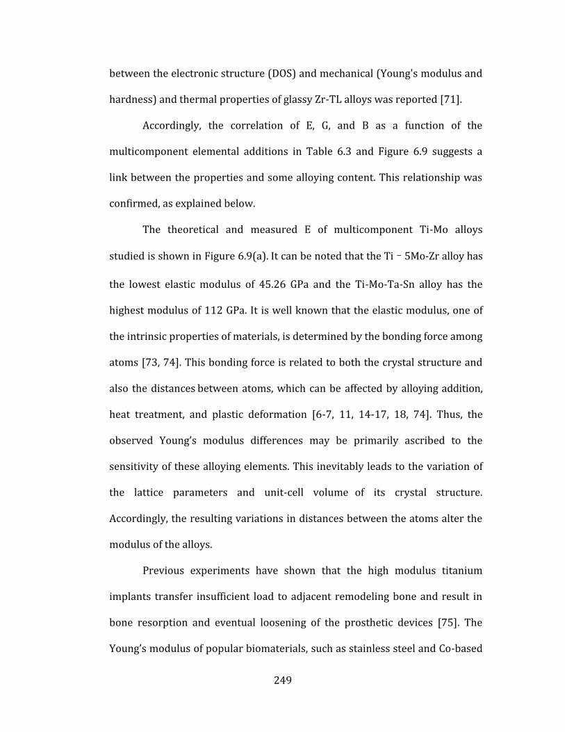
249
between the electronic structure (DOS) and mechanical (Young's modulus and
hardness) and thermal properties of glassy Zr-TL alloys was reported [71].
Accordingly, the correlation of E, G, and B as a function of the
multicomponent elemental additions in Table 6.3 and Figure 6.9 suggests a
link between the properties and some alloying content. This relationship was
confirmed, as explained below.
The theoretical and measured E of multicomponent Ti-Mo alloys
studied is shown in Figure 6.9(a). It can be noted that the Ti–5Mo-Zr alloy has
the lowest elastic modulus of 45.26 GPa and the Ti-Mo-Ta-Sn alloy has the
highest modulus of 112 GPa. It is well known that the elastic modulus, one of
the intrinsic properties of materials, is determined by the bonding force among
atoms [73, 74]. This bonding force is related to both the crystal structure and
also the distances between atoms, which can be affected by alloying addition,
heat treatment, and plastic deformation [6-7, 11, 14-17, 18, 74]. Thus, the
observed Young’s modulus differences may be primarily ascribed to the
sensitivity of these alloying elements. This inevitably leads to the variation of
the lattice parameters and unit-cell volume of its crystal structure.
Accordingly, the resulting variations in distances between the atoms alter the
modulus of the alloys.
Previous experiments have shown that the high modulus titanium
implants transfer insufficient load to adjacent remodeling bone and result in
bone resorption and eventual loosening of the prosthetic devices [75]. The
Young’s modulus of popular biomaterials, such as stainless steel and Co-based

250
alloys, is 206 and 240 GPa respectively, which is significantly higher than that
of bone tissue (∼10–40 GPa). The elastic modulus of cp-Ti, near β and β Ti
alloys also varies between 121 and 57 GPa, which is higher than 42.19 and 45
.26 GPa obtained from theory and experiment on our newly designed Ti-5Mo-
Zr alloy, which is much closer to natural bone that will minimise the bone
resorption arising from the stress shielding effect and consequently increase
the long-term stability of the implants. The values from theoretical and
measured results confirm a good agreement of the Young’s modulus with ± 5%
and increase in the sequence Zr < Ta+Zr < Zr+Sn < Nb+Sn < Ta < Sn < Nb < Ta <
Ta+Nb < Ta+Sn < Nb+Zr < Ta+Sn. This sequence is slightly different from the
sequence of β phase stability in Figure 6.4.
There are different reports on Young’s moduli of the various phases in
Ti alloys. It was reported that the -phase exhibits a much higher elastic
modulus as compared with the β-phase and the elastic modulus of the phases
of titanium alloys increase in the sequence β <″ < < [9, 26]. Ho et al. [11]
found, however, that the martensite ″ phase with 7.5% Mo has the lowest
modulus among ″ and β phases in the Ti–Mo system, whereas Hao et al. [26]
reported that the ″ andβ phases have nearly the same Young’s modulus in the
Ti–29Nb–l3Ta–4.6Zr alloy. Moreover, Kim et al. [76] reported that the
metastable β phase has lower elastic modulus than stable β phase. Kim’s and
Hao’s reports are consistent with the present study and in good agreement
with other theoretical [44, 45, 46] and experimental [11, 13, 14, 19] results.
First, we recall that the XRD profile of Ta+Zr, which possesses the second

251
lowest Young’s modulus and contains the two major martensitic peaks at 39.0°
and 39.9°, corresponds exactly to those expected for (002) and (111) in the ″
phase with a=0.301 nm, b=0.491 nm, and c=0.463 nm, thus indicating that the
synergy of Ta with Zr was not able to suppress the appearance of the
martensitic phase. Such an effect was reported earlier for low Zr containing
metastable β Ti type alloys, Ti-Cr-Zr [40], Ti-Nb-Sn-Zr [19]; thus the result is
due to the intrinsic effect of alloying elements [12].
In Chapter 4 we observed from EBSD analysis that most binary Ti-Mo
alloys are textured in 001 direction in as cast condition. Additionally, the
reports by [69, 19] found a large variation in Young’s modulus of Ti-Mo-Cr and
Ti-Mo-Ta, Ti–(15-17) Mo alloys respectively, due to homogenisation
treatments. Consequently, the Young’s modulus (E) of the multicomponent
alloys was expressed in the 001 direction, by eqn. 6.9. The excellent
relationship obtained between theory and experimental data is notable.
Although the exert basis for the coincidence requires more studies, there are
ample reasons to infer that other factors are involved; and if it were a
coincidence, what could possibly explain the effect of the observed 001
texture in as cast Ti–Mo alloy systems.
It is evident that the shear modulus G trend in Figure 6.9(c) could not
reflect similar agreement as in E. It is not surprising since each manifests
different characteristics of materials: E is a measure of resistance to a change
in atomic separation distance within the plane of the bond, and so can be
determined from the linear portion of the interatomic potential. G quantifies

252
the resistance to shear loading. Elastic moduli are therefore controlled by
interatomic interactions and so may be considered a fundamental property,
whereas G is proportional to the activation energy for a shear event in
materials. Based on this premise, it is suggested [77] that experimentally
measured moduli (by resonant ultrasound spectroscopy and ultrasonic time-
of-flight measurements) may not be controlling macroscopic deformation
since they are an average across the whole sample. B (Figure 6.9(b)), since it
corresponds to a volumetric dilatation, is dependent on the electronic
properties of a solid, i.e. the compressibility of the electron gas.
To verify the influence of texture on the predicted Young’s modulus,
DFT-GGA calculation was performed for Ti-5Mo-xZr alloy (i.e. the lowest
Young’s modulus alloy) and found 64.12 GPa and 20.23 for and
respectively. This is presumably why most Ti alloys was predicted to be
elastically anisotropic [41]. As Table 6.2 and Figure 6.9(a) reveal, however, this
material is actually quite isotropic. In general the theoretical predictions for
the Young’s modulus are within a difference of 5% with experimental values.
The small discrepancy could reflect differences in temperature, minor
experimental error or approximations inherent to DFT-GGA.

253

254
Figure 6.9: Plots revealing the effect of alloying elements on the Young’s (E), Bulk (B)and Shear moduli, (G) of the multicomponent Ti-Mo alloys.

255
Materials
Ti-Mo-Sn [present study] 76.85 79.05 24.41 101.4 -0.25 0.37 39.4
28.8
TMZF (Ti–12Mo–6Zr–2Fe) [41 ] 79.5
Ti–12Mo–5Zr [78](sol) 64.5
Ti–12Mo–5Zr [78](Hom) 90
Ti-Mo-Zr [present study] 42.19 45.26 33.47 93.7 0.21 0.41 36.4 25.9
Ti-Mo-Ta [present study] 68.66 81.51 20.41 68.4 -0.61 0.37 36.5 31.5
Ti–6.6Mo–1.47Ta [54] 74
Ti-Mo-Nb [present study] 81.93 96.37 44.21 80.6 0.61 0.30 34.4 37.0
Ti–6.6Mo–1.47Nb [ 13,54] 105
Ti-Mo-Ta-Sn [present study] 88.67 112.66
28.94 74.9 0.46 0.25 37.6 45.1
Ti-Mo-Nb-Zr [present study] 97.87 108.14
34.33 76.9 0.22 0.27 34.7 42.7
Ti-Mo-Ta-Zr [present study] 53.15 60.10 8.04 45.1 -0.39 0.33 35.7 23.5
Ti-Mo-Ta-Nb [present study] 86.91 106 11.58 82.7 -0.67 0.29 28.4 41.4
Ti-Mo-Zr-Sn [present study] 58.51 14.42 -0.37 35.5
Ti-Mo-Nb-Sn [present study] 72.50 23.84 -0.60 36.5
c.p. Ti (grade 2)[79] 105
ASTM F75 (Co–Cr–Mo)[15] 220
V316 (stainless steel)[15] 379
Ti–6Al–4V (grade 5) [79] 114
Table 6.3: Comparison of theoretical predicted and measured elastic parameters are given, along with literature data for other BCC 1Ti alloys of the multicomponent Ti-Mo alloys in units of GPA. (For composition details, see Table 6.1.)

256
6.5 Summary and concluding remark
The major findings of Chapter 6 are summarised as follows.
Based on the DFT-GGA electronic calculation implemented on CASTEP
code for stable solid solutions, a number of metastable body-centred cubic
ternary and multicomponent alloys were experimentally and theoretically
designed to correspond to the composition formula of Ti-5Mo +U (U=Nb, Zr,
Ta, Sn, Ta+Sn, Nb+Sn and Sn+Zr) supercells at T=0K. Using the first principle
calculations, their β phase thermodynamic stability, microstructure and
mechanical properties — especially low Young’s modulus — were obtained,
which compared well with experimental validation of properties. The main
findings of this chapter are as follows:
The trend of the electronic formation energy attests to significant
sensitivity of the system to micro-elemental addition. The calculated
parameters qualitatively track the known elemental behaviour in Ti-Mo binary
system, which indicates that DFT-GGA is favourable to the computational
screening of relative phase stability of alloys.
On an atom-for-atom basis, the β phase stability trend shows an
increasing potency in the sequence Nb > Zr > Ta > Sn with ternary micro-
additions and Nb+Zr > Ta+Nb > Ta+Sn > Ta+Zr > Ta+Hf for the complex alloys
respectively. In agreement with theoretical results, both the experimental
analyses show single β phase, indicating the micro additions are enough to
suppress the presence of and ″ in the ternary and other complex alloys.

257
The calculated and measured Young’s modulus of the investigated alloy
varies between 45.19 and 118GPa. Our newly designed Ti-Mo-Zr alloy
exhibited the lowest Young’s modulus of 45 GPa (42.19GPa from theory),
which is significantly lower than elastic modulus of conventional metallic
implant materials (cp-Ti, near β and β Ti alloys) — which varies between 121
and 57 GPa — and much closer to natural bone, which will minimise the bone
resorption arising from the stress shielding effect and consequently increase
the long-term stability of the implants.
Both theory and experiment confirm a good agreement of the Young’s
modulus within ± 5% and increase in the sequence Zr < Ta+Zr < Zr+Sn <
Nb+Sn < Ta < Sn < Nb < Ta < Ta+Nb < Ta+Sn < Nb+Zr < Ta+Sn in Ti-Mo system.
This sequence is slightly different to the sequence of β phase stability, implying
that the effectiveness of low Young’s modulus strategy might not be explicitly
dependent on β phase microstructure stability. Thus, the strategy can be a
good step towards developing future metallic biomaterial with bone matching
Young’s modulus for orthopaedic implant applications.
Finally, this work suggests a link between cast material texture and the
directionality of calculated Young’s modulus of the alloys. Although more
study is obviously needed to establish this, the calculated Young’s modulus in
the direction showed a good agreement with cast Young’s modulus
values.

258
6.6 References
[1] KESSLER: “Titanium-the Space-age Metal", ASTM Standardization News (1984) 26-27. (1b) H.D Nishimura T: J. Power Energy Syst. 2 (2008), 530–537. [1c] Weiss I and Semiatin S.L: Mater. Sci. Eng. A243 (1998) 46–65. [2] Aziz-Kerrzo M., Conroy K. G., Fenelon A. M., Farrell S. T.; Breslin CB: Biomaterials 22(2001), 531. [3] Yu S. Y., Scully J. R.; Corrosion 53 (1996), 965. [4] Godley R., Starosvetsky D., Gotman I.; J. Mater Sci –Mater Med. 17 (2006), 63. [5] Li S. J., Yang R., Li S., Hao Y. L., Cui Y. Y., Niinomi M.; Wear 257(2004), 869. [6] Niinomi M.; “Recent metallic materials for biomedical applications”, Metall. Mater Trans. A 33 (2002), 477–86. [7] Niinomi M.; “Mechanical properties of biomedical titanium alloys”, Mater Sci. Eng. A 243 (1998), 231–6. [8] Long M., Rack H. J.; “Titanium alloys in total joint replacement—a materials science perspective”, Biomaterials 19 (1998), 1621–39. [9] Hon Y. H., Wang J. Y., Pan Y. N.; “Composition/phase structure and properties of titanium–niobium alloys”. Mater Trans 44 (2003), 2384–90. [10] Matsumoto H., Watanabe S., Hanada S.; “Microstructures and mechanical properties of metastable β TiNbSn alloys cold rolled and heat treated”, J. Alloy Compd. 439 ;( 2007), 146–55. [11] Ho W. F., Ju C. P., Chern Lin J. H.; “Structure and properties of cast binary Ti–Mo alloys”, Biomaterials 20 ;( 1999), 2115–22.
[12] Delvat E., Gordin D. M., Gloriant T., Duval J. L., Nagel M. D.; “Microstructure,
mechanical properties and cytocompatibility of stable beta Ti–Mo–Ta sintered
alloys”, J. Mech Behav Biomed Mater 1;(2008),345–51.
[13] Gordin D. M., Gloriant T., Texier G., Thibon I., Ansel D., Duval J. L.;
“Development of a β-type Ti–12Mo–5Ta alloy for biomedical applications
cytocompatibility and metallurgical aspects”, J. Mater Sci. Mater M 15;
(2004),885–91.

259
[14] Zhou Y. L., Niinomi M., Akahori T.; “Effects of Ta content on Young's modulus and tensile properties of binary Ti–Ta alloys for biomedical applications”. Mater- Sci. Eng. A 371, (2004), 283–90. [15] Zhou Y. L., Niinomi M., Akahori T.; “Decomposition of martensite α″ during aging treatments and resulting mechanical properties of Ti–Ta alloys”, Mater- Sci. Eng. A 384; (2004), 92–101. [16] Zhou Y. L., Niinomi M.; “Microstructures and mechanical properties of Ti-50 mass% Ta alloy for biomedical applications”, J. Alloys Compd. 466; (2008), 535–42. [17] Zhou Y. L., Niinomi M.; “Ti–25Ta alloy with the best mechanical compatibility in Ti–Ta alloys for biomedical applications”, Mater-Sci Eng. C 29 (2009), 1061–5. [18] Ferrandini P. L., Cardoso F. F., Souza S. A., Afonso C. R., and Caram R.; “Aging response of the Ti–35Nb–7Zr–5Ta and Ti–35Nb–7Ta alloys”. J Alloys Compd. 433(2007), 207–10. [19] Hanada S., Matsumoto H., Watanabe S.; “Mechanical compatibility of titanium implants in hard tissues”, International Congress Series; (2005), 239–47. [20] Silva H. M., Schneider S. G., Neto C. M.; “Study of nontoxic aluminium and vanadium-free titanium alloys for biomedical applications”, Mater Sci. Eng. C 24;(2004), 679–82.
[21] The University of Sheffield and Web Elements Ltd., UK, website.
http://www.webelements.com/niobium/physics.html
http://www.webelements.com/tantalum/physics.html
http://www.webelements.com/molybdenum/physics.html.
[22] He G., Eckert J., Dai Q. L., Sui M. L., Löser W., Hagiwara M. et al.; “Nanostructured Ti-based multi-component alloys with potential for biomedical applications”. Biomaterials 24; (2003), 5115–20. [23] Bagariatskii I. A., Nosova G. I., Tagunova T. V.; “Factors in the formation of metastable phases in titanium-base alloys”. Sov Phys Dokl. 3; (1959), 1014–8
[transl. of Dokl. Akad. Nauk. SSSR, Vol.122; (1958), 593–596.
260
[24] Fedotov S. G., Chelidez T. V., Kovneristyy Y. K., Sanadze V. V.; “Phase transformation during heating of metastable alloys of the Ti–Ta system”, Phys. Met. Metall. 62; 2 (1986), 109–13. [25] Niinomi M.; “Multifunctional low-rigidity β-type Ti-Nb-Ta-Zr system alloys as biomaterials”, Biomaterials 24; (2003), 2675-84.
[26] Hao Y. L., Li S. J., Sun S. Y., Zheng C. Y., Yang R.; “Elastic deformation behaviour of Ti–24Nb–4Zr–7.9Sn for biomedical applications”, Acta Biomater 3(2007), 277-286.
[27] Matsumoto H., Watanabe S., Hanada S.; “Beta TiNbSn Alloys with Low Young's Modulus and High Strength”, Mater Trans. 46 ;(2005), 1070-84. [28] Wang K.; “The use of titanium for medical applications in the USA”, Mater-Sci. Eng. A, 213 (1996), 134–7.
[29] Ho W. F.; “A comparison of tensile properties and corrosion behaviour of cast Ti–7.5Mo with c.p. Ti, Ti–15Mo and Ti–6Al–4V alloys”, J Alloy Compd. 464; (2008), 580–3. [30] Ying-Long Z. and Dong-Mei L.; “Microstructures and mechanical properties of Ti–Mo alloys cold-rolled and heat treated”, Mater-Charact. 62; (2011), 931-937. [31] “Least square Unit cell refinement” Program after Appleman and Evans (1973), implementation by R.G. [32] Segall M. D., Philip J. D. L., Probert M. J., Pickard C. J., Hasnip P. J., Clark S. J. and Payne M. C.; “First-principles simulation: ideas, illustrations and the CASTEP code”, J. Phys. Condens. Mater 14 (2002), 2717–2744. [33] W. Kohn and Sham L.: “Self-consistent equation’s including exchange and correlations affects”, Phys. Rev. A 140 (1965), 1133. [34] Perdew J. P., Burke K. and Ernzerhof M.; “Generalized Gradient Approximation Made Simple”, Phys. Rev. Letts. 77, (1996), 3865. [35] Duthie J. C., Pettifor D. G.; Phys. Rev. Lett. 38 (1977), 564. [36] Mandi S., Ruschenbach B.; Surf.Coat. Technol. 156 (2002) 276-283. [37] Gasser B., in: D.M Brunette, P. Tengvall, M. Texfor, P. Thompson (Eds.). Titanium in Medicine, Springer, New York (2001) 673-701.

261
[38] Okazaki Y., Ito Y, Tateishi T: MATER. Trans. JIM 37(1996) 843-849. [39] Pharr, G. M., Oliver, W. C.; “Measurement of thin film mechanical properties using nanoindentation”, MRS Bulletin 17, (1992), 28–33. [40] Volinsky A. A., Gerberich W. W.; Microelectron. Eng.69 (2003) 519-527. [41] Majumdar P., Singh S. B. and Chakraborty M.; “Elastic modulus of biomedical titanium alloys by nano-indentation and ultrasonic technique-A comparative study”, Mater. Sci. Eng. A 489(2008) 419-425. [42] Augereau F., Laux D., Allais L., Mottt M. and Caes C.; Ultrasonics 46(2007), 34- 41. [43] Dogbmane M., Hadjoub F., Dogbmane A. and Hadjoub Z.; Mater. Lett. 61(2007) 813-816. [44] Raabe D., Sander B., Fri´ak M., Ma D., Neugebauer J.; “Theory-guided bottom-up Design of Beta-titanium alloys as bioMaterials based on first principles calculations: Theory and experiments”, Acta Materialia 55, (2007), 4475–4487. [45] Dai J. H., Wu X., Song Y. and Yang R.; “Electronic structure mechanism of martensitic phase transformation in binary titanium alloys”, J. App. Phys.112 (2012), 123718-24 [46] Abdel-Hady M., Hinoshita K., Morinaga M.; “General approach to phase stabililty and elastic properties of b-type Ti-alloys using electronic parameters”, Scripta Mater. 55, (2010)477-480. [47] Tadaki T., Tokoro M. and Shimizu K.; Mater. Trans. JIM. 16; (1975) 285. [48] Louzguina-Luzgina L. V., Dmitri V. L. and Inoue A.; “Influences of additional alloying elements (V, Ni, Cu, Sn, B) on structure and mechanical properties of high-strength hypereutectic Ti–Fe–Co bulk alloys”, Intermetallics 14 (2006) 255–259. [49] Xu l. J., Chen Y. Y., Liu X. G. and Kong F. T.; “The microstructure and properties of Ti–Mo–Nb alloys for biomedical application,” J. Alloys and Compd. 453 (2008) 320–324. [50] Ikeda. M. et al.; J. Alloy. Mater. Trans.45, (2004), 1106. [51] Mina X. H., Emura S., Sekido S., Nishimura T., Tsuchiya K. and Tsuzaki K.; “Effects of Fe addition on tensile deformation mode and crevice corrosion resistance in Ti–15Mo alloy”; Mater. Sci. & Eng. A 527 (2010) 2693–2701.

262
[52] Tang X., Ahmed T., and Rack H. J.; J. Mater.Sci.35 (2000) 1805. [53] Otsuka, K. and Ren X.: Intermetallics 7(1999), 511. [54] Gordin D. M., Gloriant T., Nemtoi Gh, Chelariu R., Aelenei N., Guillou A. and
Ansel D.; Mater. Lett. 59 (2005) 2959–2964.
[55] Meyers M. A., Vohringer O. and Lubranda V. A.; Acta Mater 49, (2001) 4025. [56] Ikeda M., Komatsu S., Sigmoto T. and Kamei K. J.: Jpn. Inst.Met.53, (1989) 664. [57] Blackburn M. J. and Feeney J. A.; J. Inst. Met. 99 (1971) 132. [58] Lagerlof K. P. D.; Act Metall. 41 (1993) 2143. [59] Yang Y., Li G. P., Cheng G. M., Li Y. L., Li Y. F., Yang K., and Ge P.; Acta Mater. 58, (2010) 2778. [60] Yang Y., Li G. P., Wang H., Wu. S. Q., Zhang L. C., Li Y. l. and Yang K.; “Formation of zigzag shaped {112}111 β mechanical twins in Ti-24.5Nb-0.7Ta-2Zr-1.4O alloy”, Scr. Mater. 66 (2012) 211-214. [61] Hsiung L. M. and Lassila D. H.; Scripta Mater.38 (1998) 1371. [62] Yu N. Y., Yang P., Qiang W. J. and Chen L.; Foundation Materials Science and Technology press, 1990. [63] Davis R., Flower H. M. and West D. R. F.; “Martensitic transformations in Ti-Mo alloys”, J. Mater. Sci. 14 (1979) 22–28. [64] Fisher E. S. and Dever D.; “Relation of the c′ elastic modulus to stability of
b.c.c. transition metals”, Acta Met. 18(1970), 265-269.
[65] Saito T., Furuta T., Hwang J., Kuramoto S., Nishino K., Suzuki N., Chen R., Yamada A., Ito K., Seno Y., Nonaka T., Ikehata K., Nagasako N., Iwamoto C., Ikuhara Y., and T. Sakuma; Science 300, (2003), 464. [66] Ikehata H., Nagasako N., Furuta T., Fukumoto A., Miwa K., and T. Saito; Phys. Rev. B 70, (2004), 174113. [67] Li T., Morris J. W., Jr., Nagasako N., Kuramoto S., and Chrzan D. C.; Phys.
Rev. Lett. 98, (2007) 105503.

263
[68] Hu Q. M., Yang R., Lu J. M., Wang L., Johansson B. and Vitos L.; Physic.Rev.B
76, (2007), 224201.
[69] Xingfeng Zhao, Niinomi M., Nakai M., Hieda J.; “Beta type Ti–Mo alloys with changeable Young’s modulus for spinal fixation applications”, Acta Biomater. 8 (2012) 1990-1997. [70] Gu X. J., Mcdermott A. G., Poon S. I. and Shiflet G. J.; Appl. Phys. Let.88, (2006) 211905. [71] Lewandowski J. J., Wang W. H., and Greer A. L.; Phil.Mag.Lett.85 (2005) 77-87. [72] Ristić R., Stubičar M., and Babić E.; Philos. Mag. 87 (2007) 5629–5637 and reference therein. [73] Ikeda M., Komatsu S. Y., Sowa. I., and Niinomi M.; Met. Mater. Trans. A 33
(2002) 487–493.
[74] Geetha M., Mudalki M. U., Gogia A. K., Asokamani R., and Raj B.; Corros. Sci.
46, (2004) 877–892.
[75] Hao Y. L., Niinomi M., Kuroda D., Fukunaga F., Zhou Y. L., Yang R. and
Suzuki A.; Met. Mater. Trans. A 33 (2002) 3137–3144.
[76] Kim H. S., Kim W. Y. and Lim S. H.; Scripta Mater. 54 (2006) 887–891.
[77] Plummer J. D: PhD Thesis “On the physical aspects that control mechanical
deformation in bulk metallic glasses”, Department of Materials Science and
Engineering University of Sheffield (2012).
[78] Changli Z., Zhang X. and Cao P.; “Mechanical and electrochemical
characterization of Ti–12Mo–5Zr alloy for biomedical application”, J.Alloys and Compd. 509, (2011) 8235– 8238. [79] Bertrand E., Gloriant T., Gordin D., Vasilescu E., Drob P., Vasilescu and C., Drob S. I.; J. Mech. Behav. Biomed. 3 (2010) 559–564.

264
Chapter 7 Defining Material Properties by Elastic Constant
Systematics
7.1 Introduction
Elastic constants of materials and alloys are of interest because of the
information they provide concerning the nature of the binding forces in solids.
Elastic constants of some simple BCC metals have been extensively
investigated, theoretically and experimentally, in a wide range of compositions
and temperatures [1]. The relationship between the elastic properties and the
importance of as an index of BCC-lattice stability is usually considered from
the microscopic point of view of electronic structure (as characterised by the
electron per atom ratio or e/a parameter).
Of interest here is a unified analysis of alloys transformable by stress-
induced formation (SIM) via elastic constant systematics obtained by first
principle calculations. Several type alloys, such as Ti-Mo, that possess
transforming (SIM) properties undergo a first order transformation above a
certain composition range (in the case of -type Ti alloy), revealing a
martensitic transformation from (disordered BCC) to an orthorhombic
martensite phase. They are called SIM alloys because they are inherently
metastable in nature and prone to transformation if additional energy, such as
stress or hydrostatic pressure, is provided. They are, in some cases, reversible

265
from phase in the absence of the additional energy, which is the basis
for the continued search for the shape memory effect in -type Ti alloy.
Although the shape memory effect has been reported in Ti-Mo alloy [2-
5], Ti-Nb alloy [6-8] and Ti-V alloy [9], fundamental understanding is still
insufficient in Ti-based shape memory alloy. The explanation in terms of the
elastic moduli has not being significantly extended beyond the commonly
encountered stability criteria.
Previously, in Chapters 4 and 6, we investigated the elastic constant of
binary and multicomponent Ti-Mo alloys and interpreted the changes in
moduli from the T-matrix solution of the elastic constants. The present section,
as an extension, will systemise the specific case of the transformable (stressed
induced martensitic) BCC Ti alloys in the context of continuum elastic theory
uniquely determined by the three elastic constants — , and —
derived from theoretical and experimental data. In a cubic crystal,
corresponds physically to shear resistance on a (100) plane, to
shear resistance on a (110) plane, and to the bulk modulus B
representing resistance to volume change ⁄ caused by hydrostatic
pressure P: ⁄ = ⁄ . In addition, the shapes of the three characteristic
acoustic surfaces of a cubic symmetry crystal depend only on the ratios of
these elastic constants for satisfying the thermodynamic constraints —
, | | and [10].
To do this, we rely heavily on a Blackman diagram [11]. In 1938,
Blackman introduced this diagram — which is a dimensionless plot of reduced

266
elastic stiffness coefficient ⁄ versus ⁄ — to search for material
with a high Debye temperature, which led to the surprising result that
materials with similar chemical bondings fall into the same region of the
diagram, despite large differences in their absolute stiffness coefficients.
Recently, by incorporating important bonding conditions in its
representations, the parameter has been used to provide illuminating
descriptions of generalities of elastic behaviour in metallic glass [12].
We note that experimental and computation details pertaining to this
aspect of the present work are given in Chapters 4, 5 and 6.
7.2 Results and discussions
Figure 7.1 shows a Blackman’s diagram of BCC metals and alloys
containing a range of calculated and experimental elastic property data from
the literature in Table 7.1. The data represent a wide-range of BCC metallic
alloys in terms of composition and behaviour. Lines (blue dash lines) radiating
from the upper-left corner represent lines of constant Zener shear–
deformation elastic anisotropy, ⁄ , and the 45 dashed line
denote . They also correspond to the important central interatomic
forces relationship in cubic SIM behaviours displayed a cluster over and into a
small region (at lower 0.4 and 0.5) of the diagram, in very
close proximity to the central interatomic forces line (Pc>0) and A0.5. This
may indicate a similarity in interatomic bonding type (not strength). Other
non-SIM alloys are also found at a well-defined area over the large
267
and low region bounded by A 0-1 3. The other BCC metals cluster
over larger but still well defined areas. We attribute the larger areas to
differences in interatomic bonding within the same crystal structure. The
Blackman diagram is therefore very useful for the present study on
interatomic bonding in BCC metals and alloys.
First, we note the physical meaning of the cluster as an indication of
near-same interatomic bonding, despite large differences in composition and
size. A previous criterion [13] provides an insight into the close link between
crystal structure and mechanical properties of solids, ascribing strong metallic
non-directional bond-bending forces to materials with a positive value of
Cauchy pressure (Pc>0), while the negative value is indicative of strong
convalency, directional interatomic bond angularity and strong resistance to
bond bending.

268
The position of the SIM alloy signifies its positive Cauchy pressure,
suggesting a non-directionality bonding framework, while its close proximity
to the Cauchy line is indicative of the inherently instability and inability to
withstand high shear stress. Born and Huang [14] pointed out that the Cauchy
relationship is unfavourable for lattice stability, and that lattices interacting
with particularly large central forces tend to be unstable. Both and
correspond physically to shear resistances and to phonons
on a (100) plane in cubic a crystal. This may suggest the both low shear moduli
( and ) are implicit characteristic of the lattice instability
Figure 7.1: Blackman diagram displaying the congregation of some BCC alloys with respect to the interatomic bonding forces. Also indicated are elastic anisotropy (blue dash lines), ⁄ and the Cauchy pressure line, . The identities of the elements/alloys are given in Table 7.1.

269
exhibited by SIM alloys, leading to cooperative atomic movement during
deformation. It has been suggested that that the physical origin is the smaller
principal strains (< 3%) involved in transformation, rather than those
required to produce the HCP structure [1], coupled with identical specific
volume of and phase.
It is also important to point out that we found a good degree of
correlation between the calculated data of Ti-(10-23) Mo and the experimental
SIM data. We do, however, attribute the presence of the lean alloy composition
(Ti-(3-6) Mo) — i.e. alloys 1 and 2 — in the negative Cauchy region (Pc<0) to
the imaginary cubic nature assigned during calculation to alloys of
predominantly orthorhombic martensitic phase. For this symmetry,
immediate difficulties arise because the three cubic independent elastic –
stiffness coefficients lose their important physical meaning.
Figure 7.2 shows a Blackman diagram FCC metals and alloys, to which
the Cauchy condition and elastic anisotropy lines are also indicated. We found
that FCC SIM alloys fall near the Cauchy line in small clusters similar to the BCC
ones in Figure 7.2. It terms of the vs placement, the two
groups are bound differently in the Blackman diagram. FCC alloy are bound by
large and moderate . The high elastic anisotropy as observed in
the FCC SIM alloys, however, led Zener to predict successfully low-
temperature martensitic transformation in Li and Na to an FCC crystal [15].
This may suggest a similar conclusion. The non SIM alloys and the other FCC
metals fall rather far apart into a well-defined relatively small area. This

270
therefore suggests strongly different interatomic bonding, probably caused by
their different electron configurations.
Given the findings, it is important to plot both BCC and FCC SIM alloys
together on the same Blackman diagram. Most materials fall into (Pc>0)
however, and materials in the region Pc<0 are known to be exceptionally rare
— with the exception of Barium (BCC metal, 9), which may be described as a
free element never found in nature because of its high chemical reactivity due
Figure 7.2: Blackman diagram showing a congregation of some FCC alloys with respect to the interatomic bonding forces. Also indicated are elastic anisotropy (blue dash lines), ⁄ and the Cauchy pressure line, . The identities of the elements/alloys are given in Table 7.1.

271
to its non-central interatomic force. Nguyen-Manh and colleagues concluded
that negative Cauchy pressure in many –body repulsive terms can arise from
an overlap of the free electron like sp-band electrons when compressed by the
d-electrons in BCC [16]. Apart from -plutonium (BCC metal: 11), an s1
electron material is known as the most anisotropic FCC element and all
departures are towards the region.
By comparing the elastic properties of these phases in Figure 7.3 and
Table 7.1, several trends become evident: first, the location of both FCC and
BCC SIM alloys in the Blackman diagram. These are bound within the same
axial distance of similar Poisson’s ratio. In a Blackman diagram, the poisons
ratio averages over all crystallographic directions. Pugh [17] established a
relationship between Poisson ratio and ductility, while Koster-Franz [18]
described its connection with interatomic bonding. As seen in Figure 7.3, their
common indicators are similar to Poisons ratio regime (0.3 0.324) and share
a close proximity to the Cauchy pressure. The physical significance of this is
that materials with similar Poison’s ratios behave very similarly mechanically.
Thus, a low poisons ratio primarily results in shape change and provides
strong support for the high ductility and psuedoelasticity exhibited by SIM
alloys.
7.3 Conclusions
We attest in this study that the Blackman diagram can be used as an
effective tool to theoretically analyse predictions and experimental deductions
of some basic important behaviours of alloys. We have demonstrated a SIM

272
relation between the central interatomic forces and poisons ratio, and high
ductility of SIM alloys.
.
Figure 7.3: Blackman plot combining some BCC and FCC metals and alloys in one diagram, revealing the relationships between the two SIM alloys groups. The identities of the elements/alloys are given in Table 7.1.

273
7.4 References
[1] Fisher E. S., Westlake D. G., and Ockers S. T.; Phys. Status Solidi A 28
(1975)59 1-602
[2] Grosdidier T., and Philippe M. J.; Mater. Sci. Eng. A 291 (2000) 218-223.
[3] Ho F. W, JU. C. P., and Chern Lin J. H.; Biomaterials 24(199) 2115-2122.
[4] Hosoda H., Ohmatsu Y., and Miyazaki S.; Trans. MRS-J(26) (2001) 235-237.
[5] Hosoda H., Hosoda S., and Miyazaki S.; Trans. MRS-J(26) (2001) 243-246.
[6] Baker C.; Mater. Sci. J 5(1871) 92-100.
[7] Nitta K., Watanabe S., Masakashi N., Hosoda H., and Hosoda S.; Structural
Biomaterials for the 21st century (TMS, 2001)25-34.
[8] Hosoda H., Fukui Y., Imamura T., Wakeshima S., Miyazaki S., and Inoue I.;
Mater. Sci. Forum 426-432 (2003)3121-3123.
[9] Duerig T., Albrecht J., Richter D., and Fischer D.; Act. Metal. 30(1982) 2161-
2172.
[10] Nye, J. F.; Physical Properties of Crystals (Oxford University Press,
London, 1957), 32.
[11] Blackman M.; Proc. Roy. Soc. London 164, (1938) 62.
[12] Plummer J. D., and Todd I.; Applied Phys. Lett. 98(2011) 021907
[13] Pettifor; Mater.Sci& Tech. 8(1992), 345.
[14] Born M., and Huang H.; Dynamic Theory of crystal lattices (Oxford
University Press, London, 1954), 152.
[15] Zener C.; Elasticity and Anaelasticity of Metals (University of Chicago
Press, Chicago, 1948) 16.
[16] Soderlind P.; Adv.Phys. 47(1998), 959.
[17] Pugh S.; Philos. Mag. 45(1954), 823.
[18] Koster W., and Franz H.; Metall. Rev.6(1961)1.
[19] Ren X. et al.; Mag. 79(1999) 31-41.
[20] Hatcher N., Kontsevo Yu O., and Freeman A. J.; Phys.Rev.B 80(2009) 1-18.
[21] Li S. J., Cui T. C., Hao Y. L., and Yang R.; Acta Biomat 4 (2008) 305-17.

274
[22] Nobuhito S., Niinomi M., and Akahori T.; Mater. Trans. 45, No. 4 (2004)
1113–1119.
[23] Zhengjie L., Wan L., Xiaobing X., Weijie L., Qina J., and Zhang D.; Mater. Sci.
and Eng. C 33 (2013) 4551–4561.
[24] Hou F. Q., Li S. J., Hao Y. L., and Yang R.; Scripta Mater. 63 (2010) 54–57.
[25] Tane M., Nakano T., Kuramoto S., Hara M., Niinomi M., Takesue N., Yano T.,
and Nakajima H.; Acta Mater. 59 (2011) 6975–6988.
[26] Kim H. Y., Ikehara Y., Kim. J. I., Hosoda H., and Miyaaki S.; Acta Metall.54
(2006) 2419.
[27] Talling R. J., Dashwood R. J., Jackson M., Kuramoto S., Dye D.; Scr. Mater. 59
(2008) 669.
[28] Hao Y., Li S., Sun B., Sui M., and Yang R.; Physical Rev. Letts. 98 (2008), 1-4.
[29] Paszkiewicz and Wolski; J. Phys. (Conference series) 104 (2008), 012038.
[30] Mañosa L et al.; Phys. Rev. B 49 (1994), 9969-9972.
[31] Zhou L., Cornely P., and Trivisonno J:Ultrasonic symposium (1990)1389-
1329.
[32] Sedlak P., Seiner H., Landa M., Novak V., Sittner P., and Manosa Li; Acta
Materialia 53 (2005) 3643–3661.

275
This work C11 C12 C12/C11 C44/C11 Ref.
1 Ti-3Mo 159.3 115 0.72 1.21 2 Ti-6Mo 111.3 69.07 0.62 0.93 3 Ti-10Mo 167 19.6 0.12 0.081 4 Ti-14Mo 179.2 17.9 0.10 0.074 5 Ti-18Mo 192.6 16.3 0.085 0.066 6 Ti-23Mo 197.5 16 0.081 0.051
Non-SIM (BCC)alloys
1 Ti50Ni30Cu20 209 183 0.88 0.17 [19]
2 Ti-50Ni 165 140 0.85 0.21 [20]
3 Ti-29Nb-13Ta-4.6Zr 67.1 39.9 0.87 0.19 [21]
4 Ti-30Nb-10Ta-5Zr 128 92 0.86 0.24 [22]
5 Ti-35Nb 163.5 142 0.87 0.22 [23]
6 Ti-30Nb-5Ta-5Zr 70 30 0.87 0.185 [24]
7 Ti-32.7Nb-11.6Ta-4.49Zr-0.066O-0.052N 137 91.1 0.86 0.12 [25]
Non SIM (FCC) alloys
1 Ag-75Au 230 161.5 0.702 0.33 [19]
2 Cu-4.17Si 117 85.2 0.73 0.64 [19]
3 α-Ag-2.4Zn 190 162 0.85 0.43 [19]
4 α-Cu-9.98Al 199 179 0.89 0.50 [19]
5 α-Cu-22.7Zn 158.9 136.2 0.86 0.43 [19]
SIM(BCC) alloys
1 Ti-35.37Nb 130.2 52 0.40 0.078 [26]
2 Ti-35Nb-2Zr-0.7Ta 183 31.4 0.17 0.15 [25
3 Ti-35.4Nb-1.9Ta-2.8Zr-0.37O 122 27 0.22 0.11 [25]
4 Ti-24.1Nb-4Zr-8.06Sn-0.15O 140 26.3 0.19 0.16 [25]
5 Ti-35Nb-10Ta-4.6Zr-0.16O 102.5 36 0.16 0.12 [27]
6 Ti-23.9Nb-3.75Zr-8.01Sn-0.04O 157.2 36 0.26 0.127 [27]
7 Ti-24Nb-4Zr-7.9Sn-0.17O
0.23 0.22 [27]
8 Ti-24Nb-4Zr-7.6Sn-0.07O 122 31.4 0.26 0.21 [25]
9 Ti-35.2Nb-10.5Ta-4.97Zr-0.091O-0.014N 140 27 0.19 0.1 [27]
10 Ti-23.9Nb-3.8Zr-7.61Sn-0.08O 102.5 26.3 0.12 0.13 [27]
11 Ti-24Nb-4Zr-7.9Sn 157.2 46 0.29 0.27 [28]
SIM(FCC) alloys
1 Cu44.9- 50Zn 125 80 0.64 0.6 [19]
2 Au47.5-50Cd 142 96.77 0.68 0.53 [19]
3 Ag45-50Zn 132.8 83.16 0.63 0.57 [19]
4 -FeNi 209 183 0.65 0.54 [29]
5 CuAlNi 142.8 93.7 0.66 0.59 [30]
Table7.1: Elastic constant of some BCC and FCC metals and alloys.

276
BCC elements C12/C11 C44/C114 Ref.
1 V 0.52 0.19 [29]
2 Nb 0.59 0.13 [29]
3 Ta 0.60 0.31 [29]
4 Mo 0.38 0.28 [29]
5 W 0.5 0.43 [29]
6 Li 0.83 0.78 [29]
7 Na 0.82 0.75 [29]
8 K 0.79 0.73 [29]
9 Ba 0.43 0.7 [29]
FCC elements
[29]
2 Au 0.83 0.22 [29]
3 Pd 0.79 0.3 [29]
4 Pt 0.74 0.2 [29]
5 Ag 0.76 0.39 [29]
6 Cu 0.76 0.43 [29]
7 -Co 0.69 0.6 [29]
8 α-Sr 0.65 0.39 [29]
9 -Fe 0.68 0.5 [29]
10 Ni 0.62 0.51 [29]
11 δ-Pu 0.78 0.96 [29]
6 B2-NiTi 162 104 0.64 0.52 [31]
7 Cu2.726A11.122Ni 0.152 137 89.2 0.65 0.59 [32]
8 Cu2.742Al1.105Ni0.152 136 81.763 0.65 0.61 [32]

277
Chapter 8
Conclusions and Further work
8.1 Conclusions
The results gathered from experiments described in this thesis suggest
that the modelling solution approach (as carried out in the present work) can
be used effectively to predict and study important properties of metallic alloys.
Furthermore, it has been shown that first principle calculations (DFT) as
implemented in the CASTEP code are a very effective technique in
characterising the phase stability, formation energy, elastic properties and
deformation behaviour of superelastic materials. The good agreement
between the theoretical calculations and experimental verified data for
thermodynamic stability, composition and elastic constant justifies the use of
the approach for evaluating property in the present work.
In order to understand the intrinsic mechanism by which alloying
elements influence thermodynamic phase stability, we compared the total
electronic density of states (DOS) of ″ and β crystal structures. From this
viewpoint, it is thought that the structural stability change in the Ti-Mo system
is connected to the lowering of N(EF) due to hybridisation of the d- electronic
states of the Mo atom. This provides for the increasing covalency in the
bonding of the two atoms.

278
The structural properties relating to the orthorhombic phase
transformation in Ti-Mo alloy system has been studied using optical
microscope, SEM, EBSD and Rietveld refinement of XRD profiles. The
formation of the orthorhombic phase has been ascribed to three main reasons:
(a) in view of the eightfold coordination around each (Ti, Mo) atom with four
additional neighbours at a slight greater distance. The formation of the α in
preference to α in Ti-Mo binary alloy beyond a certain Mo critical
concentration could be a reflection of a tendency for Mo to retain the eightfold
coordination obtained in BCC titanium; (b) atomic size difference can also lead
to distortion of the crystal structure; and (c) assuming the major influence of
atom size is ignored, the movement/shift of the atoms along y -atomic
coordinate without breaking the group symmetry is another possible
explanation. Additionally, the orthorhombicity in this alloy decreases as Mo
content increases.
The trend of the Young’s moduli of the samples followed a similar
direction to the hardness, suggesting that might be responsible for the low
hardness and Young’s modulus, since both are structurally related properties.
It is worth noting, however, that the Young’s modulus of the Ti-6Mo was even
lower than that of the Ti-6-4 alloy. This advantage of ″ orthorhombic
structure can be exploited to further reduce the Young’s modulus of future
metallic biomaterials.
Based on the DFT-GGA electronic calculation, a number of metastable
body centered cubic ternary and multicomponent alloys were experimentally

279
and theoretically designed to correspond to the composition formula of Ti-
5Mo +U (U=Nb, Zr, Ta, Sn, Ta+Sn, Nb+Sn and Sn+Zr) supercells at T= 0K. The
trend in the electronic formation energy attests to the significant sensitivity of
the binary Ti-Mo alloy system to phase stability and elastic moduli with micro-
elemental addition, which indicates that DFT-GGA is favourable to the
computational screening of relative phase stability and other p of alloys. Our
newly designed Ti-Mo-Zr alloy exhibited the lowest Young’s modulus, with 45
GPa (42.19GPa from theory), which is significantly lower and much closer to
natural bone than the elastic modulus of conventional metallic implant
materials (cp-Ti, near β and β Ti alloys), which vary between 121 and 57 GPa.
We have suggested by analysis of data in this study that the Blackman
diagram can be used effectively to theoretically analyse predictions and make
experimental deductions about the behaviours of alloys and by this have
demonstrated a link between the central interatomic forces (Cauchy pressure)
and the Poissons ratio with superelastic of SIM alloys.
8.2 Further works
Although the results of the present work suggest a link between cast
material texture and the directionality of calculated Young’s modulus of the
alloys, further work is needed to obtain a more detailed understanding of the
operative texture mechanisms. In particular, the significance of the role of the
initial microstructure (1) on the elastic modulus, and (2) in inhibiting the
emergence of textures requires investigation. Further higher resolution TEM

280
work is recommended to establish the effect of texture on the elastic property
of the alloys.
Furthermore, the results of this work have shown that the mechanical
properties of binary Ti-Mo alloy systems are very sensitive to chemical
composition. There is consequently a good scope to improve the alloys for
specific applications. For example, the amount of transformation strain could
be optimised through control of chemical composition or through control of
specimen texture. A systematic approach is required to analyse the effect of
alloying elements on the interplay between twinning, SIM and slip during
subsequent loading.
It is envisaged that, with further theoretical research, SIM alloy can be
designed using the elastic constant systematics from DFT. First principle
calculations may be able to portray the shape memory effect of
multicomponent Ti-Mo alloys akin to other Ni-Ti and Ti-Nb based alloys. This
would broaden the portfolio of applications of these alloys even further,
offering a more in-depth understanding of what physical and microstructural
factors enable a material to exhibit the shape memory effect. This would
suggest that further work is needed to redefine the composition window and
other factors considered before alloys can be designed on first principles.